Deep S³PR: Simultaneous Source Separation and Phase Retrieval Using Deep Generative Models (Long Version)

Abstract

This paper introduces and solves the simultaneous source separation and phase retrieval (S³PR) problem. S³PR is an important but largely unsolved problem in a number application domains, including microscopy, wireless communication, and imaging through scattering media, where one has multiple independent coherent sources whose phase is difficult to measure. In general, S³PR is highly under-determined, non-convex, and difficult to solve. In this work, we demonstrate that by restricting the solutions to lie in the range of a deep generative model, we can constrain the search space sufficiently to solve S³PR.

Code associated with this work is available at https://github.com/computational-imaging/DeepS3PR.

Abstract

This supplement provides a detailed description of how simultaneous source separation and phase retrieval (S³PR) appears and limits performance in a real-world computational optics application; seeing through scattering media. It also provides additional experimental results tested at a lower signal-to-noise ratio (SNR).

1 Introduction

We define the S³PR problem as follows. Recover the signals $x_{1},~{}x_{2},~{}\ldots,~{}x_{L}\in\mathcal{C}$, where $\mathcal{C}$ is some subset of $\mathbb{R}^{n}$ (e.g. the set of natural images), from a noisy measurement vector $y\in\mathbb{R}^{m}$ given by

$$y=\sum_{l=1}^{L}|\mathbf{A}_{l}x_{l}|^{2}+w,$$ (1)

where the square is elementwise, the measurement matrices $\mathbf{A}_{l}\in\mathbb{C}^{m\times n}$ are known for all $l$, and $w$ represents additive noise. In the remainder, we focus on the special case $\mathbf{A}_{1}=\mathbf{A}_{2}=\ldots=\mathbf{A}_{L}$.

For $L=1$ this problem is just standard phase retrieval (PR), a problem for which myriad solutions exist [1, 2, 3, 4]. However, when $L>1$ things become significantly more challenging. In particular, one is forced to disentangle the components of $y$ that came from $x_{i}$ from the components that came from $x_{j}$, with $i\neq j$. That is one must solve a source separation (SS) problem as well as multiple PR problems.

Motivation

S³PR is intrinsic to a variety of different application domains where one measures the intensity of a field formed by multiple independent coherent sources. Under these conditions, the fields within a single source add but the intensities between distinct sources add. This situation appears in partially coherent phase imaging microscopy [5, 6], correlation-based imaging through thin scattering media and around corners with highly separated or multi-spectral objects [7, 8, 9, 10, 11], transmission-matrix based imaging through thick scattering media with multiple independent sources [12, 13], and even multiple source localization with mmWave 5G [14]. A detailed description of S³PR’s role in correlation-based imaging through scattering media is provided in the supplement.

Despite the prevalence of the S³PR problem, no general solution to to S³PR yet exist. The lack of existing solutions is likely because S³PR is simply too non-convex and under-determined to be solved with conventional algorithms. While a cascaded solution, that is SS followed by PR, could work in principle, Section 5 demonstrates that in practice the components $|\mathbf{A}x_{1}|^{2},~{}|\mathbf{A}x_{2}|^{2},~{}\ldots,~{}|\mathbf{A}x_{L}|^{2}$ are too similar to reliably separate with traditional SS algorithms.

Our contribution

In this work we solve the S³PR problem by imposing strong but realistic priors on the reconstructed signals. In particular, we constrain $x_{1},~{}x_{2},~{}\ldots,~{}x_{L}$ to lie in the range of a generative neural network $G:\mathbb{R}^{k}\rightarrow\mathbb{R}^{n}$ with $k\ll n$. That is, $\mathcal{C}=\text{Range}(G)$ and for all $x_{l}\in\mathcal{C}$ there exists some latent vector $z_{l}\in\mathbb{R}^{k}$ such that $x_{l}=G(z_{l})$.

Using this constraint, we recover $x_{1},~{}x_{2},~{}\ldots,~{}x_{L}$, with our estimates $\hat{x}_{l}=G(\hat{z}_{l})$, from $y$ by solving the optimization problem

$$\hat{z}_{1},\hat{z}_{2},\ldots,\hat{z}_{L}=\operatorname*{arg\,min}_{z_{1},z_{2},\ldots,z_{L}}{\big{\|}}y-\sum_{l=1}^{L}|\mathbf{A}G(z_{l})|^{2}{\big{\|}}^{2}_{2},$$ (2)

using an alternating descent algorithm.

To our knowledge, this work represents the first general solution to S³PR. Accordingly, it opens up a variety of application domains. In Section 5 we apply this method to simulated Gaussian, coded-diffraction-pattern (CDP), and Fourier measurements and demonstrate the successful recovery of numbers ($\mathcal{C}=$ MNIST dataset) and articles of clothing ($\mathcal{C}=$ Fashion MNIST dataset [15]).

Limitations

Our results have a few limitations. First, our present reconstructions are low resolution and come from fairly restrictive classes — digits and articles of clothing. Second, while we provide extensive evidence that deep generative models can be used to solve S³PR, our current results are purely empirical. S³PR remains a highly under-determined and non-convex problem and deriving the conditions under which it can and cannot be solved remains an important but open problem.

2 Related work

While the S³PR problem is new, both PR and SS have been studied extensively and have a vast literature. Likewise, while not previously used for S³PR, deep generative models have recently been applied to a range of inverse problems. We now highlight a few of the most prominent of these works.

2.1 Phase retrieval

The optics community has studied the PR problem continuously since the 1970s [1, 2, 3, 4, 16, 17]. In the last decade, PR has caught the attention of the optimization and machine learning community as well [18, 19, 20, 21]. For a benchmark study of over a dozen popular PR algorithms, see PhasePack [22]. No existing PR algorithm can handle S³PR — they are designed for a fundamentally different forward model that does not mix measurements.

Compressive phase retrieval

[23] recognized that if one imposed a prior on the reconstruction one could perform PR using significantly fewer measurements. This initial work has been followed up by numerous others that have imposed more and more elaborate priors on the reconstruction [24, 25, 26, 27]. Again, none of these algorithms can handle S³PR.

Multi-source phase retrieval

A handful of works [28, 29, 30, 31] have studied multi-source PR, defined as recovering $x_{1},~{}x_{2},~{}...,~{}x_{L}$ from

$$y=|\sum_{l=1}^{L}\mathbf{A}_{l}x_{l}|^{2}.$$

This model resembles Equation (1), but note that here the mixing occurs before the non-linearity. This difference makes the reconstruction problem significantly easier as it enables the application of a standard PR algorithm to recover $\sum_{l=1}^{L}\mathbf{A}_{l}x_{l}$ followed by a standard SS algorithm to recover $x_{1},~{}...,~{}x_{L}$. In contrast, the S³PR problem defined by Equation (1) does not lend itself to similar cascaded solutions as existing SS algorithms struggle to separate $|\mathbf{A}x_{1}|^{2}$ and $|\mathbf{A}x_{2}|^{2}$ when $x_{1}$ and $x_{2}$ are drawn from the same distribution/class; see the reconstructions in Section 5.

Phase retrieval and blind demodulation

In various imaging applications, one records measurements of a signal $x_{1}$ that is illuminated by an unknown signal $x_{2}$. In this context, the measurement model becomes

$$y=|\mathbf{A}(x_{1}\circ x_{2})|^{2},$$

where $\circ$ denotes the Hadamard (elementwise) product. While solutions to this problem exist [32, 33], the fact that mixing occurs before the non-linearity makes the problem fundamentally different from S³PR.

Partially coherent phase retrieval and source recovery

When one images a fixed object $x$ with multiple unknown Fourier plane (Köhler) illumination sources, one is presented with a constrained S³PR problem

$$y=\sum_{l=1}^{L}|\mathbf{A}(x_{l})|^{2}\text{ with }x_{l}=x\circ\mathbf{F}e_{l},$$

where $e_{1}$, $e_{2}$, … $e_{L}$ are unknown 1-hot vectors representing the location of an illumination source and $\mathbf{F}$ is a 2-D discrete Fourier transform matrix which models their propagation to the object plane. By capturing multiple measurements of this form at different stand-offs (which corresponds to selecting a particular measurement matrix $\mathbf{A}$) one can reframe this problem as deconvolution and solve it using conventional algorithms [5, 6].

2.2 Source separation

Traditional SS algorithms assume that the sources to be separated are statistically independent and that there are as many or more observations as there are unknowns [34, 35, 36]. When this is not the case, the problem is known as under-determined SS and is much more challenging.

Under-determined SS, which features prominently in reflection removal and hyperspectral imaging, has been accomplished by imposing priors on the reconstructed signals, for instance that they are sparse [37, 38, 39, 40, 41] or group sparse [42] in some basis or have other structural properties that can be exploited [43]. Under-determined SS can also be accomplished with convolutional neural networks [44, 45, 46].

2.3 Inverse problems with deep generative models

Deep generative models have been used to solve a variety of under-determined inverse problems.

Compressive sensing

The idea of solving the compressive sensing problem by recovering the latent vectors of a deep generative model was first proposed in [47]. This work has been followed up by a number of papers which have sought to improve the speed [48, 49, 50, 51, 52] and generalizability [53, 54, 55] of the method.

Phase retrieval

PR with generative models was introduced in [56] and [57]. This method has since been accelerated in [58] and applied to various PR problems in [59, 60].

We note in passing that optimizing the latent variables of untrained networks, following ideas proposed in [61], can also be used to impose priors in order to help solve the PR problem [62, 63].

Other inverse problems

For the sake of completeness, we note that optimizing the latent variables of a deep generative models has also been used to perform blind demodulation [64], blind deconvolution [65], matrix decomposition [66], and source separation [67]. We also note that optimizing the latent variables of untrained neural networks has been used for a variety of image decomposition tasks, including source separation [68].

3 Naive S³PR solutions

Here we describe two naive solution with which one might approach S³PR. As we will demonstrate in Section 5, the first approach is largely ineffective. The second does not generalize.

3.1 SS followed by PR

Given measurements

$$y=\sum_{l=1}^{L}|\mathbf{A}x_{l}|^{2}+w,$$

one could first use an under-determined SS algorithm to estimate $|\mathbf{A}x_{1}|^{2},~{}|\mathbf{A}x_{2}|^{2},~{}\ldots,~{}|\mathbf{A}x_{L}|^{2}$ and then use a PR algorithm ($L$ times) to recover $x_{1},~{}x_{2},~{}\ldots,~{}x_{L}$ from these estimates. That is, one could solve potentially solve S³PR by performing under-determined SS followed by PR.

The aforementioned SS step requires one to separate measurements $|\mathbf{A}x_{1}|^{2},~{}|\mathbf{A}x_{2}|^{2},~{}\ldots,~{}|\mathbf{A}x_{L}|^{2}$ from their sum. Representative measurements and their sum are presented in Figure 1. Separating such signals is a highly under-determined SS problem for which standard SS algorithms, like non-negative matrix factorization, do not apply. Instead, one needs to use prior information, e.g. sparsity in some basis/dictionary, about the measurements to unmix them.

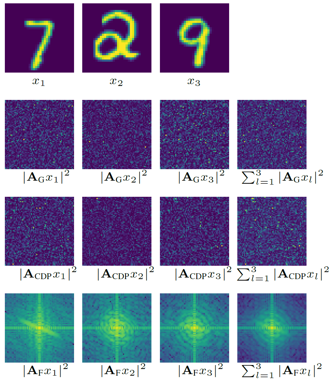
Figure 1: Visualization of measurements. Examples of signals and their measurements with Gaussian ($\mathbf{A}_{\text{G}})$, CDP ($\mathbf{A}_{\text{CDP}}$), and Fourier ($\mathbf{A}_{\text{F}}$) measurement matrices. The Fourier measurements are displayed in log scale and the Gaussian and CDP measurements were reshaped from $64^{2}\times 1$ vectors into $64\times 64$ images for visualization. The various measurements have little obvious structure and separating each of them from their sum is a challenging problem.

As a best attempt at dictionary-based under-determined SS, for each dataset and measurement matrix pair we learn a unique 500 element dictionary, $\mathbf{D}$ (for a total of 6 dictionaries). Each dictionary was formed using the K-SVD algorithm [69] and was optimized to form one-hot representations of $60\,000$ training measurements, which were specific to the dataset and the measurement matrix.

With a dictionary in hand, we then perform SS by finding an $L$-hot representation of $y$ in this dictionary using orthogonal matching pursuit (OMP) [70]. That is, we use OMP to approximately solve

$$\|y-\mathbf{D}\alpha\|_{2}^{2}\text{ subject to }\|\alpha\|_{0}=L,$$ (3)

where $\|\alpha\|_{0}$ is the cardinality of $\alpha$. The result allows us to form the estimates

$$\widehat{|\mathbf{A}x_{l}|^{2}}=D_{l}\alpha_{l},$$ (4)

where $\alpha_{l}$ is the $l^{th}$ non-zero element of $\alpha$ and $D_{l}$ is the column of $\mathbf{D}$ (i.e., the element of the dictionary) associated with $\alpha_{l}$.

Following SS, we reconstruct $x_{1},~{}x_{2},~{}\ldots,~{}x_{L}$ by solving $L$ phase retrieval problems by applying gradient descent to the loss

$$\hat{x}_{l}=\operatorname*{arg\,min}_{x}\|\widehat{|\mathbf{A}x_{l}|^{2}}-|\mathbf{A}x|^{2}\|^{2}_{2}.$$ (5)

We also experimented with the widely used Gerchberg–Saxton algorithm [1] but found that it ran far slower and offered worse performance.

As we will demonstrate in Section 5, this approach is largely ineffective at solving S³PR.

3.2 Discriminative neural networks

One could potentially use discriminative deep neural networks to perform the source separation step within the above algorithm. One could even use a discriminative neural network to directly learn a mapping from mixed measurements, $y$, to images, $x_{1},~{}x_{2},\ldots,x_{L}$. However, with either approach such a network would become specific to the forward model, the number of signals in the mixture, the distribution of the signals in the mixture, and potentially the signal-to-noise ratio (SNR) – obtaining the results in our paper would have required training 36 separate networks.

In contrast, our proposed method generalizes across forward models, SNRs, and the number of signals in the mixture – we trained only two networks.

4 S³PR using deep generative models

A better way to perform S³PR is to leverage deep generative models as priors.

Recovering latent variables

We recover images $x_{1},~{}x_{2},~{}\ldots,~{}x_{L}$, with our estimates $\hat{x}_{l}=G(\hat{z}_{l})$, from $y$ by solving the optimization problem

$$\hat{z}_{1},\hat{z}_{2},\ldots,\hat{z}_{L}=\operatorname*{arg\,min}_{z_{1},z_{2},\ldots,z_{L}}{\big{\|}}y-\sum_{l=1}^{L}|\mathbf{A}G(z_{l})|^{2}{\big{\|}}^{2}_{2},$$ (6)

using an alternating descent algorithm. That is, we iteratively compute the loss (6) and take a gradient step (with momentum) with respect to $z_{1}$, then compute the loss and take a gradient step (with momentum) with respect to $z_{2}$, etc. In practice, we found alternating descent (using the ADAM optimizer [71]) provided a near monotonic reduction of the loss and ran in two minutes on an Nvidia Titan RTX GPU.

For time/resource-sensitive applications, one could also use an alternating projection algorithm [49, 58] or more advanced methods like AMP [48, 51] or ADMM [52], which can provide significantly faster convergence.

Generative model

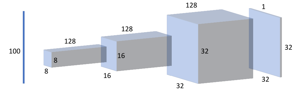
Figure 2: Simplified DC-GAN network architecture. A simple convolutional neural network, which maps a 100 dimensional latent vector to a $32\times 32$ image, serves as our generative model.

Following [47] we use a variation of the DC-GAN [72] architecture as our deep generative model, $G(z)$. Our generator network is illustrated in Figure 2. It takes a 100 dimensional latent vector, $z\in\mathbb{R}^{100}$, as an input and applies a fully connected layer followed by a reshaping operation and batch normalization to form an $8\times 8\times 128$ dimensional feature map. This feature map is then upsampled $2\times$, convolved with $128$ different $3\times 3$ filters, batch normalized, and feed through a leaky ReLU to form a $16\times 16\times 128$ feature map. This feature map is then upsampled, convolved with $64$ different $3\times 3$ filters, batch normalized, and feed through another leaky ReLU to form a $32\times 32\times 64$ feature map. Finally, this feature map is convolved with a single $3\times 3$ filter and passed through a tanh nonlinearity to form the generated image.

We train one such DC-GAN network to produce MNIST digits and another to produce Fashion MNIST articles of clothing. Each network was based off the Pytorch implementation of DC-GAN from [73] and was trained using the code’s default parameters. The networks were trained using the training portion of their respective datasets and tested, as described in the next section, on a subset of the testing portion.

5 Experimental results

We now apply the two proposed methods to Gaussian, coded diffraction pattern (CDP), and Fourier measurements of images of numbers and articles of clothing. We denote the under-determined SS followed by PR approach described in Section 3.1 with “USS + PR”. We call the deep generative model based approach from Section 4 “Deep S³PR”.

Measurement settings

In each of our tests, the images have a resolution of $32\times 32$ ($n=1024$) and we use $4\times$ oversampling ($m=4096$, $\mathbf{A}\in\mathbb{C}^{4096\times 1024}$). For the case of Fourier measurements, we achieve the oversampling by first zero padding the $32\times 32$ images to $64\times 64$. We apply the algorithms to mixtures of two, three, and four images. We add white Gaussian noise to all our measurements, such that they have an SNR of $50$. Lower SNR results are included in the supplement.

We apply the algorithms to Gaussian, CDP, and Fourier measurements to generate Figures 1, 2, and 3, respectively. To generate each of the quantitative results presented in Tables 1, 2, and 3 we apply the algorithms to 10 sets of images and compute the average normalized mean squared error (NMSE). To account for the labeling ambiguity, that is the solution $\hat{x}_{1}=A$, $\hat{x}_{2}=B$ is equivalent to the solution $\hat{x}_{1}=B$, $\hat{x}_{2}=A$, we report the loss associated with the ordering of the solutions that produces the minimum error. There is a sign ambiguity, that is $\hat{x}_{1}=A$ is an equivalent solution to $\hat{x}_{1}=-A$, that we similarly account for. Likewise, for Fourier measurements, we account for the flip ambiguities of the solutions by searching, over all flips left-right and up-down, for the one that minimizes the error.

Algorithm settings

Both the sequential USS + PR algorithm and Deep S³PR method are implemented in Pytorch. Their respective optimization problems are solved with the ADAM optimizer with a learning rate of $0.02$. ADAM’s momentum decay terms $b_{1}$ and $b_{2}$ are set to their default values of $0.9$ and $0.999$ respectively. For USS + PR, we minimize the under-determined SS loss (3) by running the ADAM optimizer for $2\,000$ iterations. The PR loss (5) is similarly minimized by running the ADAM optimizer for $2\,000$ iterations. For Deep S³PR we minimize the loss (6) by running the ADAM optimizer for $2\,000$ iterations. For both USS + PR and Deep S³PR we perform 5 restarts. For USS + PR, at each restart the estimates $\alpha$ and $x_{1},~{}x_{2},~{}\ldots,~{}x_{L}$ are initialized with random i.i.d. Gaussian vectors with mean zero and unit variance. Similarly, for Deep S³PR at each restart the latent vectors $z_{1},~{}z_{2},~{}\ldots,~{}z_{L}$ are initialized with random i.i.d. Gaussian vectors with mean zero and unit variance. For both, we use the result with the smallest residual error, $\|y-\sum_{l}|\mathbf{A}\hat{x}_{l}|\|^{2}$, as our final solution.

5.1 Gaussian measurements

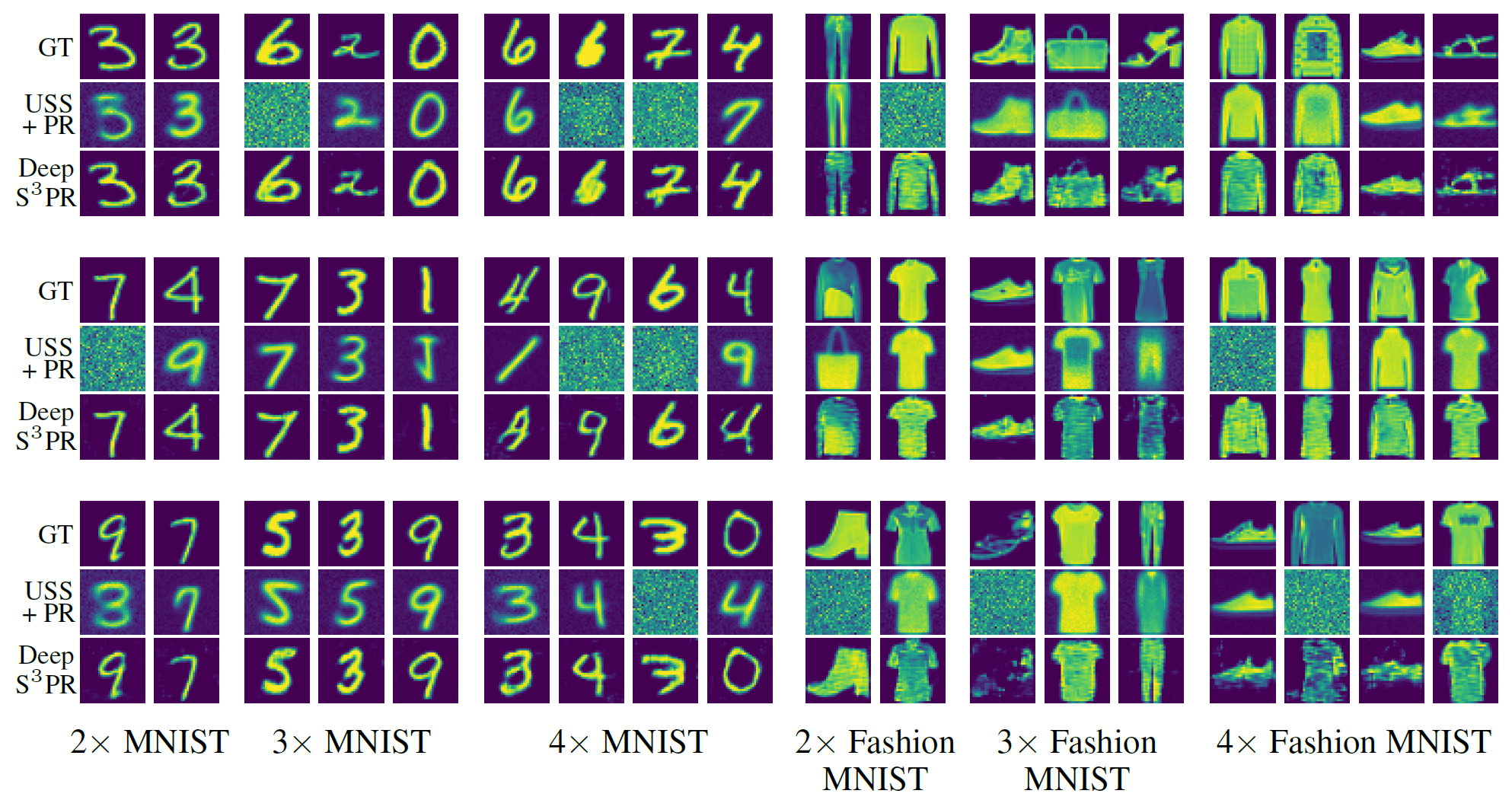
Figure 3: Reconstructions from mixtures of two, three, or four images with a Gaussian measurement matrix. With Gaussian measurements, the sequential algorithm (middle row of each set) can often recovery an image or two from the mixture, it almost always makes a few mistakes. In contrast, the proposed Deep S³PR technique (bottom row of each set) largely succeeds in recovering up to four mixed images. Ground truth shown in the top row of each set.

Table 1: Average NMSE across 10 sets of test images with Gaussian measurement matrices.

	2$\times$ MNIST	3$\times$ MNIST	4$\times$ MNIST	2$\times$ Fashion MNIST	3$\times$ Fashion MNIST	4$\times$ Fashion MNIST
USS + PR	$.54\pm.56$	$.52\pm.51$	$.43\pm.32$	$.55\pm.37$	$.40\pm.23$	$.49\pm.14$
Deep S3PR	$.02\pm.02$	$.02\pm.02$	$.04\pm.04$	$.08\pm.03$	$.13\pm.09$	$0.14\pm.07$

We first test the proposed S³PR methods on complex-valued Gaussian measurement matrices. The elements of our measurement matrices are drawn from an i.i.d. circular Gaussian distribution (the real and imaginary parts of each element are drawn from i.i.d. distributions).

Results

Figure 1 demonstrates that Deep S³PR is very effective with Gaussian measurement matrices. Even with mixtures of four images, Deep S³PR produces near perfect reconstructions of MNIST digits and recognizable, though imperfect, reconstructions of Fashion MNIST articles of clothing as well. In contrast, the sequential solution to S³PR produces significant errors with even just two images. The quantitative results, presented in Table 1, mirror these findings.

5.2 Coded diffraction pattern measurements

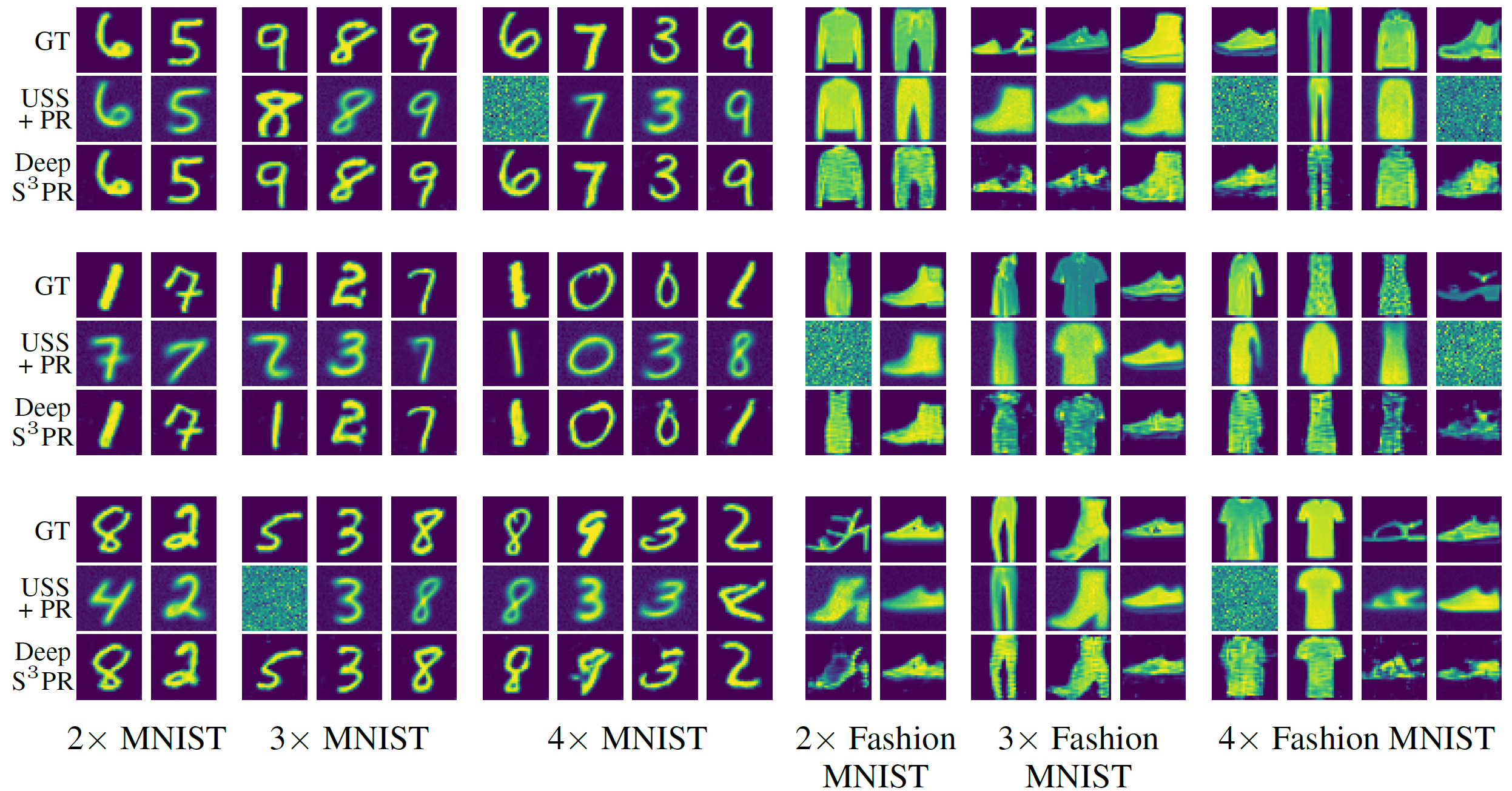
Figure 4: Reconstructions from mixtures of two, three, or four images with a CDP measurement matrix. With CDP measurements the sequential algorithm (middle row of each set) often produces errors with just two images. In contrast the proposed Deep S³PR method (bottom row of each set) again succeeds in recovering up to four mixed images. Ground truth shown in the top row of each set.

Table 2: Average NMSE across 10 sets of test images with CDP measurement matrices.

	2$\times$ MNIST	3$\times$ MNIST	4$\times$ MNIST	2$\times$ Fashion MNIST	3$\times$ Fashion MNIST	4$\times$ Fashion MNIST
USS + PR	$.40\pm.34$	$.33\pm.18$	$.44\pm.15$	$.30\pm.31$	$.60\pm.45$	$.52\pm.29$
Deep S3PR	$.01\pm.01$	$.03\pm.03$	$.05\pm.03$	$.05\pm.03$	$.12\pm.09$	$.10\pm.04$

We next test our methods on simulated CDP measurements, which were first proposed in [74]. The CDP measurement matrix can be written as

$$\mathbf{A}=\left[\begin{array}[]{ll}\mathbf{F}\mathbf{D}_{1}\\ \mathbf{F}\mathbf{D}_{2}\\ \mathbf{F}\mathbf{D_{3}}\\ \mathbf{F}\mathbf{D}_{4}\end{array}\right],$$ (11)

where $\mathbf{F}$ represents the two dimensional Fourier transform and $\mathbf{D}_{1},~{}\mathbf{D}_{2},~{}\mathbf{D}_{3},$ and $\mathbf{D}_{4}$ are diagonal matrices whose diagonal entries are drawn uniformly from the unit circle in the complex plane.

Results

Figure 2 and Table  2 demonstrate that Deep S³PR is largely effective with CDP measurement matrices as well. Meanwhile, as it did with Gaussian measurements, the sequential solution to S³PR makes errors starting with just two images.

5.3 Fourier measurements

Figure 5: Reconstructions from mixtures of two, three, or four images with a Fourier measurement matrix. Fourier measurements are particularly challenging. The sequential algorithm (middle row of each set) is unable to reconstruct almost any images images. The proposed Deep S³PR method (bottom row of each set) recovers sets of two images but starts to make errors when tasked with recovering three or more images. With Fashion MNIST, noticeable reconstruction artifacts appear with just two images. Ground truth shown in the top row of each set.

Table 3: Average NMSE across 10 sets of test images with Fourier measurement matrices.

	2$\times$ MNIST	3$\times$ MNIST	4$\times$ MNIST	2$\times$ Fashion MNIST	3$\times$ Fashion MNIST	4$\times$ Fashion MNIST
USS + PR	$.68\pm.17$	$.83\pm.14$	$.87\pm.12$	$.71\pm.21$	$.79\pm.26$	$.89\pm.12$
Deep S3PR	$.14\pm.09$	$.20\pm.06$	$.28\pm.06$	$.31\pm.21$	$.36\pm.16$	$.42\pm.10$

Finally, we test the proposed methods with Fourier measurements, which is arguably their most important use case. Fourier measurements form the basis of most coherence diffraction imaging systems [75] as well as various correlation-based imaging systems [7, 8, 11]. See the supplement for more information.

Preconditioning.

When dealing with Fourier measurements, we minimize the loss (6) by minimizing

$$\operatorname*{arg\,min}_{z_{1},z_{2},\ldots,z_{L}}\|\mathbf{F}^{-1}y-\sum_{l=1}^{L}G(z_{l})\star G(z_{l})\|^{2}_{2},$$ (12)

where $\star$ denotes autocorrelation. The equivalence of (6) and (12) follows from Parseval’s theorem and the relationship $\mathbf{F}(x\star x)=|\mathbf{F}x|^{2}$. We found this formulation of the problem offered faster convergence than directly minimizing (6).

Results

Fourier measurements prove to be significantly more challenging than Gaussian or CDP measurements. Figure 3 demonstrates that with three MNIST images, Deep S³PR starts to make errors. While the technique can often reconstruct the general shape of Fashion MNIST images, there are artifacts in most reconstructions. Table 3 shows these errors are reflected in the average NMSE as well. With Fourier measurements the sequential USS + PR algorithm fails with even two images.

6 Discussion

This work introduces and formalizes the simultaneous source separation and phase retrieval (S³PR) problem. It then demonstrates how S³PR can be solved by optimizing the latent variables of a deep generative model. We effectively apply the proposed Deep S³PR technique to various mixtures of Gaussian, CDP, and Fourier measurements.

By leveraging the powerful image priors encoded in a pretrained deep generative model, Deep S³PR is able to solve a problem that stymies classical, dictionary-based algorithms. Moreover, because the generative model is problem agnostic, the proposed method generalizes across forward models, mixtures sizes, noise levels and more. This stands in stark contrast to a discriminative neural network approach, which would need to be retrained each time one of these parameters changes.

Finally, Deep S³PR represents a major step forward in addressing a long-standing challenge in computational optics and we look forward to experimentally validating its benefits with physical experiments; such as imaging extended objects through scattering media [7, 8] or around corners [10, 11]. Deep S³PR stands to enable major strides in these and other applications.

Supplement to Deep S³PR: Simultaneous Source Separation and Phase Retrieval Using Deep Generative Model

7 S³PR in computational optics

Phase retrieval (PR) is a fundamental part of many computational optics/imaging systems. For instance, it is used in microscopy to exceed the diffraction limit [76], X-ray crystallography to perform imaging without a lens [75], and astronomical imaging to see through atmospheric aberrations [77].

Implicit in many of these systems is an assumption that there is a single coherent illumination source. (A source is said to be coherent if its constituent fields maintain a constant phase offset, and thus produce construct and destructive interference.) When this assumption is broken, and there are instead multiple independent coherent sources, the reconstruction problem becomes S³PR rather than PR. Accordingly, our inability to effectively solve S³PR places practical limitations on the performance of these systems.

We next describe the physics and mathematics behind a real-world imaging systems where S³PR limits performance. Similar limits play out in many other imaging applications.

7.1 Speckle correlation imaging through scattering media

Speckle correlation imaging through scattering media was first introduced in 2012 [7] and has since been extended in [8] and many other works. It is based off of ideas first developed for astronomical imaging nearly 50 years ago [78].

This family of techniques allows one to non-invasively image simple objects ([8] reconstructed phantoms consisting of letters, numbers, and smiley faces) through thin scattering media, like a layer of soft tissue. The technique can reconstruct millimeter-scale features and requires only a temporally coherent, spatially incoherent light source and a camera [8]. The physical setup associated with speckle correlation imaging is illustrated in Figure 6(a).

Speckle correlation imaging through scattering media is based on a physical phenomenon known as the angular memory-effect [79]. It states that if an object $O$ illuminates a scattering media with a temporally coherent light, each point of the scattering media will produce a spatially invariant interference pattern $S$ (known as “speckle”), so long as, from the perspective of the scattering media, the angle subtended by the object is small.

(a) One object spanning a limited field-of-view

(b) Two objects spanning an extended field-of-view

Figure 6: Speckle correlation imaging optical configuration. Until now, correlation-based imaging systems have only been able to image a single object that subtends an angle, $\theta$, that is smaller than the range of the memory-effect. A solution to S³PR opens up the possibility of imaging multiple, far-apart objects, which together subtend an angle greater than the memory-effect range.

Because of the memory-effect–induced spatial invariance of the speckle, the measurement model associated with Figure 6(a) is convolutional and is described by

$$I=S*O,$$ (13)

where $S$ is the unknown speckle pattern, $O$ is the object of interest, and $*$ denotes convolution.

Because the autocorrelation function of a speckle pattern is Dirac-like [80], ignoring DC terms we have that

$$I\star I =(S*O)\star(S*O),$$

$$=(S\star S)*(O\star O),$$

$$\approx O\star O,$$ (14)

where $\star$ denotes correlation.

With this estimate of the autocorrelation of the hidden object $O$ in hand, we can reconstruct the object by using phase retrieval algorithms and the relationship

$$\mathcal{F}(O\star O)=|\mathcal{F}(O)|^{2},$$ (15)

where $\mathcal{F}(\cdot)$ denotes the Fourier transform operator.

7.2 Speckle correlation imaging over an extended field-of-view

Now consider two small, spatially separated objects, $O_{1}$ and $O_{2}$, as illustrated in Figure 6(b). Each object itself subtends a small angle, and thus experiences spatially invariant speckle. However, they are far apart from one another and so each experiences a different speckle pattern. Thus, the measurement formation model is described by

$$I=S_{1}*O_{1}+S_{2}*O_{2},$$ (16)

where $S_{1}$ and $S_{2}$ denote two independent speckle realizations.

Because the two speckle realizations are uncorrelated, again ignoring DC terms, $S_{1}\star S_{2}\approx 0$. Thus, the autocorrelation of $I$ becomes

$$I\star I= (S_{1}*O_{1}+S_{2}*O_{2})\star(S_{1}*O_{1}+S_{2}*O_{2}),$$

$$= (S_{1}\star S_{1})*(O_{1}\star O_{1})+(S_{2}\star S_{2})*(O_{2}\star O_{2})$$

$$+(S_{1}*O_{1})\star(S_{2}*O_{2})+(S_{2}*O_{2})\star(S_{1}*O_{1}),$$

$$\approx (S_{1}\star S_{1})*(O_{1}\star O_{1})+(S_{2}\star S_{2})*(O_{2}\star O_{2}),$$

$$\approx O_{1}\star O_{1}+O_{2}\star O_{2}.$$ (17)

Taking the Fourier transform of the result, we arrive at

$$\mathcal{F}(I\star I) =\mathcal{F}(O_{1}\star O_{1}+O_{2}\star O_{2}),$$

$$=\mathcal{F}(O_{1}\star O_{1})+\mathcal{F}(O_{2}\star O_{2}),$$

$$=|\mathcal{F}(O_{1})|^{2}+|\mathcal{F}(O_{2})|^{2}.$$ (18)

In this way, speckle correlation imaging over an extended field of view naturally leads to an S³PR reconstruction problem. Until now, correlation-based imaging through scattering media systems have avoided or ignored S³PR by either (1) restricting themselves to imaging only a single small object[8], (2) using invasive illumination sources that illuminate only one portion of a hidden object at a time [81], or (3) capturing thousands of training images and throwing a discriminative neural network at the problem [82]. Our work makes strides towards removing these limitations.

8 Additional Results

Figures 4, 5, and 6 and Tables 4, 5, and 6 provide additional experimental results, captured at an SNR of 15 rather than 50. The resulting Gaussian and coded diffraction pattern (CDP) reconstructions are similar to the higher SNR reconstructions from the main text, while the low SNR Fourier results exhibit a few more artifacts.

Figure 7: Gaussian Measurement Matrix Results. Top: Ground truth. Middle: USS+PR reconstructions. Bottom: Deep S³PR reconstructions.

Table 4: Average NMSE across 10 sets of test images with Gaussian measurement matrices.

	2$\times$ MNIST	3$\times$ MNIST	4$\times$ MNIST	2$\times$ Fashion MNIST	3$\times$ Fashion MNIST	4$\times$ Fashion MNIST
USS + PR	$.37\pm.34$	$.37\pm.32$	$.45\pm.35$	$.46\pm.44$	$.46\pm.28$	$.34\pm.19$
Deep S3PR	$.01\pm.01$	$.04\pm.04$	$.09\pm.06$	$.05\pm.03$	$.14\pm.08$	$0.12\pm.04$

Figure 8: Coded Diffraction Pattern Measurement Matrix Results. Top: Ground truth. Middle: USS+PR reconstructions. Bottom: Deep S³PR reconstructions.

Table 5: Average NMSE across 10 sets of test images with CDP measurement matrices.

	2$\times$ MNIST	3$\times$ MNIST	4$\times$ MNIST	2$\times$ Fashion MNIST	3$\times$ Fashion MNIST	4$\times$ Fashion MNIST
USS + PR	$.15\pm.05$	$.45\pm.41$	$.46\pm.30$	$.71\pm.53$	$.40\pm.40$	$.50\pm.24$
Deep S3PR	$.01\pm.01$	$.02\pm.01$	$0.05\pm.03$	$.09\pm.04$	$.14\pm.08$	$.15\pm.06$

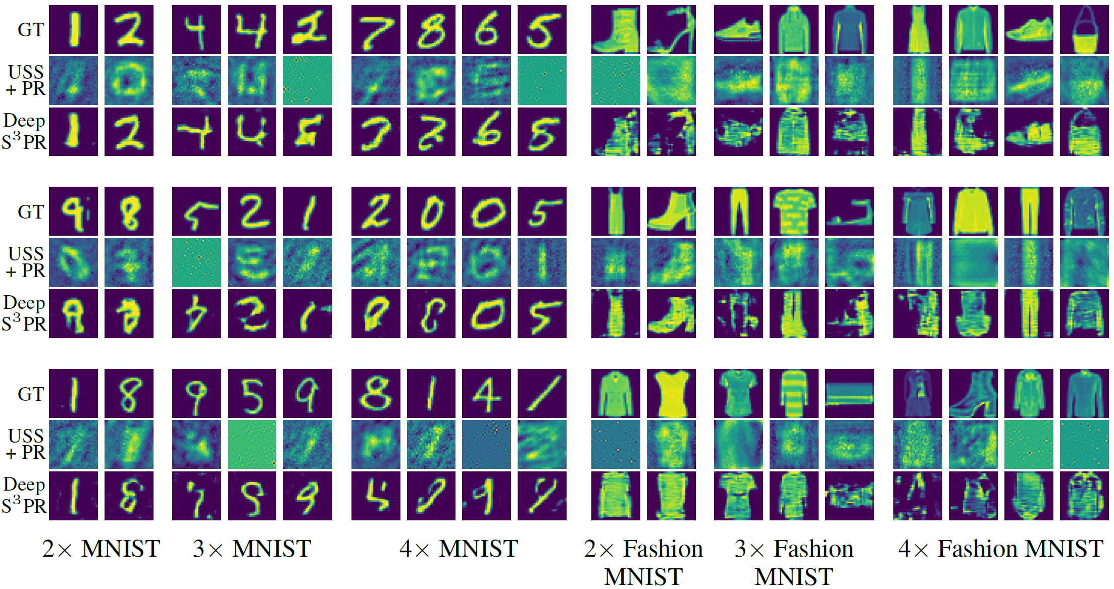
Figure 9: Fourier Measurement Matrix Results. Top: Ground truth. Middle: USS+PR reconstructions. Bottom: Deep S³PR reconstructions.

Table 6: Average NMSE across 10 sets of test images with Fourier measurement matrices.

	2$\times$ MNIST	3$\times$ MNIST	4$\times$ MNIST	2$\times$ Fashion MNIST	3$\times$ Fashion MNIST	4$\times$ Fashion MNIST
USS + PR	$.60\pm.15$	$.82\pm.11$	$.78\pm.12$	$.68\pm.24$	$.82\pm.18$	$.90\pm.15$
Deep S3PR	$.18\pm.08$	$.26\pm.04$	$.29\pm.03$	$.28\pm.14$	$.40\pm.16$	$.41\pm.18$

References

- [1] R. Gerchberg, “A practical algorithm for the determination of phase from image and diffraction plane pictures,” Optik, vol. 35, p. 237, 1972.
- [2] J. Fienup, “Reconstruction of an object from the modulus of its fourier transform,” Optics letters, vol. 3, no. 1, pp. 27–29, 1978.
- [3] J. Fienup, “Phase retrieval algorithms: a comparison,” Applied optics, vol. 21, no. 15, pp. 2758–2769, 1982.
- [4] D. Griffin and J. Lim, “Signal estimation from modified short-time fourier transform,” Acoustics, Speech and Signal Processing, IEEE Transactions on, vol. 32, no. 2, pp. 236–243, 1984.
- [5] J. Zhong, L. Tian, P. Varma, and L. Waller, “Nonlinear optimization algorithm for partially coherent phase retrieval and source recovery,” IEEE Transactions on Computational Imaging, vol. 2, no. 3, pp. 310–322, 2016.
- [6] Z. Jingshan, P. Varma, L. Tian, and L. Waller, “Source shape estimation in partially coherent phase imaging with defocused intensity,” in Computational Optical Sensing and Imaging. Optical Society of America, 2015, pp. CTh1E–5.
- [7] J. Bertolotti, E. G. Van Putten, C. Blum, A. Lagendijk, W. L. Vos, and A. P. Mosk, “Non-invasive imaging through opaque scattering layers,” Nature, vol. 491, no. 7423, pp. 232–234, 2012.
- [8] O. Katz, P. Heidmann, M. Fink, and S. Gigan, “Non-invasive single-shot imaging through scattering layers and around corners via speckle correlations,” Nature photonics, vol. 8, no. 10, p. 784, 2014.
- [9] X. Li, J. A. Greenberg, and M. E. Gehm, “Single-shot multispectral imaging through a thin scatterer,” Optica, vol. 6, no. 7, pp. 864–871, 2019.
- [10] A. Viswanath, P. Rangarajan, D. MacFarlane, and M. P. Christensen, “Indirect imaging using correlography,” in Computational Optical Sensing and Imaging. Optical Society of America, 2018, pp. CM2E–3.
- [11] C. A. Metzler, F. Heide, P. Rangarajan, M. M. Balaji, A. Viswanath, A. Veeraraghavan, and R. G. Baraniuk, “Deep-inverse correlography: towards real-time high-resolution non-line-of-sight imaging,” Optica, vol. 7, no. 1, pp. 63–71, Jan 2020. [Online]. Available: http://www.osapublishing.org/optica/abstract.cfm?URI=optica-7-1-63
- [12] B. Rajaei, E. W. Tramel, S. Gigan, F. Krzakala, and L. Daudet, “Intensity-only optical compressive imaging using a multiply scattering material and a double phase retrieval approach,” in 2016 IEEE International Conference on Acoustics, Speech and Signal Processing (ICASSP). IEEE, 2016, pp. 4054–4058.
- [13] M. Sharma, C. A. Metzler, S. Nagesh, O. Cossairt, R. G. Baraniuk, and A. Veeraraghavan, “Inverse scattering via transmission matrices: Broadband illumination and fast phase retrieval algorithms,” IEEE Transactions on Computational Imaging, 2019.
- [14] H. Hassanieh, O. Abari, M. Rodriguez, M. Abdelghany, D. Katabi, and P. Indyk, “Fast millimeter wave beam alignment,” in Proceedings of the 2018 Conference of the ACM Special Interest Group on Data Communication. ACM, 2018, pp. 432–445.
- [15] H. Xiao, K. Rasul, and R. Vollgraf, “Fashion-mnist: a novel image dataset for benchmarking machine learning algorithms,” arXiv preprint arXiv:1708.07747, 2017.
- [16] M. Pfeifer, G. Williams, I. Vartanyants, R. Harder, and I. Robinson, “Three-dimensional mapping of a deformation field inside a nanocrystal,” Nature, vol. 442, no. 7098, pp. 63–66, 2006.
- [17] J. Rodriguez, R. Xu, C. Chen, Y. Zou, and J. Miao, “Oversampling smoothness: an effective algorithm for phase retrieval of noisy diffraction intensities,” Journal of applied crystallography, vol. 46, no. 2, pp. 312–318, 2013.
- [18] E. Candes, T. Strohmer, and V. Voroninski, “Phaselift: Exact and stable signal recovery from magnitude measurements via convex programming,” Communications on Pure and Applied Mathematics, vol. 66, no. 8, pp. 1241–1274, 2013.
- [19] E. Candes, X. Li, and M. Soltanolkotabi, “Phase retrieval via wirtinger flow: Theory and algorithms,” IEEE Transactions on Information Theory, vol. 61, no. 4, pp. 1985–2007, 2015.
- [20] T. Goldstein and C. Studer, “Phasemax: Convex phase retrieval via basis pursuit,” arXiv preprint arXiv:1610.07531, 2016.
- [21] S. Bahmani and J. Romberg, “Phase retrieval meets statistical learning theory: A flexible convex relaxation,” in Artificial Intelligence and Statistics, 2017, pp. 252–260.
- [22] R. Chandra, C. Studer, and T. Goldstein, “Phasepack: A phase retrieval library,” arXiv preprint arXiv:1711.10175, 2017.
- [23] M. L. Moravec, J. K. Romberg, and R. G. Baraniuk, “Compressive phase retrieval,” in Optical Engineering+ Applications. International Society for Optics and Photonics, 2007, pp. 670 120–670 120.
- [24] S. Mukherjee and C. S. Seelamantula, “An iterative algorithm for phase retrieval with sparsity constraints: application to frequency domain optical coherence tomography,” in 2012 IEEE International Conference on Acoustics, Speech and Signal Processing (ICASSP). IEEE, 2012, pp. 553–556.
- [25] P. Schniter and S. Rangan, “Compressive phase retrieval via generalized approximate message passing,” IEEE Transactions on Signal Processing, vol. 63, no. 4, pp. 1043–1055, 2015.
- [26] A. Tillmann, Y. Eldar, and J. Mairal, “Dolphin-dictionary learning for phase retrieval,” IEEE Transactions on Signal Processing, vol. 64, no. 24, pp. 6485–6500, 2016.
- [27] C. Metzler, A. Maleki, and R. Baraniuk, “BM3D-PRGAMP: Compressive phase retrieval based on BM3D denoising,” in 2016 IEEE International Conference on Image Processing (ICIP). IEEE, 2016, pp. 2504–2508.
- [28] J.-L. Chern, C.-C. Li, and S.-H. Tseng, “Blind phase retrieval and source separation of electromagnetic fields,” Optics letters, vol. 27, no. 2, pp. 89–91, 2002.
- [29] Y. Guo, A. Wang, and W. Wang, “Multi-source phase retrieval from multi-channel phaseless stft measurements,” Signal Processing, vol. 144, pp. 36–40, 2018.
- [30] Y. Guo, T. Wang, J. Li, A. Wang, and W. Wang, “Multiple input single output phase retrieval,” Circuits, Systems, and Signal Processing, pp. 1–23, 2019.
- [31] Y. Guo, X. Zhao, J. Li, A. Wang, and W. Wang, “Blind multiple input multiple output image phase retrieval,” IEEE Transactions on Industrial Electronics, 2019.
- [32] D. J. Kane, “Principal components generalized projections: a review,” JOSA B, vol. 25, no. 6, pp. A120–A132, 2008.
- [33] T. Bendory, D. Edidin, and Y. C. Eldar, “Blind phaseless short-time fourier transform recovery,” IEEE Transactions on Information Theory, 2019.
- [34] L. Molgedey and H. G. Schuster, “Separation of a mixture of independent signals using time delayed correlations,” Physical review letters, vol. 72, no. 23, p. 3634, 1994.
- [35] P. Comon, “Independent component analysis, a new concept?” Signal processing, vol. 36, no. 3, pp. 287–314, 1994.
- [36] P. Comon and C. Jutten, Handbook of Blind Source Separation: Independent component analysis and applications. Academic press, 2010.
- [37] P. Bofill and M. Zibulevsky, “Underdetermined blind source separation using sparse representations,” Signal processing, vol. 81, no. 11, pp. 2353–2362, 2001.
- [38] Y. Li, A. Cichocki, and S.-i. Amari, “Analysis of sparse representation and blind source separation,” Neural computation, vol. 16, no. 6, pp. 1193–1234, 2004.
- [39] I. Takigawa, M. Kudo, and J. Toyama, “Performance analysis of minimum -norm solutions for underdetermined source separation,” IEEE transactions on signal processing, vol. 52, no. 3, pp. 582–591, 2004.
- [40] Y. Li, S.-I. Amari, A. Cichocki, D. W. Ho, and S. Xie, “Underdetermined blind source separation based on sparse representation,” IEEE Transactions on signal processing, vol. 54, no. 2, pp. 423–437, 2006.
- [41] A. Levin and Y. Weiss, “User assisted separation of reflections from a single image using a sparsity prior,” IEEE Transactions on Pattern Analysis and Machine Intelligence, vol. 29, no. 9, pp. 1647–1654, 2007.
- [42] L. Drumetz, T. R. Meyer, J. Chanussot, A. L. Bertozzi, and C. Jutten, “Hyperspectral image unmixing with endmember bundles and group sparsity inducing mixed norms,” IEEE Transactions on Image Processing, vol. 28, no. 7, pp. 3435–3450, 2019.
- [43] A. Deleforge and Y. Traonmilin, “Phase unmixing: Multichannel source separation with magnitude constraints,” in 2017 IEEE International Conference on Acoustics, Speech and Signal Processing (ICASSP). IEEE, 2017, pp. 161–165.
- [44] Q. Fan, J. Yang, G. Hua, B. Chen, and D. Wipf, “A generic deep architecture for single image reflection removal and image smoothing,” in Proceedings of the IEEE International Conference on Computer Vision, 2017, pp. 3238–3247.
- [45] X. Zhang, R. Ng, and Q. Chen, “Single image reflection separation with perceptual losses,” in Proceedings of the IEEE Conference on Computer Vision and Pattern Recognition, 2018, pp. 4786–4794.
- [46] Y. Luo and N. Mesgarani, “Conv-tasnet: Surpassing ideal time–frequency magnitude masking for speech separation,” IEEE/ACM transactions on audio, speech, and language processing, vol. 27, no. 8, pp. 1256–1266, 2019.
- [47] A. Bora, A. Jalal, E. Price, and A. G. Dimakis, “Compressed sensing using generative models,” in Proceedings of the 34th International Conference on Machine Learning-Volume 70. JMLR. org, 2017, pp. 537–546.
- [48] A. Manoel, F. Krzakala, M. Mézard, and L. Zdeborová, “Multi-layer generalized linear estimation,” in 2017 IEEE International Symposium on Information Theory (ISIT). IEEE, 2017, pp. 2098–2102.
- [49] V. Shah and C. Hegde, “Solving linear inverse problems using gan priors: An algorithm with provable guarantees,” in 2018 IEEE International Conference on Acoustics, Speech and Signal Processing (ICASSP). IEEE, 2018, pp. 4609–4613.
- [50] Y. Wu, M. Rosca, and T. Lillicrap, “Deep compressed sensing,” in International Conference on Machine Learning, 2019, pp. 6850–6860.
- [51] P. Pandit, M. Sahraee-Ardakan, S. Rangan, P. Schniter, and A. K. Fletcher, “Inference with deep generative priors in high dimensions,” arXiv preprint arXiv:1911.03409, 2019.
- [52] F. Latorre, V. Cevher et al., “Fast and provable admm for learning with generative priors,” in Advances in Neural Information Processing Systems, 2019, pp. 12 004–12 016.
- [53] M. Dhar, A. Grover, and S. Ermon, “Modeling sparse deviations for compressed sensing using generative models,” arXiv preprint arXiv:1807.01442, 2018.
- [54] S. A. Hussein, T. Tirer, and R. Giryes, “Image-adaptive gan based reconstruction,” arXiv preprint arXiv:1906.05284, 2019.
- [55] M. Asim, A. Ahmed, and P. Hand, “Invertible generative models for inverse problems: mitigating representation error and dataset bias,” arXiv preprint arXiv:1905.11672, 2019.
- [56] P. Hand, O. Leong, and V. Voroninski, “Phase retrieval under a generative prior,” in Advances in Neural Information Processing Systems, 2018, pp. 9136–9146.
- [57] F. Shamshad and A. Ahmed, “Robust compressive phase retrieval via deep generative priors,” arXiv preprint arXiv:1808.05854, 2018.
- [58] R. Hyder, V. Shah, C. Hegde, and M. S. Asif, “Alternating phase projected gradient descent with generative priors for solving compressive phase retrieval,” in ICASSP 2019-2019 IEEE International Conference on Acoustics, Speech and Signal Processing (ICASSP). IEEE, 2019, pp. 7705–7709.
- [59] F. Shamshad, F. Abbas, and A. Ahmed, “Deep ptych: Subsampled fourier ptychography using generative priors,” in ICASSP 2019-2019 IEEE International Conference on Acoustics, Speech and Signal Processing (ICASSP). IEEE, 2019, pp. 7720–7724.
- [60] F. Shamshad, A. Hanif, F. Abbas, M. Awais, and A. Ahmed, “Adaptive ptych: Leveraging image adaptive generative priors for subsampled fourier ptychography,” in Proceedings of the IEEE International Conference on Computer Vision Workshops, 2019, pp. 0–0.
- [61] D. Ulyanov, A. Vedaldi, and V. Lempitsky, “Deep image prior,” in Proceedings of the IEEE Conference on Computer Vision and Pattern Recognition, 2018, pp. 9446–9454.
- [62] G. Jagatap and C. Hegde, “Phase retrieval using untrained neural network priors,” in NeurIPS 2019 Workshop on Solving Inverse Problems with Deep Networks, 2019.
- [63] E. Bostan, R. Heckel, M. Chen, M. Kellman, and L. Waller, “Deep phase decoder: self-calibrating phase microscopy with an untrained deep neural network,” Optica, vol. 7, no. 6, pp. 559–562, 2020.
- [64] P. Hand and B. Joshi, “Global guarantees for blind demodulation with generative priors,” arXiv preprint arXiv:1905.12576, 2019.
- [65] M. Asim, F. Shamshad, and A. Ahmed, “Blind image deconvolution using deep generative priors,” arXiv preprint arXiv:1802.04073, 2018.
- [66] B. Aubin, B. Loureiro, A. Maillard, F. Krzakala, and L. Zdeborová, “The spiked matrix model with generative priors,” in Advances in Neural Information Processing Systems, 2019, pp. 8364–8375.
- [67] Q. Kong, Y. Xu, W. Wang, P. J. Jackson, and M. D. Plumbley, “Single-channel signal separation and deconvolution with generative adversarial networks,” in Proceedings of the 28th International Joint Conference on Artificial Intelligence. AAAI Press, 2019, pp. 2747–2753.
- [68] Y. Gandelsman, A. Shocher, and M. Irani, “”double-dip”: Unsupervised image decomposition via coupled deep-image-priors,” in The IEEE Conference on Computer Vision and Pattern Recognition (CVPR), June 2019.
- [69] M. Aharon, M. Elad, and A. Bruckstein, “K-svd: An algorithm for designing overcomplete dictionaries for sparse representation,” IEEE Transactions on signal processing, vol. 54, no. 11, pp. 4311–4322, 2006.
- [70] Y. C. Pati, R. Rezaiifar, and P. S. Krishnaprasad, “Orthogonal matching pursuit: Recursive function approximation with applications to wavelet decomposition,” in Proceedings of 27th Asilomar conference on signals, systems and computers. IEEE, 1993, pp. 40–44.
- [71] D. P. Kingma and J. Ba, “Adam: A method for stochastic optimization,” arXiv preprint arXiv:1412.6980, 2014.
- [72] A. Radford, L. Metz, and S. Chintala, “Unsupervised representation learning with deep convolutional generative adversarial networks,” arXiv preprint arXiv:1511.06434, 2015.
- [73] E. Linder-Norén, “Pytorch generative adversarial networks,” https://github.com/eriklindernoren/PyTorch-GAN, 2018, accessed: 2020-1-14.
- [74] E. Candes, X. Li, and M. Soltanolkotabi, “Phase retrieval from coded diffraction patterns,” Applied and Computational Harmonic Analysis, vol. 39, no. 2, pp. 277–299, 2015.
- [75] J. Miao, P. Charalambous, J. Kirz, and D. Sayre, “Extending the methodology of x-ray crystallography to allow imaging of micrometre-sized non-crystalline specimens,” Nature, vol. 400, no. 6742, p. 342, 1999.
- [76] A. M. Maiden, M. J. Humphry, F. Zhang, and J. M. Rodenburg, “Superresolution imaging via ptychography,” JOSA A, vol. 28, no. 4, pp. 604–612, 2011.
- [77] M. Elbaum, M. King, and M. Greenebaum, “Laser correlography: transmission of high-resolution object signatures through the turbulent atmosphere,” RIVERSIDE RESEARCH INST NEW YORK, Tech. Rep., 1974.
- [78] A. Labeyrie, “Attainment of diffraction limited resolution in large telescopes by fourier analysing speckle patterns in star images,” Astron. Astrophys., vol. 6, no. 1, pp. 85–87, 1970.
- [79] I. Freund, M. Rosenbluh, and S. Feng, “Memory effects in propagation of optical waves through disordered media,” Physical review letters, vol. 61, no. 20, p. 2328, 1988.
- [80] J. W. Goodman, Speckle phenomena in optics: theory and applications. Roberts and Company Publishers, 2007.
- [81] D. F. Gardner, S. Divitt, and A. T. Watnik, “Ptychographic imaging of incoherently illuminated extended objects using speckle correlations,” Applied optics, vol. 58, no. 13, pp. 3564–3569, 2019.
- [82] Y. Li, Y. Xue, and L. Tian, “Deep speckle correlation: a deep learning approach toward scalable imaging through scattering media,” Optica, vol. 5, no. 10, pp. 1181–1190, 2018.