Equation of motion coupled-cluster approach for intrinsic losses in x-ray spectra

Abstract

We present an equation of motion coupled cluster approach for calculating and understanding intrinsic inelastic losses in core level x-ray absorption spectra (XAS). The method is based on a factorization of the transition amplitude in the time-domain, which leads to a convolution of an effective one-body spectrum and the core-hole spectral function. The spectral function characterizes these losses in terms of shake-up excitations and satellites, and is calculated using a cumulant representation of the core-hole Green’s function that includes non-linear corrections. The one-body spectrum also includes orthogonality corrections that enhance the XAS at the edge.

I Introduction

Calculations of x-ray absorption spectra (XAS) $\mu(\omega)$ from a deep core level of a many-electron system typically begin with Fermi’s golden rule

$$\mu(\omega)=\sum_{F}|\langle\Psi|D|\Psi_{F}\rangle|^{2}\delta(E_{F}-E_{0}-\hbar\omega),$$ (1)

where $|\Psi\rangle$ is the ground state with energy $E_{0}$, $D=\Sigma_{i}d_{i}$ is the (dipole) interaction with the x-ray field of frequency $\omega$, and the sum is over the eigenstates $|\Psi_{F}\rangle$ of the many-body Hamiltonian $H$ with energies $E_{F}$. While full calculations are generally intractable, the problem can be simplified in various ways. For example, in the determinantal ${\Delta}$SCF approach, where the initial and final many-body states are restricted to single-Slater determinants, the final states can be classified in terms of successive single-, double-, and higher $n$-tuple excitations.Liang et al. (2017); Liang and Prendergast (2019) Alternatively with Green’s function methods, the summation over final states is implicit.Lee et al. (2012); Bertsch and Lee (2014); Rehr et al. (2009) For molecular systems, for example, coupled-cluster (CC) Green’s function approaches have been developed both in energy-space,Peng and Kowalski (2016, 2018) and in real time.White and Chan (2018); Koulias et al. (2019); Arponen (1983); Kvaal (2012); Pedersen and Kvaal (2019); Nascimento and DePrince III (2017, 2016, 2019); Pigg et al. (2012); Sato et al. (2018) While these developments generally focus on accurate calculations, relatively less attention has been devoted to the analysis and understanding of many-body effects in the spectra.

Our aim here is to to address this shortcoming. To this end we introduce a real-time equation of motion coupled-cluster (EOM-CC) approach together with a cumulant representation of the core-hole Green’s function. Cumulant techniques have been used increasingly to understand correlation effects and exited states.Hedin (1999); Zhou et al. (2015) The approach provides an efficient method for calculations of inelastic losses which simplifies their analysis and can be systematically improved. A key step in our approach is a factorization of the XAS transition amplitude

$$\mu(t)=\langle\Psi|D(0)D(t)|\Psi\rangle=L(t)G_{c}(t)$$ (2)

into an effective one-body transition amplitude $L(t)$ and the core-hole Green’s function $G_{c}(t)$. This strategy is similar to that in the time-correlation approach of Nozieres and de DominicisNozieres and Dominicis (1969) and Nozieres and Combescot (NC),Nozieres and Combescot (1971) for the edge-singularity problem. As a consequence the XAS is given by a convolution of a one-electron cross-section $\mu_{1}(\omega)$ and the core-hole spectral function $A_{c}(\omega)$ obtained from the Fourier transforms of $L(t)$ and $G_{c}(t)$ respectively,

$$\mu(\omega)=\int d\omega^{\prime}\mu_{1}(\omega-\omega^{\prime})A_{c}(\omega^{\prime}).$$ (3)

The intrinsic inelastic losses due to the sudden creation of the core hole lead to shake-up effects characterized by satellite structure in the spectral function $A_{c}(\omega)$, and are directly related to x-ray photoemission spectra (XPS). The one-body spectrum $\mu_{1}(\omega)$ accounts for edge-enhancement orthogonality corrections, analogous to the prediction of Mahan.Mahan (1967) However, the present approach ignores extrinsic losses and interference which may likely decrease these effects.

In the remainder of this paper Sec. II describes the EOM-CC approach and Sec. III the application to XAS. Finally, Secs. IV and V present prototypical results for a diatomic system and a brief summary, respectively.

II EOM-CC theory

Intrinsic inelastic losses in XAS are implicit in the core-hole Green’s function $G_{c}(t)$

$$G_{c}(t)=-i\langle\Psi_{c}|e^{i(H-E_{0})t}|\Psi_{c}\rangle\theta(t).$$ (4)

Here $|\Psi_{c}\rangle=c_{c}|\Psi\rangle$ is the state of the system at $t=0+$ with a core-hole in a deep level $|c\rangle$. $H$ is the many-body Hamiltonian in the Hartree-Fock approximation, and $E_{0}$ is the ground state energy. Our approach for calculating $G_{c}(t)$ is based on the EOM-CC ansatz introduced by Schönhammer and Gunnarsson (SG),Schönhammer and Gunnarsson (1978) where $|\Psi\rangle$ and $|\Psi_{c}\rangle$ are taken to be single Slater determinants. The evolution of $|\Psi_{c}(t)\rangle$ is done by transforming to an initial value problem, and propagating according to the Schrodinger EOM $i\,\partial|\Psi_{c}(t)\rangle/\partial t=H|\Psi_{c}(t)\rangle$, where $|\Psi_{c}(0)\rangle=c_{c}|\Psi\rangle$. The time-evolved state $|\Psi_{c}(t)\rangle$ can be defined for any $t$ according to a CC ansatz

$$|\Psi_{c}(t)\rangle\equiv N_{c}(t)e^{T_{c}(t)}|\Psi_{c}\rangle.$$ (5)

For a non-interacting Hamiltonian, the CC ansatz for single-excitations is justified by the Thouless theorem.Thouless (1961) Here $N_{c}(t)$ is a normalization factor and the time-dependent CC operator $T_{c}(t)$ is defined in terms of single, double, etc., excitation creation operators $a^{\dagger}_{n}$, i.e.,

$$T_{c}(t)=\sum_{n}t_{n}(t)a^{\dagger}_{n}.$$ (6)

For example, for the singles $n=(i,a)$ and $a_{n}^{\dagger}=c^{\dagger}_{a}c_{i}$; for the doubles $n=i,j,a,b$ and $a_{n}^{\dagger}=c^{\dagger}_{a}c^{\dagger}_{b}c_{j}c_{i}$; etc. Following the CC convention, the indices $i,j$ refer to occupied, and $a,b,\dots$ to unoccupied levels of the independent particle ground state.

Next by applying the Schrodinger EOM, left multiplying by $e^{-T_{c}(t)}$, and dividing by $N(t)$ yields the coupled EOM

$$\left[\frac{i\,\partial\ln N(t)}{\partial t}+\frac{i\,\partial\,{T_{c}(t)}}{\partial t}\right]|\Psi_{c}\rangle=\bar{H}(t)|\Psi_{c}\rangle,$$ (7)

where $\bar{H}(t)=e^{-T_{c}(t)}H(t)e^{T_{c}(t)}$ is the similarity transformed Hamiltonian. On applying successive commutation relations, the expansion of $\bar{H}(t)$ terminates after two (four) terms for single-particle (two-particle) operators. Then left multiplying by $\langle\Psi|$ or $\langle n|=\langle\Psi|a_{n}$ separates the EOM as

$${i\,\partial\ln N_{c}(t)}/{\partial t} = \langle\Psi_{c}|\bar{H}(t)|\Psi_{c}\rangle,$$ (8)

$${i\,\partial\,t_{n}(t)}/{\partial t} = \langle n|\bar{H}(t)|\Psi_{c}\rangle.$$ (9)

As a result the core-hole Green’s function is given by the time-dependent normalization factor

$$G_{c}(t)=-iN_{c}(t)\langle\Psi_{c}|e^{T_{c}(t)}|\Psi_{c}\rangle e^{-iE_{0}t}\theta(t)=-iN_{c}(t)e^{-iE_{0}t}\theta(t).$$ (10)

Moreover, Eq. (8) implies that $N_{c}(t)$ is a pure exponential, so that $G_{c}(t)$ has a cumulant representation $G_{c}(t)=G_{c}^{0}(t)e^{C(t)}$, where $G_{c}^{0}(t)=-ie^{-i\epsilon_{c}t}\theta(t)$, and

$$C(t)=-i\int_{0}^{t}dt^{\prime}\,\langle\Psi_{c}|(\bar{H}(t^{\prime})-E^{\prime}_{0})|\Psi_{c}\rangle,$$ (11)

where $E^{\prime}_{0}=E_{0}-\epsilon_{c}$. $C(t)$ can also be represented in Landau form,Landau (1944) which simplifies the interpretation,

$$C(t) = \int d\omega\frac{\beta(\omega)}{\omega^{2}}[e^{i\omega t}-i\omega t-1],$$ (12)

$$\beta(\omega) = \frac{1}{\pi}{\rm Re}\int_{0}^{\infty}dt\,e^{-i\omega t}\frac{d}{dt}\langle\Psi_{c}|\bar{H}(t)|\Psi_{c}\rangle.$$ (13)

The cumulant kernel $\beta(\omega)$ accounts for the transfer of oscillator strength from the main peak to excitations at frequencies $\omega$, and the initial conditions $C(0)=C^{\prime}(0)=0$ guarantee its normalization and an invariant centroid. Next we evaluate the cumulant in Eq. (11). Our calculations are based on an approximate Hartree-Fock Hamiltonian for core-level XAS that assumes a single core-level localized at an atomic site,Langreth (1969)

$$H=\epsilon_{c}c_{c}^{\dagger}c_{c}+\sum_{p}\varepsilon_{p}c_{p}^{\dagger}c_{p}+\sum_{pq}v_{pq}^{cc}c_{c}c_{c}^{\dagger}c_{p}^{\dagger}c_{q}.$$ (14)

Here $\epsilon_{p}$ are eigenstates of the initial state one particle hamiltonian $h=\Sigma_{p}\epsilon_{p}c_{p}^{\dagger}c_{p}$ and $h^{\prime}=h+v$ is that for the final state in the presence of a core-hole potential $v$, and $c_{p}^{\dagger}$ and $c_{p}$ are electron creation and annihilation operators, respectively. In order to illustrate the approach here we restrict the CC operator $T_{c}(t)$ to single-excitations $T_{c}(t)=\Sigma_{a,i}t_{ai}(t)c_{a}^{\dagger}c_{i}$. On applying the comutation relations for $[H,T]$ with Fermion anticommutation properties, one obtains

$$\langle\Psi_{c}|(\bar{H}(t)-E^{\prime}_{0})|\Psi_{c}\rangle=\sum_{ia}v_{ia}t_{ai}(t).$$ (15)

From Eq. (9), the coefficients $t_{ai}(t)$ obey a first order non-linear differential equationSchönhammer and Gunnarsson (1978)

$$i\frac{\partial t_{ai}}{\partial t} = \langle ai|\bar{H}(t)|\Psi_{c}\rangle=v_{ai}+\sum_{b}v_{ab}t_{bi}(t)$$ (16)

$$- \sum_{j}t_{aj}(t)v_{ji}-\sum_{bj}t_{aj}(t)v_{jb}t_{bi}(t).$$

This expression can be interpreted perturbatively as a succession of first order, second order, and third order terms in the off-diagonal matrix elements of $h^{\prime}$. The leading term in the cumulant $v_{ia}t_{ia}^{1}(t)$ corresponds to linear response, and is second-order in the core-hole potential $v$. The leading amplitude $t^{1}_{ia}(t)$ can be evaluated analytically to first order, yielding $t^{1}_{ia}(t)=i({v_{ai}}/{\omega_{ai}})[e^{i\omega_{ai}t}-1]$, where $\omega_{ai}=\epsilon_{a}-\epsilon_{i}$. Inserting this result into Eq. (11), we obtain an expression for $C(t)$ valid to second order in $v$,

$$\beta(\omega)=\sum_{ia}|v_{ia}|^{2}\delta(\omega-\omega_{ia}).$$ (17)

Higher order terms can be calculated systematically and yield non-linear (NL) corrections to the cumulant.Tzavala et al. (2020); Mahan (1982) For example, the third order term can be obtained by inserting the 2nd order result above for $t^{1}$ above, and so on. For comparison we note that the core-hole spectral function can also be obtained from a determinantal approach where $G_{c}(t)=\det u_{ij}(t)$, $i,j=1,2\cdots N$, and $u_{ij}(t)=\langle\phi_{i}|\phi_{j}(t)\rangle e^{-i\epsilon_{i}t}=\langle i|e^{i(h^{\prime}-\epsilon_{i})t}|j\rangle$ are time-dependent overlap integrals.Nozieres and Combescot (1971)

III X-ray spectra

The contribution to the XAS from a deep core level $|c\rangle$ is obtained using the time-correlation function with the factorization $\mu(t)=L(t)G_{c}(t)$ in Eq. (2). The core-hole Green’s function $G_{c}$ is obtained from Eq. (10-13). Calculations of $L(t)$ can be done in various ways. One is based on coupled EOM or equivalent integral equations.Langreth (1969); Grebennikov et al. (1977); Privalov et al. (2001) Another uses the time-evolution of one particle states,Nozieres and Combescot (1971) with the overlap integrals $u_{ij}(t)$ defined above. Here we use a strategy similar to that of NC, except for the replacement of the sums over $k$ with those for the complete set of eigenstates $\kappa$ of $h^{\prime}$. Thus, defining the interaction operator for core transitions as $D=\Sigma_{\kappa}M_{c\kappa}c_{\kappa}^{\dagger}c_{c}$, where $M_{c\kappa}=\langle c|d|\kappa\rangle$, the one-body transition amplitude becomes

$$L(t) = \sum_{\kappa,\kappa^{\prime}}M^{*}_{c\kappa}M_{c\kappa^{\prime}}L_{\kappa,\kappa^{\prime}}(t),$$ (18)

$$L_{\kappa,\kappa^{\prime}}(t) = e^{i\epsilon_{\kappa}t}[u_{\kappa,\kappa^{\prime}}(t)-\sum^{occ}_{ij}u_{\kappa i}(t)u^{-1}_{ij}(t)u_{j\kappa^{\prime}}(t)].$$ (19)

The contribution to $L_{\kappa,\kappa^{\prime}}(t)$ from the first term on the right of Eq. (19) leads to the independent particle transition amplitude calculated in the presence of a core-hole $L_{0}(t)=\Sigma_{\kappa}|M_{c\kappa}|^{2}\exp(i\epsilon_{\kappa}t),$ and is consistent with the final-state rule.von Barth and Grossmann (1982) The diagonal contributions $\kappa=\kappa^{\prime}$ of the second term in (19) contains the analog of a theta function $\theta(k_{F}-k)$ that suppresses transitions to the occupied subspace $\kappa<k_{F}$. The off-diagonal contributions to $L_{\kappa,\kappa^{\prime}}(t)$ are dominated by $\kappa$ (or $\kappa^{\prime}$) $>k_{F}$ and $\kappa^{\prime}$ (or $\kappa$) $<k_{F}$, respectively. The net result can be approximated by the compact expression

$$L(t)\approx\sum_{\kappa}|\tilde{M}_{c\kappa}|^{2}e^{i\epsilon_{\kappa}t},$$ (20)

which is equivalent to that derived by Friedel,Friedel (1969) and preserves the XAS sum-rule $\int d\omega\mu(\omega)=L(0)$. Here $\tilde{M}_{c\kappa}=\langle c|d\bar{P}|\kappa\rangle$, where $\bar{P}=1-\Sigma^{N}_{i=1}|i\rangle\langle i|$ is the projection operator onto the unoccupied valence levels of the ground state. This approximation greatly simplifies the calculation of the XAS, and we have verified that it agrees well with that using Eq. (19). The additional terms $-\Sigma_{i}\langle c|d|i\rangle\langle i|\kappa\rangle$ from $\bar{P}$ are called replacement transitions. Physically, they serve to cancel transitions to the occupied levels of the initial system. To first order in perturbation theory the overlap $\langle i|\kappa\rangle\approx-v_{ik}/\omega_{ik}$ is negative for an attractive core-hole potential and $\kappa>i$. Thus they yield an intrinsic edge enhancement factor $(1+\chi_{\kappa})$ for each level $\kappa$ in the XAS where $\chi_{\kappa}\approx-2\Sigma_{i=1}^{N}(M_{ci}/M_{c\kappa})\langle i|\kappa\rangle$. While non-singular in molecular systems, this edge-enhancement effect leads to the Mahan power-law singularity in metalsMahan (1967) $\mu_{1}\sim|(\epsilon-\epsilon_{F})/\epsilon_{F}|^{-2\delta_{l}/\pi}$. Finally the XAS in Eq. (3) is obtained by convolving $\mu_{1}(\omega)$ with $A_{c}(\omega)$. For convenience we have shifted both $\mu_{1}(\omega)$ and $A_{c}(\omega)$ by the core level energy $\epsilon_{c}$, i.e. with $\omega=\epsilon-\epsilon_{c}$, so that in the absence of interactions $\mu_{1}(\omega)$ agrees with the independent particle XAS. Formally the spectral function represents the spectrum of shake-up excitations

$$A_{c}(\epsilon-\epsilon_{c})=\sum_{n}|S_{n}|^{2}\delta(\epsilon+\epsilon_{n}),$$ (21)

where $S_{n}=\langle\Psi_{c}|\Psi^{\prime}_{n}\rangle$ is an $N-1$ body overlap integral and $\epsilon_{n}=E^{\prime}_{n}-E_{0}$ is the net shake-up energy. The behavior of $A_{c}(\omega)$ leads to a significant reduction in the magnitude of the XAS near the edge. In metals it leads to an Anderson power-law singularityNozieres and Dominicis (1969) $[(\epsilon-\epsilon_{F})/\epsilon_{F})]^{\alpha}$. This effect is opposite in sign, and thus competes with the enhancement from $\mu_{1}(\omega)$.

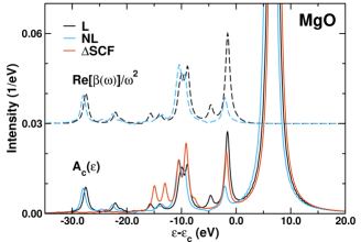
Figure 1: Cumulant kernel $\beta(\omega)$ (dashed lines) compared to the the core spectral function $A_{c}(\omega)$ (full lines) for the MgO molecule plotted vs energy relative to the bare core hole energy $\epsilon_{c}=-1334.7$ eV. Both $A_{c}(\omega)$ and $\beta(\omega)$ were calculated with either the linear (L) or non-linear (NL) approximations for $C(t)$; the $\Delta$SCF calculation was obtained from the relation $G_{c}(t)=\det u_{ij}(t)$ (see text). Note that the non-linear terms introduce a small shift of about -0.5 eV and reduce the satellite intensities.

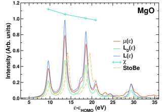
Figure 2: XAS $\mu(\omega)$ for MgO from the convolution in Eq. (3) compared to the effective one-electron XAS $L(\epsilon)=\mu_{1}(\omega)$; the independent particle XAS $L_{0}(\epsilon)=\mu_{0}(\omega)$ from the first term in Eq. (19), and from the independent electron code StoBe with a half-core-hole approximation. Also shown is the edge enhancement factor $\chi=L(\epsilon)/L_{0}(\epsilon)-1$. All spectra are shown relative to the highest occupied molecular orbital (HOMO) energy $\epsilon_{\rm HOMO}=$-8.4 eV.

IV Calculations

As an example, we present calculations for a simple diatomic molecule MgO with bond distance 1.749Å.Huber and Herzberg (retrieved January 22, 2020) We use the cc-pVDZ basis set,Prascher et al. (2011) and the parameters and associated one-particle states are obtained using a single-determinant Hartree-Fock reference. Results for the cumulant kernel $\beta(\omega)$ and the spectral function $A_{c}(\omega)$ are shown in Fig. 1. Note that the peaks in $\beta(\omega)$ correspond to the inelastic losses in the spectral function, and for MgO are dominated by shake-up excitations just below the bare core hole energy peak. These losses correspond to satellites visible in the XPS. Remarkably these results show that the non-linear terms in the cumulant are not large, so that the CC expansion converges rapidly and linear response is a good approximation. Consequently significant improvements in efficiency are possible with the CC-EOM approach. From the Landau form of the cumulant, the strength of the main peak is given by the renormalization constant $Z=\exp(-a)=0.85\ (0.88)$ for the L (NL) cases, consistent with direct integration over the main peak. Here $a=\int d\omega\,\beta(\omega)/\omega^{2}=0.16\ (0.12)$ is the net satellite strength. The quantity $\exp(-a)$ is also responsible for the amplitude reduction factor $S_{0}^{2}$ observed in the XAS fine structure.Rehr et al. (1978) We have checked that our results for $Z$ agree with those calculated using the energy-space CC Green’s function approach.Peng and Kowalski (2016, 2018) Calculations of the XAS using the cc-pVDZ basis set are also shown in Fig. 2. For comparison, we also include the XAS computed using the half core-hole approach in StoBe-deMon,Triguero et al. (1998) with a BE88PD86 exchange-correlation functionalBecke (1988); Perdew and Yue (1986) and the same basis set. Note that the StoBe-deMon results agree well with the independent particle XAS $L_{0}$. The corrections to the independent particle XAS in both $L(\epsilon)$ and $A_{c}(\epsilon)$ are substantial for MgO, but opposite in sign and dominated by the edge enhancement factor $1+\chi$. This effect can be traced to the magnitude of the core-valence matrix elements $M_{ci}$ in $\chi_{\kappa}$. Although $\chi$ exceeds unity for the bound-bound peaks near the edge, this is likely an overestimate due to the neglect of extrinsic and interference effects. On the other hand, satellite effects in the XAS are only weakly visible, e.g., in the extra peaks between about 20 and 35 eV.

V Summary and Conclusions

We have presented a real-time, EOM approach for calculations of XAS including intrinsic losses, based on the CC ansatz and a cumulant Green’s function representation of the core-hole spectral function. Although additional correlation is possible, for simplicity we have limited our treatment here to single-determinant wave-functions and the Hartree-Fock approximation. The cumulant representation facilitates both calculations and the interpretation of intrinsic losses in the spectra. A key step in our approach is a time-domain factorization leading to a convolution formula for the XAS in Eq. (2), in terms of the core-hole spectral function and an effective one-particle spectrum. These quantities account for inelastic losses due to shake up excitations, and edge enhancement corrections due to orthogonality, respectively. Though non-singular in molecular systems, both substantially affect the XAS amplitude near threshold. While extrinsic losses and interference terms due to the coupling of the photo-electron to the core-hole are ignored in this treatment, these effects are opposite in sign and tend to cancel. Remarkably the calculation of the cumulant converges rapidly, yielding good results even for the second-order or linear-response approximation. The nature of the CC-EOM cumulant is analogous to that encountered in other theoretical treatments, e.g., using the linked-cluster theorem, field-theoretic methods, or the quasi-boson approximation.Langreth (1970); Nozieres and Dominicis (1969); Hedin (1999) In condensed matter the cumulant kernel $\beta(\omega)$ is directly related to the loss function, and characterizes excitations such as density fluctuations due to the suddence appearance of the core-hole.Langreth (1970); Kas and Rehr (2017) Many extensions of the methodology introduced here are possible. For example, the treatment of emission spectra is directly analogous to that for XAS.Nozieres and Combescot (1971) A more extensive treatment including the extension to higher order CCSD excitations will be presented elsewhere.Vila et al. (2020)