$$\begin{split}\Phi(t,\rho)&=\phi_{\Delta}(t)\epsilon_{\rho}^{\Delta}\,,\\ a(t,\rho)&=1-\frac{{M}}{d-1}\epsilon_{\rho}^{d}\,,\\ b(t,\rho)&=0+{\cal O}(\epsilon_{\rho}^{2\Delta})\,.\end{split}$$ (71)

Notice that absence of boundary sources was assumed and the AdS/CFT relation $m_{\Phi}^{2}L^{2}=\Delta(\Delta-d)$ was used Witten:1998qj. Further, we used the same residual gauge freedom, as in Buchel:2012uh, to set the leading ${\cal O}(1)$ term in $b(t,\rho)$ to zero. These asymptotic conditions are valid for $\Delta>d/2$, the range of conformal dimensions that we shall consider in this work.

3.1.1 Perturbative solutions

To describe the small amplitude perturbation considered in the quantum circuit discussion, set $\Phi(t,\rho)=\varepsilon\,\Phi_{\textrm{\tiny cl}}(t,\rho)$, with $\varepsilon$ being the parameter controlling the expansion, as in eq. (LABEL:class). This induces a small amplitude expansion of the metric perturbations

$$\begin{split}a(t,\rho)&=1+\varepsilon^{2}\,a_{2}(t,\rho)+\mathcal{O}(\varepsilon^{4})\,,\\ e^{b(t,\rho)}&=1+\varepsilon^{2}\,b_{2}(t,\rho)+\mathcal{O}(\varepsilon^{4})\,,\\ \end{split}$$ (72)

which is compatible with the linearised Einstein’s equations

$$\begin{split}\partial_{\rho}a_{2}&+\frac{d-2\cos^{2}\rho}{\cos\rho\,\sin\rho}\,a_{2}=\partial_{\rho}b_{2}-\frac{m_{\Phi}^{2}L^{2}}{2(d-1)}\tan\rho\,\Phi_{\textrm{\tiny cl}}^{2}\,,\\ \partial_{\rho}b_{2}&=-\frac{1}{2(d-1)}\,\sin\rho\,\cos\rho\ \Big{(}(\partial_{\rho}\Phi_{\textrm{\tiny cl}})^{2}+(\partial_{t}\Phi_{\textrm{\tiny cl}})^{2}\Big{)}\,,\\ \partial_{t}a_{2}&=-\frac{1}{d-1}\,\sin\rho\,\cos\rho\ \partial_{\rho}\Phi_{\textrm{\tiny cl}}\,\partial_{t}\Phi_{\textrm{\tiny cl}}\,.\end{split}$$ (73)

The scalar perturbation $\Phi_{\textrm{\tiny cl}}(t,\rho)$ dynamics is controlled by the linearised KG equation, i.e., the KG equation in global AdS (LABEL:eq:gads) obtained by setting $a(t,\rho)=1$ and $b(t,\rho)=0$ in (LABEL:eq:KG)

$$\partial_{t}^{2}\Phi-\frac{1}{\tan^{d-1}\rho}\partial_{\rho}\left(\tan^{d-1}\!\rho\ \partial_{\rho}\Phi\right)+\frac{m_{\Phi}^{2}L^{2}}{\cos^{2}\rho}\,\Phi=0\,.$$ (74)

Time translation invariance of global AdS together with reality of the bulk scalar field allows to describe these perturbations as

$$\Phi_{\textrm{\tiny cl}}(t,\rho)=\sum_{j}2|\alpha_{j}|\,\cos\left(\omega_{j}t-\theta_{j}\right)\,e_{j}(\rho)\,,$$ (75)

where $\alpha_{j}=|\alpha_{j}|\,e^{i\theta_{j}}$ is the coherent state label and $e_{j}(\rho)$ are solutions to the Sturm-Liouville problem $\hat{L}[e_{j}(\rho)]=\omega_{j}^{2}e_{j}(\rho)$ with operator $\hat{L}$ given by

$$\hat{L}[e_{j}(\rho)]=-\frac{1}{\tan^{d-1}\rho}\frac{d}{d\rho}\left[\tan^{d-1}\rho\frac{d}{d\rho}e_{j}(\rho)\right]+\frac{\Delta(\Delta-d)}{\cos^{2}\rho}e_{j}(\rho)\,,$$ (76)

and $\omega_{j}=2j+\Delta$. The normalised eigenfunctions are given by

$$e_{j}(\rho)\equiv A_{j}\cos^{\Delta}\rho\,~{}{}_{2}F_{1}\left[-j,\Delta+j,\frac{d}{2};\sin^{2}\rho\right]$$ (77)

where

$$A_{j}\equiv N_{(j,0,\vec{0})}=\left(-1\right)^{j}\sqrt{\frac{16\pi G_{\textrm{\tiny N}}}{L^{d-1}}}\sqrt{\frac{\Gamma(j+\frac{d}{2})\Gamma(j+\Delta)}{j!\left[\Gamma(\frac{d}{2})\right]^{2}\Gamma(j+\Delta+1-\frac{d}{2})}}\,.$$ (78)

Due to the spherical symmetry of our perturbations, these correspond to the s-wave modes, i.e., $\ell=\vec{m}=0$, in the general discussion (LABEL:eigenwaves).

Taking into account the regularity conditions (LABEL:eq:reg) at the origin and the AdS boundary conditions (71), the first two equations in (73) can be integrated for any $\Phi_{\textrm{\tiny cl}}(t,\rho)$ yielding

$$a_{2}(t,\rho) = -\frac{1}{2(d-1)}\frac{\cos^{d}\rho}{\sin^{d-2}\rho}\int^{\rho}_{0}dy\tan^{d-1}y\Big{(}(\partial_{y}\Phi_{\textrm{\tiny cl}})^{2}+(\partial_{t}\Phi_{\textrm{\tiny cl}})^{2}+\frac{m_{\Phi}^{2}L^{2}}{\cos^{2}y}\Phi_{\textrm{\tiny cl}}^{2}\Big{)}$$ (79)

$$= -\frac{1}{d-1}\frac{\cos^{d}\rho}{\sin^{d-2}\rho}\int^{\rho}_{0}dy\tan^{d-1}y\,T^{\textrm{\tiny bulk}}_{tt}\,$$

$$b_{2}(t,\rho) = \frac{1}{2(d-1)}\int^{\pi/2}_{\rho}dy\sin y\cos y\,\Big{(}(\partial_{y}\Phi_{\textrm{\tiny cl}})^{2}+(\partial_{t}\Phi_{\textrm{\tiny cl}})^{2}\Big{)}$$ (80)

$$= \frac{1}{2(d-1)}\int^{\pi/2}_{\rho}dy\sin y\cos y\,\left(T^{\textrm{\tiny bulk}}_{tt}+T^{\textrm{\tiny bulk}}_{\rho\rho}\right)\,.$$

Notice the third equation in (73) is satisfied whenever $\Phi_{\textrm{\tiny cl}}(t,\rho)$ is on-shell. For later convenience, we have also expressed $a_{2}$ and $b_{2}$ in terms of the bulk stress tensor determined by the scalar perturbation $\Phi_{\textrm{\tiny cl}}(t,\rho)$ and sourcing the metric perturbations at second order

$$\varepsilon^{2}\,T^{\textrm{\tiny bulk}}_{\mu\nu}=-\frac{32\pi G_{\textrm{\tiny N}}}{\sqrt{|g|}}\frac{\delta I_{\textrm{\tiny matter}}}{\delta g^{\mu\nu}}=\varepsilon^{2}\left[\partial_{\mu}\Phi_{\textrm{\tiny cl}}\partial_{\nu}\Phi_{\textrm{\tiny cl}}-\frac{1}{2}g_{\mu\nu}(\partial\Phi_{\textrm{\tiny cl}}^{2}+m^{2}_{\Phi}\Phi_{\textrm{\tiny cl}}^{2})\right]\,.$$ (81)

The bulk energy density $T^{\textrm{\tiny bulk}}_{tt}$ also sources the conserved gravitational mass of these linearised solutions. Looking at the asymptotic expansion in eq. (71), the (dimensionless) mass parameter $M$ is given by

$$M=\frac{\varepsilon^{2}}{2}\int_{0}^{\pi/2}\!\!\!d\rho\tan^{d-1}\!\rho\,\left[(\partial_{t}\Phi_{\textrm{\tiny cl}})^{2}+(\partial_{\rho}\Phi_{\textrm{\tiny cl}})^{2}+\frac{m^{2}_{\Phi}L^{2}}{\cos^{2}\rho}\Phi_{\textrm{\tiny cl}}^{2}\right]=\varepsilon^{2}\int_{0}^{\pi/2}d\rho\tan^{d-1}\!\rho\ T^{\textrm{\tiny bulk}}_{tt}\,.$$ (82)

3.1.2 Wheeler-DeWitt patch

The Wheeler-DeWitt patch is a region of spacetime defined as the domain of dependence of a bulk spatial slice anchored on a Cauchy surface at the boundary $\Sigma$, i.e., typically, constant time slice. Since the complexity=action proposal (LABEL:defineCA) for holographic complexity involves evaluating the action functional on-shell over the WDW patch, the geometry of the latter is described here. This is done for global AdS $(\text{WDW})$ and for its second-order spherically symmetric perturbations $(\delta\text{WDW})$ given by

$$\begin{split}ds^{2}&=\left(g_{0,\mu\nu}+\delta g_{\mu\nu}\right)\,dy^{\mu}dy^{\nu}\\ &=\frac{L^{2}}{\cos^{2}\rho}\bigg{[}-\left(1+\varepsilon^{2}(a_{2}-2b_{2})\right)dt^{2}+\left(1-\varepsilon^{2}a_{2}\right)d\rho^{2}+\sin^{2}\rho\,d\Omega_{d-1}^{2}\bigg{]}\,.\end{split}$$ (83)

By definition, the WDW patch is bounded by a null hypersurface. Given the spherical symmetry of the geometry (83), the latter is generated by radial null geodesics emanating from the boundary surface $\Sigma$ and intersecting at the origin $\rho=0$ in a caustic. We shall distinguish between the null boundaries for global AdS $(\partial\text{WDW})$ and for the second-order perturbations $(\partial\delta\text{WDW})$.

Let us denote the boundary time picking the Cauchy surface $\Sigma$ by $t_{\Sigma}$. The past and future boundaries of the WDW patch originating at $\rho=\pi/2$ at time $t_{\Sigma}$ can be described by (see figure 3)

$$t_{\pm}(\rho)=t_{0\pm}(\rho)+\delta t_{\pm}(\rho)\,.$$ (84)

$t_{0\pm}(\rho)$ describes the undeformed past and future boundary of the WDW patch in global AdS, whereas $\delta t_{\pm}(\rho)$ describes its deformation due to the perturbation (83). Both functions are determined solving order by order the null condition

$$-\left(1+\varepsilon^{2}(a_{2}-2b_{2})\right)dt^{2}+\left(1-\varepsilon^{2}a_{2}\right)d\rho^{2}=0\,.$$ (85)

This yields

$$\begin{split}t_{0\pm}(\rho)&=t_{\Sigma}\pm\left(\frac{\pi}{2}-\rho\right)\,,\\ \delta t_{\pm}(\rho)&=\mp\,\varepsilon^{2}\int^{\pi/2}_{\rho}\Big{(}a_{2}(t_{0\pm}(y),y)-b_{2}(t_{0\pm}(y),y)\Big{)}dy\,.\end{split}$$ (86)

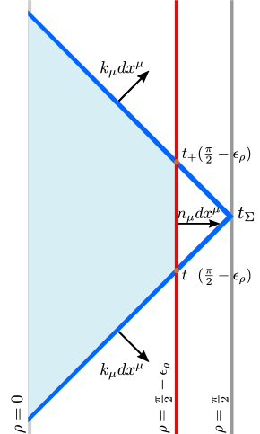
Figure 3: Representation of the WDW patch. The WDW patch is bounded by the future and past null surfaces $t_{\pm}(\rho)$ (thick blue lines) joining at $t_{\Sigma}$ on the AdS conformal boundary (grey line). $k_{\mu}dx^{\mu}$ is the outward directed normal one-form to the null WDW boundary. The regulated asymptotic AdS boundary (red line) cuts the WDW patch at $\rho=\pi/2-\epsilon_{\rho}$, and has outward directed normal $n_{\mu}dx^{\mu}$. The $\rho=\pi/2-\epsilon_{\rho}$ regulator surface and null hypersurfaces intersect at the null joint codimension-2 surfaces at $t_{\pm}(\pi/2-\epsilon_{\rho})$.

In order to evaluate the divergent action functional on the WDW patch, one needs to introduce an infinitesimal cutoff $\epsilon_{\rho}$ at the AdS boundary $\rho=\pi/2-\epsilon_{\rho}$. As depicted in figure 3, this procedure gives rise to a timelike boundary for the WDW patch, the portion of the AdS regulator surface where time runs from $t_{-}(\pi/2-\epsilon_{\rho})$ to $t_{+}(\pi/2-\epsilon_{\rho})$. This regulator surface and the null boundaries of the WDW patch intersect at the null joints, codimension-2 surfaces of constant $t=t_{\pm}(\pi/2-\epsilon_{\rho})$ and $\rho=\pi/2-\epsilon_{\rho}$ (see figure 3).

To sum up, the boundary of the WDW patch is made of the future and past null surfaces (86) together with the portion described above of the AdS regulator surface at constant $\rho=\pi/2-\epsilon_{\rho}$ and the null joints where these meet. In what follows, we introduce some geometric quantities characterizing this boundary.

We define the outward-pointing normal one-form and the corresponding null normal vector to the null WDW boundaries to be

$$\begin{split}k_{\mu}\,dx^{\mu}&\equiv(k_{0,\mu}+\delta k_{\mu})dx^{\mu}=L\left(\pm dt+d\rho-\varepsilon^{2}\left(a_{2}-b_{2}\right)d\rho\right)\,,\\ k^{\mu}\,\partial_{\mu}&\equiv(k_{0}^{\mu}+\delta k^{\mu})\partial_{\mu}=\frac{\cos^{2}\rho}{L}\left[\mp\partial_{t}+\partial_{\rho}+\varepsilon^{2}\left(\pm\left(a_{2}-2b_{2}\right)\partial_{t}+b_{2}\partial_{\rho}\right)\right]\,.\end{split}$$ (87)

The upper (lower) sign corresponds to the future (past) boundary of the WDW patch. For later convenience, we distinguished between the global AdS null normal vector $k_{0}^{\mu}$ and its $\mathcal{O}(\varepsilon^{2})$ perturbation $\delta k^{\mu}$.

We can define a null coordinate $s$ parameterizing the null translations along the WDW boundaries through $\partial_{s}\equiv k^{\mu}\partial_{\mu}$. Hence, the null hypersurface bounding the WDW patch can be conveniently parameterized by the ($d$–1)-dimensional unit sphere in (83) and the null coordinate $s$. The induced metric $\gamma$ on this null surface coincides with the angular part of the metric (83) and has no perturbative corrections. Namely

$$ds^{2}_{\partial\textrm{\tiny WDW}}=L^{2}\,\tan^{2}\!\rho\ d\Omega_{d-1}^{2}$$ (88)

with its determinant being

$$\gamma=L^{2(d-1)}\,\tan^{2(d-1)}\!\rho\,.$$ (89)

Notice the parameter $s$ is affine only at leading order in the perturbative expansion. This can be seen from explicitly evaluating

$$k^{\mu}\nabla_{\mu}k_{\nu}=\kappa\,k_{\nu}\,$$ (90)

which shows that $\kappa$ vanishes only at leading order

$$\kappa=\delta\kappa=\pm\varepsilon^{2}\frac{\cos^{2}\rho}{L}\partial_{t}(a_{2}-b_{2})\,.$$ (91)

Similarly, for the AdS regulator surface, the outward directed normal one-form and vector read n_μdx^μ &≡( n_0,μ + δn_μ )dx^μ = Lcosρ(1- ε22a_2 ) dρ 
n^μ ∂_μ ≡( n_0^ μ + δn^μ )∂_μ = cosρL(1+ ε22a_2 ) ∂_ρ . The induced metric on the AdS regulator surface equals $h_{\mu\nu}=g_{\mu\nu}-n_{\mu}n_{\nu}$. With an analogous notation as for the other geometric quantities, we will distinguish between the AdS, $h_{0,\mu\nu}$, and the perturbed part, $\delta h_{\mu\nu}$, of the metric $h_{\mu\nu}$.

Finally, the codimension-2 null joint surfaces have induced metric $\sigma$. It reduces to the angular part of the metric (83). Thus, $\sigma$ coincides with $\gamma$ and has no perturbative corrections in $\varepsilon$.

3.2 Complexity=Action

The complexity=action conjecture Brown:2015bva; Brown:2015lvg suggests the complexity of a boundary state on the time slice $\Sigma$ can be calculated holographically as the gravitational action evaluated on the Wheeler-DeWitt patch, i.e.,

$${\cal C}_{\textrm{\tiny A}}(\Sigma)=\frac{I_{\textrm{\tiny WDW}}}{\pi}\,.$$ (92)

The evaluation of the holographic complexity (92) in the purely gravitational sector requires the addition of boundary contributions to the effective action to have a well defined variational principle due to the boundaries of the WDW patch Lehner:2016vdi. Following the conventions adopted in Chapman:2018dem, the action including these gravitational boundary terms reads

$$I =I_{\textrm{\tiny bulk}}+I_{\textrm{\tiny GHY}}+I_{\textrm{\tiny jt}}+I_{\kappa}+I_{\textrm{\tiny ct}}$$ (93)

$$=\frac{1}{16\pi G_{\textrm{\tiny N}}}\int d^{d+1}y\sqrt{|g|}\bigg{[}{\cal R}+\frac{d(d-1)}{L^{2}}-\frac{1}{2}g^{\mu\nu}\nabla_{\mu}\Phi\nabla_{\nu}\Phi-\frac{1}{2}m_{\Phi}^{2}\Phi^{2}\bigg{]}$$

$$\,+\frac{1}{8\pi G_{\textrm{\tiny N}}}\int_{\textrm{\tiny regulator}}\!\!\!\!\!d^{d}x\,\sqrt{|h|}\,K+\frac{1}{8\pi G_{\textrm{\tiny N}}}\int_{\rm joints}\!\!\!\!\!d\Omega_{d-1}\,\sqrt{\sigma}\,a_{\textrm{\tiny jt}}$$

$$\,+\frac{1}{8\pi G_{\textrm{\tiny N}}}\int_{\partial{\rm WDW}}\!\!\!\!\!ds\,d\Omega_{d-1}\,\sqrt{\gamma}\,\kappa+\frac{1}{8\pi G_{\textrm{\tiny N}}}\int_{\partial{\rm WDW}}\!\!\!\!\!ds\,d\Omega_{d-1}\,\sqrt{\gamma}\,\Theta\log(\ell_{\rm ct}\Theta)\,.$$

The bulk action (LABEL:Bact)

$$I_{\textrm{\tiny bulk}}=I_{\textrm{\tiny EH}}+I_{\textrm{\tiny matter}}\,,$$ (94)

splits into $I_{\textrm{\tiny EH}}$, the Einstein-Hilbert action with a negative cosmological constant, and $I_{\textrm{\tiny matter}}$, describing the coupling of the real massive scalar field to gravity, as isolated in eq. (LABEL:eq:class-action). These match the bulk physics reviewed in section LABEL:sec:AdSsetup. The remaining terms are surface terms evaluated on the different pieces of the boundary of the WDW patch: $I_{\textrm{\tiny GHY}}$ is the usual Gibbons-Hawking-York term PhysRevLett.28.1082; PhysRevD.15.2752 defined on the AdS boundary regulator surface, $I_{\kappa}$ and $I_{\textrm{\tiny ct}}$ involve integration over the null boundaries of the WDW patch, whereas $I_{\textrm{\tiny jt}}$ is the null joint term evaluated where the null boundaries of the WDW patch intersect the AdS boundary regulator surface Lehner:2016vdi. Notice that, as for vacuum AdS solutions Chapman:2016hwi, there is no additional contribution associated to the caustics at the tips of the WDW patch (see appendix LABEL:app:caustic).

Due to the presence of $I_{\textrm{\tiny matter}}$, the first question to ask is whether the matter sector of the effective action also requires the addition of boundary contributions to preserve the well definiteness of the variational principle. To analyse this, compute the variation

$$\begin{split}\delta I_{\textrm{\tiny matter}}&=\frac{1}{16\pi G_{\textrm{\tiny N}}}\int d^{d+1}y\sqrt{|g|}\delta\Phi\left(\Box\Phi-m_{\Phi}^{2}\,\Phi\right)-\frac{1}{16\pi G_{\textrm{\tiny N}}}\int d^{d}y\sqrt{|h|}\,\delta\Phi\,n^{\mu}\partial_{\mu}\Phi\Big{|}_{\rho=\rho_{\epsilon}}\\ &-\frac{1}{16\pi G_{\textrm{\tiny N}}}\int_{\partial\textrm{\tiny WDW}}ds\,\sqrt{\gamma}\,\delta\Phi\,\partial_{s}\Phi\,.\end{split}$$ (95)

The first term is the Klein-Gordon equation of motion and vanishes on-shell. The second and third terms correspond to boundary contributions at the AdS boundary regulator surface and the null boundary of the WDW patch, respectively.

The second term is the standard one considered in AdS/CFT. In the range of conformal dimensions $\Delta>d/2$, the asymptotic expansion for the bulk scalar field (e.g., Klebanov:1999tb )

$$\Phi=\epsilon_{\rho}^{d-\Delta}\phi_{d-\Delta}+\dots+\epsilon_{\rho}^{\Delta}\phi_{\Delta}+O(\epsilon_{\rho}^{\Delta+2})$$ (96)

gives a boundary term contribution proportional to

$$\begin{split}-\int d^{d}x\sqrt{|h|}\delta\Phi n^{\mu}\partial_{\mu}\Phi&=(d-\Delta)\epsilon_{\rho}^{d-2\Delta}\phi_{d-\Delta}\delta\phi_{d-\Delta}+\dots\\ &+\left[\Delta\delta\phi_{d-\Delta}\phi_{\Delta}+(d-\Delta)\delta\phi_{\Delta}\phi_{d-\Delta}\right]+\Delta\phi_{\Delta}\delta\phi_{\Delta}\,\epsilon_{\rho}^{2\Delta+1-d}\end{split}$$ (97)

where the omitted terms are intermediate powers and functionals of the mode $\phi_{d-\Delta}$ only. Imposing Dirichlet boundary conditions with vanishing leading mode, i.e., $\delta\phi_{d-\Delta}=\phi_{d-\Delta}=0$, this boundary term vanishes when removing the cutoff.

Regarding the third term, we proceed as in the gravitational sector Lehner:2016vdi. Hence, we assume Dirichlet boundary conditions along the null boundary of the WDW patch so that $\delta\Phi=0$ in this term, i.e., we do not impose any additional boundary conditions for the bulk scalar field along the null boundary.

The discussion above indicates the existence of a good variational principle for the bulk scalar field when $\Delta>d/2$ without the addition of any further boundary contributions. This extends the argument in Lehner:2016vdi to the full effective action (93) in this range of conformal dimensions.

This result allows us to compute the variation of the holographic complexity $\delta{\cal C}_{\textrm{\tiny A}}(\Sigma)$ using eq. (92) to second order in the bulk scalar field amplitude $\varepsilon$. To organise our discussion, we split $\delta{\cal C}_{\textrm{\tiny A}}(\Sigma)$ into the three types of contributions that in principle appear

$$\delta{\cal C}_{\textrm{\tiny A}}(\Sigma)=\frac{1}{\pi}\left(\delta I_{\textrm{\tiny WDW}}+\delta I_{\delta\textrm{\tiny WDW}}+\delta I_{\delta\textrm{\tiny cutoff}}\right)\,.$$ (98)

$\delta I_{\textrm{\tiny WDW}}$ is the variation due to the change in the background fields within the original WDW patch, $\delta I_{\delta\text{WDW}}$ is the variation due to the change in the shape of the WDW patch and $\delta I_{\delta\textrm{\tiny cutoff}}$ is the variation due to the change of the radial location of the AdS boundary regulator surface.

A detailed description of the contribution from each of the terms in (93) to $\delta I_{\textrm{\tiny WDW}}$ and $\delta I_{\delta\textrm{\tiny WDW}}$ appears in the next section. We also show that in the present case $\delta I_{\delta\textrm{\tiny cutoff}}$ actually vanishes. Readers not interested in the details of their evaluation can skip to section LABEL:sec:CA-result, where the net result is summarized.

3.2.1 Action variation evaluation

In this section, we start by showing that the variation of the location of the radial cutoff has no impact on the variation of the action. We then compute the contributions to $\delta I_{\textrm{\tiny WDW}}$ and $\delta I_{\delta\textrm{\tiny WDW}}$ originating from the different terms in (93).

Variation of the cutoff $\delta I_{\delta\textrm{\tiny cutoff}}$.

Before computing $\delta I_{\textrm{\tiny WDW}}$ and $\delta I_{\delta\textrm{\tiny WDW}}$, we show the contribution $\delta I_{\delta\textrm{\tiny cutoff}}$ vanishes, to second order in the amplitude $\varepsilon$, whenever the conformal dimension $\Delta>d/2$.

The origin of $\delta I_{\delta\textrm{\tiny cutoff}}$ is the usual procedure to fix the cutoff by going to the Fefferman-Graham coordinates fefferman1985elie; fefferman2007ambient (see Emparan:1999pm; deHaro:2000vlm; Skenderis:2002wp for standard holographic renormalisation applications). In appendix LABEL:app:ads, we show the global AdS $(\epsilon_{\rho})$ and the perturbed solution $(\epsilon_{\textrm{\tiny pert}})$ cutoffs differ by an order ${\cal O}(\varepsilon^{2})$ term

$$\epsilon_{\textrm{\tiny pert}}=\epsilon_{\rho}\left(1+\frac{1}{2}\varepsilon^{2}a_{2}(t,\pi/2-\epsilon_{\rho})\right)\,.$$ (99)

Since this difference is already second order, to compute $\delta I_{\delta\textrm{\tiny cutoff}}$ reduces to evaluating (93) for global AdS integrating up to $\epsilon_{\textrm{\tiny pert}}$ (see appendix LABEL:app:ads for details)

$$I_{\textrm{\tiny vac}}=\frac{\text{Vol}\,\Omega_{d-1}L^{d-1}}{8\pi G_{\textrm{\tiny N}}}\epsilon_{\textrm{\tiny pert}}^{1-d}\left(2(d-1)-\frac{1}{d-1}+\log\frac{\ell_{\textrm{\tiny ct}}(d-1)}{L}+\dots\right)\,$$ (100)

where dots indicate subleading terms in the cutoff expansion. Using (99), this term results in an extra contribution to $\delta{\cal C}_{\textrm{\tiny A}}(\Sigma)$, which reads

$$\delta I_{\delta\textrm{\tiny cutoff}}=\frac{\varepsilon^{2}\text{Vol}\,\Omega_{d-1}L^{d-1}}{16\pi G_{\textrm{\tiny N}}}\epsilon_{\rho}^{1-d}a_{2}(t,\pi/2-\epsilon_{\rho})\left(2(d-1)^{2}-1+(d-1)\log\frac{\ell_{\textrm{\tiny ct}}(d-1)}{L}+\dots\right)\,.$$ (101)

However, given the asymptotic boundary conditions (71), it follows $a_{2}\sim\epsilon^{d}_{\rho}$. Hence, $\delta I_{\delta\textrm{\tiny cutoff}}$ vanishes linearly in the cutoff $\epsilon_{\rho}$. The corrections to $\delta I_{\textrm{\tiny WDW}}$ and $\delta I_{\delta\textrm{\tiny WDW}}$ due to (99) are higher order in the $\varepsilon$ perturbative expansion we are considering. Hence, in what follows, we will simply identify both cutoffs.

Gravitational bulk term.

To evaluate the contributions to $\delta I_{\textrm{\tiny WDW}}$ and $\delta I_{\delta\textrm{\tiny WDW}}$ we start with the variation of the Einstein-Hilbert action coupled to a cosmological constant term

$$I_{\textrm{\tiny EH}}=\frac{1}{16\pi G_{\textrm{\tiny N}}}\int d^{d+1}y\sqrt{|g|}\bigg{[}{\cal R}+\frac{d(d-1)}{L^{2}}\bigg{]}\,.$$ (102)

Following the general discussion, its second order variation splits into two contributions

$$\delta I_{\textrm{\tiny EH}}=\delta I_{\textrm{\tiny EH,\,WDW}}+\delta I_{\textrm{\tiny EH},\,\delta\textrm{\tiny WDW}}\,.$$ (103)

$\delta I_{\textrm{\tiny EH,\,WDW}}$ comes from the second order variation of the action evaluated on the undeformed WDW patch. Since the variation of the action is computed around a solution to the equations of motion, this term reduces to a total derivative

$$\delta I_{\textrm{\tiny EH,\,WDW}}=\frac{1}{16\pi G_{\textrm{\tiny N}}}\int_{\textrm{\tiny WDW}}\!\!\!\!\!d^{d+1}y\,\sqrt{|g_{0}|}\,\nabla_{\sigma}\left(g_{0}^{\sigma\nu}\nabla^{\mu}\delta g_{\mu\nu}-\nabla^{\sigma}\delta g^{\mu}_{\mu}\right)\,.$$ (104)

Notice that all covariant derivatives are vacuum AdS derivatives. Using Stokes’ theorem, $\delta I_{\textrm{\tiny EH,\,WDW}}$ is localized on the boundary of the (regulated) WDW patch

$$\begin{split}\delta I_{\textrm{\tiny EH,\,WDW}}&=\frac{1}{16\pi G_{\textrm{\tiny N}}}\int_{\partial\textrm{\tiny WDW}}\!\!\!\!ds\,d\Omega_{d-1}\,\sqrt{\gamma}\,k_{0,\sigma}\left(g_{0}^{\sigma\nu}\nabla^{\mu}\delta g_{\mu\nu}-\nabla^{\sigma}\delta g^{\mu}{}_{\mu}\right)\,\\ &~{}+\frac{1}{16\pi G_{\textrm{\tiny N}}}\int_{t_{0-}(\rho)}^{t_{0+}(\rho)\!\!\!}dt\,d\Omega_{d-1}\sqrt{|h_{0}|}n_{0,\sigma}\left(g_{0}^{\sigma\nu}\nabla^{\mu}\delta g_{\mu\nu}-\nabla^{\sigma}\delta g^{\mu}{}_{\mu}\right)\,\Bigg{|}_{\rho=\frac{\pi}{2}-\epsilon_{\rho}}\\ &\equiv\delta I_{\textrm{\tiny EH,\,null}}+\delta I_{\textrm{\tiny EH,\,reg }}\,\end{split}$$ (105)

This boundary term splits into two contributions (see figure 3): the first is evaluated on the null hypersurface $\partial$WDW up to the regulator surface. This has induced metric determinant $\gamma=L^{2(d-1)}\,\tan^{2(d-1)}\!\rho\,$ and normal one-form $k_{\sigma}$, as in (87). The second, is evaluated on the time-like regulator surface $\rho=\frac{\pi}{2}-\epsilon_{\rho}$ with induced (unperturbed) metric determinant $|h_{0}|=L^{2d}\,\tan^{2(d-1)}\!\rho/\cos^{2}\!\rho$ and normal $n_{\sigma}$ as in (3.1.2).

Substituting the explicit expressions, using integration by parts in some of the terms and taking into account the metric perturbation regularity conditions at the origin (LABEL:eq:reg) and fall-offs at the AdS boundary (71), yields for the null surface contribution δI_EH, null =& ε28 πGNL ∫_∂WDW ​​​​ds   dΩ_d-1    γ [ ∓cos^2 ρ  ∂_t (a_2-b_2) - (d-1) cotρ  b_2
- sinρcosρ(a_2 -b_2 ) ] -ε216 πGN∫_joints​​dΩ_d-1   γ ( a_2- 2b_2) where, as before, the upper (lower) sign refers to the upper (lower) part of the WDW patch boundary. The last term arises from integrating by parts, and it is evaluated at the location of the joints between the original WDW boundary and the regulator surface.

Similarly the integral along the regulator surface gives δI_EH, reg & = -ε216πGNL ∫_t_0-(ρ)^t_0+( ρ) ​​ dt   dΩ_d-1  —h_0—   [ d- cos2ρsinρ a_2
                         + sinρ(a_2- 2 b_2 ) + cosρ  ∂_ρ (a_2 - 2 b_2) ] —_ρ=π2- ϵ_ρ  .

The second contribution to $\delta I_{\textrm{\tiny EH}}$ in eq. (103) arises from the background AdS action evaluated over the geometric variation of the WDW patch described by eq. (86): δI_EH, δWDW &= 116πGN∫_δWDW ​​​​​ d^d+1y —g_0—[R_0+ d(d-1)L2]
= - d   8πGNL2 ∫dρ  dΩ_d-1 - g_0   ( δt_+ (ρ) - δt_-(ρ) )  . In writing the second line we made explicit use of the vacuum AdS_d+1 value of ${\cal R}_{0}=-d(d+1)/L^{2}$. Using the integral expression (86) for $\delta t_{\pm}(\rho)$ and rearranging the order of integration, this contribution can also be recast in the form of an integral over the boundary of the undeformed WDW

$$\begin{split}\delta I_{\textrm{\tiny EH},\,\delta\textrm{\tiny WDW}}=\frac{\varepsilon^{2}}{8\pi G_{\textrm{\tiny N}}L}\int_{\partial\textrm{\tiny WDW}}\!\!\!\!\!ds\,d\Omega_{d-1}\,\sqrt{\gamma}\,\sin\rho\cos\rho\left(a_{2}-b_{2}\right)\,.\end{split}$$ (106)

Since this cancels one of the terms in eq. (3.2.1), the complete variation $\delta I_{\textrm{\tiny EH}}$ equals δI_EH &= ε28 πGNL ∫_∂WDW ​​​​ ds dΩ_d-1 γ   [ ∓cos^2 ρ  ∂_t (a_2-b_2) - (d-1) cotρ  b_2 ] 
-ε216πGNL ∫_t_0-(ρ)^t_0+( ρ) dt   dΩ_d-1 —h_0— [ d- cos2ρsinρ a_2 + sinρ(a_2- 2 b_2) + cosρ  ∂_ρ (a_2 - 2 b_2) ] —_ρ=π2- ϵ_ρ
-ε216 πGN ∫_joints dΩ_d-1 γ ( a_2-2 b_2)
For conformal dimensions $\Delta>d/2$, both the second and third line contributions vanish when removing the cutoff $\epsilon_{\rho}$ due to the asymptotic boundary conditions (71). More concretely, the vanishing of the unit sphere integral in the joint term follows from expanding the integrand for $\epsilon_{\rho}\to 0$. Since, $\sqrt{\gamma}\sim\epsilon_{\rho}^{1-d}$, $a_{2}\sim\epsilon_{\rho}^{d}$ and $b_{2}\sim\epsilon_{\rho}^{2\Delta}$, the conclusion follows for $2\Delta>d$. The AdS regulator surface term has a constant contribution when expanding near the AdS boundary, but the integration along the time direction between $t_{0+}(\pi/2-\epsilon_{\rho})$ and $t_{0-}(\pi/2-\epsilon_{\rho})$ (see eq. (86)) yields an overall linear dependence in the cutoff for small $\epsilon_{\rho}$. Thus, in the limit where the regulator surface is removed, $\delta I_{\textrm{\tiny EH}}$ in eq. (3.2.1) reduces to

$$\delta I_{\textrm{\tiny EH}}=\frac{\varepsilon^{2}}{8\pi G_{\textrm{\tiny N}}L}\int_{\partial\textrm{\tiny WDW}}\!\!\!\!ds\,d\Omega_{d-1}\sqrt{\gamma}\,\Big{[}\mp\cos^{2}\rho\,\partial_{t}(a_{2}-b_{2})-(d-1)\cot\rho\,b_{2}\Big{]}\,.\\$$ (107)

GHY term.

The GHY term in eq. (93)

$$I_{\textrm{\tiny GHY}}=\frac{1}{8\pi G_{\textrm{\tiny N}}}\int_{\textrm{\tiny regulator}}\!\!\!\!\!\!\!\!\!d^{d}x\,\sqrt{|h|}\,K\,$$ (108)

involves the integral of the trace, $K=h^{\mu\nu}K_{\mu\nu}$, of the extrinsic curvature $K_{\mu\nu}=h_{~{}\mu}^{\sigma}h_{~{}\nu}^{\rho}\,\nabla_{\sigma}n_{\rho}$ of the asymptotic regulator surface $\rho=\pi/2-\epsilon_{\rho}$, where the WDW patch gets cut off Carmi:2016wjl. Here $n_{\rho}$ is the outward directed normal to the regulator surface – see eq. (3.1.2).

Following the general discussion around eq. (98), the second order variation $\delta I_{\textrm{\tiny GHY}}$ involves two contributions

$$\delta I_{\textrm{\tiny GHY}}=\delta I_{\textrm{\tiny GHY},\,\textrm{\tiny WDW}}+\delta I_{\textrm{\tiny GHY},\,\delta\textrm{\tiny WDW}}\,.$$ (109)

$\delta I_{\textrm{\tiny GHY},\,\textrm{\tiny WDW}}$ comes from integrating the second order variation of $\sqrt{|h|}\,K$ along the segment of the AdS regulator surface intersecting the original WDW patch (see figure 3)

$$\begin{split}\delta I_{\textrm{\tiny GHY},\,\textrm{\tiny WDW}}&=\frac{1}{8\pi G_{\textrm{\tiny N}}}\int_{t_{0-}(\rho)}^{t_{0+}(\rho)\!\!\!}dt\,d\Omega_{d-1}\sqrt{|h_{0}|}\Big{[}\frac{1}{2}K_{0}\,h_{0}^{\mu\nu}\delta h_{\mu\nu}+\delta K\Big{]}\Bigg{|}_{\rho=\frac{\pi}{2}-\epsilon_{\rho}}\\ &=\frac{1}{16\pi G_{\textrm{\tiny N}}}\int_{t_{0-}(\rho)}^{t_{0+}(\rho)\!\!\!}dt\,d\Omega_{d-1}\sqrt{|h_{0}|}\Big{[}K_{0}\,h_{0}^{\mu\nu}\delta h_{\mu\nu}-K_{0}^{\mu\nu}\delta g_{\mu\nu}\\ &\hskip 170.71652pt-n_{0}^{\nu}\left(\nabla^{\mu}\delta g_{\mu\nu}-\nabla_{\nu}\delta g^{\mu}{}_{\mu}\right)\Big{]}\Bigg{|}_{\rho=\frac{\pi}{2}-\epsilon_{\rho}}\,.\end{split}$$ (110)

Following the notation used so far, $K_{0}$ indicates the AdS value of the extrinsic curvature and $\delta K$ its second order variation. In writing the second expression we have used (see e.g., usefulformulas)

$$\delta K=-\frac{1}{2}K_{0}^{\mu\nu}\delta g_{\mu\nu}-\frac{1}{2}n_{0,\sigma}\left(g_{0}^{\sigma\nu}\nabla^{\mu}\delta g_{\mu\nu}-\nabla^{\sigma}\delta g^{\mu}{}_{\mu}\right)+\mathcal{D}_{\mu}c^{\mu}\,$$ (111)

and the fact that $c_{\mu}=-\frac{1}{2}h^{\,~{}~{}\sigma}_{0,\mu}n_{0}^{\nu}\delta g_{\sigma\nu}$ identically vanishes (here $\mathcal{D}_{\mu}$ is the covariant derivative on the regulator surface compatible with the induced metric).

$\delta I_{\textrm{\tiny GHY},\,\delta\textrm{\tiny WDW}}$ involves the background value $\sqrt{|h_{0}|}\,K_{0}$ evaluated over the intersection between the deformation of the WDW patch and the regulator surface

$$\delta I_{\textrm{\tiny GHY},\,\delta\textrm{\tiny WDW}}=\frac{1}{8\pi G_{\textrm{\tiny N}}}\int d\Omega_{d-1}\sqrt{|h_{0}|}K_{0}\Big{(}\delta t_{+}(\rho)-\delta t_{-}(\rho)\Big{)}\Bigg{|}_{\rho=\frac{\pi}{2}-\epsilon_{\rho}}\,.$$ (112)

Explicit calculation gives rise to δI_GHY , WDW = ε28πGNL ∫_t_0-(ρ)^t_0+( ρ) dt   dΩ_d-1 —h_0— ( d- cos2ρsinρ (a_2 - b_2) + cosρ2 ∂_ρ (a_2 - 2b_2) ) —_ρ=π2- ϵ_ρ and δI