HATS-47b, HATS-48Ab, HATS-49b and HATS-72b: Four Warm Giant Planets Transiting K Dwarfs

Abstract

We report the discovery of four transiting giant planets around K dwarfs. The planets HATS-47b, HATS-48Ab, HATS-49b, and HATS-72b have masses of $0.369_{-0.021}^{+0.031}$ $M_{\rm J}$, $0.243_{-0.030}^{+0.022}$ $M_{\rm J}$, $0.353_{-0.027}^{+0.038}$ $M_{\rm J}$ and $0.1254\pm 0.0039$ $M_{\rm J}$, respectively, and radii of $1.117\pm 0.014$ $R_{\rm J}$, $0.800\pm 0.015$ $R_{\rm J}$, $0.765\pm 0.013$ $R_{\rm J}$, and $0.7224\pm 0.0032$ $R_{\rm J}$, respectively. The planets orbit close to their host stars with orbital periods of $3.9228$ d, $3.1317$ d, $4.1480$ d and $7.3279$ d, respectively. The hosts are main sequence K dwarfs with masses of $0.674_{-0.012}^{+0.016}$ $M_{\sun}$, $0.7279\pm 0.0066$ $M_{\sun}$, $0.7133\pm 0.0075$ $M_{\sun}$, and $0.7311\pm 0.0028$, and with $V$-band magnitudes of $V=14.829\pm 0.010$, $14.35\pm 0.11$, $14.998\pm 0.040$ and $12.469\pm 0.010$. The Super-Neptune HATS-72b (a.k.a. WASP-191b and TOI 294.01) was independently identified as a transiting planet candidate by the HATSouth, WASP and TESS surveys, and we present a combined analysis of all of the data gathered by each of these projects (and their follow-up programs). An exceptionally precise mass is measured for HATS-72b thanks to high-precision radial velocity (RV) measurements obtained with VLT/ESPRESSO, FEROS, HARPS and Magellan/PFS. We also incorporate TESS observations of the warm Saturn-hosting systems HATS-47 (a.k.a. TOI 1073.01), HATS-48A and HATS-49. HATS-47 was independently identified as a candidate by the TESS team, while the other two systems were not previously identified from the TESS data. The RV orbital variations are measured for these systems using Magellan/PFS. HATS-48A has a resolved $5\farcs 4$ neighbor in Gaia DR2, which is a common-proper-motion binary star companion to HATS-48A with a mass of $0.22$ $M_{\sun}$ and a current projected physical separation of $\sim$1,400 au.

1 Introduction

Much of our empirical knowledge about the physical properties of planets beyond the Solar System (exoplanets) comes from observing planets with orbits that are fortuitously oriented such that the planets transit in front of their host stars from our vantage point.

Of particular importance are transiting planets with masses that have been measured either via high-precision radial velocity (RV) observations (e.g., Henry et al., 2000; Charbonneau et al., 2000; Konacki et al., 2003), or by observing deviations from strict periodicity in the transit times of other planets in the planetary system (e.g., Holman et al., 2010). Measuring both the planetary mass and radius (the latter being measurable from the transits once the physical properties of the host star are determined), together with the incident stellar flux (determined from the period once the stellar luminosity and mass are known) and system age (determined as one of the host star properties), allows constraints to be set on the composition of the planet (e.g., Guillot et al., 2006). The necessary stellar properties can be determined by comparing photometric, astrometric, and spectroscopic observations of the star to empirical or theoretical relations between stellar physical and observable parameters.

To date, more than 3,000 transiting planets have been confirmed or validated.. About 90% of these were found by the NASA Kepler mission (Borucki et al., 2010), or its successor K2 (Howell et al., 2014). However, the planetary masses have not yet been measured for the majority of these. Of the $\sim 600$ transiting planets with measured masses, only about one-third were discovered by Kepler or K2. The masses of typical Kepler and K2 transiting planets are difficult to measure because the planets are too small, have periods that are too long, or are orbiting stars that are too faint for effective RV monitoring.

In order to increase the number of exoplanets — particularly planets smaller than Neptune — with measured masses, NASA launched the TESS space-based photometer (Ricker et al., 2015). For its primary mission, TESS is carrying out a two-year survey of approximately three-quarters of the sky to find transiting planets around bright stars. As of the time of writing, the mission has been operational for a year and a half, and has led to the identification of about 1,000 transiting planet candidates, of which 17 new planets have so far been confirmed and have had their masses measured. The follow-up observations needed to confirm and characterize the transiting planet candidates identified by TESS are being carried out by the community, with organization provided by the TESS Follow-up Program (TFOP; Collins et al., 2018).

Approximately half of the transiting planets with measured masses were discovered by wide-field ground-based transit surveys, especially the WASP (Pollacco et al., 2006), HAT (Bakos et al., 2004, 2013) and KELT (Pepper et al., 2007, 2012) projects. These projects have primarily been sensitive to short-period gas-giant planets. They have discovered the majority of exoplanets that have been the subject of observational studies of the planetary atmospheres, and measurements of the stellar-spin–planetary-orbit alignment. These projects, some of which have been in operation for more than a decade, are now contributing to the follow-up and confirmation of transiting planets from the TESS mission. This includes both providing photometric observations carried out with the ground-based transit survey instruments, and follow-up spectroscopic and photometric observations using facilities, procedures and teams that were originally brought together to confirm candidates from the ground-based surveys.

Many of the transiting giant planet candidates detected by TESS had already been identified by the ground-based projects. Some are confirmed and published planets, some have already been ruled out as false positives, some have been confirmed but not yet published (including two cases presented in this paper), some have survived initial follow-up vetting observations but are not yet confirmed, and some have simply not been followed-up yet. There are also cases in which objects that were selected as candidates by the ground-based surveys have not been identified publicly by the TESS team. Many of these latter objects are false alarms. However, in some cases the transiting planets have been confirmed, and the reason they were not identified by TESS is that the signals are weak due to crowding, substantial scattered light, or other issues. In other cases, the candidates are around stars that are fainter than the magnitude thresholds being applied by the TESS team in searching for transit signals. Two of the planets presented in this paper have stars that are fainter than the magnitude limits currently being searched with the standard TESS procedures.

In this paper we present the discovery and characterization — including precise mass measurements — of four giant planets transiting K dwarf stars. The four planets HATS-47b, HATS-48Ab, HATS-49b and HATS-72b were identified by the HATSouth transit survey, and one was also independently identified by the WASP survey. All four of these objects also have transits that can be detected using TESS data, but only two of them have been selected as candidate transiting planet systems by the TESS team. The planets have masses between $0.1254\pm 0.0039$ $M_{\rm J}$ (HATS-72b) and $0.369_{-0.021}^{+0.031}$ $M_{\rm J}$ (HATS-47b), radii between $0.7224\pm 0.0032$ $R_{\rm J}$ (HATS-72b) and $1.117\pm 0.014$ $R_{\rm J}$ (HATS-47b), and orbit stars with masses between $0.674_{-0.012}^{+0.016}$ $M_{\sun}$ (HATS-47) and $0.7311\pm 0.0028$ $M_{\sun}$ (HATS-72). Thanks to the relatively low masses and luminosities of these host stars, the planets can all be classified as “warm” giant planets rather than “hot” giant planets: in all four cases, the expected equilibrium temperature computed under the assumptions of zero albedo and isotropic reradiation, is below 1,000 K. While hot giant planets exhibit a radius inflation anomaly (e.g., Hartman et al., 2011, among many other examples), warm giant planets are observed to have radii that are consistent with theoretical expectations (e.g., Kovács et al., 2010). More recently, Sestovic et al. (2018) have argued that planets with masses $M_{p}<0.37$ $M_{\rm J}$, which includes all the planets here, do not exhibit anomalous radius inflation, even when highly irradiated. As a result, it is reasonable to suppose that meaningful inferences about the bulk planet metal content can be derived for these warm giant planets (e.g., Thorngren et al., 2016). This makes warm low-mass giant planets, like those presented here, particularly useful for testing theories of giant planet formation and structure.

In the following section we discuss the observations used to detect, confirm and characterize the transiting planet systems HATS-47, HATS-48A, HATS-49, and HATS-72. The analysis of these data is described in Section 3. We discuss the results in Section 4.

2 Observations

Figures 1, 2, 3 and 4 show some of the observations collected for HATS-47, HATS-48A, HATS-49 and HATS-72, respectively. Each figure shows the HATSouth light curve used to detect the transits, the ground-based follow-up transit light curves, the high-precision RVs and spectral line bisector spans (BSs), and the catalog broad-band photometry, including parallax corrections from Gaia DR2 (Gaia Collaboration et al., 2018), used in characterizing the host stars. We also show the TESS light curves for each system in Figures 5, 6, 7 and 8, and the WASP light curve for HATS-72 in Figure 9. Below we describe the observations of these objects that were collected and analyzed here.

2.1 Photometric detection

All four of the systems presented here were detected as transiting planet candidates by the HATSouth ground-based transiting planet survey (Bakos et al., 2013) as we discuss in Section 2.1.1. The transits of all four objects are also detected in time-series observations collected by the TESS mission (Section 2.1.2), and HATS-47b and HATS-72b were independently identified as transiting planet candidates by the TESS team based on these data. The transits of HATS-72b were also independently identified by the WASP project, as discussed in Section 2.1.3.

2.1.1 HATSouth

HATSouth uses a network of 24 telescopes, each 0.18 m in aperture, and 4K$\times$4K front-side-illuminated CCD cameras. These are attached to a total of six fully-automated mounts, each with an associated enclosure, which are in turn located at three sites around the Southern hemisphere. The three sites are Las Campanas Observatory (LCO) in Chile, the site of the H.E.S.S. gamma-ray observatory in Namibia, and Siding Spring Observatory (SSO) in Australia. The operations and observing procedures of the network were described by Bakos et al. (2013), while the method for reducing the images to trend-filtered light curves and searching for candidate transiting planets were described by Penev et al. (2013). We note that the trend-filtering makes use of the Trend-Filtering Algorithm (TFA) of Kovács et al. (2005), while transit signals are detected using the Box-fitting Least Squares (BLS) method of Kovács et al. (2002). The HATSouth observations of each system are summarized in Table 1, and displayed in Figures 1, 2, 3, and 4, while the light curve data are made available in Table 2.

We also searched the HATSouth light curves for other periodic signals using the Generalized Lomb-Scargle method (GLS; Zechmeister & Kürster, 2009), and for additional transit signals by applying a second iteration of BLS. Both of these searches were performed on the residual light curves after subtracting the best-fit transit models.

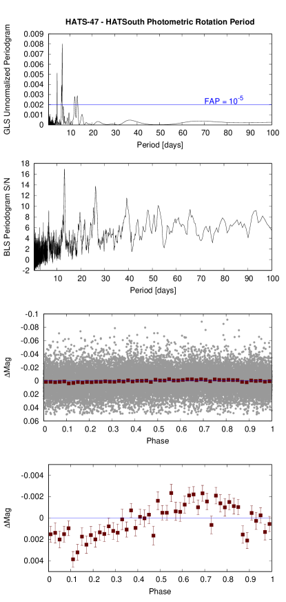
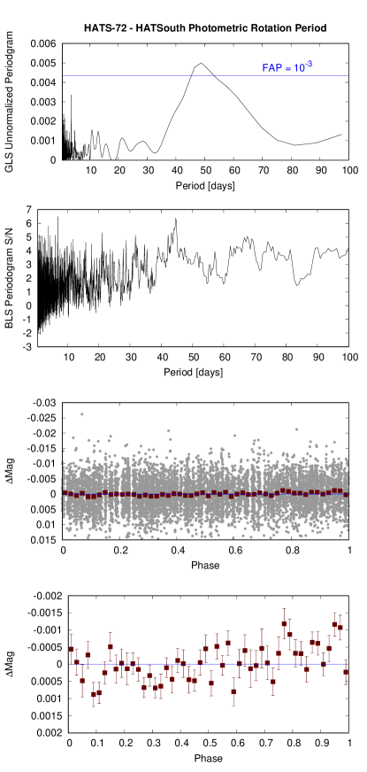
Figure 10: Detection of a strong $P=6.621581\pm 0.000078$ days photometric rotation period signal in the HATSouth light curve of HATS-47 (left) and a tentative $P=48.725\pm 0.015$ days signal in the HATSouth light curve of HATS-72 (right). In each case we show the following panels. Top: the Generalized Lomb-Scargle (GLS) periodogram of the combined HATSouth light curve after subtracting the best-fit transit model. The horizontal blue line shows the bootstrap-calibrated $10^{-5}$ false alarm probability level for HATS-47 and the $10^{-3}$ false alarm probability level for HATS-72. Second from top: The Box-fitting Least Squares (BLS) periodogram of the same light curve. For HATS-47 there is a peak in the BLS periodogram at twice the period of the strongest peak in the GLS periodogram. For HATS-72 no significant peak is present in the BLS periodogram. Second from bottom: The HATSouth light curve phase-folded at the peak GLS period. The gray points show the individual photometric measurements, while the dark red filled squares show the observations binned in phase with a bin size of 0.02. Bottom: Same as the second from bottom, here we restrict the vertical range of the plot to better show the variation seen in the phase-binned measurements.

HATS-47 shows quasi-sinusoidal periodic variability at a period of $6.621581\pm 0.000078$ days and semi-amplitude of $1.96\pm 0.18$ mmag in the $r^{\prime}$ band (Fig. 10). The GLS false alarm probability, calibrated using a bootstrap procedure, is $10^{-34}$, indicating a strong detection. We interpret this signal as the photometric rotation period of the star. BLS also picks up on this modulation as the strongest “transit-like” signal in the residuals, though the duration of the “transit” feature is much too long for this to be due to the transit of a planet or star. No other notable transit signals are seen in the light curve.

No periodic signals are detected in the light curves of HATS-48A or HATS-49.

For HATS-72, GLS identifies a periodic signal at a period of $P=48.725\pm 0.015$ days and with a semi-amplitude of $0.52\pm 0.12$ mmag (Fig. 10). We estimate a bootstrap-calibrated false alarm probability of $10^{-4}$, indicating that this is a marginal detection, though we list this as our best estimate for the photometric rotation period of the star. We do not find evidence with BLS for any additional transit signals in our light curve of this object.

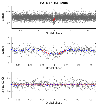
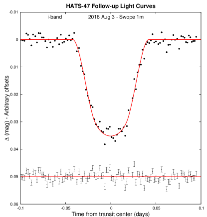
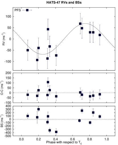
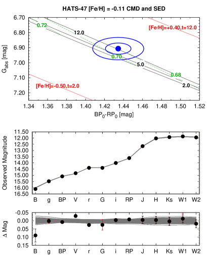
Figure 1: Observations used to confirm the transiting planet system HATS-47, excluding data from the NASA TESS mission which are shown in Figure 5. Top Left: Phase-folded unbinned HATSouth light curve. The top panel shows the full light curve, the middle panel shows the light curve zoomed-in on the transit, and the bottom panel shows the residuals from the best-fit model zoomed-in on the transit. The solid lines show the model fits to the light curves. The dark filled circles show the light curves binned in phase with a bin size of 0.002. (Caption continued on next page.)

Figure 1: (Caption continued from previous page.) Top Right: Unbinned follow-up transit light curves corrected for instrumental trends fitted simultaneously with the transit model, which is overplotted. The dates, filters and instruments used are indicated. In this figure the residuals are shown below the light curve. In Figures 2, 3 and 4, the residuals are shown on the right-hand-side in the same order as the original light curves. The error bars represent the photon and background shot noise, plus the readout noise. Note that these uncertainties are scaled up in the fitting procedure to achieve a reduced $\chi^{2}$ of unity, but the uncertainties shown in the plot have not been scaled. Bottom Left: High-precision RVs phased with respect to the mid-transit time. The instruments used are labelled in the plot. The top panel shows the phased measurements together with the best-fit model. The center-of-mass velocity has been subtracted. The second panel shows the velocity $O\!-\!C$ residuals. The error bars include the estimated jitter. The third panel shows the bisector spans. Bottom Right: Color-magnitude diagram (CMD) and spectral energy distribution (SED). The top panel shows the absolute $G$ magnitude vs. the de-reddened $BP-RP$ color compared to theoretical isochrones (black lines) and stellar evolution tracks (green lines) from the PARSEC models interpolated at the best-estimate value for the metallicity of the host. The age of each isochrone is listed in black in Gyr, while the mass of each evolution track is listed in green in solar masses. The solid red lines show isochrones at higher and lower metallicities than the best-estimate value, with the metallicity and age in Gyr of each isochrone labelled on the plot. The filled blue circles show the measured reddening- and distance-corrected values from Gaia DR2, while the blue lines indicate the $1\sigma$ and $2\sigma$ confidence regions, including the estimated systematic errors in the photometry. The middle panel shows the SED as measured via broadband photometry through the listed filters. Here we plot the observed magnitudes without correcting for distance or extinction. Overplotted are 200 model SEDs randomly selected from the MCMC posterior distribution produced through the global analysis (gray lines). The model makes use of the predicted absolute magnitudes in each bandpass from the PARSEC isochrones, the distance to the system (constrained largely via Gaia DR2) and extinction (constrained from the SED with a prior coming from the mwdust 3D Galactic extinction model). The bottom panel shows the $O\!-\!C$ residuals from the best-fit model SED.

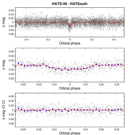
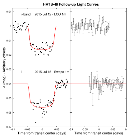
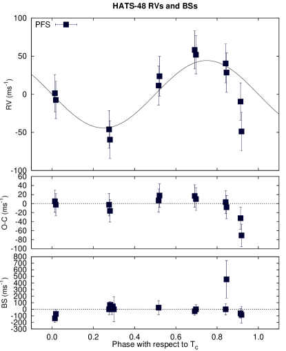
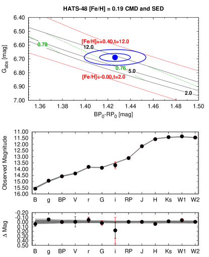
Figure 2: Same as Figure 1, here we show the observations of HATS-48A together with our best-fit model. The TESS light curve for this system is shown in Figure 6.

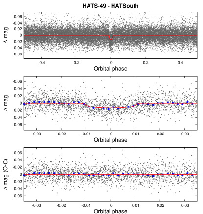
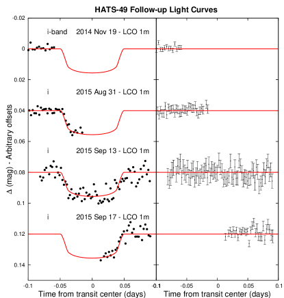
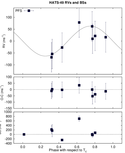
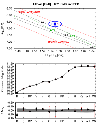
Figure 3: Same as Figure 1, here we show the observations of HATS-49 together with our best-fit model. The TESS light curve for this system is shown in Figure 7.

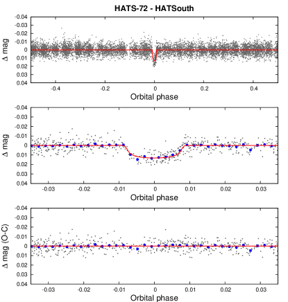
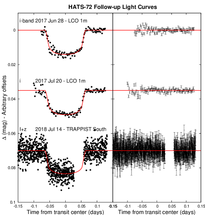
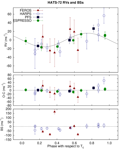
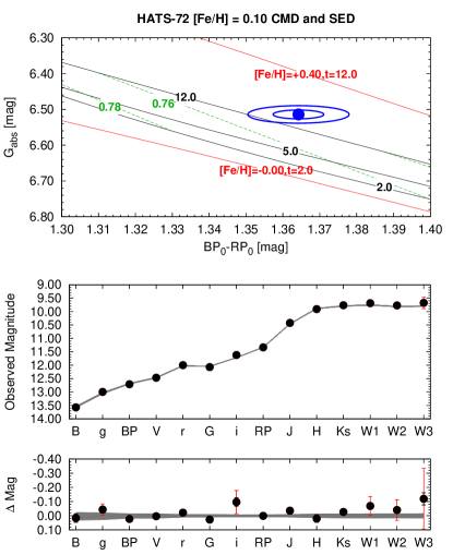
Figure 4: Same as Figure 1, here we show the observations of HATS-72 together with our best-fit model. The TESS light curve for this system is shown in Figure 8, while the WASP light curve is shown in Figure 9.

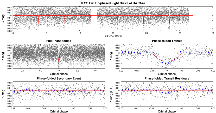
Figure 5: TESS short-cadence light curve for HATS-47. We show the full un-phased light curve as a function of time (top), the full phase-folded light curve (middle left), the phase-folded light curve zoomed-in on the planetary transit (middle right), the phase-folded light curve zoomed-in on the secondary eclipse (bottom left), and the residuals from the best-fit model, phase-folded and zoomed-in on the planetary transit (bottom right). The solid line in each panel shows the model fit to the light curve. The dark filled circles show the light curve binned in phase with a bin size of 0.002. Other observations included in our analysis of this system are shown in Figure 1. The TESS light curve has been corrected for dilution from neighbors as part of the PDC process, but in this case, where two bright neighbors are blended with the target in the TESS images, the correction appears to have been somewhat overestimated. This leads to a slightly deeper apparent transit in the TESS PDC light curve compared to the model. The model, however, fits the HATSouth and Swope 1 m transit observations (Fig. 1), which were obtained at sufficiently high spatial resolution to resolve the neighbors.

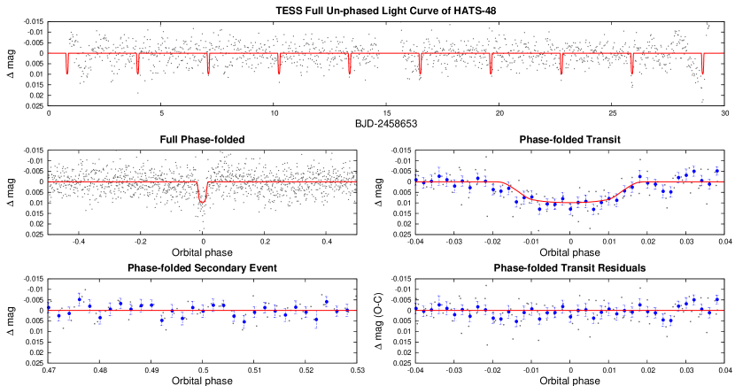
Figure 6: Similar to Figure 5, here we show the TESS long-cadence light curve for HATS-48A. The model lines account for the 30 min integrations. Other observations included in our analysis of this system are shown in Figure 2.

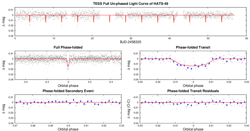
Figure 7: Similar to Figure 5, here we show the TESS long-cadence light curve for HATS-49. Other observations included in our analysis of this system are shown in Figure 3.

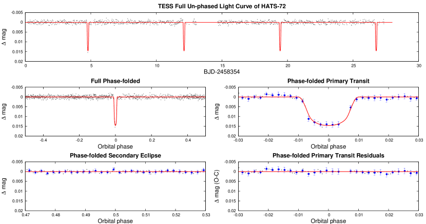
Figure 8: Similar to Figure 8, here we show the TESS long-cadence light curve for HATS-72. Other observations included in our analysis of this system are shown in Figures 4, and 9.

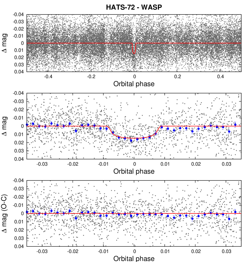
Figure 9: WASP light curve for HATS-72, displayed in a similar fashion to the HATSouth light curve shown in Figure 4 (see the caption in Figure 1). Other observations included in our analysis of this system are shown in Figure 4 and 8.

2.1.2 TESS

All four systems were observed by the NASA TESS mission as summarized in Table 1.

HATS-47 was observed in short-cadence mode through an approved TESS Guest-Investigator program (G011214; PI Bakos) to observe HATSouth transiting planet candidates with TESS. The short-cadence observations were reduced to light curves by the NASA Science Processing Operations Center (SPOC) Pipeline at NASA Ames Research Center (Jenkins et al., 2016, 2010). Two threshold crossing events were identified by this pipeline for this target, and the object was selected as a transiting planet candidate and assigned the TESS Object of Interest (TOI) identifier TOI 1073.01 by the TESS Science Office team after inspecting the data validation report produced by the SPOC pipeline. The target passed all of the data validation tests conducted by the pipeline, including no discernable difference between odd and even transits, no evidence for a weak secondary event, no evidence for stronger transits in a halo aperture compared to the optimal aperture used to extract the light curve, strong evidence that the target is not a false alarm due to correlated noise, and no evidence for variations in the difference image centroid. We obtained the SPOC PDC light curve (Stumpe et al., 2014; Smith et al., 2012) for HATS-47 from the Barbara A. Mikulski Archive for Space Telescopes (MAST).

HATS-47 is blended in the TESS images with two other comparably bright stars (the two neighbors are separated from HATS-47 by $33$″and $42$″). These neighbors are both well-resolved by HATSouth and the facility used for photometric follow-up observations (Section 2.3). A correction for dilution is applied in the PDC process, but may have been overestimated in this case leading to a slightly deeper transit seen in the TESS light curve (Fig. 5), compared to the other light curves (Fig. 1).

The TESS light curve of HATS-47 shows a clear quasi-sinusoidal out-of-transit variability with a period of $6.22158\pm 0.00011$ days and a semiamplitude of $5.79\pm 0.33$ mmag. The period is close to, but different from, the rotation period of $6.621581\pm 0.000078$ days estimated independently from the HATSouth light curve. The difference is presumably a result of starspot evolution and/or differential rotation. We take the average of these two measurements as our estimate for the photometric rotation period of the star ($6.42\pm 0.28$ days). We filtered the quasi-sinusoidal variation out of the TESS light curve of HATS-47 by fitting and subtracting a harmonic series to the data. The harmonic-filtered light curve is then used in the analysis (Section 3).

The other three targets were not included in the set of stars observed in short-cadence mode by the mission, so only $\sim 30$ min integrations from the Full Frame Images (FFIs) are available for these objects. Of these, HATS-72 was bright enough to have a light curve produced from the FFI observations by the TESS Quick Look Pipeline (QLP; Huang et al., 2018) at MIT. We made use of the detrended light curve for HATS-72 produced by this pipeline. For HATS-48A and HATS-49, which were not processed by SPOC, and were too faint to be processed through the QLP, we extracted light curves from the TESS FFIs using Lightkurve (Lightkurve Collaboration et al., 2018) and TESSCut (Brasseur et al., 2019), using a B-spline to remove trends on time-scales longer than the transits, and made use of these data in our analysis.

We note that HATS-47 and HATS-48A suffer significant blending from nearby stars in the low spatial-resolution TESS images, and the Sector 13 observations also have significant scattered light.

2.1.3 WASP

HATS-72 was observed by WASP-South over the period 2006 May to 2012 June, accumulating 24,200 data points. WASP-South is an array of 8 cameras combining 200-mm f/1.8 lenses with 2k$\times$2k CCDs and observing with a broad, 400–700 nm bandpass (Pollacco et al., 2006). It observed visible fields with a typical cadence of 15 min on each clear night. After identification of a candidate 7.33 d transit periodicity (see Collier Cameron et al. 2007), HATS-72 was placed on the WASP-South follow-up program in 2013 January. This led to nine RVs being observed with the Euler/CORALIE spectrograph (e.g. Triaud et al. 2013) over 2013–2018, and the observation in 2018 July of a transit with TRAPPIST-South (e.g. Gillon et al. 2013), using an I+z filter. The data were compatible with the transiting object being a planet, leading to a provisional designation as WASP-191b, but the low-amplitude meant that detection of orbital motion was not secure. Plans to acquire HARPS observations were then superseded by confirmation of the planet by the HATSouth team.

2.2 Spectroscopic Observations

The spectroscopic observations carried out to confirm and characterize the four transiting planet systems presented here are summarized in Table 3. The facilities are: WiFeS on the ANU 2.3 m (Dopita et al., 2007), PFS on the Magellan 6.5 m (Crane et al., 2006, 2008, 2010), FEROS on the MPG 2.2 m (Kaufer & Pasquini, 1998), HARPS on the ESO 3.6 m (Mayor et al., 2003), Coralie on the Euler 1.2 m (Queloz et al., 2001), and ESPRESSO on the VLT 8.2 m (Mégevand et al., 2014).

The WiFeS observations were obtained for HATS-47, HATS-48A and HATS-49, and were used for reconnaissance to rule out common false positives such as transiting very low mass stars, or eclipsing stellar binaries blended with a brighter giant star. The data were reduced following Bayliss et al. (2013). For each object we obtained spectra at resolving power $R\equiv\Delta\,\lambda\,/\,\lambda\approx 3000$ to estimate the effective temperature, $\log{g}$ and $\rm[Fe/H]$ of the star. Additional observations at $R\approx 7000$ were also obtained to search for any large amplitude radial velocity variations at the $\sim 4$ $\rm km\,s^{-1}$ level, which would indicate a stellar mass companion. All three systems were confirmed to be dwarf stars with RV variations below $4$ $\rm km\,s^{-1}$.

We obtained PFS observations of all four systems. For each system we obtained observations with an I₂ cell, and observations without the cell. The I₂-free observations were used to construct a template for measuring high-precision RVs from observations made with the cell following the method of Butler et al. (1996). The PFS RV observations were included in the modelling that we performed for all four systems (Section 3.1). Spectral line Bisector Span (BS) measurements and their uncertainties were measured as described by Jordán et al. (2014) and Brahm et al. (2017a).

We obtained FEROS observations for HATS-47, HATS-48A and HATS-72. These were reduced to wavelength-calibrated spectra, and high-precision RV and BS measurements using the CERES software package (Brahm et al., 2017a). Due to the faintness of HATS-47 and HATS-48A, we found that the scatter in the FEROS RV measurements for these two systems was too high to be useful in constraining the RV orbital variation of the host star. For the much brighter host HATS-72, however, we did incorporate FEROS data into the analysis.

The HARPS observations of HATS-72 were also reduced using CERES. The RVs were of high enough precision to be included in our analysis of this system. The HARPS observations reported here were obtained by the HATSouth team. We note that a single HARPS observation of this system was also independently obtained by the WASP team, but we do not include it in the analysis since it was gathered and reduced in a different manner from the observations obtained by the HATSouth team.

Coralie observations of HATS-72 were carried out by the WASP team independently of the other reported spectroscopic observations of this system, which were gathered by the HATSouth team. The observations constrain the orbital variation of the host star due to the planet to have a semi-amplitude less than $\sim 50$ $\rm m\,s^{-1}$. Additionally, no correlation is seen between the Coralie RV and BS measurements supporting a planetary interpretation of the observations.

Finally, we obtained ESPRESSO observations of HATS-72 after the HARPS, PFS and FEROS observations indicated a likely Super-Neptune mass for the planet. The observations were carried out through the queue service mode between 2019 May 11 and 2019 June 4. We obtained seven exposures of 1800 s, all made at an airmass below $1.2$, achieving a mean S/N per resolution element of $50$ at 550 nm. The ESPRESSO observations were reduced using version 1.3.2 of the ESPRESSO Data Analysis System (Cupani et al., 2018) in the ESO Reflex environment (Freudling et al., 2013), with the spectra cross-correlated against a K5 spectral mask to produce high-precision RVs. A more complete description of the observational setup and reduction procedure for the ESPRESSO observations obtained through our program will be provided in a forthcoming publication on the HATS-73 system (Bayliss et al. 2020, in preparation).

We also used the FEROS and I₂-free PFS observations to determine high-precision stellar atmospheric parameters for the host stars using the ZASPE package (Brahm et al., 2017b). The parameters that we measured include the effective temperature $T_{\rm eff\star}$, surface gravity $\log{g}$, metallicity $\rm[Fe/H]$, and $v\sin{i}$. The method involves cross-correlating the observed spectra against synthetic model spectra, and then obtaining error estimates for the parameters by performing a bootstrap analysis where the regions in the spectra that are most sensitive to changes in the atmospheric parameters are randomly adjusted based on the observed distribution of systematic mismatches between the observations and the best-matching model. This method allows for realistic parameter uncertainties that account, in a principled fashion, for systematic errors in the theoretical models. We performed this analysis on the PFS template spectra for HATS-47 and HATS-49, and on the FEROS spectra for HATS-48A and HATS-72. The resulting parameters are listed in Table 4.

The high-precision RV and BS measurements that were used in the analysis are given in Table 5 for all four systems.

Table 1: Summary of photometric observations

Instrument/Field	Date(s)	# Images	Cadence	Filter	Precision
			(sec)		(mmag)
HATS-47
HS-1/G747	2013 Mar–Oct	4231	287	$r$	15.9
HS-2/G747	2013 Sep–Oct	646	287	$r$	15.7
HS-3/G747	2013 Apr–Nov	9045	297	$r$	16.6
HS-4/G747	2013 Sep–Nov	1467	297	$r$	19.1
HS-5/G747	2013 Mar–Nov	6022	297	$r$	15.7
HS-6/G747	2013 Sep–Nov	1568	290	$r$	14.9
TESS/Sector 13	2019 Jun–Jul	1159	1798	$T$	3.3
Swope 1 m	2016 Aug 03	151	160	$i$	1.9
HATS-48A
HS-2/G778	2011 May–2012 Nov	2982	287	$r$	14.6
HS-4/G778	2011 Jul–2012 Nov	3726	298	$r$	13.5
HS-6/G778	2011 Apr–2012 Oct	2215	298	$r$	14.3
TESS/Sector 13	2019 Jun–Jul	1301	1798	$T$	5.2
LCO 1 m/SBIG	2015 Jul 12	61	201	$i$	2.3
Swope 1 m	2015 Jul 15	62	139	$i$	2.7
HATS-49
HS-2/G754	2012 Sep–Dec	3875	282	$r$	16.1
HS-4/G754	2012 Sep–2013 Jan	3197	292	$r$	17.7
HS-6/G754	2012 Sep–Dec	3002	285	$r$	17.0
HS-1/G755	2011 Jul–2012 Oct	5249	292	$r$	18.1
HS-3/G755	2011 Jul–2012 Oct	4828	287	$r$	19.0
HS-5/G755	2011 Jul–2012 Oct	6024	296	$r$	16.0
TESS/Sector 1	2018 Jul–Aug	1078	1798	$T$	4.8
TESS/Sector 2	2018 Aug–Sep	1219	1798	$T$	3.7
LCO 1 m/Sinistro	2014 Nov 19	34	288	$i$	1.5
LCO 1 m/Sinistro	2015 Aug 31	37	223	$i$	1.8
LCO 1 m/SBIG	2015 Sep 13	73	201	$i$	3.9
LCO 1 m/Sinistro	2015 Sep 17	30	223	$i$	3.0
HATS-72
HS-1/G537	2016 Jun–2016 Dec	4125	333	$r$	4.8
HS-3/G537	2016 Oct–2016 Dec	901	346	$r$	4.9
HS-5/G537	2016 Jun–2016 Dec	3354	365	$r$	4.8
WASP-South	2006 May–2011 Nov	24431	169	400–700 nm	21.8
TESS/Sector 3	2018 Aug–Sep	1036	1798	$T$	0.66
LCO 1 m/Sinistro	2017 Jun 28	107	163	$i$	1.3
LCO 1 m/Sinistro	2017 Jul 20	113	163	$i$	1.3
TRAPPIST-South	2018 Jul 14	1195	21	$I+z$	4.1

Table 2: Light curve data for HATS-47, HATS-48A, HATS-49, and HATS-72.

Object	BJD	Mag	$\sigma_{\rm Mag}$	Mag(orig)	Filter	Instrument
	(2,400,000$+$)
HATS-47	$2456492.53516$	$-0.01555$	$0.01509$	$\cdots$	$r$	HS
HATS-47	$2456570.99127$	$-0.01117$	$0.01041$	$\cdots$	$r$	HS
HATS-47	$2456555.30015$	$-0.05056$	$0.01484$	$\cdots$	$r$	HS
HATS-47	$2456551.37754$	$0.03031$	$0.01653$	$\cdots$	$r$	HS
HATS-47	$2456500.38125$	$-0.01951$	$0.01123$	$\cdots$	$r$	HS
HATS-47	$2456433.69366$	$-0.00988$	$0.01094$	$\cdots$	$r$	HS
HATS-47	$2456574.91475$	$-0.00262$	$0.00940$	$\cdots$	$r$	HS
HATS-47	$2456606.29725$	$-0.00778$	$0.01329$	$\cdots$	$r$	HS
HATS-47	$2456516.07293$	$-0.00670$	$0.01008$	$\cdots$	$r$	HS
HATS-47	$2456465.07680$	$-0.02574$	$0.01287$	$\cdots$	$r$	HS

Note. — This table is available in a machine-readable form in the online journal. A portion is shown here for guidance regarding its form and content.

Table 3: Summary of spectroscopy observations.

Instrument	UT Date(s)	# Spec.	Res.	S/N Range	$\gamma_{\rm RV}$	RV Precision
			$\Delta\lambda$/$\lambda$/1000		($\rm km\,s^{-1}$)	($\rm m\,s^{-1}$)
HATS-47
ANU 2.3 m/WiFeS	2015 Jun 1	1	3	28	$\cdots$	$\cdots$
ANU 2.3 m/WiFeS	2015 Jul 27–30	4	7	17–40	2.0	4000
Magellan 6.5 m/PFS+I2	2016 Mar–Aug	12	76	$\cdots$	$\cdots$	37
Magellan 6.5 m/PFS	2016 Mar 30	1	76	$\cdots$	$\cdots$	$\cdots$
MPG 2.2 m/FEROS	2016 Jul 1–26	5	48	14–33	3.179	55
HATS-48A
ANU 2.3 m/WiFeS	2014 Oct 4	1	3	49	$\cdots$	$\cdots$
ANU 2.3 m/WiFeS	2014 Oct 6–8	2	7	52–63	-22.5	4000
MPG 2.2 m/FEROS	2015 Jun–Oct	10	48	17–36	-22.457	75
Magellan 6.5 m/PFS+I2	2015 Jun–Oct	12	76	$\cdots$	$\cdots$	30
Magellan 6.5 m/PFS	2015 Jul 1	1	76	$\cdots$	$\cdots$	$\cdots$
HATS-49
ANU 2.3 m/WiFeS	2014 Oct 4–5	3	3	24–45	$\cdots$	$\cdots$
ANU 2.3 m/WiFeS	2014 Oct 5–7	2	7	24–48	8.1	4000
Magellan 6.5 m/PFS+I2	2015 Jan–2016 Jun	8	76	$\cdots$	$\cdots$	53
Magellan 6.5 m/PFS	2015 Jan 8	1	76	$\cdots$	$\cdots$	$\cdots$
HATS-72
ESO 3.6 m/HARPS	2017 Apr–2018 Aug	11	115	9–31	15.955	12.0
MPG 2.2 m/FEROS	2017 Jun–Aug	6	48	24–68	15.946	12.7
Euler 1.2 m/Coralie	2013 Jul–2018 Jul	9	60	42–46	$15.934$	$15$
Magellan 6.5 m/PFS+I2	2018 May–Aug	3	76	$\cdots$	$\cdots$	14.7
Magellan 6.5 m/PFS	2018 Jun 23	1	76	$\cdots$	$\cdots$	$\cdots$
VLT 8.2 m/ESPRESSO	2019 May–Jun	7	140	50	15.997	10.5

2.3 Photometric follow-up observations

Follow-up higher-precision ground-based photometric transit observations were obtained for all four systems, as summarized in Table 1. The facilities used for this purpose are: the Swope 1 m telescope at Las Campanas Observatory in Chile, 1 m telescopes from the Las Cumbres Observatory (LCOGT) network (Brown et al., 2013), and the 0.6 m TRAPPIST-South telescope at La Silla Observatory (Gillon et al., 2013). The follow-up observations using the Swope 1 m and the LCOGT 1 m network were performed by the HATSouth team, while the TRAPPIST-South observations of HATS-72 were performed by the WASP team. The exposure time for the TRAPPIST-South observations was 10 s, though with read-out, the median cadence was 21 s as listed in Table 1.

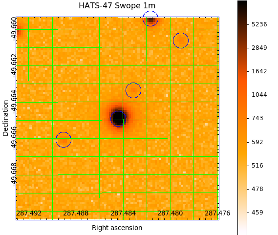
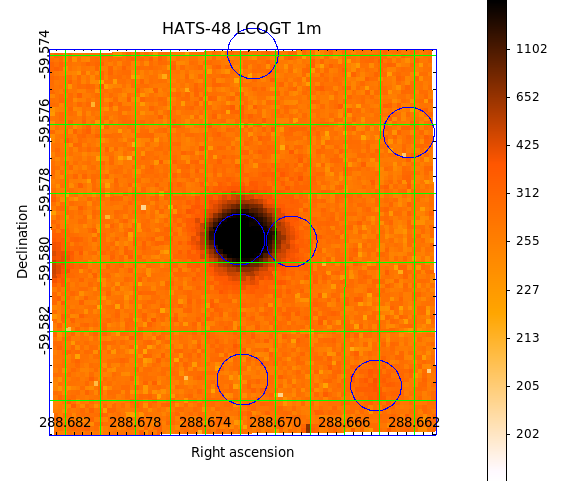
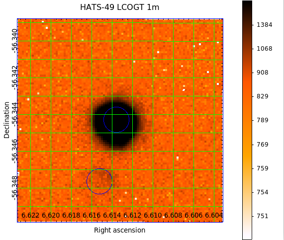
Figure 11: Snapshot $40\arcsec\times 40\arcsec$ images of HATS-47, HATS-48A, HATS-49 and HATS-72 selected from the ground-based time-series photometric follow-up observations obtained for each object. Each image is centered on the transiting planet host star. The blue circles indicate the positions of sources in the Gaia DR2 catalog, which is based on higher spatial resolution and deeper observations than the images shown here. The radius of each circle is equal to the approximate HWHM of the image PSF. Note that the LCOGT 1 m observations were carried out with defocusing to improve the photometric precision, while the Swope 1 m observations were carried out in-focus with the resolution limited by atmospheric seeing. The color scale indicates the number of counts (in ADU) in each calibrated image pixel, and is shown on an inverted logarithmic scale. All known neighbors are resolved in the ground-based photometric follow-up observations carried out for each system.

Figure 11 shows example $40\arcsec\times 40\arcsec$ images, centered on each target, selected from our photometric follow-up observations. In each case we overlay sources from the Gaia DR2 catalog, which is based on higher spatial resolution and deeper imaging than the photometric follow-up observations themselves. For all four objects all known neighbors have been resolved by the ground-based photometric follow-up observations.

Observations with the Swope 1 m and the reduction of the data to light curves were performed as described by Penev et al. (2013). The LCOGT 1 m observations were carried out in a similar manner to that described by Hartman et al. (2015), but were reduced using the methods applied by Penev et al. (2013) to data from the Faulkes Telescope South (FTS) 2 m, with some updates for automation to be described by Espinoza et al. (2020; in preparation). The TRAPPIST-South observations were carried out and reduced as described in Gillon et al. (2013).

The time-series photometry data are available in Table 2, and are plotted Figures 1, 2, 3, and 4.

2.4 Search for Resolved Stellar Companions

For HATS-47 and HATS-48A, the highest spatial resolution optical imaging available is from the Gaia mission (Gaia Collaboration et al., 2018). Gaia DR2 is sensitive to neighbors with $G\lesssim 20$ mag down to a limiting resolution of $\sim 1\arcsec$ (e.g., Ziegler et al., 2018).

There is a faint neighboring source to HATS-47 listed in the Gaia DR2 catalog at a projected separation of $6\farcs 4$ with $\Delta G=5.8$ mag. This object is fully resolved by the Swope 1 m photometric follow-up observations for which the seeing-limited resolution ranged between $1\farcs 4$ and $2\farcs 5$ FWHM. These observations show that the neighbor is not responsible for the transits, nor does it impact the transit depths measured in the follow-up observations. Based on the Gaia DR2 parallax measurements ($0.3\pm 1.3$ mas, compared to $3.298\pm 0.042$ mas for HATS-47), the neighboring source is in the background of HATS-47 and is not physically associated with it.

Similarly, there is a faint neighbor to HATS-48A in the Gaia DR2 catalog at a projected separation of $5\farcs 4$ and with $\Delta G=5.4$ mag. The neighbor has a parallax of $3.64\pm 0.44$ mas compared to $3.765\pm 0.024$ mas for HATS-48A, and a proper motion of $\mu_{\rm R.A.}=2.95\pm 0.47$ $\rm mas\,yr^{-1}$ and $\mu_{\rm Dec.}=5.20\pm 0.45$ $\rm mas\,yr^{-1}$, compared to $3.125\pm 0.031$ $\rm mas\,yr^{-1}$ and $6.146\pm 0.029$ $\rm mas\,yr^{-1}$ for HATS-48A. If we assume that this source is a physical binary companion to HATS-48A, and that it is a single star, then adopting the age, mass and metallicity for HATS-48A determined in Section 3.1 and listed in Table 6, and using the PARSEC stellar evolution models (Marigo et al., 2017), we find that $\Delta G=5.442\pm 0.004$ mag implies a mass of $0.224\pm 0.001$ $M_{\sun}$ for the companion. In that case the predicted $BP$ and $RP$ magnitude differences between the companion and HATS-48A are $\Delta BP=6.74$ mag and $\Delta RP=4.88$ mag, which are comparable to the observed differences of $\Delta BP=6.11\pm 0.12$ mag and $\Delta RP=4.80\pm 0.02$ mag. Note that theoretical isochrones are known to have errors in matching the optical photometry of late M dwarf stars, particularly in blue filters, so although the observed magnitude differences are off by more than the formal uncertainties, the results are close enough for us to conclude that the faint neighbor is most likely a bound physical companion to HATS-48A. Given the distance measured to HATS-48A, the neighbor is currently at a projected physical separation of $\sim$1,400 au from HATS-48A.

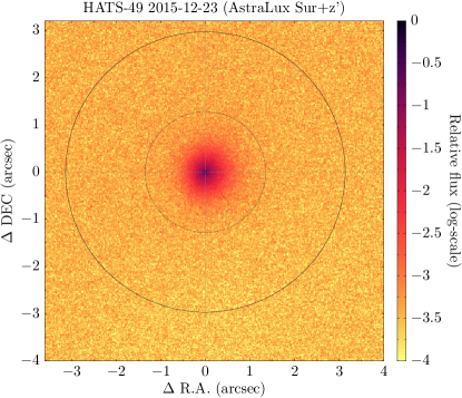
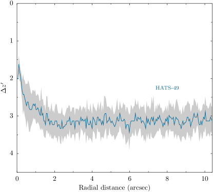
Figure 12: (left) High-resolution image of HATS-49 obtained with AstraLux Sur on the NTT through the $z^{\prime}$ filter. No neighboring sources are detected. (right) 5$\sigma$ upper limit on the magnitude contrast of any resolved neighbor to HATS-49 based on the Astralux Sur image. The gray band shows the variation in the limit with position angle.

We obtained high-angular resolution imaging of HATS-49 using the Astralux Sur imager (Hippler et al., 2009) on the New Technology Telescope (NTT). Observations were carried out in $z^{\prime}$-band on the night of 2015 December 23, and were reduced as in Espinoza et al. (2016). No neighbor was detected, and we place limits of $\Delta z^{\prime}>1.8\pm 0.2$ mag on neighbors down to $0\farcs 138$, and $\Delta z^{\prime}>3.1\pm 0.4$ mag at $\sim 1\farcs 5$. The image and contrast curve are shown in Figure 12. We also note that there is no neighbor within 10″ of HATS-49 listed in Gaia DR2.

High-angular resolution imaging of HATS-72 was reported by Ziegler et al. (2019) who carried out speckle imaging with SOAR to search for resolved stellar companions to 542 TESS planet candidate hosts. They report that no companion to HATS-72 was detected, and place magnitude contrast limits of $\Delta m>2.11$ mag and $\Delta m>3.60$ mag at separations of $0\farcs 15$ and 1″, respectively. We also note that there is no neighbor within 10″ of HATS-72 listed in Gaia DR2.

3 Analysis

3.1 Transiting Planet Modelling

We analyzed the photometric, spectroscopic and astrometric observations of each system to determine the stellar and planetary parameters following the methods described by Hartman et al. (2019), with modifications as summarized most recently by Bakos et al. (2018).

We perform a global fit to the light curves, RV curves, spectroscopically measured stellar atmospheric parameters, catalog broad-band photometry, and astrometric parallax from Gaia DR2. The fit is carried out using a modified version of the lfit program which is included in the fitsh software package (Pál, 2012). The light curves are modelled using the Mandel & Agol (2002) semi-analytic transit model with quadratic limb-darkening. The limb darkening coefficients are allowed to vary in the fit, using the tabulations from Claret et al. (2012, 2013) and Claret (2018) to place Gaussian prior constraints on their values, assuming a prior uncertainty of $0.2$ for each coefficient. The RV curves are modelled using the appropriate relations for Keplerian orbits.

We include in the model several parameters for the physical and observed properties of the host star, including the effective photospheric temperature, the metallicity, the distance modulus, and the $V$-band extinction $A_{V}$. These parameters are, in turn, constrained by the observed spectroscopic stellar atmospheric parameters (as measured in Section 2.2), the catalog photometry, and the parallax. Together with the parameters used to describe the transit and RV observations, these parameters are sufficient to determine the bulk physical properties of the stars and their transiting planets. We fit the data using two different methods for relating the stellar mass to the stellar radius, metallicity and luminosity: (1) an empirical method which uses the stellar bulk density measured from the transit and RV observations to determine the stellar mass from the stellar radius, which is itself inferred from the effective temperature and luminosity (this method is similar to that of, e.g., Stassun et al., 2017), and (2) using the PARSEC theoretical stellar evolution models (Marigo et al., 2017) to impose an additional constraint on the stellar relations that is typically tighter than the observed constraint on the stellar bulk density.

In each case, we model the data assuming the orbital eccentricity is zero, and we separately try allowing the eccentricity to be a free parameter.

A Differential Evolution Markov Chain Monte Carlo (DEMCMC) method is used to explore the parameter space and estimate the uncertainties based on the posterior parameter distribution. See Hartman et al. (2019) for a full list of the parameters that we vary, and their assumed priors.

We include in the fit the optical broad-band photometry from Gaia DR2 and APASS, NIR photometry from 2MASS, and IR photometry from WISE. For WISE we exclude the W4 band for all systems as none of the objects were detected in that bandpass, while for HATS-47, HATS-48A, and HATS-49 we also exclude the W3 band as the photometric uncertainty exceeds 0.1 mag in this bandpass for these three objects. These observations, together with the stellar atmospheric parameters, the parallax, and the reddening, constrain the luminosity of the star. To model the reddening, we assume a $R_{V}=3.1$ Cardelli et al. (1989) dust law parameterized by $A_{V}$, and use the mwdust 3D Galactic extinction model (Bovy et al., 2016) to place a prior constraint on its value.

We find that for all four transiting planet systems the orbits are consistent with being circular when the eccentricities are varied, and that the stellar parameters are more robustly constrained when imposing the theoretical stellar evolution model constraints. We therefore choose to adopt the parameters that stem from fixing the orbit to be circular, and imposing the stellar evolution models as a constraint on the stellar physical parameters.

The best-fit models are compared to the various observational data for the four transiting planet systems in Figures 1–9. The adopted stellar parameters derived from the analysis are listed in Table 6, while the adopted planetary parameters are listed in Table 7. We also list in Table 7 the 95% confidence upper limit on the eccentricity that comes from allowing the eccentricity to vary in the fit.

3.2 Stellar Blend Modelling

We also performed a blend modelling of each system following Hartman et al. (2019), where we attempt to fit all of the observations (except the RV data) using various combinations of stars, with parameters constrained by the PARSEC models. We find that for all four objects a model consisting of a single star with a transiting planet provides a better fit (a greater likelihood and a lower $\chi^{2}$) to the light curves, spectroscopic stellar atmospheric parameters, broad-band catalog photometry, and astrometric parallax measurements than the best-fit blended stellar eclipsing binary models. The blended stellar eclipsing binary models involve more free parameters than the transiting planet model, and thus can be rejected on the grounds that they are both poorer-fitting and more complicated models. Moreover, the fact that Keplerian orbital variations consistent with transiting planets are observed for all four objects, and that large spectral line bisector span variations are not observed is further evidence in favor of the transiting planet interpretation of the observations.

We also attempted to fit the systems as unresolved stellar binaries with a planet transiting the brighter stellar component. We find that for HATS-47 and HATS-48A there is no significant improvement in $\chi^{2}$ when adding an unresolved stellar binary companion compared to the model of a single star with a transiting planet. For HATS-49 and HATS-72 adding an unresolved companion does improve the fit, with $\Delta\chi^{2}=-17.4$ for HATS-49, and $\Delta\chi^{2}=-39.8$ for HATS-72. At face value this may be taken as evidence for an unresolved stellar companion to both of these objects. For HATS-49 this modelling yields a mass of $0.245\pm 0.039$ $M_{\sun}$ for the unresolved stellar companion, while for HATS-72 we find $0.317\pm 0.025$ $M_{\sun}$. However, as there is no other independent evidence for a stellar companion (such as a long-term trend in the RVs) for either of these objects, and as some low-mass stars (including late K dwarfs) have been observed to have larger radii than predicted by theoretical isochrones (e.g., Torres, 2013, in this case invoking an additional star would appear to reconcile the observations to the model leading to a better fit, but an erroneous conclusion), we do not consider this to be a clear detection of a stellar companion for either HATS-49 or HATS-72. Instead we present in Table 6 the 95% confidence upper limits on the mass of an unresolved companion for all four objects. High angular resolution imaging, long-term RV observations, and/or Gaia astrometry could potentially detect the companions if they are present.

4 Discussion

We have presented the discovery of four transiting giant planets on close-in orbits around K dwarf stars. Three of the planets presented in this paper, HATS-47b, HATS-48Ab, and HATS-49b, are comparable in mass to Saturn. The masses are $0.369_{-0.021}^{+0.031}$ $M_{\rm J}$, $0.243_{-0.030}^{+0.022}$ $M_{\rm J}$, and $0.353_{-0.027}^{+0.038}$ $M_{\rm J}$, respectively. Despite their relatively short orbital periods of $3.9228$ days, $3.1317$ days, and $4.1480$ days, all three of these planets can be considered warm giants with predicted equilibrium temperatures of $852.9\pm 4.7$ K, $954.6\pm 4.8$ K, and $834.8\pm 3.6$ K (estimated assuming zero-albedo and full redistribution of heat; note that the small uncertainties listed here do not account for the possibility that these assumptions are wrong, or for systematic errors in the stellar evolution models). This is due to the planets orbiting cool K dwarf stars with respective masses of $0.674_{-0.012}^{+0.016}$ $M_{\sun}$, $0.7279\pm 0.0066$ $M_{\sun}$, and $0.7133\pm 0.0075$ $M_{\sun}$. The fourth planet, HATS-72b, is a Super-Neptune with a mass of $0.1254\pm 0.0039$ $M_{\rm J}$, and with a somewhat longer orbital period of $7.3279$ days. This planet also orbits a cool K dwarf star of mass $0.7311\pm 0.0028$ $M_{\sun}$, and has a modest predicted equilibrium temperature of $739.3\pm 1.6$ K.

Figures 13 and 14 compare the planet masses, planet radii, average incident fluxes, host star masses, and orbital semi-major axes of the four systems presented in this paper to other published giant transiting planets listed in the NASA Exoplanet Archive with $R_{p}>0.5$ $R_{\rm J}$ and with measured masses. We show the comparison to all planets that satisfy these restrictions, and to only those found around stars with $M<0.8$ $M_{\sun}$. The four objects presented here are consistent with established trends. Notably, all four objects have relatively small radii ($1.117\pm 0.014$ $R_{\rm J}$, $0.800\pm 0.015$ $R_{\rm J}$, $0.765\pm 0.013$ $R_{\rm J}$, and $0.7224\pm 0.0032$ $R_{\rm J}$, for HATS-47b–HATS-49b, and HATS-72b, respectively) as expected for their low masses and modest irradiation. This makes the planets potentially useful objects for comparing to theoretical models of giant planet structure to infer their bulk heavy element contents. The planets all have semi-major axes that are beyond the empirical minimum semi-major axis as a function of planet mass, as seen in the top-right panel of Figure 14. As seen in the bottom panels of Figures 13 and 14, the four planets discovered here are among a still fairly small sample of giant planets known around stars with $M<0.8$ $M_{\sun}$, and may be useful in that sense for studying the formation and properties of close-in giant planets around low mass stars.

HATS-47b and HATS-72b are also notable for their relatively deep transits. With a transit depth of 3%, (e.g., Fig. 1), HATS-47 is among the deepest known transiting planet systems. Only HATS-71b (Bakos et al., 2018), WTS-2b (Birkby et al., 2014), HATS-6b (Hartman et al., 2015), and Kepler-45b (Johnson et al., 2012) are known to have deeper transits. Nearly as deep are the transits of WASP-80b (Triaud et al., 2013), POTS-1b (Koppenhoefer et al., 2013), Qatar-2b (Bryan et al., 2012), and CoRoT-2b (Alonso et al., 2008). The large transit depth makes HATS-47b a potentially attractive target for follow-up observations, such as transmission spectroscopy, for which the signal strength scales with the transit depth. With a transit depth of 1.1% (e.g., Fig. 4), HATS-72b stands out as having the deepest transits among all known planets with $M_{p}<0.15$ $M_{\rm J}$, making it a valuable target as well for transmission spectroscopy, in this case to study the atmosphere of a Super-Neptune. With an optical magnitude of $V=12.469\pm 0.010$ mag and NIR magnitude of $J=10.424\pm 0.023$ mag, HATS-72 is only slightly fainter than HAT-P-26 ($V=11.74$ mag, $J=10.08$ mag) which hosts a Neptune, and is significantly brighter than the super-Earth-hosting K2-18 in the visual band ($V=13.5$) and only somewhat fainter at near-infrared wavelenghts ($J=9.76$ mag). Both of these planets produce shallower transits than HATS-72b, and have had molecules detected in their atmospheres via transmission spectroscopy (Tsiaras et al., 2019; Benneke et al., 2019; Wakeford et al., 2017).

HATS-72 and HATS-73 (Bayliss et al. 2020, in preparation) are the first two systems confirmed by our team using ESPRESSO. This facility has been vital in confirming a relatively low amplitude signal ($16.15\pm 0.51$ $\rm m\,s^{-1}$) around cool stars. The benefits of this facility are derived not only from the increased mirror size and spectrograph efficiency, but also from the redder wavelength coverage of ESPRESSO which is important as we push to cooler host stars.

The combination of transit survey and follow-up data from three separate projects (HATSouth, TESS and WASP) also demonstrates the benefits of collaboration between surveys going forward. This is particularly so for HATS-72b, which was independently detected by all three surveys. As TESS continues its survey of the sky for transiting planets around bright stars, most if not all systems that have previously been identified by ground-based surveys will be observed by TESS. Through the coordination of TFOP, redundant follow-up observations can be avoided for transiting planet systems that have already been identified and confirmed by ground-based surveys, but have not yet been published. Coordination by TFOP also ensures greater efficiency in the analysis and publication of transiting planets such as these, by enabling data independently collected by different groups to be combined and analyzed in a single work.

Finally, this paper also illustrates a useful science contribution of ground-based transit surveys that is complimentary to the primary TESS mission. Neither of the planets HATS-48Ab or HATS-49b were identified as transiting planet candidates by the TESS team. Both of these objects are relatively faint with $V=14.35\pm 0.11$ mag for HATS-48A and $V=14.998\pm 0.040$ mag for HATS-49, and are not among the targets that have been searched for transits by the TESS team, which is focused on searching bright stars around which small planets may be detectable. However, to discover transiting giant planets around low-mass stars it is necessary to search a large number of M dwarfs and late K dwarfs, and thus to consider stars that are faint in the optical band-passes. Ground-based surveys like HATSouth, combined with independent analyses of the TESS FFIs being released to the public, are providing valuable contributions addressing this science topic.

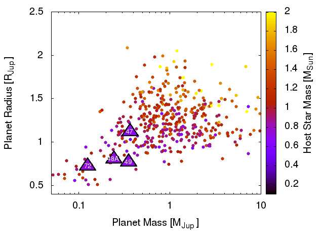
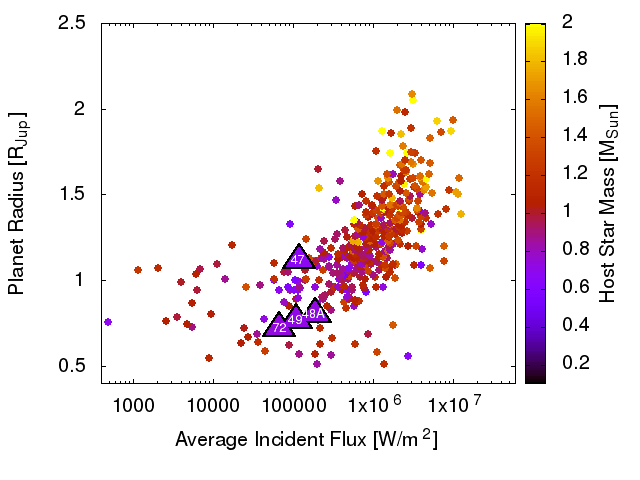
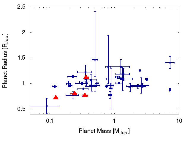
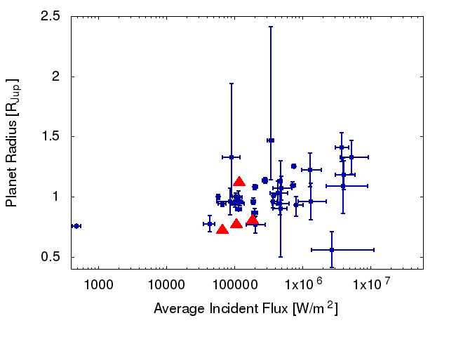
Figure 13: Top: Giant transiting planet radius vs. planet mass (left) and average incident flux (right). The four transiting planets presented in this paper are shown with large filled triangles, and are labelled by the HATS object number. The smaller filled circles show confirmed transiting giant planets with $R_{p}>0.5$ $R_{\rm J}$ and with measured masses (excluding objects where only an upper limit on the mass has been set) taken from the NASA Exoplanet Archive accessed 2019 Sep. 9. The color of each symbol indicates the mass of the transiting planet host star. Bottom: Similar to the top, but here we show only transiting planets around stars with $M<0.8$ $M_{\sun}$, we do not show the host star mass, but we do include the $1\sigma$ errorbars. The four planets presented in this paper are shown by the red filled triangles. Errorbars on the planet radius and incident flux are smaller than the symbols for these four planets.

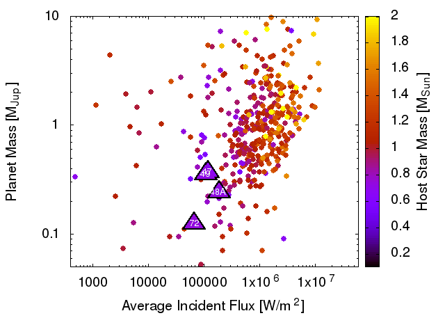
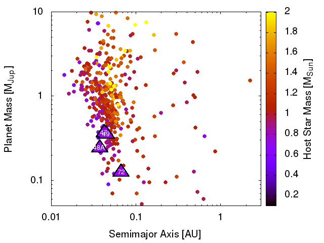
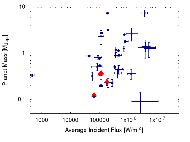
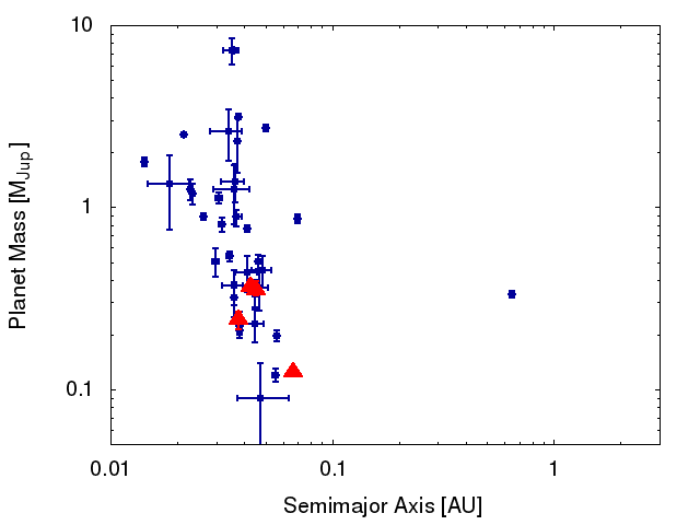
Figure 14: Similar to Fig. 13, here we show giant transiting planet mass vs. average incident flux (left) and semimajor axis (right). HATS-47b and HATS-49b overlap on these plots. As in Fig. 13, only planets with $R_{p}>0.5$ $R_{\rm J}$, and with measured masses are shown.

Table 4: Astrometric, Spectroscopic and Photometric parameters for HATS-47, HATS-48A, HATS-49 and HATS-72

	HATS-47	HATS-48A	HATS-49	HATS-72
Parameter	Value	Value	Value	Value	Source
Astrometric properties and cross-identifications
2MASS-ID	19095625-4939538	19144126-5934458	00262717-5620395	22360631-1659597
TIC-ID	158297421	201642601	281541545	188570092
TOI-ID	1073.01	$\cdots$	$\cdots$	294.01
GAIA DR2-ID	6658373007402886400	6638412919991750912	4919770108539385472	2594869603582993792
R.A. (J2000)	$19^{\mathrm{h}}09^{\mathrm{m}}56.2504{\mathrm{s}}$	$19^{\mathrm{h}}14^{\mathrm{m}}41.2748{\mathrm{s}}$	$00^{\mathrm{h}}26^{\mathrm{m}}27.1829{\mathrm{s}}$	$22^{\mathrm{h}}36^{\mathrm{m}}06.3190{\mathrm{s}}$	GAIA DR2
Dec. (J2000)	$-49{\arcdeg}39{\arcmin}53.868{\arcsec}$	$-59{\arcdeg}34{\arcmin}45.7571{\arcsec}$	$-56{\arcdeg}20{\arcmin}39.5352{\arcsec}$	$-16{\arcdeg}59{\arcmin}59.7882{\arcsec}$	GAIA DR2
$\mu_{\rm R.A.}$ ($\rm mas\,yr^{-1}$)	$3.827\pm 0.058$	$3.125\pm 0.031$	$42.581\pm 0.035$	$-108.621\pm 0.090$	GAIA DR2
$\mu_{\rm Dec.}$ ($\rm mas\,yr^{-1}$)	$4.878\pm 0.038$	$6.146\pm 0.029$	$8.264\pm 0.030$	$-84.412\pm 0.078$	GAIA DR2
parallax (mas)	$3.298\pm 0.042$	$3.765\pm 0.024$	$3.054\pm 0.022$	$7.809\pm 0.037$	GAIA DR2
Spectroscopic properties
$T_{\rm eff\star}$ (K)	$4479\pm 51$	$4190\pm 100$	$4354\pm 70$	$4612\pm 76$	ZASPE
$\rm[Fe/H]$	$-0.140\pm 0.066$	$0.00\pm 0.10$	$0.080\pm 0.084$	$-0.040\pm 0.050$	ZASPE
$v\sin{i}$ ($\rm km\,s^{-1}$)	$2.47\pm 0.70$	$0.73\pm 0.55$	$0.50\pm 0.78$	$0.8\pm 1.3$	ZASPE
$v_{\rm mac}$ ($\rm km\,s^{-1}$)	$1.994\pm 0.077$	$1.55\pm 0.15$	$1.80\pm 0.11$	$2.20\pm 0.12$	Assumed
$v_{\rm mic}$ ($\rm km\,s^{-1}$)	$0.326\pm 0.048$	$0.000\pm 0.085$	$0.197\pm 0.076$	$0.443\pm 0.061$	Assumed
$\gamma_{\rm RV}$ ($\rm m\,s^{-1}$)	$3197\pm 31$	$-22460\pm 21$	$8100\pm 1500$	$15954.8\pm 1.8$	FEROS or WiFeS
Photometric properties
$P_{\rm rot}$ (d)	$6.42\pm 0.28$	$\cdots$	$\cdots$	$48.725\pm 0.015$	HATSouth
$G$ (mag)	$14.39980\pm 0.00040$	$13.89510\pm 0.00020$	$14.54490\pm 0.00030$	$12.07250\pm 0.00030$	GAIA DR2
$BP$ (mag)	$15.0858\pm 0.0021$	$14.5801\pm 0.0016$	$15.2886\pm 0.0022$	$12.7084\pm 0.0018$	GAIA DR2
$RP$ (mag)	$13.61140\pm 0.00090$	$13.11260\pm 0.00090$	$13.7214\pm 0.0013$	$11.3341\pm 0.0010$	GAIA DR2
$B$ (mag)	$16.101\pm 0.040$	$15.577\pm 0.050$	$16.378\pm 0.040$	$13.572\pm 0.030$	APASS
$V$ (mag)	$14.829\pm 0.010$	$14.35\pm 0.11$	$14.998\pm 0.040$	$12.469\pm 0.010$	APASS
$g$ (mag)	$15.480\pm 0.010$	$14.935\pm 0.030$	$15.668\pm 0.040$	$12.995\pm 0.010$	APASS
$r$ (mag)	$14.398\pm 0.010$	$13.821\pm 0.050$	$14.496\pm 0.010$	$11.998\pm 0.010$	APASS
$i$ (mag)	$14.009\pm 0.010$	$13.69\pm 0.17$	$14.14\pm 0.12$	$11.622\pm 0.030$	APASS
$J$ (mag)	$12.653\pm 0.023$	$12.160\pm 0.024$	$12.692\pm 0.024$	$10.424\pm 0.023$	2MASS
$H$ (mag)	$12.026\pm 0.023$	$11.591\pm 0.026$	$12.105\pm 0.024$	$9.907\pm 0.026$	2MASS
$K_{s}$ (mag)	$11.926\pm 0.025$	$11.427\pm 0.021$	$11.938\pm 0.023$	$9.764\pm 0.021$	2MASS
$W1$ (mag)	$11.867\pm 0.023$	$11.364\pm 0.023$	$11.903\pm 0.023$	$9.687\pm 0.024$	WISE
$W2$ (mag)	$11.947\pm 0.024$	$11.458\pm 0.021$	$11.990\pm 0.022$	$9.772\pm 0.020$	WISE
$W3$ (mag)	$11.707\pm 0.192$	$11.433\pm 0.135$	$12.212\pm 0.256$	$9.675\pm 0.043$	WISE

Table 5: Relative radial velocities and bisector spans for HATS-47, HATS-48A, HATS-49 and HATS-72.

System	BJD	RV	$\sigma_{\rm RV}$	BS	$\sigma_{\rm BS}$	Phase	Instrument
	(2,450,000$+$)	($\rm m\,s^{-1}$)	($\rm m\,s^{-1}$)	($\rm m\,s^{-1}$)	($\rm m\,s^{-1}$)
HATS-47	$7472.87421$	$-73.25$	$9.58$	$-379.5$	$95.6$	$0.408$	PFS
HATS-47	$7474.88339$	$17.75$	$9.26$	$84.1$	$58.3$	$0.920$	PFS
HATS-47	$7477.86812$	$\cdots$	$\cdots$	$-38.4$	$48.8$	$0.681$	PFS
HATS-47	$7477.90415$	$68.00$	$12.60$	$\cdots$	$\cdots$	$0.690$	PFS
HATS-47	$7507.88072$	$-33.23$	$11.94$	$-331.8$	$71.1$	$0.332$	PFS
HATS-47	$7530.84061$	$-93.65$	$13.98$	$60.7$	$177.1$	$0.185$	PFS
HATS-47	$7534.82504$	$-40.07$	$8.01$	$304.7$	$67.2$	$0.200$	PFS
HATS-47	$7536.82554$	$47.53$	$9.89$	$262.1$	$71.0$	$0.710$	PFS
HATS-47	$7558.79646$	$43.22$	$10.65$	$89.5$	$133.0$	$0.311$	PFS
HATS-47	$7615.65549$	$29.50$	$8.55$	$-98.7$	$49.9$	$0.806$	PFS

Note. — This table is available in a machine-readable form in the online journal. A portion is shown here for guidance regarding its form and content.

Table 6: Adopted derived stellar parameters for HATS-47, HATS-48A, HATS-49 and HATS-72.

	HATS-47	HATS-48A	HATS-49	HATS-72
Parameter	Value	Value	Value	Value
$M_{\star}$ ($M_{\sun}$)	$0.674_{-0.012}^{+0.016}$	$0.7279\pm 0.0066$	$0.7133\pm 0.0075$	$0.7311\pm 0.0028$
$R_{\star}$ ($R_{\sun}$)	$0.6564\pm 0.0055$	$0.7152\pm 0.0038$	$0.6977\pm 0.0055$	$0.7214\pm 0.0021$
$\log{g_{\star}}$ (cgs)	$4.633\pm 0.011$	$4.5909\pm 0.0039$	$4.6036\pm 0.0077$	$4.5853\pm 0.0021$
$\rho_{\star}$ ($\rm g\,cm^{-3}$)	$3.360_{-0.099}^{+0.130}$	$2.804\pm 0.036$	$2.961\pm 0.073$	$2.743\pm 0.020$
$L_{\star}$ ($L_{\sun}$)	$0.1599\pm 0.0031$	$0.1955\pm 0.0042$	$0.1641\pm 0.0026$	$0.2193\pm 0.0021$
$T_{\rm eff\star}$ (K)	$4512\pm 19$	$4546_{-18}^{+23}$	$4405\pm 15$	$4656.1\pm 8.9$
$\rm[Fe/H]$	$-0.113\pm 0.035$	$0.186\pm 0.051$	$0.208\pm 0.053$	$0.099\pm 0.014$
Age (Gyr)	$8.1_{-4.3}^{+2.9}$	$11.97_{-0.61}^{+0.42}$	$10.5_{-2.0}^{+1.4}$	$12.17_{-0.45}^{+0.24}$
$A_{V}$ (mag)	$0.108\pm 0.032$	$0.112\pm 0.033$	$0.046\pm 0.014$	$0.0270\pm 0.0080$
Distance (pc)	$301.7\pm 1.9$0	$265.4\pm 1.7$	$324.6\pm 2.2$	$127.66\pm 0.52$
MB ($M_{\sun}$)	$<0.23$	$0.22$	$<0.31$	$<0.36$

Note. — The listed parameters are those determined through the joint differential evolution Markov Chain analysis described in Section 3.1. For all four systems the RV observations are consistent with a circular orbit, and we assume a fixed circular orbit in generating the parameters listed here. Systematic errors in the bolometric correction tables or stellar evolution models are not included, and may dominate the error budget for some of these parameters.

Table 7: Adopted orbital and planetary parameters for HATS-47b, HATS-48Ab, HATS-49b and HATS-72b

	HATS-47b	HATS-48Ab	HATS-49b	HATS-72b
Parameter	Value	Value	Value	Value
Light curve parameters
$P$ (days)	$3.9228038\pm 0.0000022$	$3.1316666\pm 0.0000037$	$4.1480467\pm 0.0000037$	$7.3279474\pm 0.0000016$
$T_{c}$ (${\rm BJD\_{}TDB}$)	$2457365.35804\pm 0.00029$	$2457100.55022\pm 0.00045$	$2457105.16480\pm 0.00054$	$2458087.647820\pm 0.000075$
$T_{14}$ (days)	$0.08343\pm 0.00089$	$0.09774\pm 0.00050$	$0.09775\pm 0.00095$	$0.12853\pm 0.00030$
$T_{12}=T_{34}$ (days)	$0.02313\pm 0.00067$	$0.01015\pm 0.00020$	$0.01184\pm 0.00036$	$0.012258\pm 0.000080$
$a/R_{\star}$	$13.98\pm 0.15$	$11.330\pm 0.049$	$13.91\pm 0.11$	$19.821\pm 0.048$
$\zeta/R_{\star}$	$31.93\pm 0.46$0	$22.825_{-0.098}^{+0.130}$0	$23.22\pm 0.31$0	$17.195\pm 0.049$0
$R_{p}/R_{\star}$	$0.1746\pm 0.0014$	$0.1148\pm 0.0020$	$0.1127\pm 0.0015$	$0.10290\pm 0.00034$
$b^{2}$	$0.508_{-0.014}^{+0.014}$	$0.0069_{-0.0046}^{+0.0080}$	$0.176_{-0.028}^{+0.022}$	$0.0233_{-0.0066}^{+0.0054}$
$b\equiv a\cos i/R_{\star}$	$0.7127_{-0.0096}^{+0.0096}$	$0.083_{-0.035}^{+0.039}$	$0.420_{-0.035}^{+0.025}$	$0.153_{-0.023}^{+0.017}$
$i$ (deg)	$87.080\pm 0.061$0	$89.58\pm 0.18$0	$88.27_{-0.11}^{+0.16}$0	$89.560_{-0.050}^{+0.070}$0
Dilution factors
HATSouth 1	$0.920\pm 0.037$	$0.998940\pm 0.000094$	$0.811\pm 0.049$	$0.868\pm 0.022$
HATSouth 2	$\cdots$	$\cdots$	$0.799\pm 0.049$	$\cdots$
TESS	$0.869\pm 0.012$	$0.597\pm 0.024$	$0.755\pm 0.069$	$0.97763\pm 0.00052$
WASP	$\cdots$	$\cdots$	$\cdots$	$0.984\pm 0.012$
Limb-darkening coefficients
$c_{1},r$	$0.49\pm 0.13$	$0.36\pm 0.14$	$0.67\pm 0.12$	$0.423_{-0.080}^{+0.061}$
$c_{2},r$	$0.28_{-0.12}^{+0.15}$	$0.32\pm 0.15$	$0.16\pm 0.17$	$0.508\pm 0.088$
$c_{1},i$	$0.53\pm 0.13$	$0.22\pm 0.11$	$0.34\pm 0.11$	$0.316\pm 0.059$
$c_{2},i$	$0.38_{-0.16}^{+0.12}$	$0.17\pm 0.16$	$0.06\pm 0.14$	$0.444\pm 0.097$
$c_{1},T$	$0.460\pm 0.100$	$0.41\pm 0.12$	$0.56\pm 0.17$	$0.503\pm 0.060$
$c_{2},T$	$0.41\pm 0.11$	$0.34\pm 0.14$	$0.24\pm 0.15$	$0.403\pm 0.084$
$c_{1},I+z$	$\cdots$	$\cdots$	$\cdots$	$0.262\pm 0.060$
$c_{2},I+z$	$\cdots$	$\cdots$	$\cdots$	$0.305\pm 0.078$
$c_{1},{\rm WASP}$	$\cdots$	$\cdots$	$\cdots$	$0.524\pm 0.077$
$c_{2},{\rm WASP}$	$\cdots$	$\cdots$	$\cdots$	$0.349\pm 0.074$
RV parameters
$K$ ($\rm m\,s^{-1}$)	$61.7\pm 4.3$00	$41.8\pm 4.4$00	$55.9\pm 5.5$00	$16.15\pm 0.51$00
$e$	$<0.088$	$<0.162$	$<0.071$	$<0.013$
RV jitter PFS ($\rm m\,s^{-1}$)	$40.4\pm 8.9$	$25.2\pm 6.2$	$57\pm 13$	$6.4\pm 1.7$
RV jitter ESPRESSO ($\rm m\,s^{-1}$)	$\cdots$	$\cdots$	$\cdots$	$8.25\pm 0.32$
RV jitter HARPS ($\rm m\,s^{-1}$)	$\cdots$	$\cdots$	$\cdots$	$1.13\pm 0.42$
RV jitter FEROS ($\rm m\,s^{-1}$)	$\cdots$	$\cdots$	$\cdots$	$18.7\pm 6.3$
Planetary parameters
$M_{p}$ ($M_{\rm J}$)	$0.369_{-0.021}^{+0.031}$	$0.243_{-0.030}^{+0.022}$	$0.353_{-0.027}^{+0.038}$	$0.1254\pm 0.0039$
$R_{p}$ ($R_{\rm J}$)	$1.117\pm 0.014$	$0.800\pm 0.015$	$0.765\pm 0.013$	$0.7224\pm 0.0032$
$C(M_{p},R_{p})$	$-0.00$	$0.16$	$0.31$	$0.30$
$\rho_{p}$ ($\rm g\,cm^{-3}$)	$0.331\pm 0.027$	$0.589\pm 0.067$	$0.986\pm 0.094$	$0.4110_{-0.0100}^{+0.0150}$
$\log g_{p}$ (cgs)	$2.866\pm 0.032$	$2.978_{-0.058}^{+0.036}$	$3.177\pm 0.040$	$2.774\pm 0.013$
$a$ (AU)	$0.04269_{-0.00025}^{+0.00033}$	$0.03769\pm 0.00011$	$0.04515\pm 0.00016$	$0.066517\pm 0.000085$
$T_{\rm eq}$ (K)	$852.9\pm 4.7$	$954.6\pm 4.8$	$834.8\pm 3.6$	$739.3\pm 1.6$
$\Theta$	$0.0418_{-0.0025}^{+0.0034}$	$0.0317_{-0.0041}^{+0.0027}$	$0.0585_{-0.0045}^{+0.0059}$	$0.03150\pm 0.00097$
$\log_{10}\langle F\rangle$ (cgs)	$8.0770\pm 0.0095$	$8.2725\pm 0.0086$	$8.0394\pm 0.0073$	$7.8292\pm 0.0038$

Note. — For all systems we adopt a model in which the orbit is assumed to be circular. See the discussion in Section 3.1.

References

- Alonso et al. (2008) Alonso, R., Auvergne, M., Baglin, A., et al. 2008, A&A, 482, L21
- Astropy Collaboration et al. (2013) Astropy Collaboration, Robitaille, T. P., Tollerud, E. J., et al. 2013, A&A, 558, A33
- Bakos et al. (2004) Bakos, G., Noyes, R. W., Kovács, G., et al. 2004, PASP, 116, 266
- Bakos et al. (2010) Bakos, G. Á., Torres, G., Pál, A., et al. 2010, ApJ, 710, 1724
- Bakos et al. (2013) Bakos, G. Á., Csubry, Z., Penev, K., et al. 2013, PASP, 125, 154
- Bakos et al. (2018) Bakos, G. Á., Bayliss, D., Bento, J., et al. 2018, arXiv e-prints, arXiv:1812.09406
- Bayliss et al. (2013) Bayliss, D., Zhou, G., Penev, K., et al. 2013, AJ, 146, 113
- Benneke et al. (2019) Benneke, B., Wong, I., Piaulet, C., et al. 2019, ApJ, 887, L14
- Bertin & Arnouts (1996) Bertin, E., & Arnouts, S. 1996, A&AS, 117, 393
- Birkby et al. (2014) Birkby, J. L., Cappetta, M., Cruz, P., et al. 2014, MNRAS, 440, 1470
- Borucki et al. (2010) Borucki, W. J., Koch, D., Basri, G., et al. 2010, Science, 327, 977
- Bovy et al. (2016) Bovy, J., Rix, H.-W., Green, G. M., Schlafly, E. F., & Finkbeiner, D. P. 2016, ApJ, 818, 130
- Brahm et al. (2017a) Brahm, R., Jordán, A., & Espinoza, N. 2017a, Publications of the Astronomical Society of the Pacific, 129, 034002
- Brahm et al. (2017b) Brahm, R., Jordán, A., Hartman, J., & Bakos, G. 2017b, MNRAS, 467, 971
- Brasseur et al. (2019) Brasseur, C. E., Phillip, C., Fleming, S. W., Mullally, S. E., & White, R. L. 2019, Astrocut: Tools for creating cutouts of TESS images, , , ascl:1905.007
- Brown et al. (2013) Brown, T. M., Baliber, N., Bianco, F. B., et al. 2013, PASP, 125, 1031
- Bryan et al. (2012) Bryan, M. L., Alsubai, K. A., Latham, D. W., et al. 2012, ApJ, 750, 84
- Butler et al. (1996) Butler, R. P., Marcy, G. W., Williams, E., et al. 1996, PASP, 108, 500
- Cardelli et al. (1989) Cardelli, J. A., Clayton, G. C., & Mathis, J. S. 1989, ApJ, 345, 245
- Charbonneau et al. (2000) Charbonneau, D., Brown, T. M., Latham, D. W., & Mayor, M. 2000, ApJ, 529, L45
- Claret (2018) Claret, A. 2018, A&A, 618, A20
- Claret et al. (2012) Claret, A., Hauschildt, P. H., & Witte, S. 2012, A&A, 546, A14
- Claret et al. (2013) —. 2013, A&A, 552, A16
- Collier Cameron et al. (2007) Collier Cameron, A., Wilson, D. M., West, R. G., et al. 2007, MNRAS, 380, 1230
- Collins et al. (2018) Collins, K., Quinn, S. N., Latham, D. W., et al. 2018, in American Astronomical Society Meeting Abstracts, Vol. 231, American Astronomical Society Meeting Abstracts #231, 439.08
- Crane et al. (2006) Crane, J. D., Shectman, S. A., & Butler, R. P. 2006, in Society of Photo-Optical Instrumentation Engineers (SPIE) Conference Series, Vol. 6269, Society of Photo-Optical Instrumentation Engineers (SPIE) Conference Series, 626931
- Crane et al. (2010) Crane, J. D., Shectman, S. A., Butler, R. P., et al. 2010, in Society of Photo-Optical Instrumentation Engineers (SPIE) Conference Series, Vol. 7735, Society of Photo-Optical Instrumentation Engineers (SPIE) Conference Series
- Crane et al. (2008) Crane, J. D., Shectman, S. A., Butler, R. P., Thompson, I. B., & Burley, G. S. 2008, in Society of Photo-Optical Instrumentation Engineers (SPIE) Conference Series, Vol. 7014, Society of Photo-Optical Instrumentation Engineers (SPIE) Conference Series, 701479
- Cupani et al. (2018) Cupani, G., D’Odorico, V., Cristiani, S., et al. 2018, arXiv e-prints, arXiv:1808.04214
- Cushing et al. (2004) Cushing, M. C., Vacca, W. D., & Rayner, J. T. 2004, PASP, 116, 362
- Dopita et al. (2007) Dopita, M., Hart, J., McGregor, P., et al. 2007, Ap&SS, 310, 255
- Espinoza et al. (2016) Espinoza, N., Bayliss, D., Hartman, J. D., et al. 2016, AJ, 152, 108
- Freudling et al. (2013) Freudling, W., Romaniello, M., Bramich, D. M., et al. 2013, A&A, 559, A96
- Gaia Collaboration et al. (2018) Gaia Collaboration, Brown, A. G. A., Vallenari, A., et al. 2018, A&A, 616, A1
- Gillon et al. (2013) Gillon, M., Anderson, D. R., Collier-Cameron, A., et al. 2013, A&A, 552, A82
- Guillot et al. (2006) Guillot, T., Santos, N. C., Pont, F., et al. 2006, A&A, 453, L21
- Hansen & Barman (2007) Hansen, B. M. S., & Barman, T. 2007, ApJ, 671, 861
- Hartman & Bakos (2016) Hartman, J. D., & Bakos, G. Á. 2016, Astronomy and Computing, 17, 1
- Hartman et al. (2011) Hartman, J. D., Bakos, G. Á., Torres, G., et al. 2011, ApJ, 742, 59
- Hartman et al. (2015) Hartman, J. D., Bayliss, D., Brahm, R., et al. 2015, AJ, 149, 166
- Hartman et al. (2019) Hartman, J. D., Bakos, G. Á., Bayliss, D., et al. 2019, AJ, 157, 55
- Henry et al. (2000) Henry, G. W., Marcy, G. W., Butler, R. P., & Vogt, S. S. 2000, ApJ, 529, L41
- Hippler et al. (2009) Hippler, S., Bergfors, C., Brandner Wolfgang, et al. 2009, The Messenger, 137, 14
- Holman et al. (2010) Holman, M. J., Fabrycky, D. C., Ragozzine, D., et al. 2010, Science, 330, 51
- Howell et al. (2014) Howell, S. B., Sobeck, C., Haas, M., et al. 2014, PASP, 126, 398
- Huang et al. (2018) Huang, C. X., Burt, J., Vanderburg, A., et al. 2018, ApJ, 868, L39
- Jenkins et al. (2010) Jenkins, J. M., Caldwell, D. A., Chandrasekaran, H., et al. 2010, ApJ, 713, L87
- Jenkins et al. (2016) Jenkins, J. M., Twicken, J. D., McCauliff, S., et al. 2016, in Proc. SPIE, Vol. 9913, Software and Cyberinfrastructure for Astronomy IV, 99133E
- Johnson et al. (2012) Johnson, J. A., Gazak, J. Z., Apps, K., et al. 2012, AJ, 143, 111
- Jordán et al. (2014) Jordán, A., Brahm, R., Bakos, G. Á., et al. 2014, AJ, 148, 29
- Kaufer & Pasquini (1998) Kaufer, A., & Pasquini, L. 1998, in Society of Photo-Optical Instrumentation Engineers (SPIE) Conference Series, Vol. 3355, Optical Astronomical Instrumentation, ed. S. D’Odorico, 844–854
- Konacki et al. (2003) Konacki, M., Torres, G., Jha, S., & Sasselov, D. D. 2003, Nature, 421, 507
- Koppenhoefer et al. (2013) Koppenhoefer, J., Saglia, R. P., Fossati, L., et al. 2013, MNRAS, 435, 3133
- Kovács et al. (2005) Kovács, G., Bakos, G., & Noyes, R. W. 2005, MNRAS, 356, 557
- Kovács et al. (2002) Kovács, G., Zucker, S., & Mazeh, T. 2002, A&A, 391, 369
- Kovács et al. (2010) Kovács, G., Bakos, G. Á., Hartman, J. D., et al. 2010, ApJ, 724, 866
- Lang et al. (2010) Lang, D., Hogg, D. W., Mierle, K., Blanton, M., & Roweis, S. 2010, AJ, 139, 1782
- Lightkurve Collaboration et al. (2018) Lightkurve Collaboration, Cardoso, J. V. d. M., Hedges, C., et al. 2018, Lightkurve: Kepler and TESS time series analysis in Python, Astrophysics Source Code Library, , , ascl:1812.013
- Mandel & Agol (2002) Mandel, K., & Agol, E. 2002, ApJ, 580, L171
- Marigo et al. (2017) Marigo, P., Girardi, L., Bressan, A., et al. 2017, ApJ, 835, 77
- Mayor et al. (2003) Mayor, M., Pepe, F., Queloz, D., et al. 2003, The Messenger, 114, 20
- Mégevand et al. (2014) Mégevand, D., Zerbi, F. M., Di Marcantonio, P., et al. 2014, in Proc. SPIE, Vol. 9147, Ground-based and Airborne Instrumentation for Astronomy V, 91471H
- Pál (2012) Pál, A. 2012, MNRAS, 421, 1825
- Penev et al. (2013) Penev, K., Bakos, G. Á., Bayliss, D., et al. 2013, AJ, 145, 5
- Pepper et al. (2012) Pepper, J., Kuhn, R. B., Siverd, R., James, D., & Stassun, K. 2012, PASP, 124, 230
- Pepper et al. (2007) Pepper, J., Pogge, R. W., DePoy, D. L., et al. 2007, PASP, 119, 923
- Pollacco et al. (2006) Pollacco, D. L., Skillen, I., Collier Cameron, A., et al. 2006, PASP, 118, 1407
- Price-Whelan et al. (2018) Price-Whelan, A. M., Sipőcz, B. M., Günther, H. M., et al. 2018, AJ, 156, 123
- Queloz et al. (2001) Queloz, D., Mayor, M., Udry, S., et al. 2001, The Messenger, 105, 1
- Ricker et al. (2015) Ricker, G. R., Winn, J. N., Vanderspek, R., et al. 2015, Journal of Astronomical Telescopes, Instruments, and Systems, 1, 014003
- Sestovic et al. (2018) Sestovic, M., Demory, B.-O., & Queloz, D. 2018, A&A, 616, A76
- Smith et al. (2012) Smith, J. C., Stumpe, M. C., Van Cleve, J. E., et al. 2012, PASP, 124, 1000
- Stassun et al. (2017) Stassun, K. G., Collins, K. A., & Gaudi, B. S. 2017, AJ, 153, 136
- Stumpe et al. (2014) Stumpe, M. C., Smith, J. C., Catanzarite, J. H., et al. 2014, PASP, 126, 100
- Thorngren et al. (2016) Thorngren, D. P., Fortney, J. J., Murray-Clay, R. A., & Lopez, E. D. 2016, ApJ, 831, 64
- Torres (2013) Torres, G. 2013, Astronomische Nachrichten, 334, 4
- Triaud et al. (2013) Triaud, A. H. M. J., Anderson, D. R., Collier Cameron, A., et al. 2013, A&A, 551, A80
- Tsiaras et al. (2019) Tsiaras, A., Waldmann, I. P., Tinetti, G., Tennyson, J., & Yurchenko, S. N. 2019, Nature Astronomy, 438
- Vacca et al. (2004) Vacca, W. D., Cushing, M. C., & Rayner, J. T. 2004, PASP, 116, 352
- Wakeford et al. (2017) Wakeford, H. R., Sing, D. K., Kataria, T., et al. 2017, Science, 356, 628
- Zacharias et al. (2013) Zacharias, N., Finch, C. T., Girard, T. M., et al. 2013, AJ, 145, 44
- Zechmeister & Kürster (2009) Zechmeister, M., & Kürster, M. 2009, A&A, 496, 577
- Ziegler et al. (2019) Ziegler, C., Tokovinin, A., Briceno, C., et al. 2019, arXiv e-prints, arXiv:1908.10871
- Ziegler et al. (2018) Ziegler, C., Law, N. M., Baranec, C., et al. 2018, AJ, 156, 259