Quantum Limits in Optical Communications
Abstract
This tutorial reviews the Holevo capacity limit as a universal tool to analyze the ultimate transmission rates in a variety of optical communication scenarios, ranging from conventional optically amplified fiber links to free-space communication with power-limited optical signals. The canonical additive white Gaussian noise model is used to describe the propagation of the optical signal. The Holevo limit exceeds substantially the standard Shannon limit when the power spectral density of noise acquired in the course of propagation is small compared to the energy of a single photon at the carrier frequency per unit time-bandwidth area. General results are illustrated with a discussion of efficient communication strategies in the photon-starved regime.
Index Terms:
Communication channels; channel capacity; optical signal detectionI Introduction
It has been recognized for a long time that quantum effects set limits on the information capacity of optical communication links [1]. The simplest argument is that detection of light based on the photoelectric effect is inherently noisy. The lowest attainable noise level—usually referred to as the shot noise level—can be determined from the quantum mechanical description of the photodetection process [2]. The resulting Poisson channel model is directly applicable to intensity modulation-direct detection communication systems [3]. Shot noise of the photodetection process determines also the best attainable precision of measuring quadratures of the electromagnetic field by means of homodyning or heterodyning [4] which are used as detection techniques in coherent communications [5, 6].
The above argument assumes that information is encoded in a well-defined classical property of the electromagnetic field such as the intensity or the phase. However, one can adopt a more fundamental quantum mechanical perspective on optical communication [7]. In general, the information to be transmitted is carried by certain quantum states of the electromagnetic field. These states should be discriminated by the receiver in a way that maximizes the information rate. The receivers can implement unconventional detection strategies that exhibit sensitivity beyond shot-noise-level direct detection or coherent detection [8, 9, 10]. Another possibility is to use non-classical states of light for communication, such as Fock states, that carry a well-defined number of photons [1, 11, 12], or squeezed states, that exhibit quadrature fluctuations below the shot noise level [13, 14]. In order to identify the ultimate quantum limit of an optical communication link, one should carry out optimization over all physically permitted measurement strategies [15] and all ensembles of input quantum states used to carry information under relevant physical constraints, such as a restriction on the average power of the optical signal. Impressively, theoretical developments in quantum information science have provided tools to derive the ultimate quantum capacity limits in a closed analytical form for common models of optical communication links. The basic tool is Holevo’s theorem [16], which provides a tight bound on the mutual information attainable for a given ensemble of input quantum states [17, 18, 19]. For a scenario when a propagating optical signal experiences linear attenuation or amplification and acquires a random additive white Gaussian noise (AWGN) component, a rigorous proof of the quantum capacity limit has been presented recently [20] following earlier conjectures [21, 22, 23].
The purpose of this paper is to provide an introduction to the Holevo capacity limit and to relate it to the standard Shannon capacity limit for linear AWGN channels used as a benchmark when evaluating the performance of optical communication systems [24, 25, 26, 27]. When discussing quantum capacity limits it is essential to distinguish between noise contributed by the propagation of the optical signal and that introduced by the detection process. As this tutorial will emphasize, there is no single universal figure for the detection noise, which needs to be characterized specifically for a given detection scheme. For clarity, the contribution from the noisy propagation of an optical signal will be referred to as the excess noise. In contrast to the Shannon capacity limit, which is customarily expressed in terms of the signal-to-noise ratio, the Holevo capacity limit uses an absolute scale for the signal and the excess noise strengths defined by the energy of a single photon at the signal carrier frequency. Only when the power spectral density of the excess noise exceeds this energy per unit time-bandwidth area, the Holevo capacity limit effectively coincides with its Shannon counterpart. This tutorial will illustrate the gap between the Holevo and the Shannon capacity limits using the example of photon-starved communication, which provides an interesting use case to develop unconventional detection strategies.
The paper starts with a mathematical description of the optical signal and its propagation in Sec. II. Shot noise level in conventional detection techniques is discussed in Sec. III. Sec. IV reviews the standard Shannon capacity limit paying attention to distinction between the excess noise and the detection noise. Sec. V introduces the Holevo capacity limit and identifies the regime where it can be related directly to the Shannon formula. Efficiency limits of photon-starved communication are discussed in Sec. VI with examples of unconventional detection strategies given in Sec. VII. Finally, Sec. VIII concludes the paper.
II Optical signal
We will consider a narrowband, linearly polarized optical signal in the form of uniformly spaced pulses (wavepackets) located in temporal slots of duration , depicted schematically in Fig. 1(a). The parameter will be referred to as the slot rate. A single pulse is described by a normalized complex profile parameterized with a dimensionless time that satisfies the orthogonality condition
| (1) |
with its replica displaced by any integer number of slots. The electric field of the optical signal can be written as
| (2) |
where is the carrier frequency and is the complex analytic signal envelope given by
| (3) |
Here is Planck’s constant, is the permittivity of the propagation medium, is the effective area of the transverse spatial mode in which the signal propagates, and are the complex amplitudes of individual wavepackets. The normalization factor in Eq. (3) is chosen such that the average optical power carried by the signal can be expressed with the help of Eq. (1) as:
| (4) |
The squared absolute value has the interpretation of the mean photon number carried by the th pulse and the expectation value
| (5) |
is the average signal photon number per temporal slot. The amplitudes are usually drawn from a discrete set that can be visualized as a constellation in the complex parameter plane. Individual points in the constellation are referred to as symbols. While practical communication is predominantly based on discrete constellations, analysis of capacity limits should include general, possibly continuous probability distributions for the complex amplitudes .
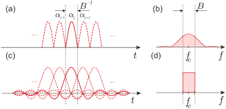
A narrowband scenario with will be considered here. The normalized spectrum of the signal is given by , where is the Fourier transform of the pulse profile . As shown in Fig. 1(b), the slot rate characterizes the extent of the signal spectrum in the frequency domain [25]. The formalism used here includes also the case of wavepackets overlapping in the temporal domain, such as the commonly used sinc profile illustrated with Fig. 1(c)
| (6) |
In this particular case the signal spectrum has a rectangular form depicted in Fig. 1(d) extending from to and the slot rate has direct interpretation of the signal bandwidth.
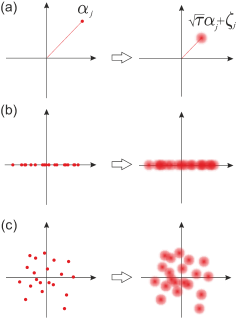
The propagation of the optical signal through the physical medium will be described using the standard AWGN model, in which complex amplitudes of individual pulses undergo a transformation
| (7) |
Here the transmission coefficient specifies the change in the optical signal power in the course of propagation and are random variables that characterize noise added in individual slots. It is important to stress that these variables do not include the noise contributed by the detection process, which will be treated separately. For clarity, the field component contributed by the variables will be referred to as the excess noise. In the AWGN model for the excess noise, are mutually independent complex-valued Gaussian random variables with zero mean and the variances of their real and imaginary parts equal to
| (8) |
The total variance can be interpreted as the mean number of excess noise photons added per one temporal slot. In the white noise scenario, is independent of the slot rate and can be expressed as
| (9) |
where is the excess noise power spectral density. In order to keep the notation concise, the average received signal photon number per slot will be denoted as
| (10) |
When the signal power is attenuated, i.e. , the parameter can assume any nonnegative value. In this regime, loss-only propagation is defined by . However, when the output signal emerges amplified, i.e. , the excess noise must be added in the amount of at least . This requirement can be interpreted within the quantum theory of optical amplification as a consequence of the Heisenberg uncertainty principle [28, 29].
III Conventional detection
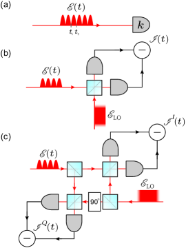
Standard methods to measure the received optical signal are direct detection and homodyne detection of one or both quadratures of the electromagnetic field, shown in Fig. 3. This section will briefly review statistical properties of these measurements assuming that the photodetection process is free from technical imperfections and operates at the shot noise level. The objective is to identify the minimum amount of noise that has to occur in the readout of an optical signal by conventional detection methods.
The standard techniques to measure an optical field are based on the photoelectric effect, when incident light ejects electrons from a photocathode or generates electron-hole pairs in a semiconductor. At the fundamental level the number of produced elementary photocarriers is integer, and with a sufficiently low-noise gain mechanism it can be read out from the photodetection device in such discrete form as the photocount number [30]. Within the framework of the quantum theory of electromagnetic radiation, generation of each photocarrier is associated with an absorption of a single photon from the field illuminating the photodetector [31]. However, equivalent statistical predictions regarding the photodetection process can be obtained by treating the electromagnetic field as a classical entity and using a quantum mechanical model only to describe the charge carriers in the photodetector [32]. Such a semiclassical description of the photodetection process is valid as long as one does not deal with non-classical states of light that cannot be legitimately described within classical electrodynamics.
In an idealized scenario when the photodetector has unit detection efficiency and produces no dark counts, the probability of generating photocarriers over a time interval lasting from to by an incident electromagnetic field with a complex envelope is given by the Poissonian statistics
| (11) |
where the expectation value of the photocount number
| (12) |
can be interpreted as the mean number of photons carried by the field within the measurement interval. The variance of the photocount number is referred to as the shot noise level. Taking in the form given by Eq. (3), when the integration interval contains only the th signal pulse and , the mean photocount number can be identified with the mean number of photons in that pulse, .
Direct detection reveals information only about the intensity of the incident electromagnetic field. A standard phase-sensitive measurement technique is homodyning, where the incoming signal is superposed on a beam splitter with an auxiliary local oscillator (LO) beam that has the same frequency as the signal carrier. We will consider a model of a homodyne setup shown in Fig. 3(b), where LO is prepared as a continuous wave field with a complex amplitude . Both the signal and LO fields are superposed on a balanced 50:50 beam splitter [33] whose output ports are monitored by idealized photodetectors producing photocount statistics described by Eq. (11). The two fields leaving the beam splitter are described by . Let us divide the time axis into discrete intervals of duration indexed using an integer , with the th interval centered at . When the signal and the LO fields do not fluctuate, the joint probability distribution of registering and photocounts on the two photodetectors over the th interval is a product of two Poissonian distributions with respective expectation values
| (13) |
where the second approximate expression holds if is shorter than the temporal variation of the signal field envelope . If the LO field carries a macroscopic number of photons over the integration time , i.e. , the photocount numbers can be treated as continuous variables [34] characterized by normal distributions that approximate Poisson distributions for . Consider now the rescaled differential photocurrent
| (14) |
Under present assumptions the differential photocurrent is a Gaussian random variable with the expectation value
| (15) |
and the variance given by
| (16) |
where only the leading-order terms in have been retained when evaluating . Provided that the signal and the LO fields do not exhibit any fluctuations, the differential photocurrent noise is uncorrelated between different time intervals, for . In the remainder, it will be convenient to apply the limiting transition and treat as a coarse-grained time variable. In this limit
| (17) |
and
| (18) |
Applying to a filter function [35] described in the temporal domain by a normalized real profile yields a quadrature variable
| (19) |
The expectation value of can be directly calculated using Eq. (17) for given by Eq. (3) to be equal to
| (20) |
while Eq. (18) gives variance
| (21) |
When the filter matches the profile of the th signal wavepacket, , Eq. (20) reduces to , which follows from the orthogonality condition (1). This requires that the wavepacket profile is real. By selecting the LO phase or one can detect respectively either the or the field quadrature. Eqs. (20) and (21) imply that the measurement outcome is characterized by a Gaussian probability distribution
| (22) |
Note that the variance of this distribution stems from the shot noise in the photodetection process and its numerical value is determined by the rescaling of the differential photocurrent used in Eq. (14). Remarkably, quadrature distributions have been recently measured at the shot-noise-level for binary phase shift keyed (BPSK) signals sent from a geostationary satellite to an optical ground station equipped with a homodyne receiver [36].
A way to measure both and quadratures for a single pulse is to split the input signal equally between two homodyne setups and to use LO with phases and [37]. This arrangement, known in the context of optical communication as phase diversity homodyne detection [38, 39, 40], is shown in Fig. 3(c). The rescaled differential photocurrents and are defined analogously to Eq. (14) using the LO amplitude fed into an individual homodyne setup and taken in the limit . Their expectation values read:
| (23) |
Note the reduction by a factor compared to Eq. (17), as each homodyne setup receives only half of the input signal power. Differential photocurrent noise is characterized by and . In the case of a two-quadrature measurement one can take a complex normalized filter function and define
| (24) |
When has the form given in Eq. (3) one obtains
| (25) |
and . If matches the profile of the th wavepacket, the joint probability distribution for and can be compactly written as:
| (26) |
Note that in the present case the profile can be complex.
Compared to the one-quadrature measurement described by Eq. (22), the complex amplitude in Eq. (26) is reduced by a factor that stems from dividing the signal power between two homodyne setups, while the variances of individual outcomes and remains at the same level, . In the quantum theory of electromagnetic radiation and quadratures are described by non-commuting observables. Simultaneous measurement of such observables on a single quantum system has to be accompanied by additional uncertainty [41, 42]. This can be viewed as the fundamental reason for the reduced signal-to-noise ratio when both quadratures are detected for one optical pulse.
Importantly, matched filtering allows in principle for shot-noise-level determination of quadratures for individual symbols even in the case of temporally overlapping pulses, provided that the orthogonality condition (1) is satisfied. In contrast, standard direct detection requires that the individual pulses are confined to separate slots in order to discriminate between their contributions to the photocount statistics. This restriction can be in principle lifted using the recently developed technique of quantum pulse gating, which allows one to demultiplex individual temporal wavepackets from an orthogonal set by carefully engineered up-conversion in a nonlinear medium [43, 44, 45].
IV Communication channel
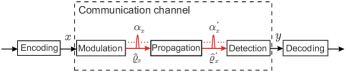
In a generic communication scenario shown in Fig. 4, the complex amplitude for a pulse in a given slot is selected according to the value of an input random variable characterized by a probability distribution . The outcome of the measurement performed at the detection stage is a realization of a certain random variable . In the absence of memory effects the communication channel is characterized by a set of conditional probability distributions . In the optical implementation considered here, these distributions are determined jointly by the map , the transformation of the optical signal in the course of propagation, and the employed detection scheme. The amount of information about that can be recovered from is quantified by the mutual information [46]
| (27) |
where and are respectively the marginal and the conditional entropy of the measurement results. According to Shannon’s noisy-channel coding theorem [47], the maximum amount of information per channel use that can be communicated reliably at an arbitrarily low error rate is obtained by optimizing the mutual information with respect to the input probability distribution . This defines the capacity of a memoryless channel as
| (28) |
A standard illustration of the above concept is the derivation of the Shannon capacity limit. The basic theoretical tool is the Shannon-Hartley theorem [48], which states that the capacity of an analog communication channel with a real input variable and a real output variable related through a Gaussian conditional probability distribution
| (29) |
under the constraint is equal to and is attained by the Gaussian input distribution .
Consider first the case when only one field quadrature, taken for concreteness to be the component, is used for communication. Let the input variable define the complex field amplitude by and . The average power constraint can be expressed as
| (30) |
The last equality follows from Eq. (5) taking into account the fact that in the present scenario the imaginary part of the complex field amplitude is identically set to zero. The explicit form of the conditional distribution (29) can be obtained in the current case by inserting the right hand side of Eq. (7) into Eq. (22) and averaging over the excess noise. The resulting scaling factor is simply the power transmission coefficient for the optical field. The variance is a sum of two contributions. The first one, equal to as implied by (8), stems from the excess noise, while the second one comes from the homodyne measurement itself. If the measurement is carried out at the shot noise level, the latter contribution is according to Eq. (21) and . Consequently, for single-quadrature communication one obtains the Shannon capacity limit in the form
| (31) |
where the enumerator has been expressed in terms of the average received signal photon number per slot defined in Eq. (10).
In the scenario when both and quadratures are used for information transmission, two real variables and are used in each slot and . Given that the average optical power carried by one quadrature is now one has and analogously . The scaling factor between the input variables and and the homodyne measurement outcomes and is as in the present case only half of the input power is directed to each of the two homodyne setups. For the same reason, only half of the excess noise power should be accounted for in the variance . The Shannon capacity in bits per slot for two-quadrature communication is a sum of two equal contributions from and components and reads [49]
| (32) |
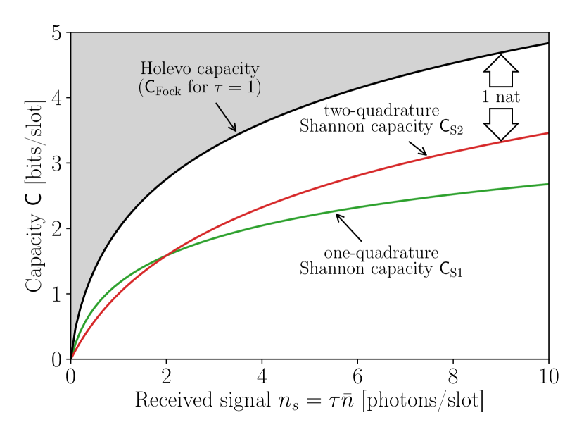
Fig. 5 compares Shannon capacities for one- and two-quadrature encodings as a function of the average received signal photon number for loss-only propagation, when the excess noise is zero , and quadratures are measured at the shot noise level. It is seen that below it is beneficial to use single-quadrature encoding, which however requires a local oscillator phase-locked to the received signal. Around the capacity is in principle optimized by time-sharing between one- and two-quadrature communication [50], but the advantage of this strategy is minuscule.
When excess noise dominates the homodyne shot noise, , one can neglect the latter and and write the Shannon capacity limit in terms of the signal-to-noise ratio (SNR) . In this case, a straightforward comparison of one- and two-quadrature Shannon capacity limits yields
| (33) |
and for any SNR value it is beneficial to use both quadratures for communication. Let us note that the transmission coefficient and the noise density may incorporate respectively the non-unit detection efficiency and the excess noise contributed by the detection process.
The maximum attainable transmission rate in bits per unit time for a given communication scenario is given by
| (34) |
where is the corresponding capacity limit expressed in bits per slot.
V Holevo limit
The Shannon capacity limit reviewed in the preceding section relies on two assumptions. The first one is that the optical field carrying information can be described within the classical theory of electromagnetic radiation using the expression given in Eq. (3). The second one is that the optical signal is detected by means of homodyning, capable of measuring one or both quadratures with shot-noise-level precision. In the case of a lossless channel with unit transmission, , and no excess noise, , there exists a very simple optical communication scenario suggested by Gordon [1] which beats the Shannon limit. Quantum mechanics permits preparation of a light pulse in a state which contains exactly photons, called a photon number state or a Fock state [51]. In recent years, impressive progress in generation of such states has been made in the context of prospective applications in quantum information processing and communication [52, 53, 54]. Suppose that the message to be transmitted is encoded in Fock states, with the -photon Fock state sent with a probability . Because a pulse prepared in an -photon Fock state generates exactly counts on an ideal photodetector with unit detection efficiency and no dark counts, the Fock state transmitted over a lossless channel can be in principle identified unambiguously by direct detection. For such a communication scenario the mutual information reads . In order to identify the capacity in this communication scenario, the above expression needs to be maximized over the probabilities under the average power constraint . This task is a simple exercise in the method of Lagrange multipliers with the result , where
| (35) |
A graph of depicted in Fig. 5 shows that communication with Fock states over a lossless channel exceeds the one- and two-quadrature Shannon capacities for any average signal power. Although this scenario is highly hypothetical due to rather unrealistic technical requirements, it indicates that there are instances when the Shannon formula does not specify the ultimate capacity of optical communication under the average power constraint. In order to identify the ultimate quantum capacity limits, one needs to describe the input states of light, their propagation, as well as the detection of the optical signal using the mathematical formalism of quantum mechanics. Presenting this formalism in full detail would go beyond the scope of the present tutorial paper. We will give here only a brief, few-paragraph summary, referring an interested reader to one of excellent textbooks [55, 56, 57].
Fock states used in the communication scenario proposed by Gordon cannot be legitimately described within the classical theory of electromagnetic radiation. In order to take into account Fock states and any other non-classical states of light, the complex amplitudes representing the electromagnetic field in individual slots need to be replaced by more intricate mathematical objects, namely density operators, denoted often with a carret as and represented by infinitely dimensional, hermitian, positive semidefinite matrices with a unit trace. The counterpart of well-defined complex field amplitudes is the class of coherent states [58, 59]. In the quantum mechanical picture of communication also shown in Fig. 4, the value of the input random variable determines the quantum state of the electromagnetic field in a given slot. Propagation through the physical medium is described by a certain map acting within the set of density operators. In our case, this map is a generalization of the transformation given in Eq. (7). After propagation, the measurement of the received optical signal produces outcomes described by a random variable . The conditional probability distributions of measurement outcomes when the field arrives at the receiver in a state can be found using Born’s rule. This enables one to calculate the mutual information according to Eq. (27).
The ultimate quantum mechanical capacity limit is obtained by optimizing the mutual information in two domains. The first one involves optimization over all measurements—even hypothetical—that can be performed on the received quantum systems. This task is greatly simplified by Holevo’s theorem [16], which states that for any physically permissible measurement one has
| (36) |
where is the von Neumann entropy of a density operator . The Holevo quantity defined above has formal structure analogous to mutual information in Eq. (27). The first term is the von Neumann entropy of the average output quantum state after propagation, while the second term is the average von Neumann entropy of an individual output state whose preparation is known.
In the second step, the Holevo quantity needs to be optimized over all ensembles of input quantum states with respective probabilities that satisfy relevant constraints, in the case considered here an upper bound on the average optical power. A rigorous mathematical proof of the quantum limit for the AWGN propagation model has been presented only recently [20]. The result confirmed the previously conjectured expression in the form:
| (37) |
where has been defined in Eq. (35). In the following, will be referred to as the Holevo capacity limit. Interestingly, for any transmission coefficient and the excess noise value , the Holevo quantity calculated according to Eq. (36) for a continuous Gaussian ensemble of coherent states with complex amplitudes yields the capacity limit . This is a direct counterpart of the input probability distribution saturating the two-quadrature Shannon capacity limit. However, the detection strategy that would achieve the Holevo quantity for this input ensemble remains highly elusive. It has been demonstrated that the inequality in (36) is tight [17, 18, 19], but the argument used in the mathematical proof cannot be translated in a straightforward manner into feasible detection schemes for optical fields. This is somewhat analogous to the canonical proof of the Shannon noisy channel coding theorem based on the statistics of random codes, which does not necessarily provide a constructive recipe to devise practical error correction algorithms.
It is insightful to compare the Holevo capacity limit with the Shannon capacity limit in specialized parameter regimes. In the absence of excess noise, when , one has . Consequently, the curve shown in Fig. 5 as depicts also more generally the Holevo capacity limit for loss-only propagation [60]. Furthermore, for large average received signal photon number per slot, , one obtains the following power series expansion in :
| (38) |
The leading-order term is simply the Shannon capacity of two-quadrature communication derived in Eq. (32) in the special case when there is no excess noise, . The second-to-leading term specifies the capacity advantage compared to the Shannon limit when . This advantage is equal to of information per slot. On the other hand, when the excess noise photon number per slot is much greater than one, , applying expansion (38) to both and yields
| (39) |
It is seen that the terms cancel and the difference between the Holevo capacity and the Shannon capacity becomes minute.
The above results indicate that the Holevo advantage is negligible in scenarios where optical amplification, inevitably generating substantial amounts of excess noise, is used to regenerate propagating optical signals [61, 62]. Unconventional communication strategies can be beneficial for short-haul loss-only links, such as optical interconnects. A newly emerging application area may be continuous-variable quantum key distribution (QKD) [63, 64]. In QKD protocols, generation of a secure cryptographic key requires that the mutual information between the the sender and the receiver exceeds the information about the transmitted signal or measurement outcomes that could be gained by an eavesdropper with unlimited technological capabilities [65]. Increasing the mutual information between the legitimate users could improve the key rates or even enable key generation over longer distances. Another potential use case emerges in scenarios where signal regeneration is fundamentally not possible, such as optical communication in space [66].
VI Photon-starved communication
The difference between the Shannon and the Holevo capacity limits is most strongly pronounced in the photon-starved regime, when the average received number of signal photons per slot is much less than one, . This scenario, encountered e.g. in deep-space optical communication [67, 68, 69, 70], can be viewed as an extreme version of power-limited communication, when received signal power is restricted but the utilized bandwidth is so high that . In this parameter regime it is convenient to express the maximum attainable information rate defined in Eq. (34) as
| (40) |
where is the photon information efficiency (PIE) specifying how much information is retrieved from one received photon [71]. The product is the number of signal photons received in unit time. As a side note, PIE is closely related to the information theoretic concept of the capacity per unit cost which has been analyzed within the classical [72] as well as the quantum mechanical [73, 74] framework.
When , expansion of one- and two-quadrature Shannon capacity limits derived respectively in Eqs. (31) and (32) up to the linear term in yields the following expressions for PIE:
| (41) |
When the excess noise is low, , homodyne shot noise dominates the denominator in both expressions and the PIE is effectively equal to per photon for one-quadrature communication and per photon for two-quadrature communication. For high excess noise, , both expressions in Eq. (41) coincide and are equal to . Reverting to the information rate according to Eq. (40) one obtains the standard formula for power-limited communication in the form .
The above result is in stark contrast with the PIE obtained from the Holevo capacity limit. Consider first loss-only propagation with . For the Holevo capacity limit can be written as a sum of a logarithmic term and a remainder admitting a power series expansion in , which yields:
| (42) |
As illustrated in Fig. 6(a), the above expression exhibits a qualitatively different scaling with compared to the Shannon limit and it can attain an arbitrarily high value with diminishing .
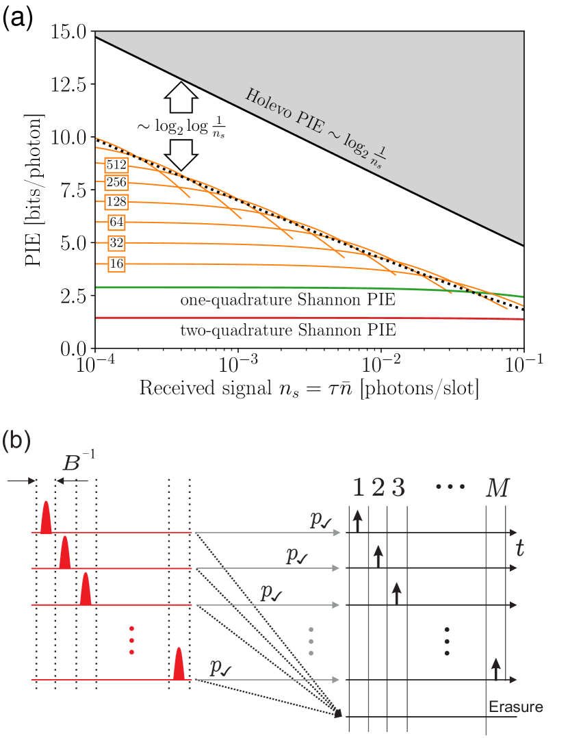
A practical way to achieve high photon information efficiency in optical communications is to use the pulse position modulation (PPM) format combined with direct detection. As depicted in Fig. 6(b), -ary PPM format uses equiprobable multislot symbols defined by the location of one pulse within a frame of otherwise empty temporal slots. Thus one PPM frame can encode bits of information. In order to ensure a fair comparison with other communication scenarios, the duration of a single slot will be kept at . Hence time required to transmit a single PPM symbol is . Under the average power constraint, the pulse carries the optical energy of the entire frame, equal to after transmission. In the absence of excess noise, ideal direct detection allows one to recover the input symbol from the timing of the photodetection event, provided that at least one photocount has been registered. According to Eq. (11) specialized to the present scenario, the probability of such an event is equal to . When no photocount is produced over the entire PPM frame, information about the transmitted symbol is erased. The mutual information per slot for such an -ary erasure communication channel is a product of three factors corresponding respectively to renormalization to one temporal slot, the probability that the erasure has not taken place, and the number of bits encoded in one PPM frame [75]. The resulting PIE is depicted in Fig. 6(a) for PPM orders that are integer powers of . For a given PPM order , in the limit the PIE approaches the value
| (43) |
which follows from the linear approximation . This approximation requires that .
When the average received signal photon number per slot is fixed, one can identify the optimal PPM order by expanding up to the quadratic term
| (44) |
and inserting the result into the expression for given in Eq. (43). Equating to zero the derivative of the resulting approximate with respect to , treated as a continuous real parameter, yields a closed expression for the optimal PPM order in the form [76]
| (45) |
where is the Lambert function [77] defined by the transcendental equation . The corresponding optimal PIE value can be written as [78]
| (46) |
As seen in Fig. 6(a), this expression slightly underestimates the optimal value of PIE. For large arguments the Lambert function admits expansion . Using this expansion in Eq. (46) and comparing the result with the Holevo PIE calculated in Eq. (42) reveals a gap between the PIE of the optimized PPM format with direct detection on one hand and the ultimate quantum limit on the other hand [79]. This gap is characterized in the leading order by a double-logarithmic term of the form .
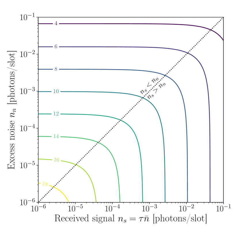
In practice, the propagating optical signal will always acquire some excess noise, contributed e.g. by scattered stray light. Its impact can be estimated using Fig. 7, which depicts the Holevo limit on the photon information efficiency as a function of the signal and the excess noise photon numbers per slot. It is seen that the noiseless analysis holds as long as . For a fixed non-zero excess noise figure , the PIE remains finite with the maximum value attained when :
| (47) |
Thus the general Holevo limit on the maximum attainable information rate in the power-limited regime with unrestricted bandwidth takes the form
| (48) |
Notably, the second expression, involving dimensional physical quantities, depends explicitly on the energy of a single photon at the carrier frequency. This energy defines the absolute scale for the noise power spectral density below which the quantum nature of light starts to play a non-trivial role. Only when one can expand the logarithm into a power series to obtain the Shannon expression .
In the model considered above only excess noise added to the signal wavepacket profile has been taken into account in accordance with Eq. (7). When standard direct detection is used, one should include in the analysis excess noise present in the entire time-bandwidth area measured by the photodetector [80]. In the basic model for such a scenario, when the time-bandwidth area detected per slot is much larger than one, the effective statistics of background counts generated by the excess noise can be described by Poissonian distribution [81]. The photon information efficiency of such a noisy PPM link can be analyzed using a relative entropy bound [82]. If the photodetector discriminates only between zero and at least one photocount in each slot, the dependence of PIE on the signal and the noise strengths has a qualitatively similar character to that shown in Fig. 7 [83, 84]. It is worth noting that the technique of quantum pulse gating [43, 44, 45] can be used as a noise-rejection mechanism for the received optical signal that potentially has both unit efficiency and unit selectivity [85]. This technique combined with photon number resolving photodetection in principle could allow one to approach the Holevo limit in photon-starved communication [86].
VII Joint multisymbol detection
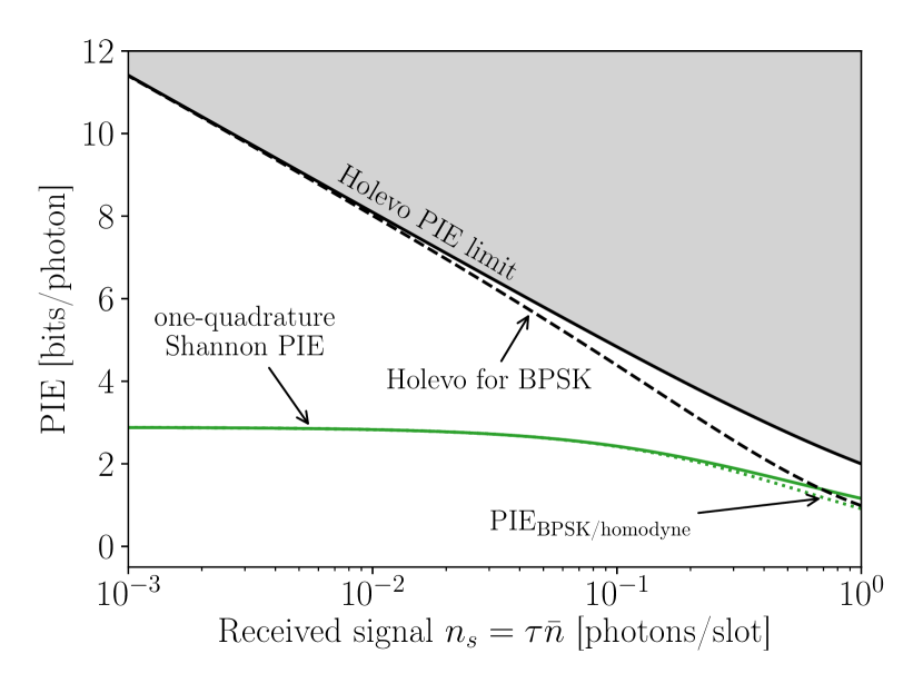
As pointed out in Sec. V, the Holevo theorem does not provide a systematic way to design practical measurements that saturate the Holevo quantity for a given input ensemble of quantum states. Nevertheless, it can motivate search for detection strategies that go beyond conventional approaches. As a simple example, consider the BPSK constellation, represented in the quantum mechanical formalism by two equiprobable coherent states with the same mean photon number and phases and . Loss-only propagation attenuates their amplitudes to , where . In the photon-starved regime, when , shot-noise-level homodyne detection of the quadrature yields PIE that practically overlaps with that implied by the one-quadrature Shannon capacity limit, as shown in Fig. 8. In contrast, the Holevo quantity calculated for the BPSK constellation yields photon information efficiency that is very close to the Holevo capacity limit. This result indicates that photon-efficient communication can be in principle achieved with the BPSK constellation, but conventional homodyning needs to be replaced by another detection strategy.
In general, two prerequisites are required to saturate the Holevo quantity. The first one is that quantum states drawn from the input ensemble are assembled into words transmitted over multiple channel uses (i.e. many temporal slots in the optical scenario discussed here). This is a straightforward analog of classical encoding. However, the second assumption is that collective measurements are performed on blocks of received elementary quantum systems that carry the entire words. Such joint detection strategies can be much more powerful than measurements performed individually on received quantum systems. This is intimately related to the fact that any quantum measurement reveals only partial information about the measured physical system.
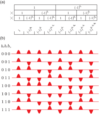
The above aspects can be illustrated with a very elegant communication strategy utilizing the BPSK format that has been described by Guha [87]. The basic idea is to transmit words composed from BPSK symbols defined by rows of a Hadamard matrix. We will refer to these sequences as Hadamard words. Hadamard matrices are real orthogonal matrices with entries and exist for dimensions that are integer powers of 2. The construction of Hadamard words for is shown graphically in Fig. 9(a). The starting point to find the th Hadamard word of length , , is to write in the binary representation using an -bit string so that . The th bit contributes a multiplicative phase factor alternating between and every positions. Individual entries in the th Hadamard word are products of all these factors and determine phases of BPSK symbols in the corresponding Hadamard word, as depicted in Fig. 9(b).
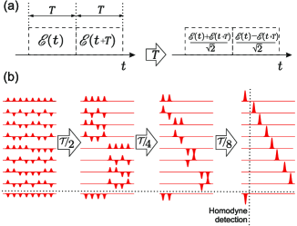
The essence of the joint detection strategy for BPSK Hadamard words is to use optical interference to concentrate the optical energy of the entire word in a location that is different for each input word. This goal can be achieved using a cascade of interferometric modules [88]. As shown schematically in Fig. 10(a), one module superposes the optical field in two adjacent time intervals of duration . Because of the mathematical construction of Hadamard words described above, sending the pulse sequence defined by the th word through a cascade of interferometers that operate on time intervals that correspond to one half, one quarter, etc. fractions of the word duration down to a single temporal slot , concentrates the entire optical energy in the th temporal slot at the output of the cascade, as depicted in Fig. 10(b). If ideal, shot-noise-level direct detection is implemented at this output, the information efficiency is equivalent to that of an -ary PPM link analyzed in Sec. VI. An interesting feature of communication using BPSK Hadamard words is that high PIE is achieved with optical power uniformly distributed across temporal slots, which is in stark contrast with the PPM format. In the latter case increasing PIE requires generating single pulses within frames covering a larger number of temporal slots. This results in a demand for the increasing peak-to-average power ratio of the optical PPM signal, which may be constrained by the physics of the transmitter laser system. In the case of BPSK Hadamard words, the effective format order is increased by changing the phase modulation pattern. The drawback is a much more complex interferometric receiver whose construction depends on the format order.
The fact that detection of individual symbols and postprocessing of measurement outcomes is usually insufficient to saturate the Holevo capacity limit is related to a phenomenon known in quantum information theory as the superadditivity of accessible information [89, 90, 91]. In the case of the BPSK constellation, it can be shown that no physically permissible measurement on individual symbols can beat the PIE limit of bits/photon that is achieved with conventional homodyne detection in the photon-starved regime. Communication with jointly detected BPSK Hadamard words described above can be viewed as an illustration of the superaddivity phenomenon when a collective measurement is performed on at least symbols, as then PIE achieves bits/photon for . Superadditivity of accessible information can be also demonstrated with measurements on fewer than eight phase shift keyed symbols [87, 92, 93, 94]. As an example also shown in Fig. 10(b), consider the set of -ary BPSK Hadamard words enlarged by adding an st sequence . The sequences and are sent with probabilities each, while the remaining Hadamard words are used with the same probability . At the output of the interferometric cascade shown in Fig. 10(b) direct detection is performed in all temporal slots except the first one where the optical energy of the sequences and becomes concentrated. In this slot, homodyning is used to measure the quadrature. The complete detection outcome consists of the continuous quadrature value for the first slot and a discrete variable specifying in which slot, if any, a photocount has occurred. Optimizing mutual information with respect to yields for , and in the limit the respective values of the photon information efficiency , and bits/photon. These figures exceed the Shannon limit as well as the performance of the directly detected PPM format.
VIII Conclusions
The purpose of this tutorial paper was to provide an elementary introduction to quantum mechanical capacity limits of optical communication links. The discussion was based on an elementary model of a narrowband optical signal acquiring excess additive white Gaussian noise in the course of propagation. The crucial issue is the comparison between the excess noise power spectral density and the energy of a single photon at the carrier frequency per unit time-bandwidth area. When , the standard Shannon capacity limit for conventional quadrature measurements is applicable and the performance of a communication link can be characterized in terms of the signal-to-noise ratio.
The situation becomes more nuanced when . In this regime the particle nature of light plays a non-trivial role and the energy of a single photon at the carrier frequency defines the absolute scale for quantifying the signal and the noise strengths. In the discrete slot model used in this tutorial, two relevant figures of merit are the average number of signal and noise photons per slot. The ultimate capacity limit given in Eq. (37) follows from Holevo’s theorem and it depends explicitly on both and rather than their ratio. This reflects the fact that the Holevo capacity limit involves optimization over all physically permissible detection strategies for which no single universal noise figure can be defined. When the average signal photon number per slot significantly exceeds one, , the advantage of the Holevo capacity limit is bits per slot compared to the Shannon limit. So far not much is known about practical designs for receivers that would beat the Shannon limit in this case. In the photon-starved regime, when , photon counting detection of intensity-modulated signals can approach the Holevo capacity limit in the leading order, as exemplified by the PPM format optimized with respect to the frame length.
Many interesting questions arise regarding quantum capacity limits beyond the elementary linear AWGN model considered here. Examples include quantum effects in non-linear signal propagation [95, 96] and unconventional communication strategies in the presence of non-Gaussian noise [97, 98]. Also, adopting a more general perspective on the time-frequency structure of optical signals may inspire novel modulation formats and receiver designs [99, 100].
Acknowledgment
Insightful discussions with Christian Antonelli, René-Jean Essiambre, Saikat Guha, Gerhard Kramer, Christoph Marquardt, Antonio Mecozzi, Mark Shtaif, as well as our collaborators on research projects related to quantum aspects of optical communications, are gratefully acknowledged.
References
- [1] J. P. Gordon, “Quantum effects in communications systems,” Proceedings of the IRE, vol. 50, no. 9, pp. 1898–1908, Sep. 1962.
- [2] L. Mandel and E. Wolf, Optical Coherence and Quantum Optics. Cambridge University, 1995, ch. 9.
- [3] S. Shamai, “Capacity of a pulse amplitude modulated direct detection photon channel,” IEE Proceedings I Communications, Speech and Vision, vol. 137, no. 6, p. 424, 1990.
- [4] J. Shapiro, “Quantum noise and excess noise in optical homodyne and heterodyne receivers,” IEEE Journal of Quantum Electronics, vol. 21, no. 3, pp. 237–250, mar 1985.
- [5] J. Salz, “Modulation and detection for coherent lightwave communications,” IEEE Communications Magazine, vol. 24, no. 6, pp. 38–49, jun 1986.
- [6] K. Kikuchi, “Fundamentals of coherent optical fiber communications,” Journal of Lightwave Technology, vol. 34, no. 1, pp. 157–179, jan 2016.
- [7] J. H. Shapiro, “The quantum theory of optical communications,” IEEE J. Sel. Top. Quant. Electr., vol. 15, no. 6, pp. 1547–1569, 2009.
- [8] C. R. Müller, M. A. Usuga, C. Wittmann, M. Takeoka, C. Marquardt, U. L. Andersen, and G. Leuchs, “Quadrature phase shift keying coherent state discrimination via a hybrid receiver,” New Journal of Physics, vol. 14, no. 8, p. 083009, aug 2012.
- [9] J. Chen, J. L. Habif, Z. Dutton, R. Lazarus, and S. Guha, “Optical codeword demodulation with error rates below the standard quantum limit using a conditional nulling receiver,” Nat. Photonics, vol. 6, pp. 374–379, 2012.
- [10] F. E. Becerra, J. Fan, G. Baumgartner, J. Goldhar, J. T. Kosloski, and A. Migdall, “Experimental demonstration of a receiver beating the standard quantum limit for multiple nonorthogonal state discrimination,” Nat. Photonics, vol. 7, pp. 147–152, 2013.
- [11] H. P. Yuen and M. Ozawa, “Ultimate information carrying limit of quantum systems,” Physical Review Letters, vol. 70, no. 4, pp. 363–366, jan 1993.
- [12] C. M. Caves and P. D. Drummond, “Quantum limits on bosonic communication rates,” Rev. Mod. Phys., vol. 66, pp. 481–537, Apr 1994.
- [13] H. Yuen and J. Shapiro, “Optical communication with two-photon coherent states–part I: Quantum-state propagation and quantum-noise,” IEEE Transactions on Information Theory, vol. 24, no. 6, pp. 657–668, nov 1978.
- [14] Y. Yamamoto and H. A. Haus, “Preparation, measurement and information capacity of optical quantum states,” Rev. Mod. Phys., vol. 58, pp. 1001–1020, Oct 1986.
- [15] E. Davies, “Information and quantum measurement,” IEEE Transactions on Information Theory, vol. 24, no. 5, pp. 596–599, sep 1978.
- [16] A. S. Holevo, “Bounds for the quantity of information transmitted by a quantum communication channel,” Problems of Information Transmission, vol. 9, no. 3, pp. 177–183, 1973.
- [17] P. Hausladen, R. Jozsa, B. Schumacher, M. Westmoreland, and W. K. Wootters, “Classical information capacity of a quantum channel,” Phys. Rev. A, vol. 54, pp. 1869–1876, Sep 1996.
- [18] B. Schumacher and M. D. Westmoreland, “Sending classical information via noisy quantum channels,” Phys. Rev. A, vol. 56, pp. 131–138, Jul 1997.
- [19] A. S. Holevo, “The capacity of the quantum channel with general signal states,” IEEE Transactions on Information Theory, vol. 44, no. 1, pp. 269–273, 1998.
- [20] V. Giovannetti, R. García-Patrón, N. J. Cerf, and A. S. Holevo, “Ultimate classical communication rates of quantum optical channels,” Nature Photon., vol. 8, pp. 796–800, 2014.
- [21] A. Holevo and R. Werner, “Evaluating capacities of bosonic gaussian channels,” Physical Review A, vol. 63, no. 3, feb 2001.
- [22] V. Giovannetti, S. Guha, S. Lloyd, L. Maccone, and J. H. Shapiro, “Minimum output entropy of bosonic channels: A conjecture,” Physical Review A, vol. 70, no. 3, sep 2004.
- [23] R. García-Patrón, C. Navarrete-Benlloch, S. Lloyd, J. H. Shapiro, and N. J. Cerf, “Majorization theory approach to the gaussian channel minimum entropy conjecture,” Physical Review Letters, vol. 108, no. 11, mar 2012.
- [24] J. Kahn and K.-P. Ho, “Spectral efficiency limits and modulation/detection techniques for DWDM systems,” IEEE Journal of Selected Topics in Quantum Electronics, vol. 10, no. 2, pp. 259–272, mar 2004.
- [25] R.-J. Essiambre, G. Kramer, P. J. Winzer, G. J. Foschini, and B. Goebel, “Capacity limits of optical fiber networks,” Journal of Lightwave Technology, vol. 28, no. 4, pp. 662–701, feb 2010.
- [26] P. J. Winzer, “High-spectral-efficiency optical modulation formats,” Journal of Lightwave Technology, vol. 30, no. 24, pp. 3824–3835, dec 2012.
- [27] P. Bayvel, R. Maher, T. Xu, G. Liga, N. A. Shevchenko, D. Lavery, A. Alvarado, and R. I. Killey, “Maximizing the optical network capacity,” Philosophical Transactions of the Royal Society A: Mathematical, Physical and Engineering Sciences, vol. 374, no. 2062, p. 20140440, mar 2016.
- [28] H. A. Haus and J. A. Mullen, “Quantum noise in linear amplifiers,” Physical Review, vol. 128, no. 5, pp. 2407–2413, dec 1962.
- [29] C. M. Caves, “Quantum limits on noise in linear amplifiers,” Phys. Rev. D, vol. 26, pp. 1817–1839, Oct 1982.
- [30] L. Mandel, “Fluctuations of photon beams: The distribution of the photo-electrons,” Proceedings of the Physical Society, vol. 74, no. 3, pp. 233–243, sep 1959.
- [31] P. L. Kelley and W. H. Kleiner, “Theory of electromagnetic field measurement and photoelectron counting,” Phys. Rev., vol. 136, pp. A316–A334, Oct 1964.
- [32] L. Mandel, “Photoelectric counting measurements as a test for the existence of photons,” Journal of the Optical Society of America, vol. 67, no. 8, p. 1101, aug 1977.
- [33] H. P. Yuen and V. W. S. Chan, “Noise in homodyne and heterodyne detection,” Optics Letters, vol. 8, no. 3, p. 177, mar 1983.
- [34] H. Yuen and J. Shapiro, “Optical communication with two-photon coherent states–part III: Quantum measurements realizable with photoemissive detectors,” IEEE Transactions on Information Theory, vol. 26, no. 1, pp. 78–92, jan 1980.
- [35] A. Mecozzi and R.-J. Essiambre, “Nonlinear Shannon limit in pseudolinear coherent systems,” J. Lightwave Technol., vol. 30, no. 12, pp. 2011–2024, Jun 2012.
- [36] K. Günthner, I. Khan, D. Elser, B. Stiller, Ömer Bayraktar, C. R. Müller, K. Saucke, D. Tröndle, F. Heine, S. Seel, P. Greulich, H. Zech, B. Gütlich, S. Philipp-May, C. Marquardt, and G. Leuchs, “Quantum-limited measurements of optical signals from a geostationary satellite,” Optica, vol. 4, no. 6, pp. 611–616, Jun 2017.
- [37] N. G. Walker and J. E. Carroll, “Multiport homodyne detection near the quantum noise limit,” Optical and Quantum Electronics, vol. 18, no. 5, pp. 355–363, sep 1986.
- [38] R. Noe, “PLL-free synchronous QPSK polarization multiplex/diversity receiver concept with digital I&Q baseband processing,” IEEE Photonics Technology Letters, vol. 17, no. 4, pp. 887–889, apr 2005.
- [39] D.-S. Ly-Gagnon, S. Tsukamoto, K. Katoh, and K. Kikuchi, “Coherent detection of optical quadrature phase-shift keying signals with carrier phase estimation,” Journal of Lightwave Technology, vol. 24, no. 1, pp. 12–21, jan 2006.
- [40] K. Kikuchi, “Phase-diversity homodyne detection of multilevel optical modulation with digital carrier phase estimation,” IEEE Journal of Selected Topics in Quantum Electronics, vol. 12, no. 4, pp. 563–570, jul 2006.
- [41] E. Arthurs and J. L. Kelly, “On the simultaneous measurement of a pair of conjugate observables,” Bell System Technical Journal, vol. 44, no. 4, pp. 725–729, apr 1965.
- [42] K. Wódkiewicz, “Operational approach to phase-space measurements in quantum mechanics,” Physical Review Letters, vol. 52, no. 13, pp. 1064–1067, mar 1984.
- [43] B. Brecht, D. V. Reddy, C. Silberhorn, and M. G. Raymer, “Photon temporal modes: A complete framework for quantum information science,” Phys. Rev. X, vol. 5, no. 4, p. 041017, 2015.
- [44] M. Allgaier, V. Ansari, L. Sansoni, C. Eigner, V. Quiring, R. Ricken, G. Harder, B. Brecht, and C. Silberhorn, “Highly efficient frequency conversion with bandwidth compression of quantum light,” Nature Communications, vol. 8, no. 1, jan 2017.
- [45] D. V. Reddy and M. G. Raymer, “High-selectivity quantum pulse gating of photonic temporal modes using all-optical Ramsey interferometry,” Optica, vol. 5, no. 4, p. 423, apr 2018.
- [46] T. M. Cover and J. A. Thomas, Elements of Information Theory. John Wiley & Sons, Inc., 2001.
- [47] C. E. Shannon, “A mathematical theory of communication,” Bell System Technical Journal, vol. 27, pp. 379–423, 623–656, 1948.
- [48] ——, “Communication in the presence of noise,” Proc. IRE, vol. 37, no. 1, pp. 10–21, 1949.
- [49] M. J. W. Hall, “Gaussian noise and quantum-optical communication,” Physical Review A, vol. 50, no. 4, pp. 3295–3303, oct 1994.
- [50] M. Takeoka and S. Guha, “Capacity of optical communication in loss and noise with general quantum Gaussian receivers,” Phys. Rev. A, vol. 89, p. 042309, Apr 2014.
- [51] U. Leonhardt, Essential Quantum Optics. Cambridge University Press, 2009.
- [52] A. I. Lvovsky, H. Hansen, T. Aichele, O. Benson, J. Mlynek, and S. Schiller, “Quantum state reconstruction of the single-photon Fock state,” Physical Review Letters, vol. 87, no. 5, jul 2001.
- [53] E. Waks, E. Diamanti, and Y. Yamamoto, “Generation of photon number states,” New Journal of Physics, vol. 8, p. 4, jan 2006.
- [54] M. Cooper, L. J. Wright, C. Söller, and B. J. Smith, “Experimental generation of multi-photon Fock states,” Optics Express, vol. 21, no. 5, p. 5309, feb 2013.
- [55] M. A. Nielsen and I. L. Chuang, Quantum Computation and Quantum Information. Cambridge University Press, 2000.
- [56] E. Desurvire, Classical and Quantum Information Theory. Cambridge University Press, 2009.
- [57] M. M. Wilde, Quantum Information Theory. Cambridge University Press, 2017.
- [58] R. J. Glauber, “Coherent and incoherent states of the radiation field,” Physical Review, vol. 131, no. 6, pp. 2766–2788, sep 1963.
- [59] E. C. G. Sudarshan, “Equivalence of semiclassical and quantum mechanical descriptions of statistical light beams,” Phys. Rev. Lett., vol. 10, pp. 277–279, Apr 1963.
- [60] V. Giovannetti, S. Guha, S. Lloyd, L. Maccone, J. H. Shapiro, and H. P. Yuen, “Classical capacity of the lossy bosonic channel: The exact solution,” Phys. Rev. Lett., vol. 92, p. 027902, Jan 2004.
- [61] C. Antonelli, A. Mecozzi, M. Shtaif, and P. J. Winzer, “Quantum limits on the energy consumption of optical transmission systems,” Journal of Lightwave Technology, vol. 32, no. 10, pp. 1853–1860, may 2014.
- [62] M. Jarzyna, R. Garcia-Patron, and K. Banaszek, “Ultimate capacity limit of a multi-span link wirth phase-insensitive amplification,” in 45th European Conference on Optical Communication, Dublin, Ireland, Sep. 2019.
- [63] C. Silberhorn, T. C. Ralph, N. Lütkenhaus, and G. Leuchs, “Continuous variable quantum cryptography: Beating the 3 dB loss limit,” Physical Review Letters, vol. 89, no. 16, sep 2002.
- [64] F. Grosshans, G. V. Assche, J. Wenger, R. Brouri, N. J. Cerf, and P. Grangier, “Quantum key distribution using gaussian-modulated coherent states,” Nature, vol. 421, no. 6920, pp. 238–241, jan 2003.
- [65] P. Jouguet, S. Kunz-Jacques, E. Diamanti, and A. Leverrier, “Analysis of imperfections in practical continuous-variable quantum key distribution,” Physical Review A, vol. 86, no. 3, sep 2012.
- [66] H. Hemmati, A. Biswas, and I. B. Djordjevic, “Deep-space optical communications: Future perspectives and applications,” Proc. IEEE, vol. 99, no. 11, pp. 2020–2039, 2011.
- [67] H. Hemmati, Deep-Space Optical Communication. John Wiley & Sons, Inc., 2005.
- [68] A. Biswas, M. Srinivasan, R. Rogalin, S. Piazzolla, J. Liu, B. Schratz, A. Wong, E. Alerstam, M. Wright, W. T. Roberts, J. Kovalik, G. Ortiz, A. Na-Nakornpanom, M. Shaw, C. Okino, K. Andrews, M. Peng, D. Orozco, and W. Klipstein, “Status of NASA’s deep space optical communication technology demonstration,” in 2017 IEEE International Conference on Space Optical Systems and Applications (ICSOS), Nov 2017, pp. 23–27.
- [69] Z. Sodnik, C. Heese, P. Arapoglou, K. Schulz, I. Zayer, R. Daddato, and S. Kraft, “Deep-space optical communication system (DOCS) for ESA’s space weather mission to Lagrange orbit L5,” in 2017 IEEE International Conference on Space Optical Systems and Applications (ICSOS), Nov 2017, pp. 28–33.
- [70] D. M. Boroson, “On achieving high performance optical communications from very deep space,” in Free-Space Laser Communication and Atmospheric Propagation XXX, H. Hemmati and D. M. Boroson, Eds., vol. 10524. SPIE, feb 2018, p. 105240B.
- [71] S. Dolinar, K. M. Birnbaum, B. I. Erkmen, and B. Moision, “On approaching the ultimate limits of photon-efficient and bandwidth-efficient optical communication,” in 2011 International Conference on Space Optical Systems and Applications (ICSOS). IEEE, may 2011.
- [72] S. Verdu, “On channel capacity per unit cost,” IEEE Trans. Inf. Theor., vol. 36, no. 5, p. 1019, 1990.
- [73] M. Jarzyna, “Classical capacity per unit cost for quantum channels,” Phys. Rev. A, vol. 96, no. 3, p. 032340, 2017.
- [74] D. Ding, D. S. Pavlichin, and M. M. Wilde, “Quantum channel capacities per unit cost,” IEEE Transactions on Information Theory, vol. 65, no. 1, pp. 418–435, jan 2019.
- [75] A. Waseda, M. Sasaki, M. Takeoka, M. Fujiwara, M. Toyoshima, and A. Assalini, “Numerical evaluation of PPM for deep-space links,” J. Opt. Commun. Netw., vol. 3, no. 6, pp. 514–521, 2011.
- [76] M. Jarzyna, P. Kuszaj, and K. Banaszek, “Incoherent on-off keying with classical and non-classical light,” Opt. Express, vol. 23, no. 3, pp. 3170–3175, 2015.
- [77] R. M. Corless, D. E. G. Gonnet, G. H. anmd Hare, D. J. Jeffrey, and D. E. Knuth, “On the Lambert W function,” Advances in Computational Mathematics, vol. 5, pp. 329–359, 1996.
- [78] M. Jarzyna and K. Banaszek, “Efficiency of optimized pulse position modulation with noisy direct detection,” in Proceedings of the IEEE International Conference on Satellite Optical Systems and Applications (ICSOS), 2017, pp. 176–181.
- [79] Y. Kochman, L. Wang, and G. W. Wornell, “Toward photon-efficient key distribution over optical channels,” IEEE Trans. Inf. Theory, vol. 60, no. 8, pp. 4958–4972, 2014.
- [80] D. M. Boroson, “Performance limits and simplified analysis of photon-counted noisy free-space optical links,” in Free-Space Laser Communication and Atmospheric Propagation XXX, H. Hemmati and D. M. Boroson, Eds. SPIE, feb 2018.
- [81] R. M. Gagliardi and S. Karp, Optical Communications 2nd ed. John Wiley & Sons, 1995.
- [82] J. Hamkins, M. Klimesh, R. J. McEliece, and B. Moision, “Capacity of the generalized PPM channel,” in Proceedings of the International Symposium on Information Theory (ISIT), 2004, pp. 334–334.
- [83] W. Zwoliński, M. Jarzyna, and K. Banaszek, “Range dependence of an optical pulse position modulation link in the presence of background noise,” Opt. Express, vol. 26, no. 20, pp. 25 827–25 838, 2018.
- [84] K. Banaszek, W. Zwoliński, L. Kunz, and M. Jarzyna, “Photon efficiency limits in the presence of background noise,” in Proceedings of the 2019 IEEE International Conference on Space Optical Systems and Applications (ICSOS), Portland, OR, USA, 2019.
- [85] A. Shahverdi, Y. M. Sua, L. Tumeh, and Y.-P. Huang, “Quantum parametric mode sorting: Beating the time-frequency filtering,” Scientific Reports, vol. 7, no. 1, p. 6495, jul 2017.
- [86] K. Banaszek, L. Kunz, M. Jarzyna, and M. Jachura, “Approaching the ultimate capacity limit in deep-space optical communication,” in Free-Space Laser Communications XXXI, H. Hemmati and D. M. Boroson, Eds., vol. 10910. SPIE, mar 2019, p. 109100A.
- [87] S. Guha, “Structured optical receivers to attain superadditive capacity and the Holevo limit,” Phys. Rev. Lett., vol. 106, no. 24, p. 240502, 2011.
- [88] K. Banaszek and M. Jachura, “Structured optical receivers for efficient deep-space communication,” in 2017 IEEE International Conference on Space Optical Systems and Applications (ICSOS), Nov 2017, pp. 34–37.
- [89] M. Sasaki, K. Kato, M. Izutsu, and O. Hirota, “Quantum channels showing superadditivity in classical capacity,” Physical Review A, vol. 58, no. 1, pp. 146–158, jul 1998.
- [90] J. R. Buck, S. J. van Enk, and C. A. Fuchs, “Experimental proposal for achieving superadditive communication capacities with a binary quantum alphabet,” Physical Review A, vol. 61, no. 3, feb 2000.
- [91] H. W. Chung, S. Guha, and L. Zheng, “Superadditivity of quantum channel coding rate with finite blocklength joint measurements,” IEEE Trans. Inf. Theor., vol. 62, no. 10, pp. 5938 – 5959, July 2016.
- [92] A. Klimek, M. Jachura, W. Wasilewski, and K. Banaszek, “Quantum memory receiver for superadditive communication using binary coherent states,” J. Mod. Opt., vol. 63, no. 20, pp. 2074–2080, 2016.
- [93] M. Rosati, A. Mari, and V. Giovannetti, “Multiphase Hadamard receivers for classical communication on lossy bosonic channels,” Phys. Rev. A, vol. 94, no. 6, p. 062325, 2016.
- [94] L. Kunz, M. Jarzyna, W. Zwolinski, and K. Banaszek, “Low-cost limit of classical communication with restricted quantum measurements,” 2019, arxiv:1911.063355 [quant-ph].
- [95] J. F. Corney, J. Heersink, R. Dong, V. Josse, P. D. Drummond, G. Leuchs, and U. L. Andersen, “Simulations and experiments on polarization squeezing in optical fiber,” Physical Review A, vol. 78, no. 2, aug 2008.
- [96] L. Kunz, M. G. A. Paris, and K. Banaszek, “Noisy propagation of coherent states in a lossy kerr medium,” Journal of the Optical Society of America B, vol. 35, no. 2, p. 214, jan 2018.
- [97] J. Trapani, B. Teklu, S. Olivares, and M. G. A. Paris, “Quantum phase communication channels in the presence of static and dynamical phase diffusion,” Physical Review A, vol. 92, no. 1, jul 2015.
- [98] M. T. DiMario, L. Kunz, K. Banaszek, and F. E. Becerra, “Optimized communication strategies with binary coherent states over phase noise channels,” npj Quantum Information, vol. 5, no. 1, jul 2019.
- [99] I. A. Burenkov, O. V. Tikhonova, and S. V. Polyakov, “Quantum receiver for large alphabet communication,” Optica, vol. 5, no. 3, p. 227, feb 2018.
- [100] K. Banaszek, M. Jachura, and W. Wasilewski, “Utilizing time-bandwidth space for efficient deep-space communication,” in International Conference on Space Optics (ICSO) 2018, Z. Sodnik, N. Karafolas, and B. Cugny, Eds., vol. 11180. Proc. SPIE, Jul. 2019, p. 111805X.