Multiple Metric Learning for Structured Data

Abstract

We address the problem of merging graph and feature-space information while learning a metric from structured data. Existing algorithms tackle the problem in an asymmetric way, by either extracting vectorized summaries of the graph structure or adding hard constraints to feature-space algorithms.
Following a different path, we define a metric regression scheme where we train metric-constrained linear combinations of dissimilarity matrices. The idea is that the input matrices can be pre-computed dissimilarity measures obtained from any kind of available data (e.g. node attributes or edge structure). As the model inputs are distance measures, we do not need to assume the existence of any underlying feature space. Main challenge is that metric constraints (especially positive definiteness and sub-additivity), are not automatically respected if, for example, the coefficients of the linear combination are allowed to be negative. Both positive and sub-additive constraints are linear inequalities, but the computational complexity of imposing them scales as $O(D^{3})$, where $D$ is the size of the input matrices (i.e. the size of the data set). This becomes quickly prohibitive, even when $D$ is relatively small. We propose a new graph-based technique for optimizing under such constraints and show that, in some cases, our approach may reduce the original computational complexity of the optimization process by one order of magnitude. Contrarily to existing methods, our scheme applies to any (possibly non-convex) metric-constrained objective function.

Keywords

multiple-metric learning, structured data, nearest neighbours algorithm, metric-constrained optimization.

1 Introduction

1.1 Motivation

In many applications, e.g. social networks analysis, data sets are structured objects consisting of text, real or Boolean high dimensional vectors and a graph. Text and vectors usually provide a description of the real-world entities represented by the graph nodes, while the edge structure is associated with some kind of relationship between them. Through standard word-embedding techniques, it is possible, and also pretty efficient, to transform node-related texts to vectors. Word-embedding vectors can then be merged with real-valued node attributes by opportunely enlarging the feature space. Taking into account the graph edge structure is in general less straightforward. This because, in most cases, the complex relationships represented by graph links cannot be reduced to simple Euclidean distances defined over an explicit feature space.

Goal of this work is to present a new and general method for learning statistical models from graph-structured data sets. We exploit some crucial properties of metric spaces to define an optimization scheme that encodes the whole knowledge provided by a data set into a single mathematical object. Obtained from both node and edge features, the latter can be seen as the metric of the entire data set. The obtained data-set metric can be used directly to solve classical machine learning tasks through extremely simple algorithms such as $(k=1)$ Nearest Neighbor or K-Means algorithms.

The inspiring general idea is that real-world systems (e.g. social networks, financial markets or power energy grids) can be represented in a geometric way by abstract (and not necessarily Euclidean) manifolds. Data points obtained from the systems sit on such abstract manifolds and can be used to detect their underlying (metric) structure. In the machine learning literature, the task of inferring metric structures from data is referred to as the metric learning problem. In the same context, multiple metric learning is a promising and recent extension of the classical metric learning setup where the task is to optimize linear combinations of different distance measures.

Existing approaches mostly focus on Mahalanobis metrics. In that case, data points are mapped to feature vectors lying on a high dimensional space. As the high-dimensional space is usually equipped with a flat Euclidean metric, metric learning reduces to inferring an optimal linear transformation between the original data points and such high dimensional vectors. Advantages of the Mahalanobis approach are the convexity of the optimization problem and the fact that the output is automatically guaranteed to be a metric, e.g. it is positive semi-definite and fulfils all triangle inequalities $M_{ij}\leq M_{ik}+M_{kj}$ ($i,j,k=1,\dots,D$). Technically, this happens because the feature-space metric is defined by $M_{ij}=\|x^{(i)}-x^{(j)}\|^{2}$($i,j=1,\dots,D$), where $x^{(i)}$ are the high-dimensional representatives of the data points and $\|x\|^{2}=x^{T}x$ is the Euclidean norm, which satisfies the triangle inequality by definition.

As mentioned above, however, methods based on Euclidean distances struggle when the input data set contains structured information. The reason is that graph edges are not always defined as Euclidean distances between explicit feature-space vectors, i.e. it does not always exist $\{z^{(i)}\in{\mathbf{R}}^{N}\}_{i=1}^{D}$ ($N\in{\mathbf{N}}_{+}$) such that $M_{ij}=\|z^{(i)}-z^{(j)}\|^{2}$ for all (given) edge weights $M_{ij}$ ($i,j=1,\dots,D$) . We tackle this problem by proposing a two-step scheme where we first extract a set of metrics from the structured data set (e.g. one distinct metric for each different piece of information in the data set) and then consistently combine them into an optimal mixture by solving a metric-constrained optimization process.

1.2 Related work

Metric constraints as a regularization scheme

Metric constraints can be looked at as an interpretable regularization scheme to reduce the complexity of a statistical model. Practical implementations of this idea have already appeared in different domains. It is widely known, for example, that imposing metric constraints in k-means clustering can be highly effective in terms of computational complexity and accuracy of the output (Xing et al.,, 2003; Bilenko et al.,, 2004; Weinberger and Saul,, 2009). More broadly, dissimilarity measures and metrics have been shown to be important for shape analysis (Basri et al.,, 1998), object recognition (Bronstein et al.,, 2007) and features selection (Laub and MÞller,, 2004). Mémoli, (2011) analyzes the role of metrics in data science and discusses their interpretation as summaries of complex datasets.

Metric learning and structured data

The task of unveiling the metric structure of a given set of observations is known in the literature as metric learning (Kulis et al.,, 2013) and has many practical applications (see Yu et al., (2006) or Hoi et al., (2006) for an example in computer vision). The connection with graphs and structured data have also been investigated in the past. Hauberg et al., (2012) focuses on computing geodesic on a feature space where the metric is defined as the superposition of metrics. This is similar to our approach but the formulation of Hauberg et al., (2012) only applies to continuous feature spaces. The paper also shows that being a non-metric may have effects on certain applications. Shi et al., (2014) is a work very close to ours. The authors explain how to learn combinations of global and local metrics. They apply the scheme to multi-task learning problems, which may be solved in a very similar way through the approach proposed here. There are, however, few important differences: i) the paper focuses on Mahalanobis metrics, and hence assume the existence of an Euclidean feature space; ii) the optimized linear combinations have only non-negative weights, which means that the output is guaranteed to be a metric. As in our experiments, the authors evaluate their method through a simple Nearest Neighbor algorithm. Shaw et al., (2011) is an example of how the graph structure can be enforced imposing by hard constraints. The learning task considered in Shaw et al., (2011) is slightly different (the authors learn a metric “such that points connected in the network are close and points which are unconnected are more distant.”) but the same approach may be used in different setups without major modifications. Shaw and Jebara, (2009) presents one of the several existing algorithms for embedding graphs in Euclidean spaces. In that work, the embedding is guaranteed to be low dimensional and to preserve the global topological properties of the input graph. Our approach does not need any embedding step but comparing our method to those approaches would be interesting. Bellet et al., (2013) is a good survey of metric learning methods that assume the existence of an underlying feature space. Many of these rely on converting structured objects to feature vectors through various techniques (as for example the string kernel method of Lodhi et al., (2002) or the bag-of-words approach of Salton et al., (1975) and Fei-Fei and Perona, (2005)). Section 5 of Bellet et al., (2013) contains an exhaustive list of metric learning algorithms that can handle structured data without an explicit vector representation. Most of these algorithms, however, are designed specifically for text-based data and exploit some very peculiar features of the ‘edit distance’.

Metric-constrained optimization

Metric learning is closely related but not equivalent to metric-constrained optimization. As mentioned above metric learning is the problem of inferring a distance measure from a given set of observations (Xing et al.,, 2003; Kulis et al.,, 2013). In the classical setup of metric learning, the starting point is an accessible feature space (from which the target metric is built). Metric-constrained optimization problems includes the more general situation where the feature space can be implicit or not accessible. A more similar problem is multidimensional scaling, where the task is to find N low-dimensional points such that their distances respect a set of given dissimilarity relationships (Cox and Cox,, 2000). In a typical metric-constrained optimization problem, however, the variable is another implicit distance measure and not an explicit low-dimensional features (as in multidimensional scaling). In Veldt et al., (2018) is one of the few example of work about metric-constrained optimization. The authors propose a projection method based on the Dikjstra algorithm (Dykstra,, 1983) and test it on various tasks, such as correlation clustering (Batra et al.,, 2008), sparsest or maximum cut and the metric nearness problem (see below). All these applications can be reformulated as a linear or quadratic programming with $O(N^{3})$ triangle-inequality linear constraints. Roth et al., (2003) is another work that explicitly addresses a metric-constrained optimization problem. In that case, metric constraints are enforced by learning a global transformation of a given set of pairwise distances. Optimization under triangle-inequality constraints have also appeared in various management applications (Igelmund and Radermacher,, 1983; Hanson and Martin,, 1990), but mostly for integer programming (Burdet and Johnson,, 1975).

Intrinsic metrics

The use of intrinsic and extrinsic features of a given data set has been used for improving the performance of various algorithms. Bronstein et al., (2007) contains an interesting comparison between intrinsic and extrinsic similarities, in the framework of shape analysis. A more contextualized description of intrinsic metrics in data science can be found in Keller, (2015). Here we refer to a special case of discrete intrinsic metric, also known as path-length distance. See for example Buckley and Harary, (1990); Diestel, (2018); West et al., (2001) or Bandelt and Chepoi, (2008) for a general survey on graph metrics. A crucial feature of path-length distances is that they automatically respect all triangle inequalities. Actually, they are the discrete versions of intrinsic metrics defined over continuous spaces, which are often used to characterize a manifold without choosing a particular embedding space (see for Burago et al., (2001) or Bridson and Haefliger, (2013) for more details).

Multiple kernel learning

Multiple kernel learning (see for example Lanckriet et al., (2004)) has some strong analogy with our approach. What makes metric learning more challenging is the presence of the $O(D^{3})$ triangle-inequality constraints. As for metrics, the positive definiteness constraint of multiple kernel learning is automatically satisfied when the output is a linear combination with non-negative weights. In our work, we focus for simplicity on linear combinations of metrics but drop the non-negativity restriction to show the potential generality of the approach.

Metric nearness problem

The task of finding the closest metric to a given dissimilarity matrix has been called the metric nearness problem. A triangle-fixing algorithm for solving this specific problem is proposed and analyzed theoretically in Brickell et al., (2008). Based on this, Veldt et al., (2018) introduces a more general metric-projection algorithm to solve linear and quadratic optimization problems.

2 Methods

Notation

We use capital letters with lowercase indexes for matrices, e.g. $X_{ij}=[X]_{ij}$ ($i,j=1,\dots,D$). Lowercase letters with capital indexes are used for their vectorized form, i.e. $x_{I}=[{\rm vec}(X)]_{I}$ ($I=1,\dots,D^{2}$) and $X_{ij}=x_{I}$ for $I=D(i-1)+j$. Element wise product is denoted by “$\circ$” and the transpose of $x$ by $x^{T}$. ${\cal M}_{D}\subset{\mathbf{R}}^{D\times D}$ is the space of $D\times D$ metrics, i.e. the space of real matrices that obey all metric constraints (4). The following short notation is used for linear combinations of matrices $M_{\alpha}=\sum_{r=1}^{R}\alpha_{r}M_{r}\in{\mathbf{R}}^{D\times D}$ and vectors $m_{\alpha}=\sum_{r=1}^{R}\alpha_{r}m_{r}\in{\mathbf{R}}^{D^{2}}$. Given a symmetric matrix, $A=A^{T}$, ${\cal G}(A)$ is the undirected graph obtained by interpreting $A$ as the graph adjacency matrix. $\Gamma_{ij}=\Gamma_{ij}({\cal G})$ is the set of simple paths connecting nodes $i$ and $j$ on ${\cal G}$. Let $p$ be a path on ${\cal G}$, then $\gamma=\gamma(p)\in\{0,1\}^{D^{2}}$ is the vector (unordered) representation of $p$ defined by

$$\left[\gamma(p)\right]_{I}=\left\{\begin{array}[]{ll}1&{\rm if\ }{\rm link}_{i\to j}\in p{\rm\ and\ }I=D(i-1)+j\\ 0&{\rm otherwise}\end{array}\right.,$$ (3)

where ${\rm link}_{i\to j}$ is the link between nodes $i$ and $j$ on ${\cal G}$. As a consequence, the length of $p$ on ${\cal G}(A)$ is $\gamma^{T}m$. More generally, the path-distance between nodes $i$ and $j$ on graph ${\cal G}$ is defined by ${\rm dist}_{\rm path}(i,j,{\cal G})=\min_{{\rm path}\in\Gamma_{ij}({\cal G})}{\rm length}({\rm path})$. $\nabla f$ is th he gradient of $f:{\mathbf{R}}^{N}\to{\mathbf{R}}$ defined by $[\nabla f]_{r}=\frac{\partial f(x)}{\partial x_{r}}$. The ‘softplus’ function and its derivatives are ${\rm softplus}(x)=\log(1+e^{x})$, $\partial_{x}{\rm softplus}(x)=\sigma(x)=(1+e^{-x})^{-1}$ and $\partial_{x}\sigma(x)=\sigma^{\prime}(x)$ and apply element wise to matrices and vectors.

2.1 Metric spaces

A discrete metric space is a discrete set, ${\cal D}=\{x^{(i)}\}_{i=1}^{D}$, and a metric, $M\in{\cal M}$, defined on ${\cal D}$. $M$ is a metric on ${\cal D}$ if

$$M_{ij} = M_{ji},$$ (4)

$$M_{ij} > 0{\rm\ if}\ i\neq j,$$

$$M_{ii} = 0$$

$$M_{ij} \leq M_{ik}+M_{kj},$$

for all $i,j,k=1,\dots,D$. The last inequality is referred to as triangle inequality. $M\in{\cal M}$ can be seen as the adjacency matrix of a fully-connected, undirected and weighted graph, ${\cal G}(M)$. Conversely, given a connected (but not necessarily fully-connected) graph, ${\cal G}$, it is always possible to define a metric over its node set by letting

$$\tilde{M}_{ij}={\rm dist}_{\rm path}(i,j,{\cal G}),$$ (5)

for all $i,j=1,\dots,D$. In this case, $\tilde{M}$ is the intrinsic metric of ${\cal G}$. It is easy to verify that $\tilde{M}\in{\cal M}$. A metric space, $({\cal D},M)$ is a length metric space if $M=\tilde{M}$. For example, ${\mathbf{R}}^{N}$ equipped with the Euclidean metric, which is defined by $M_{ij}=\|x^{(i)}-x^{(j)}\|^{2}$ ($x^{(i)}\in{\mathbf{R}}^{N}$, $i,j=1,\dots D$), is a length metric space.

2.2 Metric-constrained optimization

We address the problem of optimizing a scalar function, $f(M):{\mathbf{R}}^{D\times D}\to{\mathbf{R}}$, under the constraint $M\in{\cal M}$. This can be performed explicitly, by imposing the $O(n^{3})$ linear constraints (4) during the optimization (e.g. through a projection method), or implicitly, by constraining the matrix variable to be a path-distance (intrinsic) metric.

Direct methods

When $f$ is a general function, metric-constrained problems as $\min_{M\in{\cal M}}f(M)$ can be solved by usual algorithms designed for inequality-constrained optimization by imposing (4) directly (e.g. through a barrier method). Enforcing (4), however, scales as $O(D^{3})$ and becomes unfeasible even for relatively small $D$. During the numerical simulations described in Section 3, for example, we have run (on a standard laptop) a Scipy package for constrained optimization and incurred in memory errors for $D>70$.

Intrinsic-metric projection method

To tackle the scalability problem mentioned above, we focus on functions of the form

$$f(M)=\sum_{i,j=1}^{D}g(M_{ij}),\quad g:{\mathbf{R}}\to{\mathbf{R}},$$ (6)

Our optimization scheme can be summarized as follows.

Step 1 Consider a shortest-path projector , ${\cal P}$, defined by

$$[{\cal P}(X)]_{ij}=\min_{\gamma\in\Gamma_{ij}}\gamma^{T}{\rm softplus}(x),\quad\Gamma_{ij}=\Gamma_{ij}({\rm softplus}(X))$$ (7)

where $i,j=1,\dots,D$ and $X\in{\mathbf{R}}^{D\times D}$ obeys is $X^{T}=X$.

Step 2 Transform the original metric-constrained problem into an unconstrained problem

$$\min_{X=X^{T}\in{\mathbf{R}}^{D\times D}}f(X)=\sum_{i,j=1}^{D}g([{\cal P}({\rm softplus}(X))]_{ij}),$$ (9)

Step 3 Solve (9) through any stochastic (sub-gradient) descent method where the full sub-gradient of $f$ is approximated by

$$\nabla f(X)\approx\nabla g([{\cal P}({\rm softplus}(X))]_{i_{*},j_{*}}),$$ (10)

with new pairs of indexes, $i_{*},j_{*}\in\{1,\dots,D\}$, chosen uniformly at random at each iteration.

Remark

Imposing (4) or solving an all-pairs shortest path problem are computationally equivalent tasks (both scale as $O(D^{3})$). Through the stochastic approximation, however, the intrinsic-metric approach may reduce the complexity of the whole optimization by up to an order of magnitude. This because (10) only requires the computation of a single-pair shortest-path, whose complexity is much lower than $O(D^{3})$. On the other side, inequality-constrained optimization algorithms, which often are also iterative, need to impose the full set of inequality constraints after each parameters update (as the solution is pushed back to the feasible set at each iteration).

2.3 Algorithms

For simplicity, we focus on a linear objective function

$$\ell(\alpha)=\ell(\alpha,\{M_{r}\}_{r=1}^{R},Y)=\sum_{i,j=1}^{D}(-)^{{\bf 1}_{y_{i}\neq y_{j}}}[{\cal P}({\rm softplus}(M_{\alpha}))]_{ij},$$ (11)

where $M_{\alpha}=\sum_{r=1}^{R}\alpha_{r}M_{r}$, $M_{r}\in{\mathbf{R}}_{+}^{D\times D}$ and $M_{r}=M_{r}^{T}$ ($r=1,\dots,R$) are given input metrics and $Y\in\{1,\dots,N_{\rm labels}\}^{D}$ is a given set of lables associated with the graph nodes. On this case, we are able to prove the following properties of the projection method described in Section 2.2 above.

Lemma 2.1.

$\ell(\alpha):{\mathbf{R}}^{R}\to{\mathbf{R}}$ is a continuous function.

Proof: As $[{\cal P}({\rm softplus}(M_{\alpha})))]_{ij}=\min_{\gamma\in\Gamma_{ij}}\gamma^{T}{\rm softplus}(m_{\alpha})$ ($\Gamma_{ij}=\Gamma_{ij}({\rm softplus}(M_{\alpha}))$ and $i,j=1,\dots,D$), the lemma follows directly from the continuity of the point wise minimum of a finite set of continuous functions. $\square$

Theorem 2.2.

Let $\alpha_{0}\in{\mathbf{R}}^{R}$ be a point where (11) is differentiable and let ${\cal U}_{\alpha_{0}}$ be a neighbourhood of $\alpha_{0}$ such that for any $\alpha\in{\cal U}_{\alpha_{0}}$ and any $i,j=1,\dots,D$ the shortest path between nodes $i$ and $j$ computed on ${\cal G}({\rm softplus}(M_{\alpha}))$ and ${\cal G}({\rm softplus}(M_{\alpha_{0}}))$ coincide. Sub-gradient, $V_{ij}^{-}$, and super-gradient $V_{ij}^{+}$ of $[{\cal P}({\rm softplus}(M_{\alpha})))]_{ij}$ on ${\cal U}_{\alpha_{0}}$ are given by

$$\left[V^{\pm}_{ij}\right]_{r}=\gamma_{*}^{T}(\sigma(m^{\pm})\circ m_{r}),\quad[m^{-},m^{+}]=[m_{\alpha_{0}},m_{\alpha}],$$ (12)

where $r=1,\dots,R$ and $\gamma_{*}={\rm arg}\min_{\gamma\in\Gamma_{ij}}\gamma^{T}{\rm softplus}(m_{\alpha})$, with $\Gamma_{ij}=\Gamma_{ij}({\cal G}({\rm softplus}(M_{\alpha})))$.

Proof: Let $g(x)=[{\cal P}({\rm softplus}(M_{x}))]_{ij}=\gamma_{x}^{T}{\rm softplus}(m_{x})$ ($x=\alpha,\alpha_{0}$). To prove that $V^{-}_{ij}$ is a sub-gradient of $g$, we need to show that $g(\alpha)-g(\alpha_{0})\geq V_{ij}^{T}(\alpha-\alpha_{0})$. The linearity of $V_{ij}$ let us rewrite the right-hand side of the inequality as $\gamma^{T}_{\alpha_{0}}\sigma(m_{\alpha_{0}})\circ(m_{\alpha}-m_{\alpha_{0}})$. On ${\cal U}_{\alpha_{0}}$, the left-hand side can be rewritten as $\gamma_{\alpha_{0}}^{T}({\rm softplus}(m_{\alpha})-{\rm softplus}(m_{\alpha_{0}}))$ From the mean value theorem we obtain $g(\alpha)-g(\alpha_{0})=\gamma_{\alpha_{0}}^{T}(\sigma(m_{\bar{\alpha}})\circ(m_{\alpha}-m_{\alpha_{0}}))$, where $m_{\bar{\alpha}}=(1-t)m_{\alpha}+tm_{\alpha_{0}}$. Finally, $\gamma_{x}\geq 0$ implies $\gamma^{T}_{\alpha_{0}}\sigma(m_{\alpha})\circ(m_{\alpha}-m_{\alpha_{0}})\geq\gamma^{T}_{\alpha_{0}}\sigma(m_{\alpha_{0}})\circ(m_{\alpha}-m_{\alpha_{0}})$ since, for each $I=1,\dots,D^{2}$, we obtain $(\sigma(\bar{z})-\sigma(z_{0}))(z-z_{0})\geq 0$, where $z=[m_{\alpha}]_{I}$ (idem $\bar{z}$ and $z_{0}$) and $\bar{z}\in[z,z_{0}]$. This is true because $\sigma(x)$ is a monotone increasing function of its argument. The proof for $V^{+}_{ij}$ is analogous. $\square$

Lemma 2.3.

Let $\alpha_{0}\in{\mathbf{R}}^{R}$ and ${\cal U}_{\alpha_{0}}$ be the neighborhood of $\alpha_{0}$ defined in Theorem 2.2. For $\alpha\in{\cal U}_{\alpha_{0}}$, the sub-gradient of $\ell(\alpha)$ is defined by

$$\sum_{i,j=1}^{D}([C_{+}]_{ij}[V^{-}_{ij}]_{r}-[C_{-}]_{ij}[V_{ij}^{+}]_{r}$$ (13)

where $r=1,\dots,R$, $i,j=1,\dots,D$, $V_{ij}^{\pm}$ are the sub- and super-gradients defined in Theorem 2.2, $[C_{+}]_{ij}={\bf 1}_{y_{i}=y_{j}}$ and $[C_{-}]_{ij}={\bf 1}_{y_{i}\neq y_{j}}$.

Proof: Let $x={\cal P}({\rm softplus}(m_{\alpha}))$, then $\ell(\alpha)=\ell(x)=c_{+}^{T}x-c_{-}^{T}x$ and $\ell(x)-\ell(x_{0})=(c_{+}-c_{-})^{T}(x-x_{0})\geq\sum_{r=1}^{R}(c_{+}^{T}[v^{-}]_{r}-c_{-}^{T}[v^{+}]_{r})(\alpha-\alpha_{0})$. $\square$

Remark

Sub- and super-gradients in (12) could be also obtained from a smooth approximation of the non-differentiable ‘min’ function in (7). For example, let $\min_{\gamma}\gamma^{T}{\rm softplus}(m_{\alpha})=\lim_{T\to\infty}\tilde{\ell}(\alpha,T)$, with $\tilde{\ell}(\alpha,T)=T^{-1}\log(\sum_{\gamma}e^{-T\gamma^{T}{\rm softplus}(m_{\alpha})})$. When $\ell(\alpha)$ is differentiable, its gradient can be obtained by exchanging the limit and the derivative in $\partial_{\alpha}\lim_{T\to\infty}\tilde{\ell}(\alpha,T)$. To obtain a formal proof, if it is necessary to show the absolute convergence of $\tilde{\ell}(\alpha)\to\ell(\alpha)$ on some intervals of ${\mathbf{R}}^{R}$. This is the general idea we use to prove Theorem 2.6. We first need the following lemma:

Lemma 2.4.

Let $g(t,x,{\cal F})=-\frac{1}{t}\log{\left(\sum_{k=1}^{K}e^{-tf_{k}(x)}\right)}$, where ${\cal F}=\{f_{k}(x):{\mathbf{R}}^{R}\to{\mathbf{R}}\}_{k=1}^{K}$ is a set of continuous and differentiable functions and $t>0$. Then

$$\lim_{t\to\infty}g(t,x,{\cal F}) = \min_{k}f_{k}(x)$$ (14)

$$\lim_{t\to\infty}[\nabla g]_{r} = [\nabla f_{\bar{k}}]_{r},\quad\bar{k}={\rm arg}\min_{k}f_{k}(x)$$ (15)

and the convergence is uniform on all intervals $I\subset{\mathbf{R}}^{R}$ such that $f_{k}(x)\neq f_{k^{\prime}}(x)$, for all $k\neq k^{\prime}$ ($k,k^{\prime}=1,\dots,K$) and all $x\in I$, and $|f_{k}(x)|<\infty$ and $\|\nabla f_{k}\|<\infty$ for all $k=1,\dots,K$ and all $x\in I$.

Proof: A sequence of functions $\{g_{n}:I\to{\mathbf{R}}\}_{n=1}^{\infty}$ converges uniformely to $g:I\to{\mathbf{R}}$ if $\lim_{n\to\infty}g_{n}(x)=g(x)$ for every $x\in I$ (point wise convergence) and, for all $n=1,\dots,\infty$, there exists $M_{n}<\infty$ such that $|g_{n}(x)|<M_{n}$, for all $x\in I$, and the sequence $\{M_{n}\}_{n=1}^{\infty}$ converges (uniform convergence). Let $\{t_{n}\in{\mathbf{R}}\}_{n=1}^{\infty}$ be a sequence of real numbers such that $t_{n}<t_{n+1}$ and $\lim_{n\to\infty}t_{n}=\infty$ and $g_{n}(x)=g(t_{n},x,{\cal F})$. Then, for any $x\in I$,

$$\lim_{n\to\infty}g_{n}(x) = -\lim_{n\to\infty}\frac{1}{t_{n}}\log{\left(\sum_{k=1}^{K}e^{-t_{n}f_{k}(x)}\right)}$$ (16)

$$= f_{\bar{k}}(x)-\lim_{n\to\infty}\frac{1}{t_{n}}\log{\left(1+\sum_{k=1}^{K}e^{-t_{n}(f_{k}(x)-f_{\bar{k}}(x))}\right)}$$ (17)

$$= f_{\bar{k}}(x)$$ (18)

where $\bar{k}={\rm arg}\min_{k}f_{k}(x)$.

The convergence is uniform because, for example, $M_{n}=\max_{x\in I}|\min_{k}f_{k}(x)|+\frac{1+K}{t_{n}}$ is such that $\lim_{n\to\infty}M_{n}<\infty$ and, for all $n=1,\dots,\infty$ and all $x\in I$,

$$|g_{n}(x)| = \left|f_{\bar{k}}(x)-\frac{1}{t_{n}}\log{\left(1+\sum_{k=1}^{K}e^{-t_{n}(f_{k}(x)-f_{\bar{k}}(x))}\right)}\right|$$ (19)

$$\leq |f_{\bar{k}}(x)|+\frac{1}{t_{n}}\log{\left(1+\sum_{k=1}^{K}e^{-t_{n}(f_{k}(x)-f_{\bar{k}}(x))}\right)}$$ (20)

$$\leq \max_{x\in I}|\min_{k}f_{k}(x)|+\frac{1+K}{t_{n}}=M_{n}$$ (21)

When $\min_{x}\min_{k\neq k^{\prime}}|f_{k}(x)-f_{k^{\prime}}(x)|>0$, and $\|\nabla f_{k}\|<\infty$ for all $k=1,\dots,K$ and all $x\in I$, we also have

$$\lim_{n\to\infty}[\nabla g_{n}]_{r} = \lim_{n\to\infty}\frac{\sum_{k=1}^{K}[\nabla f_{k}]_{r}e^{-t_{n}f_{k}(x)}}{\sum_{k=1}^{K}e^{-t_{n}f_{k}(x)}}$$ (22)

$$= \lim_{n\to\infty}\frac{[\nabla f_{\bar{k}}]_{r}+\sum_{k\neq\bar{k}}^{K}[\nabla f_{k}]_{r}e^{-t_{n}(f_{k}(x)-f_{\bar{k}}(x))}}{1+\sum_{k\neq\bar{k}}^{K}e^{-t_{n}(f_{k}(x)-f_{\bar{k}}(x))}}$$ (23)

$$= [\nabla f_{\bar{k}}]$$ (24)

for all $r=1,\dots,R$, since all extra terms in the numerator and denominator vanish for $t_{n}\to\infty$. This happens because $f_{k}(x)-f_{\bar{k}}(x)>0$ for all $k\neq\bar{k}$ and all $x\in I$. To prove that the convergence is uniform we let $M_{n}=\max_{x\in I}|[\nabla f_{\bar{k}}]_{r}|+KCe^{-t_{n}\Delta}$, where $C=\max_{k}|[\nabla f_{k}]_{r}|<\infty$ and $\Delta=\min_{x\in I}\min_{k\neq k^{\prime}}|f_{k}(x)-f_{k^{\prime}}(s)|>0$. Then it is easy to show that

$$|\nabla g_{n}|<M_{n},\quad{\rm for\ all\ }n=1,\dots,\infty,\quad{\rm and}\quad\lim_{n\to\infty}M_{n}<\infty,$$ (25)

which completes the proof. $\square$

Theorem 2.5 (Theorem 7.17 of Rudin et al., (1964)).

Let $\{g_{n}\}_{n=1}^{\infty}$ be a sequence of functions that converges uniformely to $g$ on $I\subset{\bf R}^{R}$. If $\{[\nabla g_{n}]_{r}\}_{n=1}^{\infty}$ converges uniformely to $[\nabla g]_{r}$, then

$$[\nabla g]_{r}=\lim_{n\to\infty}[\nabla g_{n}]_{r}$$ (26)

Proof: See Rudin et al., (1964) $\square$

Theorem 2.6.

Assume $0<[M_{r}]_{ij}<\infty$ for all $i,j=1,\dots,D$ and all $r=1,\dots,R$. Let $I\subset{\mathbf{R}}^{R}$ be such that the shortest path between nodes $i$ and $j$ on graph ${\cal G}({\rm softplus}(M_{\alpha}))$ is unique for all $\alpha\in I$ and all $i,j=1,\dots,D$. Then

$$\left[\nabla[{\cal P}({\rm softplus}(M_{\alpha}))]_{ij}\right]_{r}=\gamma_{*}^{T}(\sigma(m_{\alpha})\circ m_{r})$$ (27)

where $\alpha\in I$, $i,j=1,\dots,D$, $r=1,\dots,R$, $\gamma_{*}={\rm arg}\min_{\gamma\in\Gamma_{ij}}\gamma^{T}{\rm softplus}(m_{\alpha})$ and $\Gamma_{ij}=\Gamma_{ij}({\cal G}({\rm softplus}(M_{\alpha})))$.

Proof: The statement follows directly from Theorem 2.5 and Lemma 2.4 by letting $f_{k}(\alpha)=\gamma_{k}^{T}{\rm softplus}(m_{\alpha})$, $\alpha\in I$, $\gamma_{k}\in\Gamma_{ij}(\cal G)$ and ${\cal G}({\rm softplus}(M_{\alpha}))$ for all $i,j=1,\dots,D$. It is easy to check that such $\{f_{k}(\alpha)\}_{k=1}^{K}$ fulfil the assumption of Lemma 2.4 when $I\subset{\mathbf{R}}^{R}$ is an interval where the shortest path between nodes $i$ and $j$ on ${\cal G}({\rm softplus}(M_{\alpha}))$, $\gamma_{*}={\rm arg}\min_{\gamma\in\Gamma_{ij}}\gamma^{T}{\rm softplus}(m_{\alpha}))$, is unique for all $i,j=1,\dots,D$ and when $0<[M_{r}]_{ij}<\infty$ for all $i,j=1,\dots,D$ and all $r=1,\dots,R$. $\square$

Stochastic sub-gradient descent

(13) and standard stochastic sub-gradient descent algorithms. can then be used to minimize (11) or its norm-regularized version used in the experiments of Sections 3.3 and 3.4. Algorithm 1 describes the proposed optimization methods for this special case, i.e. to solve

$${\rm minimize} \ell(\alpha)=\ell(M_{\alpha},\{M_{r}\}_{r=1}^{R},Y)$$ (28)

$${\rm s.t.} M_{\alpha}\in{\cal M}$$ (29)

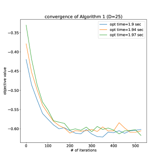
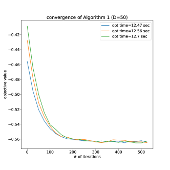
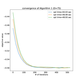
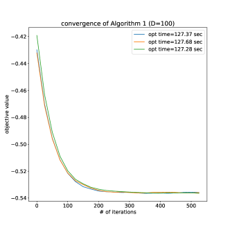
where $\ell(\alpha)=D^{-2}\sum_{i,j=1}^{D}(-)^{y_{i}\neq y_{j}}+\rho\|\alpha\|^{2}$ with $M_{r}\in{\mathbf{R}}_{+}^{D\times D}$ and $M_{r}=M_{r}^{T}$ ($r=1,\dots,R$), $Y\in\{1,\dots,N_{\rm labels}\}^{D}$ and $\rho>0$. Differently from usual sub-gradient descent algorithms, we do not check if the sub-gradient is a descent direction at each iteration. Such a check is based on the evaluation of the full-sample objective and, in our settings, requires solving the solution of an expansive all-pairs shortest path problem. To preserve the computational advantages of our approach, we use instead unchecked updates $\alpha^{(k+1)}=\alpha^{(k)}-\eta g^{(k)}$. Figure 1 shows that Algorithm 1 retains good convergence properties even with unchecked updates. Another option (not implemented here) would be to evaluate the objective on an arbitrary small validation data set extracted from the training samples. This would also allow a formal convergence proof and the definition of early stopping criteria. In Algorithm 1, we also implicitly assume that $\ell(\alpha^{(k)})$ is differentiable for all $k$ and use a simplified expression for its sub-gradients. If $\ell(\alpha)$ is differentiable in $\alpha$ it is possible to choose $\alpha=\alpha_{0}$ in (12) so that sub- and super-gradient coincide with the true gradient, provided by Theorem 2.6.

Algorithm 1 Soution of (28).

1:  Input: input metrics $\{M_{r}\}_{r=1}^{R}$, training labels $\{(y^{(d)}\}_{d=1}^{D}$, initialization $\alpha_{0}\in{\mathbf{R}}^{R}$, step size $\eta>0$, maximum number of iterations $k_{\rm max}\in{\mathbf{N}}_{+}$, regularization parameter $\rho>0$

2:  Initialize $\alpha^{(0)}=\alpha_{0}$

3:  while $k<k_{\rm max}$ do

4:     sample $(i,j)$ uniformly at random in $\{1,\dots,D\}\times\{1,\dots,D\}$

5:     let ${\cal G}={\cal G}(M_{\alpha^{k}})$

6:     let $\gamma_{*}=\min_{\gamma\in\Gamma_{ij}({\cal G})}\gamma^{T}{\rm softplus}(m_{\alpha}^{(k)})$

7:     for $r=1,\dots,R$ do

8:        let $[{\rm grad}^{(k)}]_{r}=D^{-2}(-)^{{\bf 1}_{y_{i}\neq y_{j}}}\gamma_{*}^{T}(\sigma([m_{\alpha^{(k)}}])\circ[m_{r}])$

9:     end for

10:     let $\alpha^{(k+1)}=\alpha^{(k)}-\eta({\rm grad}^{(k)}+2D^{-2}\rho\alpha^{(k)})$

11:  end while

12:  Output: $\alpha_{*}=\alpha^{(k_{\rm max})}$

Figure 1: Convergence of Algorithm 1 from slightly different initializations $\alpha=\frac{x}{\|x\|^{2}}$, with $x\sim{\cal N}(0,1)^{R}$ and $R=8$, and different size, $D$, of the input metrics $M_{r}$ ($r=1,\dots,R$, see Section 3.3 for more details). On the $y$-axis, we plot the value of $\ell(\alpha^{(k)})+\rho\|\alpha^{(k)}\|^{2}$ ($\rho=0.01$) evaluated on the training set. For all runs, we use the same data set, obtained from the MNIST database as explained in Section 3.3, and same learning parameters, $\eta=1$ and $k_{\max}=500$.

3 Experiments

3.1 Data

We use two real-world data sets: i) the MNIST data set, consisting of $N=70000$ images of grey-scale hand-written digits LeCun et al., (1998), and ii) the Citeseer dataset, containing $N=3327$ scientific papers and the corresponding citation network Sen et al., (2008).

MNIST data

We pre-process all grey-scale images in the MNIST data set and extract feature vectors of $d_{x}=784$ strictly positive entries. The images are labelled with integers $n=0,\dots,9$.

Citeseer data

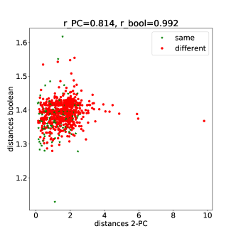
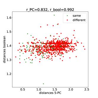
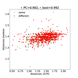
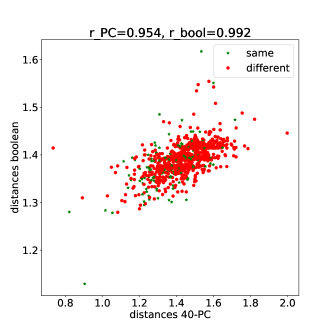
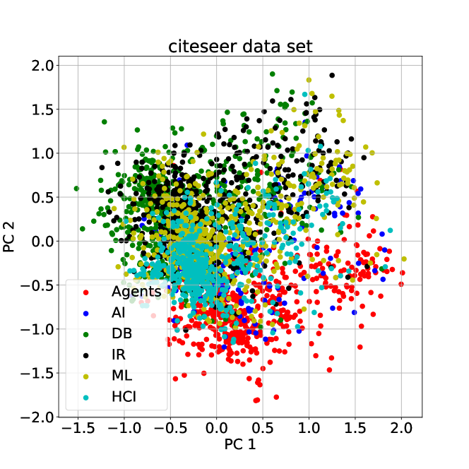
The Citeseer data set is a widely used as benchmark dataset for semi-supervised learning algorithms Sen et al., (2008); Kipf and Welling, (2016). The scientific papers are represented by bag-of-words feature vectors of dimensionality $d_{x}=3703$ and assigned according to their topic to 6 non-overlapping classes. The $d_{x}$-dimensional Boolean vectors are transformed into $40$-dimensional real vectors by projecting them onto the space of their first $40$ principal components. PCA projections can be shown to increase the clusters separation, but this is an optional step and our method would apply without changes with Boolean inputs. Figure 2 shows the predictive power of the Boolean data set, $X_{\rm bool}$, and a set of projected data sets, $X_{n\ {\rm PC}}$ ($n=2,5,10,40$). For each data set, $X_{\rm PC}=X_{n\ {\rm PC}}$, we have compared the ratio $r_{\rm data}=\frac{v_{\rm same}(X)}{v_{\rm different}(X)}$, where ${\rm data}\in\{PC,bool\}$ $v_{\rm same}=\sum_{(y,x),(y^{\prime},x^{\prime})\in X}{\bf 1}_{y=y^{\prime}}\|x-x^{\prime}\|^{2}$ and $v_{\rm diff}=\sum_{(y,x),(y^{\prime},x^{\prime})\in X}{\bf 1}_{y\neq y^{\prime}}\|x-x^{\prime}\|^{2}$ and $X=X_{\rm bool}$ and $X=X_{\rm PC}\}$. Figure 3 shows a two-dimensional (PCA) reduction of the data set. To make the calssification task harder, in Section 3.4 we use $X=X_{40\ {\rm PC}}$.

Figure 2: Cluster separation of the original (Boolean) word-embedding vectors and their projection on $n=2,5,10,40$ principal components. For each projected data set, $X_{n\ {\rm PC}}$ ($n=2,5,10,40$), and each paper pair (we randomly select 1000 paper pairs), we plot the distance between the corresponding word-embedding ($y$-axis) and PC vectors ($x$-axis). Different markers are used for pairs picked from the same cluster or different clusters. The total separation score, $r_{\rm data}$ ( ${\rm data}\in\{n\ {\rm PC},bool\}$) is the ratio between the average distance between papers in the same cluster, same, and between papers in different clusters, different.

Figure 3: Two-dimensional visualization of the Citeseer data set. Dimensional reduction is obtained by projecting on the first and second principal components. Different colors correspond to different topics.

3.2 Experiment 1: computational complexity (MNIST data)

To show the computational complexity gain associated with the intrinsic-metric approach we compare the proposed algorithm with a direct method, where metric constraints are imposed explicitly. We consider the optimization problem

$$\min_{\alpha\in{\mathbf{R}}^{R}} \ell(\alpha)=D^{-2}\|M_{\rm true}-M_{\alpha}\|^{2}$$ (30)

$${\rm s.t.} M_{\alpha}=\sum_{r=1}^{R}\alpha_{r}M_{r}\in{\cal M},$$ (31)

where $D$ is the number of images extracted from the MNIST data set and $M_{\rm true}$ and $M_{r}$ ($r=1,\dots,R$) are metrics of the selected data set defined by

$$\left[M_{\rm true}\right]_{ij} = \frac{\|x^{(i)}-x^{(j)}\|}{\sqrt{\|x^{(i)}\|\|x^{(j)}\|}},$$ (32)

$$\left[M_{r}\right]_{ij} = {\rm dist}_{\rm path}(i,j,G(A_{r})),$$ (33)

$$\left[A_{r}\right]_{ij} = {\bf 1}_{[M_{\rm true}]_{ij}<\xi_{r}},$$ (34)

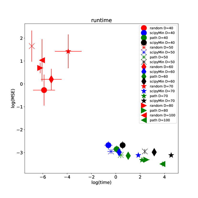
with $\xi_{r}=\bar{a}(\frac{1}{4}+(r-1)\frac{6}{4R})$, $\bar{a}=\frac{1}{D^{2}}\sum_{i,j=1}^{D}[M_{\rm true}]_{ij}$ and $R=8$. We compare the performance of the proposed method, path, with a state-of-the-art solver for constrained-quadratic programming, cvx. A regularization term, $\rho\|\alpha\|^{2}$ is added to objective minimized by cvx to make improve convergence speed. path is obtained by adapting Algorithm 1 to the least-squares objective $\ell(\alpha)$ defined in (30). The learning rate, $\eta$, is fixed for all $D$ and the optimization is stopped when $\ell^{(t+1)}<\ell^{(t)}(1+.0001)$, where $\ell^{(t)}=\ell(\alpha^{(t)})$ is the objective function defined in (30) evaluated on the training set and $\alpha^{(t)}$ is the value of the model parameter at the $t$th iteration. To assess the quality of the algorithms’ output, we consider a baseline, rand, where $\alpha_{\rm rand}=\frac{x}{\|x\|}$, with $x\sim{\cal N}(0,1)^{R}$. To facilitate the comparison and make the optimization more stable, we normalize $M_{r}$ in such a way $\|M_{r}\|=\|M_{\rm true}\|$ ($r=1,\dots,R$). For different sizes of the input metrics, $D=40,50,60,70,80,100$, Figure 4 shows the total runtime of the optimization versus $\ell(\alpha_{*})$, where $\alpha_{*}$ is the solution of (30) computed by the algorithms, or $\alpha_{*}=\alpha_{\rm rand}$. Runtime values associated with colored markers in Figure 4 do not include the computational time ($O(D^{3})$) for computing the constraints matrix, which is needed to implement the nonnegativity- and triangle- inequalities in cvx. The total time is indicated, on the same plot, by black markers. Different marker shapes in Figures 4 refer to different choices of $D$.

Figure 4: Runtime versus Mean Square Error at convergence. For cvx, values associated with colored markers do not include the computational cost of forming the constraints matrix, $A^{(D)}_{\rm constraints}\in\{-1,0,1\}^{O(D^{3})\times O(D^{2})}$, which is a required input of cvx. The corresponding total runtime, i.e. the optimization time plus the time needed to compute $A_{\rm constraints}^{(D)}$, is indicated by black markers and referred to by ${\bf cvx+extra}$ in the legend. Error bars represent standard deviations over 3 analogous experiments. Markers cvx D=80 and cvx D = 100 are not present because memory errors occurred while computing $A_{\rm constraints}^{(D)}$.

3.3 Experiment 2: feature space approximation (MNIST data)

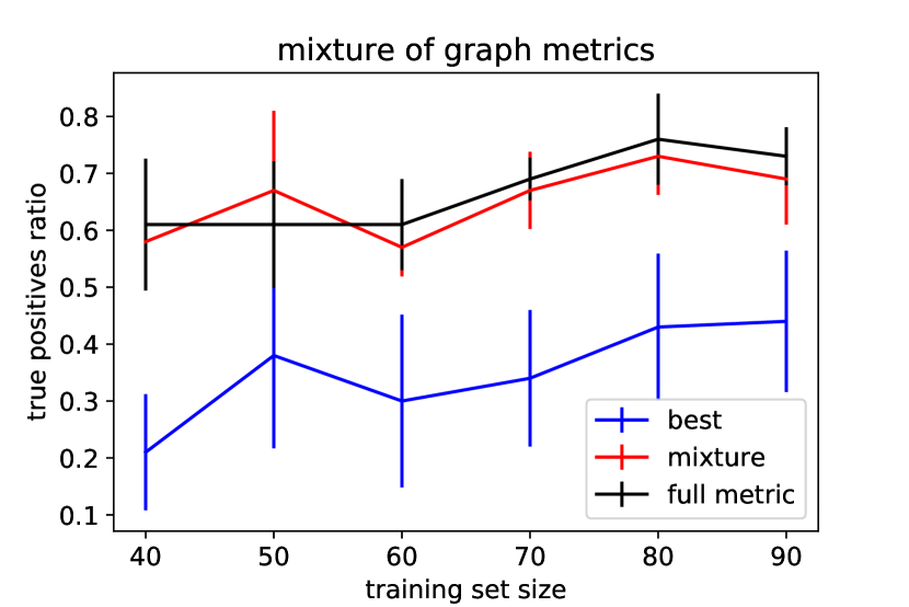
Main contribution of the proposed method (see Section 1.1) is the possibility of exploiting distinct non-Mahalanobis distance metrics simultaneously. In particular, this may allow one to combine the information coming from different graphs, each of them describing an independent aspects of a given system. In social networks applications, for example, different graphs can be associated with different kinds of relationship between users. The experiment shows how graph-related metrics can be merged to solve classification tasks. For simplicity, we the classification is performed through a $k=1$-Nearest Neighbor algorithm, where predicted labels for test set instances are the labels of their closest neighbour in the train set. We sample from the MNIST data base increasingly large train data sets, ${\cal D}^{(D)}_{\rm train}$ ($D=|{\cal D}^{(D)}_{\rm train}|=40,50,60,70,80,90$), and a test data set ${\cal D}_{\rm test}$ of size $D_{\rm test}=20$. All data sets contain $D$ grey-scale images and the corresponding labels, i.e. ${\cal D}_{\rm train}^{(D)}=\{(x^{(i)},y^{(i)}\}$ ($i=1,\dots,D$, idem ${\cal D}_{\rm test}$). For each $D$, we use the images in ${\cal D}_{\rm train}^{(D)}$ to compute the corresponding feature-space Euclidean metric, $M_{\rm true}\in{\mathbf{R}}^{D\times D}$, and a set of graph metrics $M_{r}$ ($r=1,\dots,R$), defined as in (32) with $x^{(i)}\in{\cal D}^{(D)}_{\rm train}$ ($i=1,\dots,D$). We assume that $M_{\rm true}$ is not available and train a linear combination of the graph metrics, $M_{\alpha}$, defined as (30). The possibly negative weight of the linear combination, $\alpha$, are the solution the linear metric-constrained optimization problem (28). The solution is obtained through the algorithm sketched in Algorithm 1. Finally, we use ${\cal D}_{\rm test}$ and a $k=1$ Nearest Neighbor algorithm to compare the predictive performance of the trained mixture, $M_{\alpha_{*}}$ and two other metrics, $M_{\rm true}$ and $M_{\rm best}$ (see below). More precisely, we let

$$y_{\rm predicted}^{(i^{\prime})}=y^{(i_{*})},\quad i_{*}={\rm arg}\min_{i=1,\dots,D}\bar{M}^{(i^{\prime})}_{(D+i^{\prime})i},$$ (35)

where $i^{\prime}=1,\dots,D_{\rm test}$, $\bar{M}\in\{\bar{M}^{(i^{\prime})}_{\alpha_{*}},\bar{M}^{(i^{\prime})}_{\rm true},\bar{M}^{(i^{\prime})}_{\rm best}\}$, $\bar{M}_{u}^{(i^{\prime})}\in{\mathbf{R}}^{(D+1)\times(D+1)}$ ($i^{\prime}=1,\dots,D$, $u=\alpha_{*},{\rm true},{\rm best}$) are defined as in (32) on the augmented data set ${\cal D}_{\rm train}^{(D)}\cup\{(x^{(i^{\prime})},y^{(i^{\prime})})\}$, $\alpha_{*}$ is the optimal solution of (28) and $\bar{M}^{(i^{\prime})}_{\rm best}=\bar{M}^{(i^{\prime})}_{r_{*}}$, with $r_{*}={\rm arg}\min_{r}\ell({\bf e}_{r})$. Figure 5 shows the performance of the three models versus the size of the training set.

Figure 5: Feature space approximation. Predictive power of a $(k=1)$ Nearest Neighbor algorithm based on a single graph metric (best), an optimized mixture of graph metrics (mixture)and the full feature-space Euclidean metric (full). Graph metrics are path-length distance metrics associated with graphs ${\cal G}(A_{\xi})$, where the adjacency metrics $A_{\xi}$ are defined by $[A_{\xi}]_{ij}={\bf 1}{[M_{\rm true}]_{i}j<\xi}$, for different choices of $\xi$. The single graph metric is obtained by solving (28) with simplex constraints on $\alpha$. Error bars represent standard deviations over 5 analogous experiments.

3.4 Experiment 3: semi-supervised learning (Citeseer data)

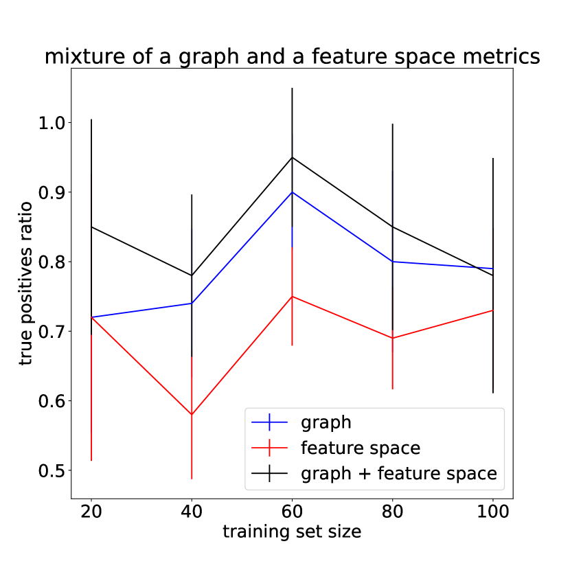
Most common applications of metric learning from structured data are to networks analysis. The problem is often cast as a semi-supervised learning problem, where the task is to predict a set of node labels, given their node attributes, a set of surrounding labelled nodes and the full edge structure of the graph. In those settings, it is natural to expect the prediction power of classification algorithms to be greatly improved if node and edge information can be effectively combined. We test the proposed algorithm on such a semi-supervised learning problem with $D_{\rm test}=20$ missing labels and training sets of different sizes. For both labelled and unlabelled nodes we have access to vectorized node attributes (the PC-projected word embedding of the Citeseer articles). The complete node- and edge-structure of the graph (the citation network) is also available during training and testing. In each experiment, we select sets of labelled articles from the Citeseer data base, ${\cal D}^{(D+D_{\rm test})}_{\rm train}$, ($D=20,40,60,80,100$) and extract the associated citation sub-graphs ${\cal G}^{(D+D_{\rm test})}_{\rm train}$. For all $D$, we use the citation sub-graphs, ${\cal G}^{(D+D_{\rm test})}_{\rm train}$, and the node features, $x^{(i)}\in{\cal D}^{(D+D_{\rm test})}_{\rm train}$ to compute two training metrics: $M_{\rm graph}\in{\mathbf{R}}^{(D+D_{\rm test})\times(D+D_{\rm test})}$, defined by $[M_{\rm graph}]_{ij}={\rm dist}_{\rm path}(i,j,{\cal G}^{(D)})$ ($i,j=1\dots,D+D_{\rm test}$), and $M_{\rm feature}\in{\mathbf{R}}^{(D+D_{\rm test})\times(D+D_{\rm test})}$, defined by $[M_{\rm feature}]_{ij}=\|x^{(i)}-x^{(j)}\|^{2}$. ($i,j=1\dots,D+D_{\rm test}$). We use the first $D$ (labelled) nodes to train a mixture model $M_{\alpha}=\alpha_{\rm graph}M_{\rm graph}+\alpha_{\rm feature}M_{\rm feature}$ and the remaining ‘unknown’ labels for testing. The predictive performance of a $(k=1)$ Nearest Neighbor algorithm based on $M_{\alpha}$ is compared with the same algorithm based on $M_{\rm graph}$ and $M_{\rm feature}$. Training is performed as described in Section 3.3 by solving (28) through Algorithm 1. Figure 6 shows the performance of the three models versus the size of the training set.

Figure 6: Semi-supervised learning. Predictive power of the $(k=1)$ Nearest Neighbor algorithm based on a single graph metric, graph, a single (Mahalonobis) feature-space metric, feature space, and an optimized mixture of the two, graph + feature space. The graph metric is a path-length distance metrics computed on the citation sub-graph associated with a subset of the Citeseer scientific papers. The feature-space metric is defined as the Euclidean distance between the corresponding (PC-projected) word-embedding vectors. Error bars represent standard deviations over 5 analogous experiments.

3.5 Results

Experiment 1

For small $D$, the performance of path (the proposed method) is equivalent to the performance of a state-of-the-art quadratic-optimization solver, cvx, in terms of accuracy and runtime. This s remarkable, as path is a general solver, i.e. it can be used for minimizing any (possibly non-convex) metric-constrained function, while cvx relies on the specific quadratic form of the objective. The proposed method can also handle cases where a direct optimization fails (for memory problems when $D>70$ on our machine). For large $D$, the quality of the output produced by path slightly increases, as it may be expected as the training set is larger, but computational times remain feasible. Performance improvements could be obtained by implementing a reduced-size early stopping test, where $\ell(\alpha)$ defined in (30) is replaced by $\ell_{\rm test}(\alpha)=\sum_{(i,j)\in{\cal I}_{\rm test}}[M_{\rm true}-M_{\alpha}]^{2}_{ij}$, with ${\cal I}_{\rm test}$ being a small set of index pairs. Tuning the learning parameters for each specific $D$ can also reduce the computational time and increase the output quality.

Experiment 2

The reported performance of mixture shows that a combination of graph metrics can be statistically equivalent to a full feature-space metric. It is important to stress here that goal of our simulation was not to show that graph-based metrics can be better than feature-space metrics. In our settings, this would make little sense as all graph-based metrics are obtained by cutting out some of the information contained in the full feature-space metric, $M_{\rm true}$. The feature-space metric should be looked at as a ‘ground truth’ model, which can be naturally expected to achieve the best performance. What we want to show, instead, is that the proposed algorithm is actually able to combine the information encoded by distinct graph structures in a consistent way. This is underlined by the statistically robust performance gap between best and mixture.

Experiment 3

Results suggest that merging information from a vector-valued feature space and given graph structures is often profitable. As in the previous experiments, we have considered minimal settings for clarity reasons. The overall predictive performance of the model would obviously be increased if more feature-space and graph-based metrics are added to the mixture. For example, $M_{\rm feature}$ could be replaced by a set of pre-optimized Mahalanobis metrics (obtained through usual metric-learning methods on the same data set) and the path-length metric by a set of different graph-based dissimilarity matrices. As expected, the benefits of a combined approach are more remarkable when the size of the training data set is small and meaningful independent information can be extracted from both $M_{\rm feature}$ and $M_{\rm graph}$. The slight performance’s drop of mixture for increasing sizes of the training data set maybe due to i) a certain redundancy between the two metrics or ii) the fact that the algorithm has not completely converged. Convergence problems for large values of $D$ probably arise because we run Algorithm 1 with a single set of optimization parameters for all values of $D$.

4 Discussion

The main contribution of this work can be summarized as follows. We propose a new algorithm for optimizing a general objective under metric constraints and provide theoretical arguments for analyzing the algorithm’s convergence in a specific but useful case. We describe how the scheme can be used in network-based application for combining heterogeneous information extracted from the graph structure and the feature space associated with the node attributes. We run simple experiments to show that the predictive power of simple classification algorithm is indeed boosted by merging a set of Mahalanobis and non-Mahalanobis metrics.

Possible future extensions of this work go in three directions.

Large scale approximation

As the computational bottleneck of the algorithm is the computation of single-pair shortest paths, the overall speed of the algorithm may be increased by considering large-scale approximations of the metrics or a faster versions of the Dijkstra algorithm.

Mixture of local metrics

It has been shown that local metrics may outperform global ones in different tasks. The proposed approach can be used to define data-dependent, i.e. local, linear combination of pre-learned local metrics. This would be an interesting but challenging application, as the objective function would become nonlinear in the parameters.

Nonlinear combination of metrics

Since the proposed method does not require the linearity or convexity of the metric model possibly nonlinear and more flexible functions of the input matrices may be explored, e.g. by letting $M_{\alpha}=\phi_{\alpha}(\{M_{r}\})$, where $\phi_{\alpha}$ is a metric-projected neural network.

References

- Bandelt and Chepoi, (2008) Bandelt, H.-J. and Chepoi, V. (2008). Metric graph theory and geometry: a survey. Contemporary Mathematics, 453:49–86.
- Basri et al., (1998) Basri, R., Costa, L., Geiger, D., and Jacobs, D. (1998). Determining the similarity of deformable shapes. Vision Research, 38(15-16):2365–2385.
- Batra et al., (2008) Batra, D., Sukthankar, R., and Chen, T. (2008). Semi-supervised clustering via learnt codeword distances. In BMVC, pages 1–10. Citeseer.
- Bellet et al., (2013) Bellet, A., Habrard, A., and Sebban, M. (2013). A survey on metric learning for feature vectors and structured data. arXiv preprint arXiv:1306.6709.
- Bilenko et al., (2004) Bilenko, M., Basu, S., and Mooney, R. J. (2004). Integrating constraints and metric learning in semi-supervised clustering. In Proceedings of the twenty-first international conference on Machine learning, page 11. ACM.
- Boyd et al., (2003) Boyd, S., Xiao, L., and Mutapcic, A. (2003). Subgradient methods. lecture notes of EE392o, Stanford University, Autumn Quarter, 2004:2004–2005.
- Brickell et al., (2008) Brickell, J., Dhillon, I. S., Sra, S., and Tropp, J. A. (2008). The metric nearness problem. SIAM Journal on Matrix Analysis and Applications, 30(1):375–396.
- Bridson and Haefliger, (2013) Bridson, M. R. and Haefliger, A. (2013). Metric spaces of non-positive curvature, volume 319. Springer Science & Business Media.
- Bronstein et al., (2007) Bronstein, A. M., Bronstein, M. M., and Kimmel, R. (2007). Rock, paper, and scissors: extrinsic vs. intrinsic similarity of non-rigid shapes. In Computer Vision, 2007. ICCV 2007. IEEE 11th International Conference on, pages 1–6. IEEE.
- Buckley and Harary, (1990) Buckley, F. and Harary, F. (1990). Distance in graphs. Addison-Wesley.
- Burago et al., (2001) Burago, D., Burago, Y., and Ivanov, S. A. (2001). A course in metric geometry, volume 33. American Mathematical Soc.
- Burdet and Johnson, (1975) Burdet, C.-A. and Johnson, E. L. (1975). A subadditive approach to solve linear integer programs. Annals of Discrete Mathematics, 1:117–144.
- Cox and Cox, (2000) Cox, T. F. and Cox, M. A. (2000). Multidimensional scaling. Chapman and hall/CRC.
- Diestel, (2018) Diestel, R. (2018). Graph theory. Springer Publishing Company, Incorporated.
- Dykstra, (1983) Dykstra, R. L. (1983). An algorithm for restricted least squares regression. Journal of the American Statistical Association, 78(384):837–842.
- Fei-Fei and Perona, (2005) Fei-Fei, L. and Perona, P. (2005). A bayesian hierarchical model for learning natural scene categories. In 2005 IEEE Computer Society Conference on Computer Vision and Pattern Recognition (CVPR’05), volume 2, pages 524–531. IEEE.
- Hanson and Martin, (1990) Hanson, W. and Martin, R. K. (1990). Optimal bundle pricing. Management Science, 36(2):155–174.
- Hauberg et al., (2012) Hauberg, S., Freifeld, O., and Black, M. J. (2012). A geometric take on metric learning. In Advances in Neural Information Processing Systems, pages 2024–2032.
- Hoi et al., (2006) Hoi, S. C., Liu, W., Lyu, M. R., and Ma, W.-Y. (2006). Learning distance metrics with contextual constraints for image retrieval. In Computer vision and pattern recognition, 2006 IEEE computer society conference on, volume 2, pages 2072–2078. IEEE.
- Igelmund and Radermacher, (1983) Igelmund, G. and Radermacher, F. J. (1983). Preselective strategies for the optimization of stochastic project networks under resource constraints. Networks, 13(1):1–28.
- Keller, (2015) Keller, M. (2015). Intrinsic metrics on graphs: a survey. In Mathematical technology of networks, pages 81–119. Springer.
- Kipf and Welling, (2016) Kipf, T. N. and Welling, M. (2016). Semi-supervised classification with graph convolutional networks. arXiv preprint arXiv:1609.02907.
- Kulis et al., (2013) Kulis, B. et al. (2013). Metric learning: A survey. Foundations and Trends® in Machine Learning, 5(4):287–364.
- Lanckriet et al., (2004) Lanckriet, G. R., Cristianini, N., Bartlett, P., Ghaoui, L. E., and Jordan, M. I. (2004). Learning the kernel matrix with semidefinite programming. Journal of Machine learning research, 5(Jan):27–72.
- Laub and MÞller, (2004) Laub, J. and MÞller, K.-R. (2004). Feature discovery in non-metric pairwise data. Journal of Machine Learning Research, 5(Jul):801–818.
- LeCun et al., (1998) LeCun, Y., Bottou, L., Bengio, Y., and Haffner, P. (1998). Gradient-based learning applied to document recognition. Proceedings of the IEEE, 86(11):2278–2324.
- Lodhi et al., (2002) Lodhi, H., Saunders, C., Shawe-Taylor, J., Cristianini, N., and Watkins, C. (2002). Text classification using string kernels. Journal of Machine Learning Research, 2(Feb):419–444.
- Mémoli, (2011) Mémoli, F. (2011). Metric structures on datasets: stability and classification of algorithms. In International Conference on Computer Analysis of Images and Patterns, pages 1–33. Springer.
- Mennucci, (2004) Mennucci, A. (2004). On asymmetric distances. URL http://cvgmt. sns. it/papers/and04/. 2nd version.
- Pillutla et al., (2018) Pillutla, V. K., Roulet, V., Kakade, S. M., and Harchaoui, Z. (2018). A smoother way to train structured prediction models. In Advances in Neural Information Processing Systems, pages 4766–4778.
- Roth et al., (2003) Roth, V., Laub, J., Müller, K.-R., and Buhmann, J. M. (2003). Going metric: Denoising pairwise data. In Advances in Neural Information Processing Systems, pages 841–848.
- Rudin et al., (1964) Rudin, W. et al. (1964). Principles of mathematical analysis, volume 3. McGraw-hill New York.
- Salton et al., (1975) Salton, G., Wong, A., and Yang, C.-S. (1975). A vector space model for automatic indexing. Communications of the ACM, 18(11):613–620.
- Sen et al., (2008) Sen, P., Namata, G., Bilgic, M., Getoor, L., Galligher, B., and Eliassi-Rad, T. (2008). Collective classification in network data. AI magazine, 29(3):93–93.
- Shaw et al., (2011) Shaw, B., Huang, B., and Jebara, T. (2011). Learning a distance metric from a network. In Advances in Neural Information Processing Systems, pages 1899–1907.
- Shaw and Jebara, (2009) Shaw, B. and Jebara, T. (2009). Structure preserving embedding. In Proceedings of the 26th Annual International Conference on Machine Learning, pages 937–944.
- Shi et al., (2014) Shi, Y., Bellet, A., and Sha, F. (2014). Sparse compositional metric learning. In Twenty-Eighth AAAI Conference on Artificial Intelligence.
- Shor, (2012) Shor, N. Z. (2012). Minimization methods for non-differentiable functions, volume 3. Springer Science & Business Media.
- Shor, (2013) Shor, N. Z. (2013). Nondifferentiable optimization and polynomial problems, volume 24. Springer Science & Business Media.
- Veldt et al., (2018) Veldt, N., Gleich, D., Wirth, A., and Saunderson, J. (2018). A projection method for metric-constrained optimization. arXiv preprint arXiv:1806.01678.
- Weinberger and Saul, (2009) Weinberger, K. Q. and Saul, L. K. (2009). Distance metric learning for large margin nearest neighbor classification. Journal of Machine Learning Research, 10(Feb):207–244.
- West et al., (2001) West, D. B. et al. (2001). Introduction to graph theory, volume 2. Prentice hall Upper Saddle River.
- Williams and Williams, (2018) Williams, V. V. and Williams, R. R. (2018). Subcubic equivalences between path, matrix, and triangle problems. Journal of the ACM (JACM), 65(5):27.
- Xing et al., (2003) Xing, E. P., Jordan, M. I., Russell, S. J., and Ng, A. Y. (2003). Distance metric learning with application to clustering with side-information. In Advances in neural information processing systems, pages 521–528.
- Yu et al., (2006) Yu, J., Tian, Q., Amores, J., and Sebe, N. (2006). Toward robust distance metric analysis for similarity estimation. In Computer Vision and Pattern Recognition, 2006 IEEE Computer Society Conference on, volume 1, pages 316–322. IEEE.
- Zaustinsky, (1959) Zaustinsky, E. M. (1959). Spaces with non-symmetric distance, volume 34. American Mathematical Soc.