Age of Information with Gilbert-Elliot
Servers and Samplers††thanks: This work was supported by NSF Grants CCF 17-13977 and ECCS 18-07348.
Abstract
We study age of information in a status updating system that consists of a single sampler, i.e., source node, that sends time-sensitive status updates to a single monitor node through a server node. We first consider a Gilbert-Elliot service profile at the server node. In this model, service times at the server node follow a finite state Markov chain with two states: bad state and good state where the server is faster in state . We determine the time average age experienced by the monitor node and characterize the age-optimal state transition matrix with and without an average cost constraint on the service operation. Next, we consider a Gilbert-Elliot sampling profile at the source. In this model, the interarrival times follow a finite state Markov chain with two states: bad state and good state where samples are more frequent in state . We find the time average age experienced by the monitor node and characterize the age-optimal state transition matrix .
I Introduction
Age of information (AoI) is a network performance metric which has been proposed to assess the timeliness in real-time status updating systems. Such systems include sensor networks, vehicular networks, and emergency alarm systems. In all these systems, time-critical data generated by the source node(s) are sent to the interested monitor node(s). Here, the update packets are time-critical since the information loses its value as it becomes stale. Thus, overall freshness of the information is desired which motivates the study of age of information in communication networks with various foci, e.g., queueing theory [1, 2, 3, 4, 5, 6, 7, 8, 9, 10, 11, 12, 13], scheduling and energy harvesting [14, 15, 16, 17, 18, 19, 20, 21, 22, 23, 24, 25, 26, 27, 28, 29], and caching and coding [30, 31, 32, 33, 34, 35, 36, 37, 38, 39].
In all these works, there is an underlying i.i.d. structure in the system. The service times and packet interarrivals are i.i.d. processes and the focus is on analyzing and optimizing the resulting age of information. There may be scenarios in which these processes are correlated over time or over different status update packets. Reference [40] models transmission times as a stationary and ergodic Markov chain to analyze the effect of the temporal correlation between transmission times on age-optimal scheduling. References [41, 42] study information freshness over Markovian channels. Specifically, reference [41] models the channel using a Gilbert-Elliot model and introduces the concept of channel information age. This metric is used to express the utility and analyze the effect of aging on the probability of error in estimating the channel state. Reference [43] studies the freshness over a network with a Markov source and proposes an effective age metric which captures estimation error as well as timeliness. Reference [44] studies age of information with a two-state Markov modulated service process and characterizes the average age for an FCFS operation under infinite and zero buffer size settings.

In this work, we consider a status updating system in which there is a single sampler which takes samples from an observed phenomenon and sends them to an interested monitor node in the form of status update packets through a single server node (see Fig. 1). We study age of information with Gilbert-Elliot servers and samplers under blocking packet management policy at the server node. We first analyze the case in which the service times follow a finite state Markov chain with two states: bad state and good state such that in state , the service performance is faster than that in state . The motivation for studying this kind of a service profile comes from the measurements over Amazon EC2 clusters which show high variability in computing speeds of the servers over time [45]. These measurements indicate that when a server is in a certain state it tends to stay in that state in the next rounds of the computation which implies a dependence in service times over time. In addition, [46] shows that the channel quality and reliability in cooperative driving follows a Markov-modulated process which depends on the number of interfering vehicles thereby affecting the service performance. Further, in sensor networking applications, energy constraints on servers may prevent them from operating in faster states all the time, and may force them to switch between faster and slower states.
We derive the time average age under this Markovian service profile and characterize the age-optimal state transition matrix of the underlying Markov chain first without considering any constraints on the operation of the system. Next, we consider a more realistic scenario in which each state has an operational cost and the system is subject to an overall budget.
Next, we consider the case in which the sampler, i.e, the source node, follows a Gilbert-Elliot model based operation. The sampler takes samples based on a two-state Markov chain, as in Fig. 1. When in state , it samples the observed phenomenon more frequently whereas in state , samples are taken more sparsely. Thus, under this operation, interarrivals to the server node are no longer i.i.d. but follow a two-state Markov chain. This non i.i.d. sampling operation is particularly relevant when the sampler’s operation cost is considered as the sampler may not be able to afford taking frequent samples all the time and may switch to a low-cost operation to save energy. Further, the sampler may choose to sample the process more often when the observed process varies above a certain threshold or varies too fast. We characterize the average age under such Gilbert-Elliot sampling and find the age-optimal state transition matrix .
II System Model and Age Metric
We consider a communication system (see Fig. 1), where there is a single sampler that takes samples from an observed phenomenon at random and immediately transmits these samples to a monitor node through a single server node in the form of status update packets. The server node implements a blocking policy in which an arriving update packet goes directly into service only if the server is idle. Update packets arriving when the server node is busy are discarded.
Unlike most of the literature, we consider non i.i.d. service and interarrival profiles. Here, we use a simple Gilbert-Elliot model to introduce a non i.i.d. structure to the system. We consider two scenarios: Gilbert-Elliot service times and i.i.d. interarrival times; and i.i.d. service times and Gilbert-Elliot interarrival times.
When the server follows a Gilbert-Elliot model, service times follow a two state Markov chain with states bad () and good () such that in state , the server node is slower and the service takes longer than the service in state . We model the service times with exponential random variables with rate in state and with rate in state where as in [44]. In this case, we model the update arrivals at the server node as a Poisson process with rate . We adopt an event-triggered Markov chain in which the state change only occurs when a new packet enters service. Thus, during the service of an update packet, service performance remains the same. The transition probability from state to state is and the transition probability from state to state is where and (see Fig. 1). State transition matrix of this Markov chain is
| (1) |
We note that this Markov chain is irreducible, aperiodic, and positive recurrent. Thus, service times constitute an ergodic Markov chain with a stationary distribution,
| (2) |
where is the service time of a packet that enters service.
When the sampler follows a Gilbert-Elliot model, this time, update interarrivals at the server node constitute a Markov chain with the state transition matrix in (1) where in state interarrival times are exponential random variables with rate and in state interarrival times are exponential random variables with rate where to reflect the increased sampling frequency in state . The Markov chain is again event-triggered such that the sampler’s state changes whenever an update packet enters service at the server node.
To quantify the timeliness in the system, we use the age of information metric. At time age at the monitor node is the random process where is the time-stamp of the most recent update at the destination node. The metric we use, time averaged age, is given by
| (3) |
where is the instantaneous age at the monitor node.
In the next section, we derive an average age expression for the cases of Gilbert-Elliot servers and samplers.
III Average Age Analysis
The sampler generates status update packets and immediately sends them through a delay-free link to the server node. Since a blocking policy is implemented, only the packets that find the server idle go into service. We denote such packets that enter service at the server node as successful packets. Let denote the time at which the th successful update packet is generated at the sampler. Since newly generated packets are assumed to be instantaneously available to the server node, also marks the time at which the th successful update packet arrives at the server node. Random variable denotes the update cycle at the server node, the time in between two successful arrivals, where .
Update cycle consists of service time and idle waiting time as the server needs to wait for the next arrival upon an update delivery to the monitor node such that
| (4) |
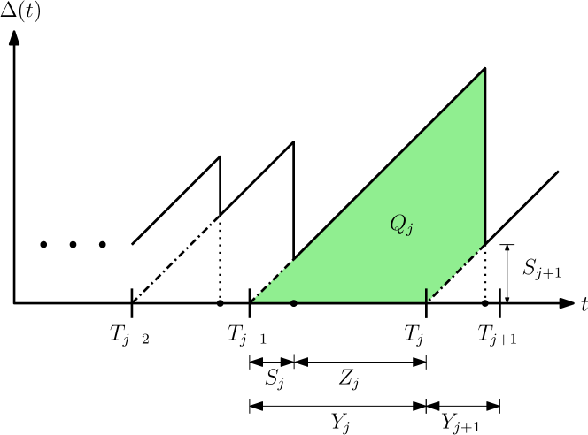
We note that and are mutually independent as the arrival and service processes are independent. Sample age evolution at the destination node is given in Fig. 2. Here, denotes the area under the instantaneous age curve in update cycle and denotes the length of the th update cycle as defined earlier. The metric we use, long term average age, is the average area under the age curve which is given [1, 3] by
| (5) |
In the next two subsections, we find the average age for Gilbert-Elliot service times and interarrival times, respectively.
III-A Gilbert-Elliot Service Times and I.i.d. Interarrival Times
Status update packets arrive at the server node as a Poisson process with rate . Thus, update packet interarrivals at the server node are i.i.d. exponential random variables with rate . Due to the memoryless property of the update arrivals at the server node, is also exponentially distributed with rate . Service times follow a two-state Markov chain. Thus, two consecutive service times are dependent through the state transition matrix given in (1).
Conditioned on and , the th update cycle and the area under the age curve in this cycle are characterized by
| (6) |
We note that when the service times and interarrival times are i.i.d., we have a renewal process with inter-renewal time equal to the update cycle . However, in our model, update cycles do not form an i.i.d. sequence unlike the prior models considered in the literature. Rather, each is characterized as in (6) depending on the state of the service time in update cycles and . Since the underlying Markov chain is stationary and ergodic, we have over all update cycles and (5) reduces to
| (7) |
where the first equality follows from [40, Appendix A] and the second equality follows from the law of total probability where we define and . From this, along with Fig. 2, we get
| (8) | ||||
| (9) |
where
| (10) | |||
| (11) |
In addition, from (6) we have,
| (12) | |||
| (13) |
since as defined earlier.
III-B Gilbert-Elliot Interarrival Times and I.i.d. Service Times
Service times at the server node are i.i.d. exponential random variables with rate whereas the interarrival times follow a two-state Markov chain characterized by the state transition matrix in (1). State changes occur upon successful entry to the server node. Let denote the waiting time until the next arrival when the interarrival state is , and let denote the waiting time when the interarrival state is . Thus,
| (15) |
Here, similar stationarity and ergodicity arguments apply and the average age is again given by
| (16) |
By inspecting Fig. 2, we find
| (17) | ||||
| (18) |
In addition, we have,
| (19) | |||
| (20) |
by using (15) and the fact that .
Substituting (17)-(20) in (16) yields the average age expression under Gilbert-Elliot interarrival times and i.i.d. service times. We note that both the numerator and denominator of (16) are linear in and .
So far, we derived average age expressions for Gilbert-Elliot servers and samplers for a given state transition matrix . We optimize this matrix in the next section to achieve minimum average age at the monitor node in both scenarios.
IV Age-Optimal Transition Matrix
In what follows we characterize the age-optimal state transition matrix for Gilbert-Elliot service times and Gilbert-Elliot interarrival times.
IV-A Gilbert-Elliot Service Times and I.i.d. Interarrival Times
In Section III-A the average age expression (7) for given state transition matrix under Gilbert-Elliot service times is derived. Next two lemmas characterize the behavior of (7) with respect to the state transition probabilities and .
Lemma 1
Under Gilbert-Elliot service times, the average age in (7) monotonically decreases in .
Proof: To prove the lemma, we take the derivative of (7) with respect to and show that it is negative. The numerator of the derivative of (7) is
| (21) |
In (21), the last term is already negative as as stated in Section II. Thus, we need to show that . This is indeed true for exponential interarrival times with rate and exponential service times with rate in state and with rate in state where . With this, the result follows.
Thus, as increases, a better age performance is achieved at the monitor node. This is an intuitive result as larger indicates that the service state spends more time in the good state as implied by (2). We note that this result does not depend on and is valid for any .
Lemma 2
Under Gilbert-Elliot service times, the average age in (7) monotonically increases in .
IV-B Gilbert-Elliot Interarrival Times and I.i.d. Service Times
In Section III-B the average age expression (16) for given state transition matrix under Gilbert-Elliot interarrival times is derived. Next two lemmas, which follow similar to Lemmas 1 and 2, characterize the behavior of (16) with respect to the state transition probabilities and .
Lemma 3
Under Gilbert-Elliot interarrival times, the average age in (16) monotonically decreases in .
Thus, as increases, a better age performance is achieved at the monitor node as in Gilbert-Elliot service times scenario.
Lemma 4
Under Gilbert-Elliot interarrival times, the average age in (16) monotonically increases in .
Thus, as decreases, a better age performance is achieved at the monitor node as in Gilbert-Elliot service times scenario.
From Lemmas 3 and 4, we observe that, to achieve the minimum average age under Gilbert-Elliot interarrival times, we need to maximize the time spent in state . Although more frequent sampling may overwhelm the network and incur higher age in FCFS queueing systems as shown in [1], in our model, since a dropping policy is implemented, more frequent sampling is desirable to obtain lower average age.
In the next section, we find the age-optimal state transition matrix when there is an average cost constraint.
V Age-Optimal Transition Matrix under Average Cost Constraint
In Section IV, the age optimization is over all possible and pairs, i.e., and we showed that as and , the minimum age is achieved in both scenarios. However, when there is a constraint on the operation of the system, all of region may not be feasible. To explore the age-optimal state transition probabilities in such a scenario, here, we consider a constraint on the average cost which may correspond possibly to limited energy budget for the system. Let and denote the cost of operating in state and state , respectively, where as faster operation requires higher cost (e.g., more energy). When the overall budget is units, we need to satisfy
| (22) |
Then, the problem to solve becomes,
| s.t. | (23) |
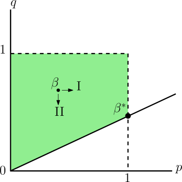
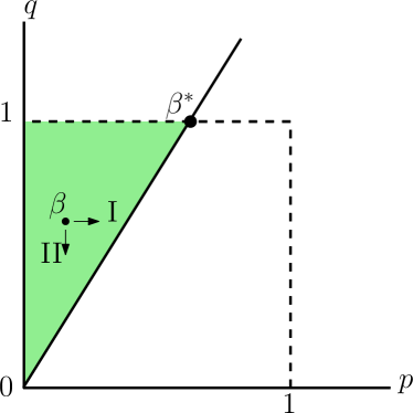
where expectations are as in (8)-(13) for Gilbert-Elliot service times and as in (17)-(20) for Gilbert-Elliot interarrival times and the constraint follows from (22). The trivial case is when for which the feasible region is and the results from Section IV apply. Thus, in this section, we consider for which the feasible set is shown in Fig. 3. Next, we show that the constraint in (V) needs to be satisfied with equality.
Lemma 5
Age-optimal pair satisfies the constraint in (V) with equality, i.e., .
Proof: Given a point in the feasible set as shown in Fig. 3, a lower average age can be obtained as we move along direction I to increase or along direction II to decrease as shown in Lemmas 1 and 2 under Gilbert-Elliot service times and in Lemmas 3 and 4 under Gilbert-Elliot interarrival times. Thus, no point that is not along the line can be optimal as we can achieve a lower average age by moving towards this line.
Thus, the age-optimal pair is such that where . With this, the problem in (V) reduces to a minimization over probability only. That is, the objective function in (V) becomes
| (24) |
where is fixed. Next, we solve this problem for Gilbert-Elliot service times and Gilbert-Elliot interarrival times and find the age-optimal pair that minimizes the average age.
V-A Gilbert-Elliot Service Times and I.i.d. Interarrival Times
We note that, under Gilbert-Elliot service times, the denominator of (24) does not depend on whereas the numerator depends on linearly. One can show that (24) is a decreasing function of with an argument similar to that of Lemma 1. Thus, provided that , the age-optimal transition matrix under average cost constraint is such that and which is the point in Fig. 3(a). This result is intuitive as it maximizes the transition probability from state to state and spends fraction of time in state to satisfy the budget requirement. For example, when , and we find and the optimal selection is and .
Otherwise, when , the age-optimal selection is and which is the point in Fig. 3(b). This result tells us that in the age minimizing operation the transition probability from state to state approaches since the transition probability from state to state is already limited by . For example, when , and we find and the age-optimal selection is and .
V-B Gilbert-Elliot Interarrival Times and I.i.d. Service Times
We note that, under Gilbert-Elliot interarrival times, both the numerator and the denominator of (24) do not depend on . Thus, any and corresponding for the given yields the same average age. In other words, as long as we operate in in Fig. 3, i.e., satisfy (22) with equality, we obtain the optimal average age since (16) depends on and only through the stationary probabilities of the states given in (2) as expectations in (17)-(20) do not depend on and .
VI Numerical Results
In this section, we provide simple numerical results to validate our theoretical results for a system with arbitrary exponential interarrival and service times.
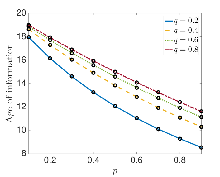
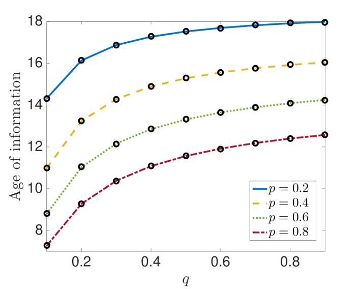
We consider Gilbert-Elliot service times and take which is the rate of Poisson arrivals to the server node. We model the service times with an exponential random variable with rate in state and with rate in state . In Figs. 4 and 5, we plot the average age of information under Gilbert-Elliot service times as a function of the state transition probabilities and , respectively. In both of the figures, we plot simulation results, marked with symbol, along with results obtained from (7) and observe that the results match. Fig. 4 shows that the average age decreases monotonically as probability gets larger as shown in Lemma 1. Here, we also note that as gets lower for a fixed value, we achieve a lower average age as discussed earlier in Section IV. Fig. 5 shows that the age of information increases monotonically as probability increases. We also observe that for a fixed value, the best age is obtained when the probability is the largest. When the server node only operates in the good state , we find that . We observe that this value is lower than the age values in Figs. 4 and 5 as the server does not slow down by switching to the bad state . Similarly, if the server node only operates in the bad state , we find that which is strictly larger than the age values shown in Figs. 4 and 5. Thus, in this case, the server node benefits from switching to the good state .
VII Conclusions
In this work, we considered an information update system in which status update packets are generated by a sampler and sent to a monitor node through a server node. We considered two scenarios: Gilbert-Elliot service times and i.i.d. interarrival times; and Gilbert-Elliot interarrival times and i.i.d. service times. In these scenarios, either the server or the sampler follows a two-state Markov chain with the good state and the bad state where the operation is faster in state . We determined the average age at the monitor node for both scenarios and characterized the age-optimal state transition matrix for the underlying Markov chain with and without an average cost constraint on the operation of the system.
References
- [1] S. K. Kaul, R. D. Yates, and M. Gruteser. Real-time status: How often should one update? In IEEE Infocom, March 2012.
- [2] M. Costa, M. Codreanu, and A. Ephremides. On the age of information in status update systems with packet management. IEEE Transactions on Information Theory, 62(4):1897–1910, April 2016.
- [3] R. D. Yates and S. K. Kaul. Real-time status updating: Multiple sources. In IEEE ISIT, July 2012.
- [4] E. Najm, R. D. Yates, and E. Soljanin. Status updates through M/G/1/1 queues with HARQ. In IEEE ISIT, June 2017.
- [5] Y. Inoue. Analysis of the age of information with packet deadline and infinite buffer capacity. In IEEE ISIT, June 2018.
- [6] A. Soysal and S. Ulukus. Age of information in G/G/1/1 systems. In Asilomar Conference, November 2019.
- [7] A. Soysal and S. Ulukus. Age of information in G/G/1/1 systems: Age expressions, bounds, special cases, and optimization. May 2019. Available on arXiv: 1905.13743.
- [8] J. Zhong, E. Soljanin, and R. D. Yates. Status updates through multicast networks. In Allerton Conference, October 2017.
- [9] B. Buyukates, A. Soysal, and S. Ulukus. Age of information in two-hop multicast networks. In Asilomar Conference, October 2018.
- [10] B. Buyukates, A. Soysal, and S. Ulukus. Age of information in multicast networks with multiple update streams. In Asilomar Conference, November 2019.
- [11] B. Buyukates, A. Soysal, and S. Ulukus. Age of information in multihop multicast networks. Journal of Communications and Networks, special issue on Age of Information, 21(3):256–267, July 2019.
- [12] A. Maatouk, M. Assaad, and A. Ephremides. Age of information with prioritized streams: When to buffer preempted packets? January 2019. Available on arXiv: 1901.05871.
- [13] V. Tripathi, R. Talak, and E. Modiano. Age of information for discrete time queues. January 2019. Available on arXiv: 1901.10463.
- [14] Y. Hsu, E. Modiano, and L. Duan. Age of information: Design and analysis of optimal scheduling algorithms. In IEEE ISIT, June 2017.
- [15] B. Zhou and W. Saad. Optimal sampling and updating for minimizing age of information in the internet of things. In IEEE Globecom, December 2018.
- [16] M. Bastopcu and S. Ulukus. Minimizing age of information with soft updates. Journal of Communications and Networks, special issue on Age of Information, 21(3):233–243, July 2019.
- [17] M. Bastopcu and S. Ulukus. Age of information for updates with distortion. In IEEE ITW, August 2019.
- [18] M. Bastopcu and S. Ulukus. Age of information for updates with distortion: Constant and age-dependent distortion constraints. December 2019. Available on arXiv: 1912.13493.
- [19] M. Bastopcu and S. Ulukus. Who should Google Scholar update more often? January 2020. Available on arXiv: 2001.11500.
- [20] S. Ioannidis, A. Chaintreau, and L. Massoulie. Optimal and scalable distribution of content updates over a mobile social network. In IEEE Infocom, April 2009.
- [21] B. Buyukates, A. Soysal, and S. Ulukus. Age of information scaling in large networks. In IEEE ICC, May 2019.
- [22] B. Buyukates, A. Soysal, and S. Ulukus. Age of information scaling in large networks with hierarchical cooperation. In IEEE Globecom, December 2019.
- [23] B. T. Bacinoglu, E. T. Ceran, and E. Uysal-Biyikoglu. Age of information under energy replenishment constraints. In UCSD ITA, February 2015.
- [24] X. Wu, J. Yang, and J. Wu. Optimal status update for age of information minimization with an energy harvesting source. IEEE Transactions on Green Communications and Networking, 2(1):193–204, March 2018.
- [25] A. Arafa, J. Yang, S. Ulukus, and H. V. Poor. Age-minimal online policies for energy harvesting sensors with incremental battery recharges. In UCSD ITA, February 2018.
- [26] A. Arafa, J. Yang, S. Ulukus, and H. V. Poor. Online timely status updates with erasures for energy harvesting sensors. In Allerton Conference, October 2018.
- [27] S. Farazi, A. G. Klein, and D. R. Brown III. Average age of information for status update systems with an energy harvesting server. In IEEE Infocom, April 2018.
- [28] A. Baknina, O. Ozel, J. Yang, S. Ulukus, and A. Yener. Sending information through status updates. In IEEE ISIT, June 2018.
- [29] S. Leng and A. Yener. Minimizing age of information for an energy harvesting cognitive radio. In IEEE WCNC, April 2019.
- [30] R. D. Yates, P. Ciblat, A. Yener, and M. Wigger. Age-optimal constrained cache updating. In IEEE ISIT, June 2017.
- [31] C. Kam, S. Kompella, G. D. Nguyen, J. Wieselthier, and A. Ephremides. Information freshness and popularity in mobile caching. In IEEE ISIT, June 2017.
- [32] J. Zhong and R. D. Yates. Timeliness in lossless block coding. In IEEE DCC, March 2016.
- [33] P. Parag, A. Taghavi, and J. F. Chamberland. On real-time status updates over symbol erasure channels. In IEEE WCNC, March 2017.
- [34] H. Sac, T. Bacinoglu, E. Uysal-Biyikoglu, and G. Durisi. Age-optimal channel coding blocklength for an M/G/1 queue with HARQ. In IEEE SPAWC, June 2018.
- [35] P. Mayekar, P. Parag, and H. Tyagi. Optimal lossless source codes for timely updates. In IEEE ISIT, June 2018.
- [36] M. Bastopcu, B. Buyukates, and S. Ulukus. Optimal selective encoding for timely updates. In CISS, March 2020.
- [37] A. Arafa, K. Banawan, K. G. Seddik, and H. V. Poor. On timely channel coding with hybrid ARQ. In IEEE Globecom, December 2019.
- [38] B. Buyukates and S. Ulukus. Timely distributed computation with stragglers. October 2019. Available on arXiv: 1910.03564.
- [39] M. Bastopcu and S. Ulukus. Partial updates: Losing information for freshness. January 2020. Available on arXiv: 2001.11014.
- [40] Y. Sun, E. Uysal-Biyikoglu, R. D. Yates, C. E. Koksal, and N. B. Shroff. Update or wait: How to keep your data fresh. IEEE Transactions on Information Theory, 63(11):7492–7508, November 2017.
- [41] M. Costa, S. Valentin, and A. Ephremides. On the age of channel information for a finite-state Markov model. In IEEE ICC, June 2015.
- [42] G. D. Nguyen, S. Kompella, C. Kam, and J. E. Wiselthier. Information freshness over a Markov channel: The effect of channel state information. Ad Hoc Networks, 86:63–71, April 2019.
- [43] C. Kam, S. Kompella, G. D. Nguyen, and J. E. Wieselthier. Towards an effective age of information: Remote estimation of a Markov source. In IEEE Infocom, April 2018.
- [44] L. Huang and L. P. Qian. Age of information for transmissions over Markov channels. In IEEE Globecom, December 2017.
- [45] C. S. Yang, R. Pedarsani, and A. S. Avestimehr. Timely coded computing. In IEEE ISIT, July 2019.
- [46] D. Ploger, M. Segata, R. Lo Cigno, and A. Timm-Giel. Markov-modulated models to estimate the age of information in cooperative driving. In IEEE VNC, December 2019.