Correlation properties of the random linear high-order Markov chains

Abstract

The aim of this paper is to study the correlation properties of random sequences with additive linear conditional probability distribution function (CPDF) and elaborate a reliable tool for their generation. It is supposed that the state space of the sequence under examination belongs to a finite set of real numbers. The CPDF is assumed to be additive and linear with respect to the values of the random variable. We derive the equations that relate the correlation functions of the sequence to the memory function coefficients, which determine the CPDF. The obtained analytical solutions for the equations connecting the memory and correlation functions are compared with the results of numerical simulation. Examples of possible correlation scenarios in the high-order additive linear chains are given.

1 Introduction

Our world is complex and correlated. The most peculiar manifestations of this concept are human and animal communication, written texts of natural languages, DNA nucleotide and protein sequences, data flows in computer networks, stock indexes, solar activity, weather, etc. For this reason, systems with long-range interactions (and/or sequences with long-range memory) and natural sequences with non-trivial information content have been the focus of a large number of studies in different fields of science for the past several decades.

Complexity of random sequences is very often connected with long-range correlations. This fact was demonstrated by studies in many areas of contemporary physics [1, 2, 3, 4, 5, 6], biology [7, 8, 9, 10, 11, 12], economics [8, 13, 14], linguistics [15, 16, 17, 18, 19, 20, 21], chaotic dynamical systems [22, 23], data compression [24], etc.

The studies of random systems in physical and engineering sciences can be divided into two parts. The first one investigates, analyzes and predicts the behavior of such systems, whereas the second one, which is considerably smaller, develops the methods of generation of random processes with desired statistical properties. This approach provides not only a deeper insight into the nature of correlations but is also a creative tool for designing the devices and appliances with random components in their structure such as different wave-filters, diffraction gratings, artificial materials, antennas, converters, delay lines, etc. These devices can exhibit unusual properties or anomalous dynamical, kinetic or transport characteristics controlled by a proper choice of disorder [25].

There are many algorithms for generating long-range correlated sequences: the Mandelbrot fast fractional Gaussian noise generation [26], the Voss procedure of consequent random addition [33], the correlated Lévy walks [34], the expansion-modification Li method [35], the convolution method  [36], the method of Markov chains [37, 38, 39], etc. If some restrictions on possible states of random variables are imposed, say, we need to generate a random dichotomous sequence, then the problem becomes more complicated [20, 40, 41, 42, 43, 44, 45, 46].

In recent years, as a result of significant increase in computing power and in connection with the problems of large data analysis, Markov chains are literally experiencing a burst of popularity in the most diverse fields of science and technology. With the rise of the complexity of emerging problems, the simple Markov property, when the conditional distribution of the subsequent state of the chain depends only on the current state, becomes often insufficient and the dependence of the subsequent state on the previous $N$ states of the chain should be taken into account. Such a generalization is referred to as a model of the Markov chain of higher order, the $N$th order chain. For higher order chains, obtaining exact analytical results or carrying out exhaustive numerical calculations becomes practically impossible and one has to resort to the construction of special models, such as, for example, the model of the additive Markov chain [20]. In [20, 19, 37] there was developed the model of linear additive high-order dichotomic Markov chain that allows to generate Markov sequences with prescribed statistical properties (given by their 1st and 2nd moments) in an efficient way. The present paper offers a generalization of this model to finite state Markov sequences.

2 High-order Markov chains

Consider an infinite random stationary ergodic sequence

$$\mathbb{S}=...,X_{-1},X_{0},X_{1},...$$ (1)

where the random variables $X_{n},\,n\in\mathbb{Z}$ take values from a finite set $\Omega$ of real numbers. We suppose that the random sequence $\mathbb{S}$ is a high-order Markov chain  [28, 29, 30]. The sequence $\mathbb{S}$ is the Markov chain if it has the following property: the conditional probability distribution function (CPDF) of random variable $X_{n}$ to have a certain value $x_{n}\in\Omega$ under the condition that all previous states are given depends only on $N$ previous states,

$$\mathbb{P}\left(X_{n}=x_{n}|...,X_{0}=x_{0},\,...\,,X_{n-1}=x_{n-1}\right)$$

$$=\mathbb{P}\left(X_{n}=x_{n}|X_{n-N}=x_{n-N},\,...\,,X_{n-1}=x_{n-1}\right).$$ (2)

Such sequences are also referred to as multi- or $N$-step ones [20, 31, 37]. Sometimes the number $N$ is also referred to as the order or the memory length of the Markov chain. Hereafter we use the abbreviated notation:

$$x_{n-N},\,...\,,x_{n-1}\equiv\left\{x_{i}\right\}_{n-N}^{n-1}.$$

We consider the $N$-step Markov chain $\mathbb{S}$ with a linear CPDF:

$$\mathbb{P}\left(X_{n}=x_{n}|\left\{X_{i}=x_{i}\right\}_{n-N}^{n-1}\right)$$

$$=f(x_{n};x_{n-N},\,...\,,x_{n-1})\equiv f_{0}(x_{n})+\sum_{m=1}^{N}f_{m}(x_{n})x_{n-m}.$$ (3)

The additivity of the chain, presented here in the linear form, means that the “previous” values $x_{n-N},\,...\,,x_{n-1}$ exert an independent linear effect on the probability of the value of “final“, generated variable $X_{n}=x_{n}$. The first term in the right-hand side of Eq. (2), $f_{0}(x)$, is responsible for the correct reproduction of statistical properties of uncorrelated sequences, the second one containing weight functions $f_{m}(x),m=1,...,N$ takes into account and correctly reproduces correlation properties of the chain up to the second order. The higher order correlation functions cannot be reproduced independently. We cannot control them and reproduce correctly by means of the weight functions $f_{m}(x)$. If all $f_{m}(x)$ are equal to zero, then the CPDF, Eq. (2), is nothing but $f_{0}(x)$, which becomes the one-point probability function of the non-correlated chain.

There are some generic conditions which the CPDF should meet. First, the value of the CPDF has to belong to the closed interval [0,1] for any realization of the previous $N$ elements of the chain,

$$0\leqslant\mathbb{P}\left(X_{n}=x_{n}|\left\{X_{i}=x_{i}\right\}_{n-N}^{n-1}\right)\leqslant 1,\,\,n\in\mathbb{Z}.$$ (4)

We will return to this condition in Section 8.

Secondly, since the probability for the random variable $X_{n}$ to take on any value from the state space $\Omega$ is equal to 1, the following equality should hold for all sets of variables:

$$\sum_{x_{n}\in\Omega}\mathbb{P}\left(X_{n}=x_{n}|\left\{X_{i}=x_{i}\right\}_{n-N}^{n-1}\right)=1,$$ (5)

which results in the corresponding restrictions on the functions $f_{m}(x),m=0,...,N$:

$$\sum_{x_{n}\in\Omega}f_{0}(x_{n})=1,\hskip 28.45274pt\sum_{x_{n}\in\Omega}f_{m}(x_{n})=0,\hskip 14.22636ptm=1,\,...\,,N.$$ (6)

The right-hand side of Eq. (2) can be considered as two first terms of expansion of the function $\mathbb{P}\left(.|.\right)$ in a series with respect to the “small” values $x_{n}$.

3 One-point probability distribution function and averages

The CPDF determines all statistical properties of a random sequence. In this section, for the sequence given by Eq. (2), we obtain the simplest and most common statistical characteristics – the one-point probability distribution function and the average value of random variable, which then will be used in Sections 4 and 5 for deriving the equations for the correlation functions of the sequence. The one-point probability $\mathbb{P}(X_{n}=x_{n})$ can be expressed in terms of the weight function $f_{m}(x)$ as follows:

$$\mathbb{P}(X_{n}=x_{n})=$$

$$=\sum_{x_{n-N},\,...\,,x_{n-1}\in\Omega}\mathbb{P}\left(\left\{X_{i}=x_{i}\right\}_{n-N}^{n-1}\right)\mathbb{P}\left(X_{n}=x_{n}|\left\{X_{i}=x_{i}\right\}_{n-N}^{n-1}\right)$$

$$=\sum_{x_{n-N},\,...\,,x_{n-1}\in\Omega}\mathbb{P}\left(\left\{X_{i}=x_{i}\right\}_{n-N}^{n-1}\right)\biggl{[}f_{0}(x_{n})+\sum_{m=1}^{N}f_{m}(x_{n})\,x_{n-m}\biggr{]}$$

$$=f_{0}(x_{n})+\sum_{m=1}^{N}f_{m}(x_{n})\sum_{x_{n-m}\in\Omega}\mathbb{P}\left(X_{n-m}=x_{n-m}\right)x_{n-m},$$ (7)

where $\mathbb{P}\left(\left\{X_{i}=x_{i}\right\}_{n-N}^{n-1}\right)$ is the joint probability function. Thus,

$$\mathbb{P}(X_{n}=x_{n})=f_{0}(x_{n})+\langle X\rangle\sum_{m=1}^{N}f_{m}(x_{n}),$$ (8)

and

$$\langle X\rangle=\langle X_{n}\rangle=\sum_{x_{n}\in\Omega}\mathbb{P}(X_{n}=x_{n})\,x_{n}$$ (9)

determines the average value of the random variable. The angles $\langle...\rangle$ mean a statistical average over an ensemble of sequences. When it comes to the numerical construction of random chain, this average will be replaced by the average along the chain due to ergodicity of the sequence. Due to stationarity of the sequences under consideration, $\langle X\rangle$ is $n$-independent. To obtain a solution of Eqs. (8) and (9), we multiply Eq. (8) by $x$ and average it (take the sum over $x$),

$$\sum_{x\in\Omega}\mathbb{P}(X=x)\,x=\sum_{x\in\Omega}f_{0}(x)x+\langle X\rangle\sum_{n=1}^{N}\sum_{x\in\Omega}f_{n}(x)x,$$ (10)

from where we find

$$\langle X\rangle=\frac{\sum_{x\in\Omega}f_{0}(x)x}{1-\sum_{n=1}^{N}\sum_{x\in\Omega}f_{n}(x)x}.$$ (11)

Definitely, we have $\mathbb{P}(X=x)$,

$$\mathbb{P}(X=x)=f_{0}(x)+\frac{\sum_{x^{\prime}\in\Omega}f_{0}(x^{\prime})x^{\prime}}{1-\sum_{m=1}^{N}\sum_{x^{\prime}\in\Omega}f_{m}(x^{\prime})x^{\prime}}\sum_{m=1}^{N}f_{m}(x),$$ (12)

expressed in terms of $f_{m}(x),\,m=0,1,...,N$, only. It follows from Eq. (12)

Proposition 1. If a distribution function $\mathbb{P}(X=x)$ of non-correlated sequence is $f_{0}(x)$ with zero mean value, $\langle X\rangle=\sum_{x\in\Omega}f_{0}(x)x=0$, then the additional terms in Eq. (2) proportional to $f_{m}(x),\;m=1,...,N,$ and describing correlations in the chain, do not change the one-point distribution function.

In some cases it is convenient to write down Eq. (2) in the form,

$$\mathbb{P}\left(X_{n}=x_{n}|\left\{X_{i}=x_{i}\right\}_{n-N}^{n-1}\right)=f_{0}(x_{n})+\sum_{m=1}^{N}f_{m}(x_{n})\left(x_{n-m}-\langle X\rangle\right),$$ (13)

providing the above formulated property because of $\langle x_{n}-\langle X\rangle\rangle=0$.

4 Recurrence equations for the pair correlators

In this section we derive the equation for the correlation functions

$$C(n)=K(n)-\langle X\rangle^{2},$$ (14)

where $K(n)$ is

$$K(n)=\langle x_{0}x_{n}\rangle=\sum_{x_{0},\,...\,,x_{n}\in\Omega}x_{0}\,\mathbb{P}\left(\left\{X_{i}=x_{i}\right\}_{0}^{n}\right)x_{n}.$$ (15)

In view of the symmetry of the correlation function $C(-n)=C(n)$, we can restrict our consideration with the positive values of $n$. The fact that the correlator does not depend on the positions $n$ and $m$ of random numbers $x_{n}$ and $x_{m}$, but only on the distance between them, $C(n,m)=C(n-m)$, is a consequence of stationarity of the chain.

Proposition 2. For all $n\geqslant N$ the correlation functions $C(n)$ satisfy the recurrence equations,

$$C(n)=\sum_{m=1}^{N}F_{m}C(n-m),$$ (16)

with the memory functions $F_{m}$ determined by the weight functions $f_{m}(x)$,

$$F_{m}=\sum_{x\in\Omega}xf_{m}(x),\qquad m=1,\,...\,,N.$$ (17)

To prove this, let us consider the expression for $K(n)$. By definition (15) we have

$$K(n) =\sum_{x_{0},\,...\,,x_{n}\in\Omega}x_{0}\,\mathbb{P}\left(\left\{X_{i}=x_{i}\right\}_{0}^{n}\right)x_{n}$$ (18)

$$= \!\!\!\!\!\!\!\!\sum_{x_{0},\,...\,,x_{n-1}\in\Omega}x_{0}\,\mathbb{P}\left(\left\{X_{i}=x_{i}\right\}_{0}^{n-1}\right)\sum_{x_{n}\in\Omega}x_{n}\left[f_{0}(x_{n})+\sum_{m=1}^{N}f_{m}(x_{n})x_{n-m}\right]$$

$$= \!\!\!\!\!\!\!\!\sum_{x_{0},\,...\,,x_{n-1}\in\Omega}x_{0}\,\mathbb{P}\left(\left\{X_{i}=x_{i}\right\}_{0}^{n-1}\right)\left[F_{0}+\sum_{m=1}^{N}F_{m}x_{n-m}\right],$$

where

$$F_{\mu}=\sum_{x\in\Omega}xf_{\mu}(x),\qquad\mu=0,\,...\,,N.$$ (19)

In terms of $F$, expression (18) reads

$$K(n)=F_{0}\langle X\rangle+\sum_{m=1}^{N}F_{m}K(n-m).$$ (20)

Using Eqs. (8) and (9), one can get $\langle X\rangle=F_{0}+\langle X\rangle\sum_{m=1}^{N}F_{m}$, or

$$F_{0}=\langle X\rangle\left[1-\sum_{m=1}^{N}F_{m}\right]$$

which converts (20) into

$$K(n)=\langle X\rangle^{2}\left[1-\sum_{m=1}^{N}F_{m}\right]+\sum_{m=1}^{N}F_{m}K(n-m).$$ (21)

It is easy to see that rewriting the last equation in terms of $C(n)$, $C(n)=K(n)-\langle X\rangle^{2}$, one can obtain the nice equation in the form of Eq. (16).

These recurrent equations determine the value of the correlation function $C(n)$ at $n\geqslant N$ by its $N$ previous values $C(n-m),\,\,m=1,...,N$.

5 Boundary equations

During the derivation of the recurrence Eqs. (16) we nowhere used the condition $n\geqslant N$. This implies they are valid for $n<N$ as well, but their meaning is completely different. Now Eqs. (16) connect different correlation functions $C(n)$ with negative and positive arguments $n$:

Proposition 3. For $|n|\leqslant N-1$ equations (16) in the form

$$C(n)=\sum_{m=1}^{N}F_{m}C(|n-m|)$$ (22)

are the boundary conditions. Their solution determines the correlation functions $C(1),...,C(N-1)$ as functions of $C(0)$ and $F_{1},...,F_{N}$, where $C(0)=\langle(X-\langle X\rangle)^{2}\rangle$ is the average with respect to the one-point probability function $\mathbb{P}(X=x)$, Eq. (12).

For $|n|\leqslant N-1$, with account of the symmetric property of correlation function, Eqs. (22) represent a closed system of $N-1$ inhomogeneous difference equations with constant coefficients:

$$\textbf{H}\left(\begin{array}[]{c}C(1)\\ \vdots\\ C(N-1)\end{array}\right)=-C(0)\left(\begin{array}[]{c}F_{N-1}\\ \vdots\\ F_{1}\end{array}\right),$$ (23)

where the matrix H can be represented as the sum of the Hankel matrix $\textbf{F}^{(1)}$ and the Toeplitz matrix $\textbf{F}^{(2)}$ ,

$$\textbf{F}_{ij}^{(1)}=\left\{\begin{array}[]{ll}F_{N-i-j},&i+j<N,\\ -1,&i+j=N,\\ 0,&i+j>N,\end{array}\right.$$ (24)

and

$$\textbf{F}_{ij}^{(2)}=\left\{\begin{array}[]{ll}F_{N-i+j},&i\geqslant j,\\ 0,&i<j.\end{array}\right.$$ (25)

The solutions of the system (23) have the form

$$C(n)=\Gamma_{n}(F_{1},...,F_{N})C(0),\quad n=1,...,N-1,$$ (26)

with uniquely defined constants $\Gamma_{n}(F_{1},...,F_{N})$:

$$\Gamma_{n}(F_{1},...,F_{N})=-\sum_{k=1}^{N}{(H^{-1})_{n,k}F_{N-k}}.$$ (27)

Thus, the problem of determining the pair correlation functions of the $N$th order additive Markov chain with a given weight coefficients $f_{m}(x),\;m=1,\,...\,,N$, is reduced to the Cauchy problem for the $N$-order difference equation (16) with $N$ border conditions (26).

6 General solution of the equation for the correlators

Equation (16) for the correlation function for $n\geqslant N$, is a linear difference equation with constant coefficients (see, for example, [47]). It has particular solutions,

$$C(n,\lambda)=\lambda^{n},$$ (28)

provided $\lambda$’s are solutions of the polynomial equation

$$\lambda^{N}=\sum_{m=1}^{N}F_{m}\lambda^{N-m}.$$ (29)

Since an $N$-order polynomial has $N$ roots, $\lambda_{j},j=1,...,N$, the general solution of Eq. (16) is given by the linear combination of the corresponding particular solutions,

$$C(n)=\sum_{j=1}^{N}\gamma_{j}\lambda_{j}^{n}.$$ (30)

The constants $\gamma_{j}$ should be determined from the boundary conditions (see Section 5). To this end, we rewrite the general solution (30) for $n=0,...,N-1$ in the matrix form,

$$\textbf{V}\left(\begin{array}[]{c}\gamma_{1}\\ \vdots\\ \gamma_{N}\end{array}\right)=\left(\begin{array}[]{c}C(0)\\ \vdots\\ C(N-1)\end{array}\right),$$ (31)

where V is the Vandermonde matrix,

$$\textbf{V}=\left(\begin{array}[]{ccc}1&\dots&1\\ \vdots&\ddots&\vdots\\ \lambda_{1}^{N-1}&\dots&\lambda_{N}^{N-1}\end{array}\right),$$ (32)

and recall Eq. (26) which expresses $C(1),...,C(N-1)$ in terms of $C(0)$. This leads to the following result:

$$\gamma_{j}=C(0)\sum_{k=1}^{N}{(\textbf{V}^{-1})_{jk}\Gamma_{k-1}},\quad j=1,...,N,$$ (33)

where $\Gamma_{j}$ is determined in (27).

The natural requirement of vanishing of correlations as $n\rightarrow\infty$ leads to constraints for the coefficients $F_{m}$. It is clear from solution (30) that, in order to meet this requirement, all roots of the characteristic polynomial should be located on the complex plane inside the unite circle, $|{\lambda}|=1$ .

The problem of the polynomial roots distribution with respect to the unit circle often arises in many applied problems, for example, the ones of automatic control, digital signal processing, system identification etc. There are various methods and algorithms for solving this problem, the most widely used of which are the Schur-Cohn, Juri, Bistritz procedures and their various modifications, see, for example, [48, 49].

Summarizing the consideration of the two previous Sections, we can formulate

Proposition 4. Statistical properties of the chain of random variables $X_{n}$ generated by means of the CPDF defined by Eq. (2) are described by the pair correlation functions:

$$C(n)=\left\{\begin{array}[]{ll}-C(0)\sum_{k=1}^{N}{(H^{-1})_{nk}F_{N-k}},&n\leqslant N-1,\\[16.0pt] -C(0)\sum_{j,k,m=1}^{N}{(\textbf{V}^{-1})_{jk}{(H^{-1})_{(k-1)m}F_{N-m}}}\lambda_{j}^{n},&n\geqslant N.\end{array}\right.$$ (34)

In the next section we analyze the solutions (34) for the chains of the lowest orders and give examples of possible correlation functions for higher order chains.

7 Correlation functions of the chain with a given memory function

7.1 The lowest order chains

For the 1st order chain, (16) takes the form $C(n)=F_{1}C(n-1)$. It is easily solved and its solution, which satisfies the symmetry condition for the correlator, is the function $C(n)=C(0){F_{1}}^{|n|}$ exponentially decreasing when $|F_{1}|<1$.

In the case of the 2nd order chain, it is easy to show that the necessary and sufficient condition for the roots of the quadratic characteristic polynomial $p_{2}=\lambda^{2}-F_{1}\lambda-F_{2}$ to be inside the unit circle on the complex plane is $|F_{1}|<1-F_{2}<2$, i.e. the coefficients of the polynomial take values from the region delineated by the triangle depicted in Fig. 1. When $F_{2}\geqslant-F_{1}^{2}/4$ , the roots are real, otherwise two of them are complex and conjugate and third is real.

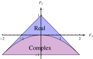
Figure 1: The range of the memory functions for which the condition $C(n)\rightarrow\ 0$ as $n\rightarrow\infty$ is satisfied (when the zeros of the characteristic polynomial are inside the circle $|\lambda|<1$ on the complex plane).

In the case of the 2nd order chain, system of equations (23) reduces to a single equation

$$C(1)=F_{1}C(0)+F_{2}C(0),$$ (35)

and, therefore, there is just one constant $\Gamma_{1}$ (see (26)):

$$\Gamma_{1}(F_{1},F_{2})=F_{1}(1-F_{2})^{-1}.$$ (36)

Solution (30) for the 2nd order chain is

$$C(n)=\gamma_{1}{\lambda_{1}}^{n}+\gamma_{2}{\lambda_{2}}^{n},\hskip 28.45274pt\lambda_{1,2}=\frac{F_{1}\pm\sqrt{F_{1}^{2}+4F_{2}}}{2},$$ (37)

where $\gamma_{1,2}$ are

$$\gamma_{1}=C(0)\frac{\lambda_{2}-\Gamma_{1}}{\lambda_{2}-\lambda_{1}},\hskip 28.45274pt\gamma_{2}=C(0)\frac{\Gamma_{1}-\lambda_{1}}{\lambda_{2}-\lambda_{1}}.$$ (38)

Correlation functions for different values of memory functions $F_{1}$ and $F_{2}$ are presented in Fig. 2.

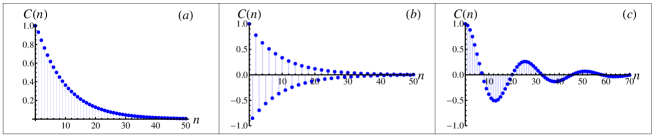
Figure 2: The correlation function $C(n)$ of the 2nd order sequence with different memory functions: a) $F_{1}=1,1$ and $F_{2}=-0,18$; b) $F_{1}=-0,7$ and $F_{2}=0,18$; c) $F_{1}=1,84$ and $F_{2}=-0,9$.

In the case of the 3rd order chain, for the roots of the cubic characteristic polynomial $p_{3}=\lambda^{3}-F_{1}\lambda^{2}-F_{2}\lambda-F_{3}$ to lie inside the unit circle on the complex plane, it is necessary and sufficient that the following conditions be satisfied [50]:

$$|F_{1}+F_{3}|<1-F_{2},\hskip 28.45274pt|F_{1}-3F_{3}|<3+F_{2},\hskip 14.22636pt{F_{3}}^{2}-F_{2}-F_{1}F_{3}<1.$$ (39)

The corresponding range of allowed values of the memory function is shown in Fig. 3.

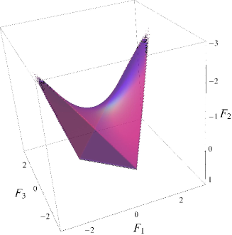
Figure 3: The range of the memory functions for which the condition $C_{n}\rightarrow\ 0$ as $n\rightarrow\infty$ is satisfied (when the zeros of the characteristic polynomial $p_{3}$ are inside the circle $|\lambda|<1$ on the complex plane).

For the 3rd order chain the system (23), determining the boundary conditions, has a form

$$\left(\begin{array}[]{cc}-F_{1}-F_{3}&1\\ 1-F_{2}&-F_{3}\end{array}\right)\left(\begin{array}[]{c}C(1)\\ C(2)\end{array}\right)=C(0)\left(\begin{array}[]{c}F_{2}\\ F_{1}\end{array}\right)$$ (40)

and constants $\Gamma_{1,2}$, (27), are

$$\Gamma_{1}(F_{1},F_{2},F_{3})=\frac{F_{1}+F_{2}F_{3}}{\Delta},\hskip 28.45274pt\Gamma_{2}(F_{1},F_{2},F_{3})=\frac{F_{1}^{2}+F_{1}F_{3}-F_{2}^{2}}{\Delta},$$ (41)

where

$$\Delta=1-F_{2}-(F_{1}+F_{3})F_{3}.$$ (42)

Solution (30) for the 3rd order chain is

$$C(n)=\gamma_{1}{\lambda_{1}}^{n}+\gamma_{2}{\lambda_{2}}^{n}+\gamma_{3}{\lambda_{3}}^{n},$$ (43)

where constants $\gamma_{1,2,3}$ are

$$\begin{array}[]{l}\gamma_{1}=C(0)\displaystyle\frac{\Gamma_{2}+\lambda_{2}\lambda_{3}-\Gamma_{1}(\lambda_{2}+\lambda_{3})}{(\lambda_{1}-\lambda_{2})(\lambda_{1}-\lambda_{3})},\\[17.07164pt] \gamma_{2}=C(0)\displaystyle\frac{\Gamma_{2}+\lambda_{1}\lambda_{3}-\Gamma_{1}(\lambda_{1}+\lambda_{3})}{(\lambda_{1}-\lambda_{2})(\lambda_{2}-\lambda_{3})},\\[17.07164pt] \gamma_{3}=C(0)\displaystyle\frac{\Gamma_{2}+\lambda_{1}\lambda_{2}-\Gamma_{1}(\lambda_{1}+\lambda_{2})}{(\lambda_{1}-\lambda_{3})(\lambda_{2}-\lambda_{3})},\end{array}$$ (44)

and $\lambda_{1,2,3}$ are roots of the characteristic equation of the 3rd degree. They can be either three real roots, or one real and two complex conjugates. The solutions of the cubic equation are quite lengthy and known and we will not write down them here. The dependence of the correlation functions on the distance between the elements of the chain is similar to those shown in Fig. 2.

7.2 Examples of correlations in the $N$th order chains

Below, to illustrate possible correlation scenarios in the additive Markov chains, we present plots of correlation functions for the additive linear Markov chains of order $N=20$ for different types of memory functions. In each of the Figs. 4–7, the memory function is shown at the top left, the roots of the polynomial equations (29), corresponding to the respective memory functions, are at the top right and the dependence of the correlation function (30) on the distance between the elements of the chain is at the bottom.

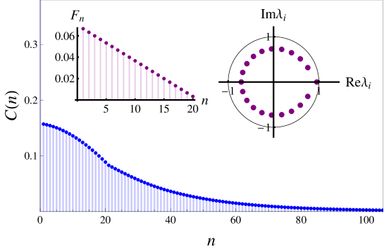
Figure 4: Linear memory function $F_{n}$ (top left), characteristic equation roots $\lambda$ on the complex plane (top right) and correlation function $C(n)$ (bottom).

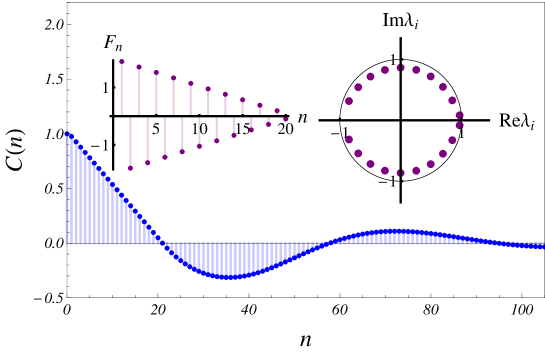
Figure 5: Alternating sign linear memory function $F_{n}$ (top left), characteristic equation roots $\lambda$ on the complex plane (top right) and correlation function $C(n)$ (bottom).

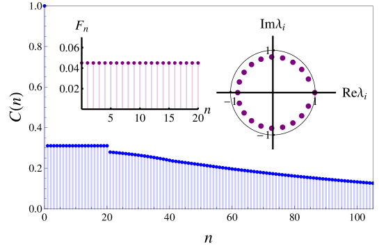
Figure 6: Step-wise memory functions $F_{n}$ (top left), characteristic equation roots $\lambda$ on the complex plane (top right) and correlation function $C(n)$ (bottom).

Figure 7: Alternating sign step-wise memory functions $F_{n}$ (top left), characteristic equation roots $\lambda$ on the complex plane (top right) and correlation function $C(n)$ (bottom).

8 Numerical generation of the chain with a given correlation function

The main purpose of the developed theory is to elaborate a reliable tool for the generation of numerical random sequences with prescribed correlation characteristics. The previous consideration concerned mostly the so-called direct problem, that is, the problem of finding the correlation function of the generated sequence with a given CPDF. In this section we address the inverse problem, namely, the problem of retrieving the CPDF of the sequence provided the correlation functions are given. For the linear high-order Markov chains (2), the inverse problem can be formulated as follows:

Proposition 5. To find the weight functions $f_{\mu}(x)$ we should solve the system of equations (22) and (19).

Up to here our theory was based on the ensemble statistical averaging. Now we would like to change our method of reasoning and show a generation of one chain of random variables possessing the same statistical characteristic as the an ensemble of chains. It is evident that the generated sequence have to be ergodic.

According to the ergodic theorem (see, e.g., Ref. [30, 32]), the finiteness of $N$ together with the strict inequalities,

$$0<\mathbb{P}\left(X_{n}=x_{n}|\left\{X_{i}=x_{i}\right\}_{n-N}^{n-1}\right)<1,\,\,n\in\mathbb{Z},$$ (45)

provides ergodicity of the random sequence. The stationarity and ergodicity are the sufficient conditions for formulation of the two well known important statements of information theory: asymptotic equipartition property (the Shannon-McMillan-Breiman theorem), [27] and the Kac’s lemma [51, 52]. Analogously, we should impose these conditions for generating the random stationary ergodic sequence.

Let us demonstrate this with an example of numerical generation of the Markov sequence with memory length $N=2$.

We choose the probability distribution function of the uncorrelated chain in a symmetric “triangular” form, see Fig. 4 (left):

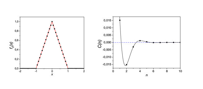
Figure 8: Numerical generation of the 2nd order chain: the one-point probability distribution function $f_{0}(x)$ (on the left); comparison of the numerical (points) and analytical (line) correlation functions (on the right).

$$f_{0}(x)=\left\{\begin{array}[]{cr}1-|x|,&|x|<1,\\[8.53581pt] 0,&|x|\geqslant 1.\end{array}\right.$$ (46)

This probability distribution function of uncorrelated chain corresponds to the zero mean value of random variable $\langle X\rangle=0$ and coincides with the one-point probability function $P(X=x)$. The standard deviation is $C(0)=\sigma^{2}=1/6$. The values of the memory function are chosen as $F_{1}=0,1$ and $F_{2}=-0,1$.

To generate, it remains to specify weight functions $f_{1}$ and $f_{2}$, which are part of the CPDF (2). As can be seen from Eq.  (19), there is a great freedom in the choice of the functions $f_{1}$ and $f_{2}$ which ensure the given values of $F_{1}$ and $F_{2}$. However, their form should be such that (2) yields a positive result for any value $x\in(-1;1)$ and any combination of two preceding values $x_{1,2}\in(-1;1)$ . This implies, in particular, that for the values of $x$ which give close to zero values of $f_{0}(x)$ (in our case, these values of $x$ are close to $\pm 1$) the absolute value of $f_{1,2}(x)$ should also be close to zero. The simplest way to ensure this condition is to choose $f_{1,2}(x)$ proportional to $f_{0}(x)$, but odd, to ensure normalization conditions (6):

$$f_{1,2}(x)=a_{1,2}\left\{\begin{array}[]{cr}f_{0}(x),&x\geqslant 0,\\[5.69054pt] -f_{0}(x),&x<0,\end{array}\right.$$ (47)

and the coefficient $a_{1,2}$ is then determined from the condition (19) to ensure the required $F_{1}$ and $F_{2}$. In the case under consideration the triangular one-point distribution function leads to $a_{1,2}=3F_{1,2}$.

Substituting now the required values of $F_{1}$ and $F_{2}$, we obtain the CPDF (2) and with its use generate the numerical sequence. Having it constructed, we numerically calculate the correlation functions. In Fig. 8 (right) the points show obtained values of $C(n)$. The solid line corresponds to the analytical results for the correlation functions, obtained in previous subsection. It is seen that the results of numerical modeling of the correlated sequence perfectly coincide with those obtained analytically.

9 Conclusion

We have shown that the additive linear CPDF given by Eq. (2) can generate a stationary ergodic random sequence with the one-point distribution function, Eq. (12), and the pair correlation functions satisfying Eq. (16) with the boundary conditions Eq. (22). The general solution of Eq. (16) is given by the linear combination of the corresponding particular solutions Eq. (30) with the coefficients explicitly determined by Eq. (33). The obtained analytical solutions for the equations connecting the memory and correlation functions are compared with the results of numerical simulation. Examples of possible correlation scenarios in the high-order additive linear chains are given.

References

- [1] U. Balucani, M. H. Lee, V. Tognetti, Phys. Rep. 373, 409 (2003).
- [2] I. M. Sokolov, Phys. Rev. Lett. 90, 080601 (2003).
- [3] A. Bunde, S. Havlin, E. Koscienly-Bunde, H.-J. Schellenhuber, Physica A 302, 255 (2001).
- [4] H. N. Yang, Y.-P. Zhao, A. Chan, T.-M. Lu, and G. C. Wang, Phys. Rev. E 56, 4224 (1997).
- [5] S. N. Majumdar, A. J. Bray, S. J. Cornell, and C. Sire, Phys. Rev. Lett. 77, 3704 (1996).
- [6] S. Halvin, R. Selinger, M. Schwartz, H. E. Stanley, and A. Bunde, Phys. Rev. Lett. 61, 1438 (1988).
- [7] R. F. Voss, Phys. Rev. Lett. 68, 3805 (1992).
- [8] H. E. Stanley et. al., Physica A 224, 302 (1996).
- [9] S. V. Buldyrev, A. L. Goldberger, S. Havlin, R. N. Mantegna, M. E. Matsa, C.-K. Peng, M. Simons, H. E. Stanley, Phys. Rev. E 51, 5084 (1995).
- [10] A. Provata and Y. Almirantis, Physica A 247, 482 (1997).
- [11] R. M. Yulmetyev, N. Emelyanova, P. Hänggi, and F. Gafarov, A. Prohorov, Phycica A 316, 671 (2002).
- [12] B. Hao, J. Qi, Mod. Phys. Lett. 17, 1 (2003).
- [13] R. N. Mantegna, H. E. Stanley, Nature (London) 376, 46 (1995).
- [14] Y. C. Zhang, Europhys. News, 29, 51 (1998).
- [15] A. Schenkel, J. Zhang, and Y. C. Zhang, Fractals, 1, 47 (1993).
- [16] I. Kanter and D. A. Kessler, Phys. Rev. Lett. 74, 4559 (1995).
- [17] P. Kokol, V. Podgorelec, Complexity International, 7, 1 (2000).
- [18] W. Ebeling, A. Neiman, T. Poschel, arXiv:cond-mat/0204076.
- [19] O. V. Usatenko, V. A. Yampol’skii, K. E. Kechedzhy and S. S. Mel’nyk, Phys. Rev. E 68, 061107 (2003).
- [20] O. V. Usatenko and V. A. Yampol’skii, Phys. Rev. Lett. 90, 110601 (2003).
- [21] C. D. Manning, P. Raghavan, and H. Schutze, Introduction to Information Retrieval, (Cambridge University Press, Cambridge, 2008).
- [22] P. Ehrenfest and T. Ehrenfest, Encyklopädie der Mathematischen Wissenschaften (Springer, Berlin, 1911), p. 742, Bd. II.
- [23] D. Lind and B. Marcus, An Introduction to Symbolic Dynamics and Coding (Cambridge University Press, Cambridge, 1995).
- [24] D. Salomon, A Concise Introduction to Data Compression, (Springer, Berlin, 2008).
- [25] F. M. Izrailev, A. A. Krokhin and N. M. Makarov, Physics Reports 512, 125 (2012).
- [26] B. B. Mandelbrot, J. R. Wallis, Water Resour. Res. 7, 543 (1971).
- [27] T. M. Cover, J. A. Thomas, Elements of Information Theory, second edition (New York, Wiley, 2006).
- [28] A. Raftery, J. R. Stat. Soc. B 47, 528 (1985).
- [29] M. Seifert, A. Gohr, M. Strickert, I. Grosse, PLoS Computat. Biol, 8, e1002286 (2012).
- [30] P. C. Shields, The ergodic theory of discrete sample paths (Graduate studies in mathematics, 13, 1996).
- [31] S. S. Melnik, O. V. Usatenko, V. A. Yampol’skii, and V. A. Golick, Phys. Rev. E 72, 026140 (2005).
- [32] A. N. Shiryaev, Probability (Springer, New York, 1996).
- [33] R. F. Voss in: Fundamental Algorithms in Computer Graphics (Berlin: Springer, 1985 ) 805.
- [34] M. F. Shlesinger, G. M. Zaslavsky and J. Klafter, Nature, 363, 31 (1993).
- [35] W. Li, Europhys. Let. 10, 395 (1989).
- [36] H. A. Makse, S. Havlin, M. Schwartz and H.E. Stanley, Phys. Rev. E 53, 5445 (1996).
- [37] O. V. Usatenko, S. S. Apostolov, Z. A. Mayzelis, and S. S. Melnik, Random Finite-Valued Dynamical Systems: Additive Markov Chain Approach (Cambridge Scientific Publisher, Cambridge, 2010).
- [38] D.F. Anderson and T.G. Kurtz, in H. Koeppl, G. Setti, M di Bernardo, D Densmore. (eds), Design and Analysis of Biomolecular Circuits, Chapter 1, (New York, NY: Springer, 2011).
- [39] A. A. Atayero and O. I. Sheluhin, Integrated Models for Information Communication Systems and Networks: Design and Development, (Hershey, PA: IGI Publishing, 2013).
- [40] P. Carpena, P. Bernaola-Galv́an, P.Ch. Ivanov and H.E. Stanley, Nature, 418, 955 (2002).
- [41] P. Carpena, P. Bernaola-Galv́an, P.Ch. Ivanov and H.E. Stanley, Nature, 421, 764 (2002).
- [42] S. Hod and U. Keshet, Phys. Rev. E 70, 015104(R) (2004).
- [43] S. L. Narasimhan, J. A. Nathan and K.P.N. Murthy, Europhys. Lett. 69, 22 (2005).
- [44] S. L. Narasimhan, J. A. Nathan, P. S. R. Krishna and K. P. N. Murthy, 367, 252 (2006).
- [45] F. M. Izrailev, A. A. Krokhin, N. M. Makarov, and O.V. Usatenko, Phys. Rev. E 76, 027701-1 (2007).
- [46] A. A. Apostolov, F. M. Izrailev, N. M. Makarov, Z. A. Mayzelis, S. S. Melnyk and O. V. Usatenko, J. Phys. A: Math. Theor. 41 175101 (2008).
- [47] Saber Elaydi, An Introduction to Difference Equations, 3rd Edition, Springer-Verlag New York, 2005.
- [48] P. Stoica and R.L. Moses, Signal Processing, 26, 95 (1992).
- [49] Y. Bistritz, Circuits Systems Signal Process, 15, 111 (1996).
- [50] E. A. Grove, G. Ladas, Advances in Discrete Mathematic and Applications V. 4, Periodicities in Nonlinear Difference Equations, Chapman and Hall/CRC, 2005.
- [51] M. Kac, Bull. Am. Math. Soc. 53, 1002 (1947).
- [52] F. Cecconi, M. Cencini, M. Falcioni, and A. Vulpiani, Am. J. Phys. 80, 1001 (2012).