Performance Analysis of Intelligent Reflective Surfaces for Wireless Communication

Abstract

A statistical characterization of the fundamental performance bounds of an intelligent reflective surface (IRS) intended for aiding wireless communications is presented. To this end, the outage probability, average symbol error probability and achievable rate bounds are derived in closed-form. By virtue of an asymptotic analysis in high signal-to-noise ratio (SNR) regime, the achievable diversity order is derived. Thereby, we show that a diversity gain in the order of the number of passive reflective elements embedded within the IRS can be achieved with only controllable phase adjustments. Thus, IRS has a great potential of boosting the wireless performance by intelligently controlling the propagation channels without employing additional active radio frequency chains.

I Introduction

Over the past five generations of wireless standards, performance of the transmitter and receiver has been optimized to mitigate various transmission impairments of propagation channels, which are generally assumed to be uncontrollable in the wireless system designer’s perspective. However, owing to the recent research advancements of meta-materials and meta-surfaces, a novel concept of coating physical objects such as building walls and windows with intelligent reflective surfaces (IRSs) with reconfigurable reflective properties has been envisioned [1, 2, 3, 4]. The ultimate goal of IRS is to enable a smart wireless propagation environment by controlling the reflective properties of the underlying channels [4].

An IRS comprises of a very large number of passive reflective elements, which are capable of reconfiguring properties of electromagnetic (EM) waves impinging upon them. On one hand, reflected EM waves can be added constructively at a desired receiver by intelligently controlling phase-shifts at each reflective element to boost the signal-to-noise ratio (SNR) and coverage. On the other hand, a reflected signal can be made to add destructively and thereby to mitigate co-channel interference towards an undesired direction. Moreover, IRS facilitates full-duplex reflections, and hence, large blockages between a pair of transmitter-receiver can be circumvented through smart reflections without trading-off additional time, frequency or power resources. Since an IRS does not generate new EM waves, costly transmit radio-frequency (RF) chains/amplifiers in relays can be eliminated and thereby improving the energy efficiency. Thus, the concept of IRS presents a paradigm shift in wireless communication research.

Prior related research: Due to recent breakthroughs in physics and related fields [5, 6, 7], the designs of software-controllable IRS have been shown to be feasible, and core technical aspects are currently being developed [8, 1]. The prototypes of meta-surfaces and meta-tiles with artificial thin film of EM materials, which can be used to coat objects within a smart wireless environment, have already been developed [5, 6]. In [9], precoder optimization techniques for a multi-antenna transmitter in the presence of an IRS are investigated to maximize the received SNR. In [10], basic ray tracing techniques are adopted to model multipath propagation through an IRS, and thereby, it discusses techniques for controlling the reflections via controllable phase-shifts at passive elements embedded within an IRS. Moreover, in [11], transmit power scaling laws pertaining to IRS are derived to alleviate misconceptions about the performance comparisons between the IRS and massive multiple-input multiple-output (MIMO) systems. In [12], an optimal phase shift design is proposed for IRS based on maximizing an upper bound of the average spectral efficiency. In [13], techniques for boosting the physical layer security through smart propagation enabled by an IRS are investigated.

Motivation and our contribution: The key idea of an IRS is to enable a programmable control over the wireless propagation channels. This necessitates innovations of radically novel techniques for modeling, designing and analyzing wireless systems as the resulting smart propagation channels can now be able to interact with EM waves impinging upon them in a software-controlled manner. Although several important attempts have recently been made [9, 10, 11, 12, 13], the fundamental research on IRS in wireless communication’s perspective is still at an embryonic stage. To this end, our work presents a performance analysis framework for deriving the fundamental bounds pertaining to an IRS intended for aiding the end-to-end communication between a single-antenna source ($S$) and a destination ($D$). Thus, tight bounds/approximations for the outage probability, average symbol error rate (SER), and average achievable rate are derived in closed-form. The accuracy of our analysis is validated through a rigorous set of Monte-Carlo simulations. We obtain useful design insights about the achievable diversity order via an asymptotic analysis in the high SNR regime. We reveal that the achievable diversity order is equal to the number of passive reflective elements ($M$), and it is achieved without using any active RF chains at the IRS. Thus, by virtue of smart passive reflections, an $M$-fold diversity gain can be achieved with respect to a single-input single-output (SISO) channel. Through our analysis, we verify that an IRS has a true potential of boosting the reliability of end-to-end wireless communication with only passive controllable phase-shifts.

Notation: $\mathbf{x}^{T}$ denotes the transpose of $\mathbf{x}$. $\mathbb{E}\!\left[{X}\right]$ and $\mathbb{V}\mathrm{ar}\!\left[{X}\right]$ represent the expectation and variance of a random variable (RV) $X$, respectively. $X\sim\mathcal{CN}\left(\mu_{X},\sigma_{X}^{2}\right)$ denotes that $X$ is complex Gaussian distributed with $\mu_{X}$ mean and $\sigma_{X}^{2}$ variance.

II System, channel and signal models

Figure 1: An IRS-assisted wireless communication set-up.

II-A System model

We consider an end-to-end wireless communication set-up in which a single-antenna source ($S$) communicates with a single-antenna destination ($D$) through an IRS having $M$-passive reflective elements (see Fig. 1). Phase-shifts of waves impinging upon the IRS are assumed to be controlled perfectly to implement coherent/constructive signal combining at $D$, while the corresponding amplitudes are attenuated by a factor defined as per reflective coefficient. The direct channel between $S$ and $D$ is assumed to be unavailable due to severe blockage effects. The channel between $S$ and the $m$th reflective element is denoted by $h_{m}$, while the channel between the $m$th reflective element and $D$ is given by $g_{m}$. The channel envelopes are assumed to be independent Rayleigh distributed, and hence, $h_{m}$ and $g_{m}$ are modeled as

$$h_{m}=\sqrt{\zeta_{h_{m}}}\tilde{h}_{m}\qquad\text{and}\qquad g_{m}=\sqrt{\zeta_{g_{m}}}\tilde{g}_{m},$$ (1)

where $\tilde{h}_{m}$ and $\tilde{g}_{m}$ follow complex Gaussian distribution with zero mean and unit variance; $\tilde{h}_{m}\sim\mathcal{CN}(0,1)$ and $\tilde{g}_{m}\sim\mathcal{CN}(0,1)$. In (1), $\zeta_{h_{m}}$ and $\zeta_{g_{m}}$ capture the path-losses of the corresponding channels.

II-B Signal model

The signal transmitted by $S$ is reflected by the IRS towards $D$. The received signal at $D$ through $M$ reflective elements can be written as

$$y=\sqrt{P}\displaystyle\sum_{m=1}^{M}g_{m}\eta_{m}\mathrm{e}^{j\theta_{m}}h_{m}x+n,$$ (2)

where $x$ is the transmitted signal by $S$ satisfying $\mathbb{E}\!\left[{|x|^{2}}\right]=1$, while $P$ is the transmit power at $S$. Moreover, $n$ is an additive white Gaussian noise (AWGN) at D with zero mean and variance $\sigma_{N}^{2}$ such that $n\sim\mathcal{CN}(0,\sigma_{N}^{2})$. In (2), $\eta_{m}$ and $\theta_{m}$ represent the reflection coefficient and the phase-shift introduced by the $m$th reflective component of the IRS, respectively. Next, (2) can be alternatively written as [9]

$$y=\sqrt{P}\mathbf{g}^{T}\mathbf{\Theta}\mathbf{h}x+n,$$ (3)

where $\mathbf{h}$ = [$h_{1}$, $\cdots$, $h_{m}$, $\cdots$, $h_{M}$]^T and $\mathbf{g}$ = [$g_{1}$, $\cdots$, $g_{m}$, $\cdots$, $g_{M}$]^T capture the corresponding channel vectors, while $\mathbf{\Theta}=\text{diag}([\eta_{1}\mathrm{e}^{j\theta_{1}},\cdots,\eta_{m}\mathrm{e}^{j\theta_{m}},\cdots,\eta_{M}\mathrm{e}^{j\theta_{M}}])$ is a diagonal matrix, which captures the reflection properties of $M$ reflective elements of the IRS.

By using (3), the SNR is derived as

$${\Gamma}={\bar{\gamma}|\mathbf{g}^{T}\mathbf{\Theta}\mathbf{h}|^{2}},$$ (4)

where $\bar{\gamma}=P/\sigma_{N}^{2}$ is the average transmit SNR. The channels $h_{m}$ and $g_{m}$ in (1) can be rewritten as

$$h_{m}=\nu_{m}\text{exp}\!\left({j\phi_{m}}\right)\qquad\text{and}\qquad g_{m}=\rho_{m}\text{exp}\!\left({j\omega_{m}}\right),$$ (5)

where $\nu_{m}=|h_{m}|$ and $\rho_{m}=|g_{m}|$ are the channel amplitudes with Rayleigh distribution, while $\phi_{m}$ and $\omega_{m}$ are the corresponding channel phases, which are uniformly distributed between $\left(\right.\!\!-\pi,\pi\left.\right]$. By substituting (5) into (4), the SNR in (4) can be expanded as

$${\Gamma}={\bar{\gamma}\left|\displaystyle\sum_{m=1}^{M}\rho_{m}\nu_{m}\eta_{m}\text{exp}\!\left({j[\phi_{m}+\omega_{m}+\theta_{m}]}\right)\right|^{2}}.$$ (6)

The $M$ terms inside the summation of (6) must be constructively added to maximize the received SNR. This can be accomplished by intelligently controlling the reflective properties ($\theta_{m}$) of each element within the IRS. More specifically, $\Gamma$ in (6) can be maximized by co-phasing each term in its summation. Thus, the optimal choice of $\theta_{m}$ is given by $\underset{-\pi<\theta_{m}\leq\pi}{\text{arg}\!\max}\;\{\Gamma\}=\theta^{*}_{m}=-(\phi_{m}+\omega_{m})$ [9], and thereby, the optimal received SNR at $D$ can be written as

$$\Gamma^{*}={\bar{\gamma}\left|\displaystyle\sum_{m=1}^{M}\rho_{m}\nu_{m}\eta_{m}\right|^{2}}.$$ (7)

III Performance Analysis

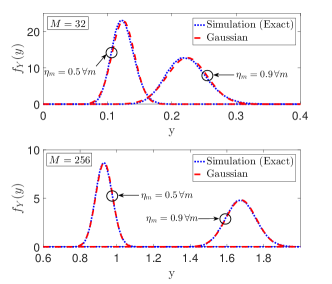
Figure 2: The exact PDF of $Y=\sum_{m=1}^{M}\rho_{m}\nu_{m}\eta_{m}$ via Monte-Carlo simulations and its analytical approximation via CLT.

III-A Statistical characterization of the optimal received SNR

We notice that $\rho_{m}$ and $\nu_{m}$ are independently Rayleigh distributed RVs for $m\in\{1,\cdots,M\}$. Thus, according to the central limit theorem (CLT), $Y=\sum_{m=1}^{M}\rho_{m}\nu_{m}\eta_{m}$ coverages to a Gaussian distribution for a sufficiently large number of passive elements in the IRS [14]. Thereby, the distribution of $\Gamma^{*}$ in (7) can be tightly approximated by a non-central chi-squared distribution with a single degree-of-freedom [14]; $\Gamma^{*}\approx\gamma\sim\mathcal{X}^{2}_{1}(\nu)$, where $\nu$ is the non-centrality parameter. The accuracy of this approximation is verified via the probability density function (PDF) curves in Fig. 2 for different $M$ and $\eta_{m}$. Consequently, the cumulative distribution function (CDF) of $\gamma$ can be written as (see Appendix A)

$$F_{\gamma}(z)=1-\psi\mathcal{Q}\left(\left({\sqrt{z/\bar{\gamma}}-\mu_{Y}}\right)\Big{/}{\sigma_{Y}}\right),$$ (8)

where $z\geq 0$, and $\mathcal{Q}\left(\cdot\right)$ denotes the Gaussian $\mathcal{Q}$ function, which is defined as $\mathcal{Q}\left(x\right)=\int_{x}^{\infty}\mathrm{e}^{-t^{2}/2}\big{/}{\sqrt{2\pi}}dt$ [15]. In (8), $\mu_{Y}$, $\sigma_{Y}$, and $\psi$ are given by

$$\!\!\!\!\!\!\!\!\!\!\mu_{Y} = \sum_{m=1}^{M}\pi\lambda_{m}/2\quad\text{and}\quad\sigma^{2}_{Y}=\sum_{m=1}^{M}\lambda^{2}_{m}\left[16-{\pi}^{2}\right]/4,\;$$ (9a)

$$\!\!\!\!\!\!\!\!\!\!\!\!\psi = 1/\left[\mathcal{Q}\left(-\sqrt{\kappa}\right)\right],$$ (9b)

where $\lambda^{2}_{m}=\zeta_{h_{m}}\zeta_{g_{m}}\eta_{m}^{2}/4$, $\kappa=\mu^{2}_{Y}/\sigma^{2}_{Y}$ and $\Gamma\!\left({t}\right)=\int_{0}^{\infty}x^{t-1}\mathrm{e}^{-x}dx$ is the Gamma function [16, Eqn. (8.310.1)].

III-B Outage Probability

The SNR outage is defined as the probability that the instantaneous SNR $(\gamma)$ falls bellow a threshold SNR $(\gamma_{th})$. By using (8), a tight approximation for the outage probability in moderately large $M$ regime can be obtained as

$$P_{out}=\Pr(\Gamma^{*}\leq\gamma_{th})\approx F_{\gamma}\!\left({\gamma_{th}}\right),$$ (10)

where $F_{\gamma}\!\left({\cdot}\right)$ is defined in (8).

Remark 1: The PDF of $\Gamma^{*}$ in (7) for $M=1$ is given by $f_{\Gamma^{*}}(z)=(2\bar{\gamma}\lambda^{2}_{1})^{-1}K_{0}(\sqrt{z/(\bar{\gamma}\lambda^{2}_{1}}))$ [17], and the exact outage probability can be derived by using [16, Eqn. (5.56.2)] as

$$P_{out}=F_{\Gamma^{*}}\!\left({\gamma_{th}}\right)=1-\sqrt{{\gamma_{th}}/{\bar{\gamma}\lambda^{2}_{1}}}K_{1}(\sqrt{{\gamma_{th}}/{\bar{\gamma}\lambda^{2}_{1}}}),$$ (11)

where $K_{v}\left(\cdot\right)$ is the $v$th order modified Bessel function of the second kind [16, Eqn. 8.407.1].

III-C Average achievable rate

The average achievable rate can be defined as

$$\mathcal{R}=\mathbb{E}\!\left[{\mathrm{log}_{2}\left(1+\Gamma^{*}\right)}\right]\approx\mathbb{E}\!\left[{\mathrm{log}_{2}\left(1+\gamma\right)}\right].$$ (12)

The exact derivation of the expectation in (12) appears mathematically intractable. Thus, we resort to upper and lower bounds by invoking Jensen’s inequality as $\mathcal{R}_{lb}\apprle\mathcal{R}\apprle\mathcal{R}_{ub}$ [18], where $\mathcal{R}_{lb}$ and $\mathcal{R}_{ub}$ are defined as

$$\mathcal{R}_{lb} = {\mathrm{log}_{2}\left(1+\left[\mathbb{E}\!\left[{{1}\big{/}{\gamma}}\right]\right]^{-1}\right)},$$ (13)

$$\mathcal{R}_{ub} = \mathrm{log}_{2}\left(1+\mathbb{E}\!\left[{\gamma}\right]\right).$$ (14)

The upper bound in (14) can be derived as (see Appendix B)

$$\mathcal{R}_{ub} = \mathrm{log}_{2}\left(1+\left(\bar{\gamma}\sum_{m=1}^{M}\lambda^{2}_{m}\right)\left[\frac{(16-\pi^{2})(1+\kappa)}{4}\right]\right).$$ (15)

Next, a tight approximation for the lower bound in (13) can be derived as (see Appendix B)

$$\!\!\!\!\!\!\!\mathcal{R}_{lb}\approx\mathrm{log}_{2}\left(\!1\!+\left(\bar{\gamma}\sum_{m=1}^{M}\lambda^{2}_{m}\right)\left[\frac{(16-\pi^{2})(\kappa+1)^{3}}{4(\kappa^{2}+6\kappa+3)}\right]\right).$$ (16)

III-D Average symbol error rate (SER)

The average SER is defined as the expectation of conditional error probability $(P_{e|\Gamma^{*}})$ over the distribution of $\Gamma^{*}$ [15]. For wide range of modulation schemes, $P_{e|\gamma}$ is given by $P_{e|\Gamma^{*}}=\alpha\mathcal{Q}\left(\sqrt{\beta\Gamma^{*}}\right)$, where $\alpha$ and $\beta$ are modulation dependent fixed parameters [15]. In this context, the average SER can be derived as $\bar{P}_{e}=\mathbb{E}\!\left[{\alpha\mathcal{Q}\left(\sqrt{\beta\Gamma^{*}}\right)}\right]$. By using (8) and by evaluating the expectation, a tight approximation for $\bar{P}_{e}$ can be derived as (see Appendix C)

$$\bar{P}_{e} \approx \mathbb{E}\!\left[{\alpha\mathcal{Q}\left(\sqrt{\beta\gamma}\right)}\right]$$ (17)

$$= \frac{\alpha{\psi}\mathrm{exp}(-\mu_{Y}^{2}/2\sigma_{Y}^{2})}{\sqrt{2}{\pi}\sigma_{Y}}\int_{0}^{\pi/2}\frac{\mathrm{exp}\left(\mu_{Y}^{2}\big{/}\left(\frac{2\beta\bar{\gamma}\sigma_{Y}^{4}}{\sin^{2}\theta}+2\sigma_{Y}^{2}\right)\right)}{\sqrt{\frac{\beta\bar{\gamma}}{2\sin^{2}\theta}+\frac{1}{2\sigma_{Y}^{2}}}}$$

$$\quad\quad\quad\times\mathcal{Q}\left({\mu_{Y}}\big{/}{\sqrt{\frac{\beta\bar{\gamma}\sigma_{Y}^{4}}{\sin^{2}\theta}+{\sigma_{Y}^{2}}}}\right)d\theta.$$

We upper bound (17) by setting $\theta\!=\!\pi/2$ as (see Appendix C)

$$\bar{P}^{ub}_{e} = \frac{\alpha{\psi}\mathrm{exp}(-\mu_{Y}^{2}/2\sigma_{Y}^{2})}{2\sigma_{Y}}\frac{\mathrm{exp}\left(\mu_{Y}^{2}\big{/}\left({2\beta\bar{\gamma}\sigma_{Y}^{4}}+2\sigma_{Y}^{2}\right)\right)}{\sqrt{{\beta\bar{\gamma}}+{1}/{\sigma_{Y}^{2}}}}$$ (18)

$$\quad\quad\quad\times\mathcal{Q}\left({\mu_{Y}}\big{/}{\sqrt{{\beta\bar{\gamma}\sigma_{Y}^{4}}+{\sigma_{Y}^{2}}}}\right).$$

Remark 2: The exact average SER for $M=1$ can be derived by evaluating $\bar{P}_{e}=\mathbb{E}\!\left[{\alpha\mathcal{Q}\left(\sqrt{\beta\Gamma^{*}}\right)}\right]$ using $F_{\Gamma^{*}}\!\left({z}\right)$ and invoking [16, Eqn. (6.614.5)] as follows:

$$\bar{P}_{e}=\frac{\alpha}{2}-\frac{\alpha\,\delta}{2}\mathrm{exp}{\left(\delta\right)}\left(K_{1}(\delta)-K_{0}(\delta)\right),$$ (19)

where $\delta=(4\beta\bar{\gamma}\lambda^{2}_{1})^{-1}$.

III-E Achievable diversity order

The diversity order is defined as the negative slope of the outage probability or average SER versus the average SNR curve in a log-log scale as [19]

$$G_{d}=\lim_{\bar{\gamma}\rightarrow\infty}-\frac{\mathrm{log}\left(P_{out}\right)}{\mathrm{log}\left(\gamma\right)}=\lim_{\bar{\gamma}\rightarrow\infty}-\frac{\mathrm{log}\left(\bar{P}_{e}\right)}{\mathrm{log}\left(\gamma\right)},$$ (20)

from which useful information about how the outage probability or average SER decays in high SNR regime can be obtained. Since the outage probability and the average SER have identical diversity orders [19], we first proceed our diversity order derivation by using $P_{out}$.

In general, the outage probability can be asymptotically approximated in the high SNR regime as $P_{out}\approx(O_{c}\bar{\gamma})^{-G_{d}}$, where $G_{d}$ is the diversity order and $O_{c}$ is a measure of the coding gain [19]. A single-polynomial approximation of $P_{out}$ in (10) can be derived as (see Appendix D)

$$P^{\infty}_{out}=\Omega_{op}\left(\frac{\gamma_{th}}{\bar{\gamma}}\right)^{G_{d}}+\mathcal{O}\left(\bar{\gamma}^{-(G_{d}+1)}\right),$$ (21)

where the diversity order $G_{d}$ is given by

$$G_{d}=M,$$ (22)

where $M$ is the number of passive reflective elements in the IRS. In (21), $\Omega_{op}=\xi\prod_{m=1}^{M}(\lambda^{2}_{m}(2M)!)^{-1}$, where the constant $\xi$ depends on the coding/array gain.

Similarly, an asymptotic approximation for the average SER in high SNR regime can be derived as (see Appendix D)

$$\bar{P}^{\infty}_{e}=\left(G_{c}\bar{\gamma}\right)^{-M}+\mathcal{O}\left(\bar{\gamma}^{-(G_{d}+1)}\right),$$ (23)

where the coding gain is given by $G_{c}=(\alpha\Omega_{op}2^{M-1}\Gamma(M+1/2)/(\sqrt{\pi}\beta^{M}))^{-1/M}$.

Remark 3: The achievable diversity gain is in the order of the number of passive reflective embedded in the IRS even though both $S$ and $D$ are each equipped with a single-antenna. It is worth noting that each passive reflective element reconfigures phases of incident waves such that they add coherently at $D$. The direct SISO transmission between $S$ and $D$ permits only a unit diversity order. In conventional wireless systems, diversity gains can only be achieved by either transmit beamforming or via receive combining by employing multiple transmit/receive RF chains. However, the IRS is able to provide a significant diversity order by virtue of just passive reflectors with reconfigurable phases.

Figure 3: Geometric placement of nodes for numerical results.

Figure 4: An average SER comparison by letting $\alpha=1$ and $\beta=2$ in (17) for $M=32$. For all cases, $d_{SD}=100$ m. The distances for Case-1 to Case-4 are set to $d_{SI}=d_{DI}=51$ m, $d_{SI}=d_{DI}=80$ m, and $d_{SI}=d_{DI}=170$ m.

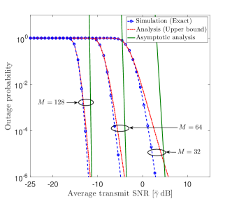
Figure 5: The outage probability with $\gamma_{th}\!=\!0$ dB, $d_{SI}\!=\!30$ m and $d_{DI}\!=\!20$ m.

Figure 6: The average rate with $d_{SI}=30$ m and $d_{DI}=20$ m.

IV Numerical results

In simulations, the path-loss is modeled as $\zeta\,[\text{dB}]=\zeta_{0}+10\upsilon\mathrm{log}\left(d\right)$, where $\zeta_{0}=42$ dB is a reference path-loss, $\upsilon=3.5$ is the path-loss exponent and $d$ is the distance. The geometric placement of nodes is depicted in Fig. 3. We set $\eta_{m}=\eta,\;\forall m$ for the sake of exposition.

Fig. 4 provides a comparison of the average SER for the IRS-assisted communication set-up (Case-1 to Case-3) with respect to a baseline direct transmission between $S$ and $D$ (Case-4). To highlight the performance gain of IRS over the direct transmission, in Case-1, the IRS is placed such that $d_{SI}+d_{DI}\approx d_{SD}$. Fig. 4 shows clearly that IRS-assisted communication outperforms its direct transmission counterpart. For example, at an average SER of $10^{-1}$, IRS-assisted system provides an approximately 28.56 dB (23.37 dB) reduction in the average transmit SNR for $\eta_{m}=0.9\;(\eta_{m}=0.5)\;\forall m$ in comparison to the direct transmission (see Case-1 and Case-4). When IRS is placed such that $d_{SD}<d_{SI}+d_{ID}<2d_{SD}$ (Case-2), the IRS-assisted communication can still provide a considerable average SER improvement compared to the direct transmission (see Case-2 and Case-4). This performance gain is obtained by means of the diversity gain rendered by smartly controlling the phase-shifts at each reflective element of the IRS to enable constructive addition of signals at $D$. However, when $d_{SI}+d_{ID}\gg d_{SD}$ (Case-3), the performance of IRS-assisted system is severely hindered mainly due to the substantial increase in distance-dependent path-loss effects (see Case-3 and Case-4). Fig. 4 also reveals that the average SER heavily depends on the reflection coefficient ($\eta_{m}$) of IRS elements. For instance, at an average SER of $10^{-4}$, an IRS with $\eta_{m}=0.9$ achieves a transmit SNR gain of 5.1 dB over that of an IRS with $\eta_{m}=0.5$.

In Fig. 5, the outage probability is plotted as a function of the average transmit SNR. Specifically, the proposed outage upper bound in (18) and its high SNR counterpart in (21) are plotted together with the exact Monte-Carlo simulations. Fig. 5 clearly depicts that the tightness of our proposed analytical outage improves in large $M$ regime. Counter-intuitively, it becomes looser in the high SNR regime. Nevertheless, our high SNR outage approximation tends to be asymptotically exact, and hence, it can be used to analytically quantify the diversity order and the corresponding outage performance in high SNR regime. Thus, the asymptotic outage curves in Fig. 5 verify that the IRS-assisted set-up achieves an $M$th order diversity gain. Fig. 5 reveals that the outage probability can be lowered significantly by increasing $M$. For instance, a quadruple and double increments in $M$ provide 13 dB and 7 dB reductions in the average transmit SNR to attain the same outage probability of $10^{-4}$.

In Fig. 6, the average achievable rate is plotted for different number of reflective elements at IRS as $M=[32,64,128,256]$. The exact achievable rate is plotted from (12) by using Monte-Carlo simulations. The analytical curves for the upper and lower bounds are plotted by using (15) and (16), respectively. Fig. 6 clearly illustrates that our upper bound is tight even for a moderately large number of IRS elements such as $M=32$. Moreover, the tightness of our lower bound improves with increasing $M$. Both upper and lower bounds approach the exact simulation when the number of IRS elements grows large (see $M=256$ case).

V Conclusion

The performance of IRS for wireless communication has been investigated by deriving the outage probability, average SER and achievable rate bounds and approximations. The accuracy of these metrics becomes tighter when the number of reflective elements in the IRS grows large. By deriving single-polynomial high SNR approximations of the CDF and PDF of the SNR, the achievable diversity order has been quantified. This high SNR analysis reveals that the achievable diversity order is equal to the number of passive reflective elements. A set of rigorous numerical results is provided to validate our performance analysis and to obtain useful insights about employing IRS for boosting the performance of next-generation wireless systems.

Appendix A Derivation of the CDF of $\gamma$ in (8)

We rewrite $\gamma\!=\!\bar{\gamma}Y^{2}$, where $Y\!=\!\sum_{m=1}^{M}X_{m}$ and $X_{m}\!=\!\rho_{m}\nu_{m}\eta_{m}$. Here, $\rho_{m}$ and $\nu_{m}$ in (7) are two independent Rayleigh distributed RVs with parameters $\zeta_{h_{m}}/2$ and $\zeta_{g_{m}}/2$, respectively. The $k$th moment of $X_{m}$ is given by [17]

$$\bar{x}_{k,m}=\mathbb{E}\!\left[{X^{k}_{m}}\right]=(\zeta_{h_{m}}\zeta_{g_{m}}\eta^{2}_{m})^{k/2}\left[\Gamma\!\left({k/2+1}\right)\right]^{2}.$$ (24)

By invoking CLT, the PDF of $Y$ can be approximated by a Gaussian distribution in moderately large $M$ regime; $Y\sim\mathcal{N}(\mu_{Y},\sigma_{Y}^{2})$, where $\mu_{Y}$ and $\sigma_{Y}^{2}$ are given by

$$\!\!\!\!\!\!\!\mu_{Y} = \sum_{m=1}^{M}\bar{x}_{1,m}\quad\text{and}\quad\;\;\;\sigma_{Y}^{2}=\sum_{m=1}^{M}\left(\bar{x}_{2,m}-(\bar{x}_{1,m})^{2}\right).$$ (25)

The final expressions for $\mu_{Y}$ and $\sigma_{Y}^{2}$ are given in (9a). Thereby, the PDF of $Y$ can be written as

$$f_{Y}(y)={\psi}\mathrm{exp}\left(-{(y-\mu_{Y})^{2}}\big{/}{2\sigma_{Y}^{2}}\right)\big{/}{\sqrt{2\pi\sigma_{Y}^{2}}},\;\;y\geq 0,$$ (26)

where $f_{Y}(y)=0$ for $y<0$, $\psi$ is a normalization coefficient, which is defined in (9b), and computed using the fact that $\int_{-\infty}^{\infty}f_{Y}(u)du=1$. The CDF of $Y$ is derived as

$$F_{Y}(y) = \int_{-\infty}^{y}f_{Y}(u)du=1-\psi\mathcal{Q}\left((y-\mu_{Y})/\sigma_{Y}\right),$$ (27)

for $y\geq 0$ and $F_{Y}(y)=0$ elsewhere. The CDF of $\gamma=\bar{\gamma}Y^{2}$ can be derived via transformation of RVs as

$$F_{\gamma}(z) = \mathrm{Pr}\left(\gamma\leq z\right)=\mathrm{Pr}\left(-\sqrt{z/\bar{\gamma}}\leq Y\leq\sqrt{z/\bar{\gamma}}\right)$$ (28)

$$= F_{Y}(\sqrt{z/\bar{\gamma}})-F_{Y}(-\sqrt{z/\bar{\gamma}})\;\;\text{for }z\geq 0,$$

and $F_{\gamma}(z)=0$ otherwise. By substituting (27) to (28), the CDF for $\gamma$ can be derived as given in (8).

$$\mathcal{M}_{X_{m}}(s) = \mathbb{E}\!\left[{\mathrm{e}^{-sX_{m}}}\right]=\left({{(s\lambda_{m})}^{2}-1}\right)^{-1}\left[{s\lambda_{m}}\ln\left({s\lambda_{m}+\sqrt{\left({s}\lambda_{m}\right)^{2}-1}}\right)\left({\sqrt{(s\lambda_{m})^{2}-1}}\right)^{-1/2}-1\right]$$ (40)

Appendix B Derivation of $\mathcal{R}_{ub}$ in (15) and $\mathcal{R}_{lb}$ in (16)

By using $\gamma=\bar{\gamma}Y^{2}$, (12) can be rewritten as $\mathcal{R}=\mathbb{E}_{Y}\!\left[{\mathrm{log}_{2}\left(1+\bar{\gamma}Y^{2}\right)}\right]$. By noticing that $\mathrm{log}_{2}\left(1+x^{2}\right)$ is a concave function for $x>0$, we invoke the Jensen’s inequality [15] to derive an upper bound for $\mathcal{R}$ as

$$\mathcal{R}\leq\mathcal{R}_{ub}=\mathrm{log}_{2}\left(1+\bar{\gamma}\mathbb{E}\!\left[{Y^{2}}\right]\right).$$ (29)

where $\mathbb{E}\!\left[{Y^{2}}\right]$ can be derived as $\mathbb{E}\!\left[{Y^{2}}\right]=\mu_{Y}^{2}+\sigma_{Y}^{2}$. By substituting $\mathbb{E}\!\left[{Y^{2}}\right]$ into (29), the desired upper bound for the average achievable rate can be derived as (15).

Next, the derivation of $\mathcal{R}_{lb}$ in (16) is outlined. To begin with, by applying the Taylor series expansion of $1/\gamma$ around $\mathbb{E}\!\left[{\gamma}\right]$ [16], the term $\mathbb{E}\!\left[{1/\gamma}\right]$ in (13) can be approximated as [18]

$$\mathbb{E}\!\left[{{1}\Big{/}{\gamma}}\right]\approx{1}\Big{/}{\mathbb{E}\!\left[{\gamma}\right]}+{\mathbb{V}\mathrm{ar}\!\left[{\gamma}\right]}\Big{/}{\left[\mathbb{E}\!\left[{\gamma}\right]\right]^{3}}.$$ (30)

Since $\gamma$ follows a non-central chi-squared distribution with one degree-of-freedom, mean and variance are given by [14]

$$\!\!\!\!\!\!\!\!\!\!\!\!\!\!\!\!\!\mathbb{E}\!\left[{\gamma}\right]=\bar{\gamma}(\sigma_{Y}^{2}+\mu_{Y}^{2})=\left(\bar{\gamma}\sum_{m=1}^{M}\lambda^{2}_{m}\right)\left[\frac{(16-\pi^{2})(1+\kappa)}{4}\right]\!\!,$$ (31a)

$$\!\!\!\!\!\!\!\!\!\!\!\!\!\!\!\!\!\mathbb{V}\mathrm{ar}\!\left[{\gamma}\right]=2\sigma_{Y}^{2}\bar{\gamma}^{2}(\sigma_{Y}^{2}\!+\!2\mu_{Y}^{2})$$

$$=\left(\bar{\gamma}\sum_{m=1}^{M}\lambda^{2}_{m}\right)^{2}\left[\frac{(16-\pi^{2})^{2}(1+2\kappa^{2})}{8}\right].$$ (31b)

By first replacing $\mathbb{E}\!\left[{\gamma}\right]$ and $\mathbb{V}\mathrm{ar}\!\left[{\gamma}\right]$ in (30) via (31a) and (31b), respectively, and then by substituting the resultant expression into (13), $\mathcal{R}_{lb}$ can be approximated as shown in (16).

Appendix C Derivation of $\bar{P}_{e}$ in (17)

By substituting $\gamma\!=\!\bar{\gamma}Y^{2}$ into $\bar{P}_{e}\!\approx\!\mathbb{E}\!\left[{\alpha\mathcal{Q}\left(\sqrt{\beta\gamma}\right)}\right]$, we have

$$\bar{P}_{e}=\int_{0}^{\infty}\alpha\mathcal{Q}\left(x\sqrt{\beta\bar{\gamma}}\right)f_{Y}(x)dx,$$ (32)

where $f_{Y}(y)$ is given in (26). By substituting $f_{Y}(y)$ and after several mathematical manipulations, (32) can be simplified as

$$\bar{P}_{e}=\Delta\int_{0}^{\infty}\mathcal{Q}\left(\sqrt{a}x\right)\mathrm{exp}\left(-(bx^{2}-2cx)\right)dx,$$ (33)

where $\Delta$, $a,b$, and $c$ coefficients are given by

$$\Delta=\alpha{\psi}\mathrm{exp}(-\mu_{Y}^{2}/2\sigma_{Y}^{2})/{\sqrt{2\pi\sigma_{Y}^{2}}},\;\;a=\beta\bar{\gamma},$$ (34)

$$b=1/2\sigma_{Y}^{2}\;\;\text{and}\;\;c=\mu_{Y}/{2\sigma_{Y}^{2}}.$$ (35)

Here, $\mathcal{Q}\left(\sqrt{a}x\right)$, in (33) can be alternatively written as [16]

$$\mathcal{Q}\left(\sqrt{a}x\right)=\frac{1}{\pi}\int_{0}^{\pi/2}\mathrm{exp}\left(-\frac{ax^{2}}{2\sin^{2}\theta}\right)d\theta.$$ (36)

By substituting (36) into (33) and by applying several mathematical manipulations, we have

$$\!\!\!\!\!\!\!\!\!\bar{P}_{e}\!=\!\frac{\Delta}{\pi}\!\!\int_{0}^{\pi/2}\!\!\!\!\int_{0}^{\infty}\!\!\!\mathrm{exp}\left(\!\!-\!\left[\left(\frac{a}{2\sin^{2}\theta}\!+\!b\right)\!x^{2}\!+\!2cx\right]\right)dxd\theta.$$ (37)

By invoking [16, 2.33.1], the inner integral of (37) can be evaluated, and then, (37) reduces to

$$\!\!\!\!\!\!\!\!\!\bar{P}_{e}\! = \!\frac{\Delta}{\sqrt{\pi}}\int_{0}^{\frac{\pi}{2}}\!\frac{\mathrm{exp}\left(c^{2}\!\big{/}\!\!\left(\frac{a}{2\sin^{2}\theta}\!+\!b\right)\right)}{\sqrt{\frac{a}{2\sin^{2}\theta}+b}}\mathcal{Q}\left(\!\!-\frac{\sqrt{2}c}{\sqrt{\frac{a}{2\sin^{2}\theta}+b}}\!\right)d\theta.$$ (38)

By substituting $\Delta$, $a$, $b$, and $c$ from (34)-(35), $\bar{P}_{e}$ can be written as (17).

Appendix D Derivation of diversity order in (21)

The PDF of a product of two independent Rayleigh RVs, $X_{m}=\rho_{m}\nu_{m}\eta_{m}$, is given by [17]

$$f_{X_{m}}(x)=x/\lambda^{2}_{m}K_{0}\left(x/\lambda_{m}\right),\quad x\geq 0,$$ (39)

and $f_{X_{m}}(x)=0$ for $x<0$. The moment generating function (MGF) of $X_{m}$ can be derived as (40) at the top of this page [16, 6.624.1]. Since $\{X_{1},\cdots,X_{m}\cdots,X_{M}\}$ are independent RVs, the MGF of $Y=\sum_{m=1}^{M}X_{m}$ can be derived as $\mathcal{M}_{Y}(s)=\prod_{m=1}^{M}\mathcal{M}_{X_{m}}(s)$ [14].

The order of smoothness of the PDF of $\gamma=\bar{\gamma}Y^{2}$ at the origin can be used to investigate the asymptotic behavior of the outage probability or average SER at the high SNR regime [19]. The corresponding order of smoothness of $f_{\gamma}(x)$ at the origin can be translated into the decaying order of the pertinent MGF, $M_{\gamma}(s)$, which decays as a function of $s$ [19]. To this end, $\mathcal{M}_{Y}(s)$ in (40) can be approximated when $s\rightarrow\infty$ as

$$\!\!\!\!\!\!\lim_{s\rightarrow\infty}\mathcal{M}_{Y}(s)\!=\!\mathcal{M}^{\infty}_{Y}(s)\!\approx\!\prod_{m=1}^{M}\!\!\frac{1}{(\lambda_{m}s)^{2}}\!\left[\xi(\lambda_{m}s)^{1/\xi}\!-\!\xi^{\prime}\right],$$ (41)

where $\xi$ is a large number such that $\ln{\left({\lambda_{m}s}\right)}\approx\xi(\lambda_{m}s)^{1/\xi}-\xi$ and $\xi^{\prime}=\ln 2-\xi$. The approximation in (41) becomes tight for large $\xi$ values. Hence, for large values of $\xi$, we have

$$\mathcal{M}^{\infty}_{Y}(s)=\Omega_{Y}/s^{2M}+\mathcal{O}(s^{-{2M}-\epsilon}),\;\;\epsilon>0,$$ (42)

where $\Omega_{Y}=\xi\prod_{m=1}^{M}(\lambda_{m}^{2})^{-1}$. By invoking inverse Laplace transform [16] on (42), the PDF of $Y$ can be approximated by a single polynomial term for $y\rightarrow 0^{+}$ (i.e., $y$ approaches zero from above) as

$$f^{0^{+}}_{Y}(y)=\Omega_{Y}/(2M!)y^{2M-1}+\mathcal{O}(y^{2M-1+\epsilon}),$$ (43)

for $\epsilon>0$. From (43), the corresponding CDF can be readily derived as $F^{0^{+}}_{Y}(y)=\int_{0}^{y}f^{0^{+}}_{Y}(t)dt$. Then, by performing the variable transformation, $y=\sqrt{z/\bar{\gamma}}$, a single polynomial approximation of the CDF of $\gamma$ can be derived as

$$\!\!\!\!\!\!\!\!\!F^{0^{+}}_{\gamma}(z)=\Omega_{op}\left({z}/{\bar{\gamma}}\right)^{M}\!\!+\!\mathcal{O}\left({\left({z}/{\bar{\gamma}}\right)}^{M+1+\epsilon}\right),\;\;\text{for}\;\;\epsilon>0.$$ (44)

where $\Omega_{op}=\Omega_{Y}/(2M!)$. Then, the asymptotic outage probability can be derived as $P^{\infty}_{out}=F^{0^{+}}_{\gamma}(\gamma_{th})$ as in (21).

Next, the derivation of asymptotic average SER (23) is outlined. An integral for computing the average SER is given by $\bar{P}_{e}=\alpha\sqrt{\beta}/(2\sqrt{2\pi})\int^{\infty}_{0}x^{-1/2}\mathrm{exp}(-\beta x/2)F_{\gamma}(x)dx$ [20]. By substituting (44) into $\bar{P}_{e}$, an asymptotic approximation for the average SER can be derived as

$$\bar{P}^{\infty}_{e}=\frac{\alpha\Omega_{op}}{2\bar{\gamma}^{M}}\sqrt{\frac{\beta}{2\pi}}\int_{0}^{\infty}x^{M-\frac{1}{2}}\mathrm{exp}(-\beta x/2)dx.$$ (45)

By substituting $t=\beta x/2$ into (45), and evaluating the integral via [16, Eqn. (8.310.1)], the asymptotic average SER at high SNR regime can be derived as (23).

References

• [1] C. Liaskos et al., “A New Wireless Communication Paradigm through Software-Controlled Metasurfaces,” IEEE Commun. Mag., vol. 56, no. 9, pp. 162–169, Sep. 2018.
• [2] J. Su et al., “Ultrawideband, Wide Angle and Polarization-In-sensitive Specular Reflection Reduction by Metasurface Based on Parameter-Adjustable Meta-Atoms,” Scientific Reports, vol. 7, 2017.
• [3] H. Yang et al., “A Programmable Metasurface with Dynamic Polarization, Scattering and Focusing Control,” Scientific Reports, vol. 6, 2016.
• [4] M. Di Renzo et al., “Smart radio environments empowered by reconfigurable AI meta-surfaces: An idea whose time has come,” EURASIP J. Wireless Commun. Net., May 2019.
• [5] S. H. Lee et al., “Switching Terahertz Waves with Gate-Controlled Active Graphene Metamaterials,” Nature Materials, vol. 11, no. 11, pp. 936–941, 2012.
• [6] T. Sekitani et al., “Stretchable Active-Matrix Organic Light-Emitting Diode Display Using Printable Elastic Conductors,” Nature Materials, vol. 11, no. 11, pp. 494–499, 2009.
• [7] T. J. Cui, M. Q. Qi, X. Wan, J. Zhao, and Q. Cheng, “Coding metamaterials, digital metamaterials and programmable metamaterials,” Light: Science and Applications, vol. 3, no. 10, Oct. 2014.
• [8] Liaskos et al., “Design and development of software defined metamaterials for nanonetworks,” IEEE Circuits and Systems Mag., vol. 15, no. 4, pp. 12–25, 2015.
• [9] Q. Wu and R. Zhang, “Intelligent Reflecting Surface Enhanced Wireless Network via Joint Active and Passive Beamforming,” IEEE Trans. Wireless Commun., vol. 18, no. 11, pp. 5394–5409, Nov. 2019.
• [10] E. Basar et al., “Wireless Communications Through Reconfigurable Intelligent Surfaces,” IEEE Access, vol. 7, pp. 116 753–116 773, 2019.
• [11] E. Björnson and L. Sanguinetti, “Demystifying the Power Scaling Law of Intelligent Reflecting Surfaces and Metasurfaces,” arXiv:1908.03133, 2019.
• [12] Y. Han, W. Tang, S. Jin, C. Wen, and X. Ma, “Large Intelligent Surface-Assisted Wireless Communication Exploiting Statistical CSI,” IEEE Trans. Veh. Technol., vol. 68, no. 8, pp. 8238–8242, Aug 2019.
• [13] J. Chen, Y. Liang, Y. Pei, and H. Guo, “Intelligent Reflecting Surface: A Programmable Wireless Environment for Physical Layer Security,” IEEE Access, vol. 7, pp. 82 599–82 612, 2019.
• [14] A. Papoulis and S. Unnikrishna Pillai, Probability, Random Variables and Stochastic Processes.   McGraw-Hill Europe, 4th edition, 2002.
• [15] J. Proakis and M. Salehi, Digital Communications.   McGraw-Hill Education, 5th edition, 2007.
• [16] I. Gradshteyn and I. Ryzhik, Table of integrals, Series, and Products, 7th ed.   Academic Press, 2007.
• [17] J. Salo, H. M. El-Sallabi, and P. Vainikainen, “The distribution of the product of independent Rayleigh random variables,” IEEE Trans. Antennas Propag., vol. 54, no. 2, pp. 639–643, Feb. 2006.
• [18] Q. Zhang, S. Jin, K.-K. Wong, H. Zhu, and M. Matthaiou, “Power scaling of uplink massive MIMO systems with arbitrary-rank channel means,” IEEE J. Sel. Areas Signal Process., vol. 8, no. 5, pp. 966–981, Oct. 2014.
• [19] Z. Wang and G. B. Giannakis, “A simple and general parameterization quantifying performance in fading channels,” IEEE Trans. Commun., vol. 51, no. 8, pp. 1389–1398, Aug. 2003.
• [20] G. Amarasuriya, C. Tellambura, and M. Ardakani, “Performance Analysis Framework for Transmit Antenna Selection Strategies of Cooperative MIMO AF Relay Networks,” IEEE Trans. Veh. Technol., vol. 60, no. 7, pp. 3030–3044, Sep. 2011.