Geometric partition categories:
On short Brauer algebras and their blob subalgebras

Abstract: The main result here gives an algebra(/linear category) isomorphism between a geometrically defined subcategory ${\mathcal{J}}^{1}_{0}$ of a short Brauer category ${\mathcal{J}}_{0}$ and a certain one-parameter specialisation of the blob category ${\mathfrak{b}}$. That is, we prove the Conjecture in Remark 6.7 of [KadarMartinYu]. We also define a sequence of generalisations ${\mathcal{J}}^{i}_{i-1}$ of the category ${\mathcal{J}}^{1}_{0}$. The connection of ${\mathcal{J}}_{0}$ with the blob category inspires a search for connections also with its beautiful representation theory. Here we obtain formulae determining the non-semisimplicity condition (generalising the classical ‘root-of-unity’ condition).

Keywords: diagram algebra, topological spin chain.

1 Introduction

A motivating aim here is to study the structure of the $k$-linear categories ${\mathcal{J}}_{l}$ from [KadarMartinYu], and in particular the representation theory of the corresponding $k$-algebras (with $k$ a field) ${\mathcal{J}}_{l,n}$ in the non-semisimple cases. These structures are of intrinsic interest (cf. [jk, james, Martin0915, CoxDeVisscher]); and see also [KadarMartinYu] for a discussion of some of the extrinsic motivations for this study — in short one seeks generalisations of the intriguing examples of Kazhdan–Lusztig theory [KazhdanLusztig79, Soergel97a, AndersenJantzenSoergel94] observed [Martin0915] in the representation theory of the Brauer category ${\mathcal{B}}={\mathcal{J}}_{\infty}$ [Brauer37]. Another motivating aim is to study module categories over monoidal categories (see e.g. [Ostrik01] for a review) beyond the usual ‘semisimple’ setting.

The study strategy in Part 1 (§2-LABEL:ss:main01) can be seen as trying to relate the problem to the representation theory of the blob category ${\mathfrak{b}}$ and the blob algebra ${\mathfrak{b}}_{n}$ [MartinSaleur94a], which is contrastingly very well understood (see e.g. [CoxGrahamMartin03]), itself with deep and tantalising connections to Kazhdan–Lusztig theory [MartinWoodcock03]. (More recently see e.g. [BowmanCoxSpeyer].) This also allows us to make contact with the original physical motivations for these algebras, as the algebras of physical systems with boundaries and interfaces [MartinSaleur94a]. Indeed the blob algebras have been of renewed interest recently in several areas, not only of physics but also for example the study of KLR algebras [KLRI, KLRII], Soergel bimodules [Soergel07] and monoidal categories [JoyalStreet].

As we shall see, in the simplest non-trivial case the algebras are (at least) related by inclusions of the form ${\mathfrak{b}}_{m}\hookrightarrow{\mathcal{J}}_{0,n}$. Inclusion is not in general a directly helpful relationship in representation theory. (For example the Temperley–Lieb algebra $T_{n}$ [tl] is a subalgebra of ${\mathfrak{b}}_{n}$, but the representation theories of these algebras are radically different: cf. [Martin91] and [CoxGrahamMartin03].) However the inclusion here is of ‘high index’, so there is hope that it will indeed shed light on the open problem.

In Part 2 (§LABEL:ss:other1) we include some indicative results on ${\mathcal{J}}_{0,n}$ representation theory. These are obtained by working directly with ${\mathcal{J}}_{0,n}$, but serve as a first step in this direction (full analysis of these results is demoted to a separate paper).

In Section 2 we introduce concepts and notations. In §3 we define for each category ${\mathcal{J}}_{l}$ a new subcategory. In §LABEL:ss:main01 we examine the relationship to the blob category. In particular in Section LABEL:ss:main01 we state and prove the main theorem. In section LABEL:ss:other1 we consider consequences for the algebras ${\mathcal{B}}^{l}_{n}={\mathcal{J}}_{l,n}$ themselves. In Section LABEL:ss:discusstar we discuss related open problems.

2 Preliminary definitions

Define $\underline{n}=\{1,2,...,n\}$, $\underline{n}^{\prime}=\{1^{\prime},2^{\prime},...,n^{\prime}\}$ and so on. Define $V^{n}_{m}=\underline{n}\cup\underline{m}^{\prime}$. Write $J(n,m)$ for the set of set partitions of $\underline{n}\cup\underline{m}^{\prime}$ into subsets of order 2. Fix a commutative ring $k$ and $\delta\in k$. In §2.1-2.2 we recall the Brauer partition category

$${{\mathcal{B}}}=({\mathbb{N}}_{0},kJ(n,m),*)$$

with loop-parameter $\delta$. The category ${\mathcal{B}}$ has an infinite family of subcategories ${\mathcal{J}}_{l}$ introduced in [KadarMartinYu]. The key ingredient in [KadarMartinYu] is the definition of the left-height of a partition. We recall it here in §2.3. In §2.4, we recall the blob category [MartinSaleur94a].

2.1 Brauer picture calculus

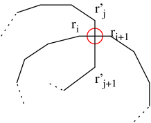
Figure 1: A regular intersection between lines (circled).

We recall the definition of multiplication $*$ in ${{\mathcal{B}}}$ and relate to ‘pictures’ of partitions.

(2.1) Fix a dimension $d>0$. Given an ordered list $r=(r^{1},r^{2},...,r^{l})$ of points in ${\mathbb{R}}^{d}$, let

$$(r)=\bigcup_{i=1}^{l-1}[r^{i},r^{i+1}]$$

where $[r^{i},r^{i+1}]\subset{\mathbb{R}}^{d}$ is the straight line between these points.

A line or polygonal path in the plane ${\mathbb{R}}^{2}$ is a subset of form $(r)$ such that each point $r^{i}$ lies in at most two of the straight lines.

(2.2) Let $R\subset{\mathbb{R}}^{2}$ be a rectangle, with frame $\partial R$ and interior $(R)=R\setminus\partial R$. A set of lines is regular in $R$ if:
(R1) each line $(r)\subset R$ touches $\partial R$ only if $r^{1}\neq r^{l}$ and then only at its end-points $r^{1},r^{l}$;
(R2) the point-list $r^{1},r^{2},...,r^{l}$ of each line has no intersection with any other line. See Fig. 1.

(2.3) Remark. Given a regular set of lines $D$, consider the subset $p(D)$ of $R$ defined by $D$. Note that we can recover the points of $D$ from $d=p(D)$ except for those points $r^{i}$ that are colinear with their neighbours $r^{i-1},r^{i+1}$. Note that colinearity is not a generic condition. The fibre $p^{-1}(d)$ of regular sets of lines over $d$ includes a representative $D^{\prime}$ in which no line has an $i$ with $r^{i-1},r^{i},r^{i+1}$ colinear. The fibre consists of sets obtained by inserting such colinear points in lines.

Note that $d$ completely determines $D$ up to such inserted colinear points.

(2.4) A Brauer picture $d$ of a partition $p$ in $J(n,m)$ is a rectangle $R\subset{\mathbb{R}}^{2}$ with $n$ points (called ‘vertices’) labeled $1,2,...,n$ on the northern edge, and $m$ on the southern edge (as in Figure 2); and a subset of $R$ consisting of a regular set of lines $(r)$ in $R$ as follows. Each line is either a loop ($r^{1}=r^{l}$) or else connects vertices pairwise in accordance with the pairs in $p$.

Figure 2: A picture of $\{\{3,1\},\{5,3^{\prime}\},\{4,2\},\{2^{\prime},1^{\prime}\}\}\in J(5,3)$. N.B. Drawings of piecewise-smooth approximations to piecewise-linear embeddings are safe to use here, provided that crossings remain manifestly transversal.

See Fig.2 and Fig.3 for examples. Remark: As far as physically drawn figures are concerned, piecewise linear and piecewise smooth lines are effectively indistinguishable, by [Moise77, §6] for example.

(2.5) Note that the construction ensures a well-defined map $\pi$ from pictures to partitions: for each $i\in V^{n}_{m}$ the line from $i$ in $d$ may be followed unambiguously to the other end; and one takes a line with end-points $i,j$ to $\{i,j\}$.

(2.6) For $p\in J(n,m)$ write $[p]$ for the set of pictures $d$ such that $\pi(d)=p$. Note that every $[p]$ is non-empty. Write $\#(d)$ for the number of loops in picture $d$.

(2.7) Recall $\delta\in k$. We extend the $\pi$-map to $\Pi(d)=\delta^{\#(d)}\pi({d})\in kJ(m,n)$.

For $d$ a picture let $\hat{d}$ denote $d$ with all loops removed. Thus $\Pi(d)=\delta^{\#(d)}\Pi(\hat{d})$.

(2.8) Consider pictures $d_{1}$ for $p_{1}\in J(m,n)$ and $d_{2}$ for $p_{2}\in J(n,q)$.

We have not specified exactly where the $n$ vertices lie on the southern frame of $R$ in $d_{1}$ (or indeed where the southern frame lies in ${\mathbb{R}}^{2}$), but it will be clear that there are representative pictures of $p_{1},p_{2}$ for which the $n$ vertices from $d_{1}$ match up with the $n$ from $d_{2}$. These pictures can then be stacked (with $d_{1}$ over $d_{2}$) so that the $n$ vertex sets in each ‘factor’ coincide. Note that the concatenation is again a Brauer picture. It is denoted by $d_{1}\,|\,d_{2}$.

Note then (1) that $d_{1}|d_{2}$ can be seen as a picture of an element of $kJ(m,q)$;
(2) that if $d_{2}$ and $d_{3}$ also stack then

$$(d_{1}|d_{2})|d_{3}=d_{1}|(d_{2}|d_{3})$$ (1)

2.2 The Brauer partition category ${\mathcal{B}}$

Given a set $p$ of symbols, let $p^{\prime}$ be the set obtained by adding primes to symbols in $p$ (note that this can work recursively). For example $\{\{1,2\},\{3,2^{\prime}\},\{1^{\prime},3^{\prime}\}\}^{\prime}=\{\{1^{\prime},2^{\prime}\},\{3^{\prime},2^{\prime\prime}\},\{1^{\prime\prime},3^{\prime\prime}\}\}$.

(2.9) Let $p_{1}\in J(m,n)$ and $p_{2}\in J(n,q)$. Now form $p_{1}\cup p_{2}^{\prime}$. Note that $p_{1}$ and $p_{2}^{\prime}$ may not be quite disjoint in general. When a primed pair in $p_{1}$ meets the corresponding unprimed pair from $p_{2}$ the union ‘flattens’ this to a single pair. Note each single-primed element appears twice (or once if flattened) and others once. Consider a maximal chain $\{a_{0},a_{1}\},\{a_{1},a_{2}\},...,\{a_{k-1},a_{k}\}$ in $p_{1}\cup p_{2}^{\prime}$. The chain is either all primed, and $a_{0}=a_{k}$ or $k=1$; or else $\{a_{0},a_{k}\}$ lies in $\underline{m}\cup\underline{q}^{\prime\prime}$ (to which we may apply $i^{\prime\prime}\leadsto i^{\prime}$ to obtain an element of $\underline{m}\cup\underline{q}^{\prime}$). In this way $p_{1}\cup p_{2}^{\prime}$ determines an element $p_{1}.p_{2}$ of $J(m,q)$; and also a number $\#$ of all-primed ‘closed’ chains. Define

$$p_{1}*p_{2}=\;\delta^{\#}p_{1}.p_{2}\;\in kJ(m,q).$$

Note that if $d_{i}\in[p_{i}]$ and $d_{1}|d_{2}$ then
(I) each maximal chain above corresponds to vertices in a line component of $d_{1}|d_{2}$.
(II) the pair $\{a_{0},a_{k}\}$ corresponds to the vertices at the ends of the line component of $d_{1}|d_{2}$. Thus the image in $\pi(d_{1}|d_{2})$ if $a_{0}\neq a_{k}$ is $\{a_{0},a_{k}\}$ (more precisely $\{a_{0},a_{k}\}$ with any $i^{\prime\prime}\leadsto i^{\prime}$).

(2.10) From the notes (I,II) in (2.2) we have, independently of the choice of pictures,

$$p_{1}*p_{2}=\Pi(d_{1}\,|\,d_{2}).$$

For example, from Figure 4 (ignoring the red line for now)

$$\{\{4^{\prime},2\},\{3,5^{\prime}\},\{1,3^{\prime}\},\{1^{\prime},2^{\prime}\}\}*\{\{2,1\},\{4,5\},\{1^{\prime},3\}\}\;=\;\delta\{\{3,2\},\{1,1^{\prime}\}\}\;\in kJ(3,1)\ .$$

Note we use the convention that a picture $d_{1}$ for $p_{1}\in J(m,n)$ has $m$ (resp. $n$) points on its northern (southern) edge. Thus $d_{1}\,|\,d_{2}$ is the concatenation of $d_{1}$ on top of $d_{2}$.

(2.11) Theorem.

[KadarMartinYu] Composition $*$ is associative. This defines the category ${\mathcal{B}}$.

Proof.

By the points (I,II) in (2.2) above we may obtain $p_{1}*p_{2}$ from $d_{1}|d_{2}$ (independently of the choices of these pictures). Existence of constructs of form $d_{1}|(d_{2}|d_{3})$ will be evident. Associativity follows since $(d_{1}|d_{2})|d_{3}=d_{1}|(d_{2}|d_{3})$. (Alternatively we may stay with the initial machinery of (2.2) and simply introduce more primes. The pictures can be seen as bookkeeping the primes.) ∎

(2.12) Define $\otimes:J(n,m)\times J(n^{\prime},m^{\prime})\rightarrow J(n+n^{\prime},m+m^{\prime})$ as the composition corresponding to side-by-side concatenation of pictures. Note the following.

(2.13) Lemma.

(I) The composition $\otimes$ makes ${\mathcal{B}}$ into a monoidal category.
(II) Let $w\in J(n,m)$ for some $n,m$, with $J(n,m)\hookrightarrow kJ(n,m)$ in the natural way. Then $p\otimes w=q\otimes w$ implies $p=q$. ∎

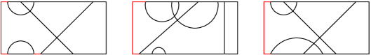
Figure 3: ‘Lowest-height’ pictures of elements of $J(4,4)$.

2.3 The subcategory ${\mathcal{J}}_{l}$ of category ${\mathcal{B}}$

The regularity property (R2) of a picture $d$ means that the number, and position, of crossings of lines in $d$ is well-defined. A path through a picture $d$ is a further line in $R$ that satisfies (R2).

Fix a picture $d$, let $x$ be a point in $d$, and consider all paths from $x$ to the left edge. Then ‘left-height’ $h_{d}(x)$ is the minimum number of crossings with lines of the picture among such paths.

The left-height $h(d)$ of a picture $d$ is the maximum $h_{d}(x)$ of all crossing points $x$ of lines in $d$; or, if there are no crossings, then $h(d)=-1$.

For $p\in J(n,m)$ let $h(p)$ denote the minimum $h(d)$ among pictures in $[p]=\{d:\pi(d)=p\}$. Define

$$J_{\leq l}(n,m)=\{p\in J(n,m)\;|\;h(p)\leq l\}$$

Define $[p]^{\prime}$ as the subset of $[p]$ of pictures of $p$ of the minimum height. That is,

$$[p]^{\prime}=\{d\in[p]\;|\;h(d)=h(p)\}.$$

See Fig.3 for examples of minimum height pictures.

As shown in [KadarMartinYu], $h(p_{1}*p_{2})\leq\max(h(p_{1}),(h(p_{2}))$. A consequence is the following.

(2.14) Theorem.

[KadarMartinYu] Category ${{\mathcal{B}}}$ has a subcategory ${\mathcal{J}}_{l}=({\mathbb{N}}_{0},kJ_{\leq l}(n,m),*)$. ∎

(2.15) Given a subset $S$ of a rectangle $R$, an alcove of $S$ is a connected component of $R\setminus S$.

(2.16) Remark. Let $d\in[p]$. Note that alcoves of $d$ have well-defined left-height. Note that the left-heights of the intervals of the frame of $R$ are determined by $p$, and are otherwise independent of $d$.

Proof: Note that there exist paths $w$ from the left edge of $R$ to points on $\partial R$ such that $w$ lies in a neighbourhood of $\partial R$. Note (e.g. from the Jordan Curve Theorem) that there are such paths that have the lowest number of crossings. By construction two pictures $d,d^{\prime}\in[p]$ are close to identical in a neighbourhood of $\partial R$. In particular there are paths to points on $\partial R$ that lie in such a neighbourhood; have the lowest number of crossings; and that have the same number of crossings in $d$ and $d^{\prime}$. ∎

2.4 The blob category ${\mathfrak{b}}$

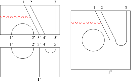
Figure 4: A left-exposed line is a part of a left-exposed line after concatenation.

Figure 5: An illustrative blob picture.

Now we recall the blob category [MartinSaleur94a]. Note that for $p\in J_{-1}(m,n)$ a pictures $d$ in $[p]^{\prime}$ has no crossings. Thus for each pair $v$ in $p$ the corresponding line $l_{v}$ in $d\in[p]^{\prime}$ has the property that every point $x$ on $l_{v}$ has the same value of $h_{d}(x)$. Furthermore this $h_{d}(l_{v})=h_{d}(x)$ depends only on $v$ in $p$ and not on $d$. Thus $v$ has a well-defined $h(v)=h_{d}(l_{v})$. A left-exposed pair in $p\in J_{-1}(m,n)$ is a pair $v$ with $h(v)=0$. (That is, there exists a path from the left edge of $R$ to $l_{v}$, which path does not intersect any line of $d$, for $d\in[p]^{\prime}$. The line $l_{v}$ is literally left-exposed.)

(2.17) Lemma.

Let $p_{1}\in J_{-1}(m,n)$ and $p_{2}\in J_{-1}(n,q)$. Let $d_{i}\in[p_{i}]^{\prime}$. Let $v$ be a left-exposed pair in $p_{1}$ or $p_{2}$ and let $l_{v}$ be the corresponding line in $d_{i}$. Then the line $l$ in $d_{1}\,|\,d_{2}$ containing $l_{v}$ has $h_{d}(l)=0$.

Proof.

A path connecting the line $l_{v}$ to the left edge without intersection in $d_{1}$ or $d_{2}$ also connects the line in $d_{1}|d_{2}$ which contains $l_{v}$ to the left edge without intersection (cf. Fig.4). ∎

(2.18) For $p\in J_{-1}(m,n)$ let $S^{L}_{p}$ denote the subset of left-exposed pairs. Define

$${{\mathsf{J}}^{\bullet}}(m,n)\;=\;\{(p,s)\,|\,p\in J_{-1}(m,n),\;s\subset S^{L}_{p}\}$$ (2)

(2.19) Let $(p_{1},s_{1})\in{{\mathsf{J}}^{\bullet}}(m,n)$ and $(p_{2},s_{2})\in{{\mathsf{J}}^{\bullet}}(n,q)$. Recall $p_{1}.p_{2}$ and $p_{1}*p_{2}$ from (2.2). Define $\overline{s_{1}s_{2}}$ to be the set of those pairs $\{a_{0},a_{k}\}$ in $p_{1}.p_{2}$, from chains $\{a_{0},a_{1}\},\{a_{1},a_{2}\},\dots,\{a_{k-1},a_{k}\}$ where at least one pair comes (in the obvious sense) from $s_{1}$ or $s_{2}$. Define $\#$ as the number of closed chains with no pair from $s_{1},s_{2}$, and $\#^{\prime}$ as the number of remaining closed chains.

We fix $\delta,\delta^{\prime}\in k$ and define the composition $\circ:{{\mathsf{J}}^{\bullet}}(m,n)\times{{\mathsf{J}}^{\bullet}}(n,q)\to k{{\mathsf{J}}^{\bullet}}(m,q)$ by

$$(p_{1},s_{1})\circ(p_{2},s_{2})=\;\delta^{\#}\delta^{\prime\#^{\prime}}(p_{1}.p_{2},\overline{s_{1}s_{2}}).$$

(2.20) Theorem.

Fix a commutative ring $k$ and $\delta,\delta^{\prime}\in k$. Then ${\mathfrak{b}}=(\mathbb{N}_{0},k{{\mathsf{J}}^{\bullet}}(n,m),\circ)$ is a category.

Proof.

We require to prove associativity of the product, and this follows analogously to (2.2) and (2.11). Again the bookkeeping of extra primes may be seen from suitable pictures.

(2.21) A picture with blobs is a pair $(d,b)$ where $d$ is a picture in the sense of (1); and $b$ is a set of points (called blobs) in the interiors of lines of $d$. We require that each blob lies in exactly one line (if $d\in[p]^{\prime}$ with $p\in J_{-1}$ then lines here are non-crossing and this is automatic).

(2.22) Given a picture with blobs $(d,b)$ such that $h_{d}(x\in b)=0$ we define

$$\pi^{\prime}:(d,b)\mapsto(\pi(d),s(b))\;\in{{\mathsf{J}}^{\bullet}}(m,n)$$

where $\pi$ is as in (2) and $s(b)$ is the set of pairs associated to the lines decorated by $b$.

(2.23) An element $(p,s)\in{{\mathsf{J}}^{\bullet}}(m,n)$ can be represented by a pair $(d,b)$, where $d$ is a no-loop picture of $p$; and $b$ consists of at least one point in the interior of each line of $d$ corresponding to a pair in $s$. See Fig.5.

For an example note that Figure 5 is a picture $(d,\{P_{1},P_{2},P_{3}\})$ for an element

$$(p,s)=(\{\{2^{\prime},1^{\prime}\},\{9,10\},\{3,4\},\{7^{\prime},5\},\{1,2\},\{8,8^{\prime}\},\{3^{\prime},6^{\prime}\},\{5^{\prime},4^{\prime}\},\{6,7\}\},\;\{\{5,7^{\prime}\},\{1,2\},\{6^{\prime},3^{\prime}\}\})$$

$\in{{\mathsf{J}}^{\bullet}}(10,8)$. The blobs $P_{i},i=1,2,3$ are mapped to the pairs $\{2,1\}$, $\{5,7^{\prime}\}$, $\{6^{\prime},3^{\prime}\}$ respectively.

(2.24) Define

$$\Pi(d,b)\;\;:=\;\;\delta^{\#(d,b)}\delta^{\prime\#^{\prime}(d,b)}\;\pi^{\prime}({d},{b})\;\;\in k{{\mathsf{J}}^{\bullet}}(m,n),$$

where $\#(d,b)$ (respectively $\#^{\prime}(d,b)$) is the number of loops without (respectively with) blobs.

Let $d_{i}\in[p_{i}]^{\prime}$ and $(d_{i},b_{i})$ be no-loop pictures with appropriate blobs (hereafter we just write $d_{i}$, including blobs). By Lem.2.17 the concatenated picture $d_{1}\,|\,d_{2}$ is a picture of some $p\in J(m,q)$ plus possible loops and blobs. By an argument similar to (2.2) we have, independently of choices,

$$(p_{1},s_{1})\circ(p_{2},s_{2})=\;\Pi(d_{1}|d_{2}).$$

Existence of constructs of form $d_{1}|(d_{2}|d_{3})$ will again be evident. Since again $d_{1}|(d_{2}|d_{3})=(d_{1}|d_{2})|d_{3}$ we are done. ∎

(2.24.1) Corollary.

The End sets $k{{\mathsf{J}}^{\bullet}}(m,m)$ have the structure of an associative algebra.

We may denote these algebras by $J^{\bullet\,\delta,\delta^{\prime}}_{m}$, or simply ${\mathfrak{b}}_{m}$, indicating the fixed parameters from $k$ in the definition of the multiplication only when needed for clarity.

Figure 6: (a) The basis ${{\mathsf{J}}^{\bullet}}(1,1)$.                     (b) The basis ${{\mathsf{J}}^{\bullet}}(2,2)$.

(2.25) Examples. Consider Fig.6(a,b). Applying the rules of multiplication we have e.g., $1e=e1=ee=e$, $\;f_{1}^{2}=\delta f_{1}$, $f_{2}^{2}=\delta^{\prime}f_{2}$, $f_{2}f_{1}=f_{2}f_{3}=\delta^{\prime}f_{1}$, $f_{6}f_{1}=f_{6}f_{3}=f_{3}$ and so on.

2.5 Generators and relations

(2.26) Theorem.

[MartinSaleur94a, Martin0706] Consider the algebra defined by generators $U^{e}=\{e,U_{1},U_{2},...,U_{n-1}\}$ and relations
$\tau^{\prime}=\{\mbox{ $U_{i}^{2}=\delta U_{i}$, $U_{i}U_{i\pm 1}U_{i}=U_{i}$, $U_{i}U_{j}=U_{j}U_{i}$, $j\neq i\pm 1$, $ee=e$, $U_{1}eU_{1}=\delta^{\prime}U_{1}$, $U_{i}e=eU_{i}$, $i>1$ }\}$. (I) The map

$$U_{i}\mapsto\{\underbrace{\{\{1,1^{\prime}\}\{2,2^{\prime}\},...,\{i,i+1\},\{i^{\prime},i+1^{\prime}\},...,\{n,n^{\prime}\}\}}_{p},\underbrace{\emptyset}_{s}\}$$

$$e\mapsto\{\underbrace{\{\{1,1^{\prime}\},\{2,2^{\prime}\},...,\{n,n^{\prime}\}\}}_{p},\underbrace{\{\{1,1^{\prime}\}\}}_{s}\}\hskip 72.26999pt$$

extends to an algeba isomorphism $k\langle U^{e}\rangle/\tau^{\prime}\cong{\mathfrak{b}}_{n}$.
(II) Every element of the partition basis ${{\mathsf{J}}^{\bullet}}(n,n)$ can be expressed as a word in these generators. In particular $(p,s)\in{{\mathsf{J}}^{\bullet}}(n,n)$ can be expressed as a word in which $e$ appears as a factor $|s|$ times. ∎

2.6 Generator algebras $B_{l,m,n}$ and spin chain Physics

The original motivation for the blob algebra [MartinSaleur94a] was to study XXZ spin chains (and other related spin chains [AlcarazQuispell, LiebMattis66]) with various boundary conditions via representation theory. In the simplest formulation (see [PasquierSaleur90, Levy91, MartinSaleur94a] for details) one notes that there are boundary conditions for which the $n$-site XXZ chain Hamiltonian may be expressed in the form

$$H=\sum_{i=1}^{n-1}U_{i}$$

where $U_{i}$ acts on $(\mathbb{C}^{2})^{n}$ by

$$U_{i}=1_{2}\otimes 1_{2}\otimes...\otimes\left(\begin{array}[]{cccc}0\\ &q&1\\ &1&q^{-1}\\ &&&0\end{array}\right)\otimes 1_{2}\otimes...\otimes 1_{2}$$

It is known that these matrices give a faithful representation of the Temperley–Lieb algebra. In this sense the algebra controls the spectrum of $H$. A centraliser algebra is $U_{q}sl_{2}$, and so this can equivalently be seen as controlling the spectrum.

There are several reasons for wanting to generalise away from this particular choice of boundary conditions. For example: (1) periodic boundary conditions may be desirable for reasons of computability or to minimise boundary effects at finite size. (2) one may be interested in critical bulk physics in the presence of a doped boundary. (3) one may be interested in physics on the surface of a bulk system (typically perhaps a 2D surface in 3D, but modelled more simply by a thickened finite interval at the end of an infinite line).

The generalisation required for the periodic case requires quite delicate tuning — see [MartinSaleur94a]. But the simplest form of such generalisation is simply to modify the first or last operator in the chain:

$$H^{\prime}=U^{\prime}_{0}+\sum_{i=1}^{n-1}U_{i}$$

where $U^{\prime}_{0}$ acts only on the first tensor factor (and then of course to take the thermodynamic limit) [Levy91]. The corresponding extension of the Temperley–Lieb algebra is covered by the blob algebra. Another challenge is to dope with a more complex operator at the boundary. Algebraically this generalisation can get difficult quite quickly. A version which at least lies within the Brauer algebra is to have a Temperley–Lieb chain with some permutation operators at the end. That is, one first considers the Brauer algebra $B_{n}$ as the algebra generated by its sub-symmetric group and Temperley–Lieb Coxeter generator elements

$$B_{n}=\langle\sigma_{i},U_{i}\;:\;i=1,2,...,n-1\rangle$$ (3)

Note that this is not a minimal generating set. For example, all but one $U_{i}$ can be discarded.

(2.27) Trivially one can then define for each $n$ a ‘Coxeter subalgebra’

$$B_{l,m,n}=\langle\sigma_{i},\;:\;i=1,2,...,l-1,\;\;U_{i},\;:\;i=m,m+1,...,n-1\rangle$$

It is clear that various values of $l,m$ reduce to known cases. For example if $m>l$ then we just have a product of $S_{l}$ and $T_{n-m}$. So the interesting cases are $m\leq l$. …

The Hamiltonians for such systems have been considered [Bondersan], but in the present work we focus on the abstract algebraic aspects.

It is clear that $B_{l,1,n}\hookrightarrow{\mathcal{J}}_{l,n}$; and that $B_{2,2,n}\hookrightarrow{{\mathcal{J}}_{0,n}^{1}}$. It is conjectured that these inclusions are isomorphisms. … And in this spirit we can ask about a geometrical and categorical characterisation of $B_{l,l,n}$.

(2.28) The disk order on elements of $\{1,2,...,m\}\cup\{1^{\prime},2^{\prime},...,n^{\prime}\}$ is given by renumbering $i^{\prime}\mapsto m+n+1-i$. In our convention for pictures of $p$ this is clockwise order on the topological marked disk $R$ — see fig.7. For $\{i,j\}$ a pair in $p\in J(m,n)$, with $i<j$ in the disk order, we understand by $[i,j]$ the interval from $i$ to $j$ with respect to the disk order.

Figure 7: Disk order on vertices.

3 The subcategory ${\mathcal{J}}_{i-1}^{i}$ of ${\mathcal{J}}_{i-1}$

(3.1) Let $S$ be a totally ordered set and $p$ a partition of $S$ into pairs (we have in mind the disk order as in (2.6)). Via the total order, the restriction of $p$ to any two pairs induces a partition of $\{1,2,3,4\}$. The set of such partitions is $\{\{\{1,3\},\{2,4\}\},\;\{\{1,2\},\{3,4\}\},\;\{\{1,4\},\{2,3\}\}\}$.

A pair in $p$ is crossing in $p$ if there is another pair in $p$ such that the partition induced by the restriction of $p$ to these two pairs is $\{\{1,3\},\{2,4\}\}$.

Remark: The point of this terminology is that if the total order is the disk order then in every picture $d$ of $p$ the line for the ‘crossing’ pair must cross another line. (This follows from the Jordan curve theorem [Moise77].)

3.1 The crossing number $\chi_{p}$ of a partition

Figure 8: Schematic for removing a line self-crossing in a picture.

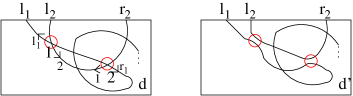
Figure 9: Cancellation: Small neighbourhoods of two crossings of two lines in a picture $d\in[p]$ modified such that the resulting picture satisfies $d^{\prime}\in[p]$ with two fewer crossings.

(3.2) We denote the number of crossings of a picture $d\in[p]$ by $\#^{c}(d)$

(3.3) Let $p$ be a Brauer partition and let $\{\{l_{1},r_{1}\},\{l_{2},r_{2}\}\}$ be two pairs in $p$. Note by the Jordan Curve Theorem that if precisely one of $l_{2},r_{2}$ lies in the (disk)-interval from $l_{1}$ to $r_{1}$ then a picture of $p$ must have at least one crossing of the lines corresponding to these two pairs — we say the two pairs ‘cross’. We thus have a lower bound on the number of crossings in a picture $d$ of $p$:

$$\#\geq\chi_{p}$$

where

$$\chi_{p}=\sum_{\{\{l_{1},r_{1}\},\{l_{2},r_{2}\}\}\subset p}\delta(\{\{l_{1},r_{1}\},\{l_{2},r_{2}\}\})$$

where the sum is over pairs of pairs and $\delta(-)$ is 1 if they cross and zero otherwise.

(3.4) Lemma.

Consider $p\in J(n,m)$. There exist pictures $d$ of $p$ achieving the minimum $\#^{c}(d)=\chi_{p}$.

Proof.

First consider a picture $d\in[p]$ with a line self-crossing. Then note from (1) that removing the open segment of the line corresponding to the loop starting and ending at the self-crossing produces another picture $d^{\circ}$, such that $\pi(d^{\circ})=\pi(d)$. Next, see Fig.9. It shows that whenever there are two crossings of the same two lines in $d\in[p]$ these crossing neighbourhoods may be ‘cancelled’ to make $d^{\prime}\in[p]$ with two fewer crossings. ∎