Convergence of a Stochastic Gradient Method with Momentum for Non-Smooth Non-Convex Optimization

Abstract

Stochastic gradient methods with momentum are widely used in applications and at the core of optimization subroutines in many popular machine learning libraries. However, their sample complexities have not been obtained for problems beyond those that are convex or smooth. This paper establishes the convergence rate of a stochastic subgradient method with a momentum term of Polyak type for a broad class of non-smooth, non-convex, and constrained optimization problems. Our key innovation is the construction of a special Lyapunov function for which the proven complexity can be achieved without any tuning of the momentum parameter. For smooth problems, we extend the known complexity bound to the constrained case and demonstrate how the unconstrained case can be analyzed under weaker assumptions than the state-of-the-art. Numerical results confirm our theoretical developments.

1 Introduction

We study the stochastic optimization problem

$$\underset{x\in\mathcal{X}}{\mathop{\mathrm{minimize}}}\,f(x):=\mathbb{E}_{P}[f(x;S)]=\int_{\mathcal{S}}f(x;s)dP(s),$$ (1)

where $S\sim P$ is a random variable; $f(x;s)$ is the instantaneous loss parameterized by $x$ on a sample $s\in\mathcal{S}$; and $\mathcal{X}\subseteq\mathbb{R}^{n}$ is a closed convex set. In this paper, we move beyond convex and/or smooth optimization and consider $f$ that belongs to a broad class of non-smooth and non-convex functions called $\rho$-weakly convex, meaning that

$$x\mapsto f(x)+\rho\left\|{x}\right\|_{2}^{2}\,\,\,\mbox{is convex}.$$

This function class is very rich and important in optimization [39, 47]. It trivially includes all convex functions, all smooth functions with Lipschitz continuous gradient, and all additive composite functions of the two former classes. More broadly, it includes all compositions of the form

$$f(x)=h(c(x)),$$ (2)

where $h:\mathbb{R}^{m}\to\mathbb{R}$ is convex and $L_{h}$-Lipschitz and $c:\mathbb{R}^{n}\to\mathbb{R}^{m}$ is a smooth map with $L_{c}$-Lipschitz Jacobian. Indeed, the composite function $f=h\circ c$ is then weakly convex with $\rho=L_{h}L_{c}$ [11]. Some representative applications in this problem class include nonlinear least squares [10], robust phase retrieval [13], Robust PCA [6], robust low rank matrix recovery [7], optimization of the Conditional Value-at-Risk [40], graph synchronization [44], and many others.

Stochastic optimization algorithms for solving (1), based on random samples $S_{k}$ drawn from $P$, are of fundamental importance in many applied sciences [4, 43]. Since the introduction of the classical stochastic (sub)gradient descent method (SGD) in [38], several modifications of SGD have been proposed to improve its practical and theoretical performance. A notable example is the use of a momentum term to construct an update direction [24, 37, 42, 46, 45, 19]. The basis form of such a method (when $\mathcal{X}=\mathbb{R}^{n}$) reads:

$$x_{k+1} =x_{k}-\alpha_{k}z_{k}$$ (3a)

$$z_{k+1} =\beta_{k}g_{k+1}+(1-\beta_{k})z_{k},$$ (3b)

where $z_{k}$ is the search direction, $g_{k}$ is a stochastic subgradient; $\alpha_{k}$ is the stepsize, and $\beta_{k}\in(0,1]$ is the momentum parameter. For instance, the scheme (3) reduces to the stochastic heavy ball method (SHB) [37]:

$$x_{k+1} =x_{k}-\eta_{k}g_{k}+\lambda_{k}(x_{k}-x_{k-1}),$$

with $\eta_{k}=\alpha_{k}\beta_{k-1}$ and $\lambda_{k}=(1-\beta_{k-1})\alpha_{k}/\alpha_{k-1}$. Methods of this type enjoy widespread empirical success in large-scale convex and non-convex optimization, especially in training neural networks, where they have been used to produce several state-of-the-art results on important learning tasks, e.g., [29, 45, 25, 28].

Sample complexity, namely, the number of observations $S_{0},\ldots,S_{K}$ required to reach a desired accuracy $\epsilon$, has been the most widely adapted metric for evaluating the performance of stochastic optimization algorithms. Although sample complexity results for the standard SGD on problems of the form (1) have been obtained for convex and/or smooth problems [30, 18], much less is known in the non-smooth non-convex case [8]. The problem is even more prevalent in momentum-based methods as there is virtually no known complexity results for problems beyond those that are convex or smooth.

1.1 Related work

As many applications in modern machine learning and signal processing cannot be captured by convex models, (stochastic) algorithms for solving non-convex problems have been studied extensively. Below we review some of the topics most closely related to our work.

Stochastic weakly convex minimization   Earlier works on this topic date back to Nurminskii who showed subsequential convergence to stationary points for the subgradient method applied to deterministic problems [34]. The work [41] proposes a stochastic gradient averaging-based method and shows the first almost sure convergence for this problem class. Basic sufficient conditions for convergence of stochastic projected subgradient methods is established in [15]. Thanks to the recent advances in statistical learning and signal processing, the problem class has been reinvigorated with several new theoretical results and practical applications (see, e.g., [13, 12, 9, 8] and references therein). In particular, based on the theory of non-convex differential inclusions, almost sure convergence is derived in [14] for a collection of model-based minimization strategies, albeit no rates of convergence are given. An important step toward non-asymptotic convergence of stochastic methods is made in [9]. There, the authors employ a proximal point technique for which they can show the sample complexity $O(1/\epsilon^{2})$ with a certain stationarity measure. Later, the work [8] shows that the (approximate) proximal point step in [9] is not necessary and establishes the similar complexity for a class of model-based methods including the standard SGD. We also note that there has been a large volume of works in smooth non-convex optimization, e.g., [18, 19].

Stochastic momentum for non-convex functions   Optimization algorithms based on momentum averaging techniques go back to Polyak [36] who proposed the heavy ball method. In [31], Nesterov introduced the accelerated gradient method and showed its optimal iteration complexity for the minimization of smooth convex functions. In the last few decades, research on accelerated first-order methods has exploded both in theory and in practice [3, 33, 5]. The effectiveness of such techniques in the deterministic context has inspired researchers to incorporate momentum terms into stochastic optimization algorithms [37, 41, 46, 45, 19]. Despite evident success, especially, in training neural networks [29, 45, 25, 50, 28], the theory for stochastic momentum methods is not as clear as its deterministic counterpart (cf. [22]). As a result, there has been a growing interest in obtaining convergence guarantees for those methods under noisy gradients [27, 22, 49, 16, 19]. In non-convex optimization, almost certain convergence of Algorithm (3) for smooth and unconstrained problems is derived in [42]. Under the bounded gradient hypothesis, the convergence rate of the same algorithm has been established in [49]. The work [21] obtains the complexity of a gradient averaging-based method for constrained problems. In [19], the authors study a variant of Nesterov acceleration and establish a similar complexity for smooth and unconstrained problems, while for the constrained case, a mini-batch of samples at each iteration is required to guarantee convergence.

1.2 Contributions

Minimization of weakly convex functions has been a challenging task, especially for stochastic problems, as the objective is neither smooth nor convex. With the recent breakthrough in [8], this problem class has been the widest one for which provable sample complexity of the standard SGD is known. It is thus intriguing to ask whether such a result can also be obtained for momentum-based methods. The work in this paper aims to address this question. To that end, we make the following contributions:

• We establish the sample complexity of a stochastic subgradient method with momentum of Polyak type for a broad class of non-smooth, non-convex, and constrained optimization problems. Concretely, using a special Lyapunov function, we show the complexity $O(1/\epsilon^{2})$ for the minimization of weakly convex functions. The proven complexity is attained in a parameter-free and single time-scale fashion, namely, the stepsize and the momentum constant are independent of any problem parameters and they have the same scale with respect to the iteration count. To the best of our knowledge, this is the first complexity guarantee for a stochastic method with momentum on non-smooth and non-convex problems.

• We also study the sample complexity of the considered algorithm for smooth and constrained optimization problems. Note that even in this setting, no complexity guarantee of SGD with Polyak momentum has been established before. Under a bounded gradient assumption, we obtain a similar $O(1/\epsilon^{2})$ complexity without the need of forming a batch of samples at each iteration, which is commonly required for constrained non-convex stochastic optimization [20]. We then demonstrate how the unconstrained case can be analyzed without the above assumption.

Interestingly, the stated result is achieved in the regime where $\beta$ can be as small as $O(1/\sqrt{K})$, i.e., one can put much more weight to the momentum term than the fresh subgradient in a search direction. This complements the complexity of SGD attained as $\beta\to 1$. Note that the worst-case complexity $O(1/\epsilon^{2})$ is unimprovable in the smooth and unconstrained case [1].

2 Background

In this section, we first introduce the notation and then provide the necessary preliminaries for the paper.

For any $x,y\in\mathbb{R}^{n}$, we denote by $\left\langle x,y\right\rangle$ the Euclidean inner product of $x$ and $y$. We use $\left\|{\cdot}\right\|_{2}$ to denote the Euclidean norm. For a closed and convex set $\mathcal{X}$, ${\mathop{\Pi}}_{\mathcal{X}}$ denotes the orthogonal projection onto $\mathcal{Z}$, i.e., $y={\mathop{\Pi}}_{\mathcal{X}}\left(x\right)$ if $y\in\mathcal{X}$ and $\left\|{y-x}\right\|_{2}=\min_{z\in\mathcal{X}}\left\|{z-x}\right\|_{2}$; $\mathsf{I}_{\mathcal{X}}(\cdot)$ denotes the indicator function of $\mathcal{X}$, i.e., $\mathsf{I}_{\mathcal{X}}(x)=0$ if $x\in\mathcal{X}$ and $+\infty$ otherwise. Finally, we denote by $\mathcal{F}_{k}:=\sigma(S_{0},\ldots,S_{k})$ the $\sigma$-field generated by the first $k+1$ random variables $S_{0},\ldots,S_{k}$.

For a function $f:\mathbb{R}^{n}\to\mathbb{R}\cup\{+\infty\}$, the Fréchet subdifferential of $f$ at $x$, denoted by $\partial f(x)$, consists of all vectors $g\in\mathbb{R}^{n}$ such that

$$f(y)\geq f(x)+\left\langle g,y-x\right\rangle+o(\left\|{y-x}\right\|)\,\,\,\mbox{as}\,\,\,y\to x.$$

The Fréchet and conventional subdifferentials coincide for convex functions, while for smooth functions $f$, $\partial f(x)$ reduces to the gradient $\{\nabla f(x)\}$. A point $x\in\mathbb{R}^{n}$ is said to be stationary for problem (1) if $0\in\partial{f(x)+\partial\mathsf{I}_{\mathcal{X}}(x)}$.

The following lemma collects standard properties of weakly convex functions [47].

Lemma 2.1 (Weak convexity).

Let $f:\mathbb{R}^{n}\to\mathbb{R}\cup\{+\infty\}$ be a $\rho$-weakly convex function. Then the following hold:

1.

For any $x,y\in\mathbb{R}^{n}$ with $g\in\partial f(x)$, we have

$$f(y)\geq f(x)+\left\langle g,y-x\right\rangle-\frac{\rho}{2}\left\|{y-x}\right\|_{2}^{2}.$$

2.

For all $x,y\in\mathbb{R}^{n}$, $\alpha\in[0,1]$, and $z=\alpha x+(1-\alpha)y$:

$$f(z) \leq\alpha f(x)+(1-\alpha)f(y)+\frac{\rho\alpha(1-\alpha)}{2}\left\|{x-y}\right\|_{2}^{2}.$$

Weakly convex functions admit an implicit smooth approximation through the Moreau envelope:

$$f_{\lambda}(x)=\inf_{y\in\mathbb{R}^{n}}\left\{f(y)+\frac{1}{2\lambda}\left\|{x-y}\right\|_{2}^{2}\right\}.$$ (4)

For small enough $\lambda$, the point achieving $f_{\lambda}(x)$ in (4), denoted by ${\mathop{\mathrm{prox}}}_{\lambda f}\left(x\right)$, is unique and given by:

$${\mathop{\mathrm{prox}}}_{\lambda f}\left(x\right)=\mathop{\mathrm{argmin}}_{y\in\mathbb{R}^{n}}\left\{f(y)+\frac{1}{2\lambda}\left\|{x-y}\right\|_{2}^{2}\right\}.$$ (5)

The lemma below summarizes two well-known properties of the Moreau envelope and its associated proximal map [26].

Lemma 2.2 (Moreau envelope).

Suppose that $f:\mathbb{R}^{n}\to\mathbb{R}\cup\{+\infty\}$ is a $\rho$-weakly convex function. Then, for a fixed parameter $\lambda^{-1}\geq 2\rho$, the following hold:

1.

$f_{\lambda}$ is $\mathcal{C}^{1}$-smooth with the gradient given by

$$\nabla f_{\lambda}(x)=\lambda^{-1}\left(x-{\mathop{\mathrm{prox}}}_{\lambda f}\left(x\right)\right).$$

2.

$f_{\lambda}$ is $\lambda^{-1}$-smooth, i.e., for all $x,y\in\mathbb{R}^{n}$:

$$\big{|}f_{\lambda}(y)-f_{\lambda}(x)-\left\langle\nabla f_{\lambda}(x),y-x\right\rangle\big{|}\leq\frac{1}{2\lambda}\left\|{x-y}\right\|_{2}^{2}.$$

Failure of stationarity test   A major source of difficulty in convergence analysis of non-smooth optimization methods is the lack of a controllable stationarity measure. For smooth functions, it is natural to use the norm of the gradient as a surrogate for near stationarity. However, this rule does not make sense in the non-smooth case, even if the function is convex and its gradient existed at all iterates. For example, the convex function $f(x)=|x|$ has $\left\|{\nabla f(x)}\right\|_{2}=1$ at each $x\neq 0$, no mater how close $x$ is to the stationary point $x=0$.

To circumvent this difficulty, we adopt the techniques pioneered in [8] for convergence of stochastic methods on weakly convex problems. More concretely, we rely on the connection of the Moreau envelope to (near) stationarity: For any $x\in\mathbb{R}^{n}$, the point $\hat{x}={\mathop{\mathrm{prox}}}_{\lambda F}\left(x\right)$, where $F(x)=f(x)+\mathsf{I}_{\mathcal{X}}(x)$, satisfies:

$$\begin{cases}\left\|{x-\hat{x}}\right\|_{2}=\lambda\left\|{\nabla F_{\lambda}(x)}\right\|_{2},\\ \mathop{\mathrm{dist}}(0,\partial F(\hat{x}))\leq\left\|{\nabla F_{\lambda}(x)}\right\|_{2}.\end{cases}$$ (6)

Therefore, a small gradient $\left\|{\nabla F_{\lambda}(x)}\right\|_{2}$ implies that $x$ is close to a point $\hat{x}\in\mathcal{X}$ that is near-stationary for $F$. Note that $\hat{x}$ is just a virtual point, there is no need to compute it.

3 Algorithm and convergence analysis

We assume that the only access to $f$ is through a stochastic subgradient oracle. In particular, we study algorithms that attempt to solve problem (1) using i.i.d. samples $S_{0},S_{1},\ldots,S_{K}\stackrel{{\scriptstyle\mathrm{iid}}}{{\sim}}P$.

Assumption A (Stochastic oracle).

Fix a probability space $(\mathcal{S},\mathcal{F},P)$. Let $S$ be a sample drawn from $P$ and $f^{\prime}(x,S)\in\partial f(x,S)$. We make the following assumptions:

(A1)

For each $x\in\mathop{\mathrm{dom}}(f)$, we have

$$\mathbb{E}_{P}\left[f^{\prime}(x,S)\right]\in\partial f(x).$$

(A2)

There exists a real $L>0$ such that for all $x\in\mathcal{X}$:

$$\mathbb{E}_{P}\left[\left\|{f^{\prime}(x,S)}\right\|_{2}^{2}\right]\leq L^{2}.$$

The above assumptions are standard in stochastic optimization of non-smooth functions (see, e.g., [30, 8]).

Algorithm   To solve problem (1), we use an iterative procedure that starts from $x_{0}\in\mathcal{X}$, $z_{0}\in\partial f(x_{0},S_{0})$ and generates sequences of points $x_{k}\in\mathcal{X}$ and $z_{k}\in\mathbb{R}^{n}$ by repeating the following steps for $k=0,1,2,\ldots$:

$$x_{k+1} =\mathop{\mathrm{argmin}}_{x\in\mathcal{X}}\left\{\left\langle z_{k},x-x_{k}\right\rangle+\frac{1}{2\alpha}\left\|{x-x_{k}}\right\|_{2}^{2}\right\}$$ (7a)

$$z_{k+1} =\beta g_{k+1}+(1-\beta)\frac{x_{k}-x_{k+1}}{\alpha},$$ (7b)

where $g_{k+1}\in\partial f(x_{k+1},S_{k+1})$. When $\mathcal{X}=\mathbb{R}^{n}$, this algorithm reduces to the procedure (3). For a general convex set $\mathcal{X}$, this scheme is known as the iPiano method in the smooth and deterministic setting [35]. For simplicity, we refer to Algorithm 7 as stochastic heavy ball (SHB).

Throughout the paper, we will frequently use the following two quantities:

$$p_{k}=\frac{1-\beta}{\beta}\left(x_{k}-x_{k-1}\right)\,\,\mbox{and}\,\,\,d_{k}=\frac{1}{\alpha}\left(x_{k-1}-x_{k}\right).$$

Before detailing our convergence analysis, we note that most proofs of $O(1/\epsilon^{2})$ sample complexity for subgradient-based methods rely on establishing an iterate relationship on the form (see, e.g., [30, 8, 18]):

$$\mathbb{E}[V_{k+1}]\leq\mathbb{E}[V_{k}]-\alpha\,\mathbb{E}[e_{k}]+\alpha^{2}C^{2},$$ (8)

where $e_{k}$ denotes some stationarity measure such as $f(\cdot)-f^{\star}$ for convex and $\left\|{\nabla f(\cdot)}\right\|_{2}^{2}$ for smooth (possibly non-convex) problems, $V_{k}$ are certain Lyapunov functions, $\alpha$ is the stepsize, and $C$ is some constant. Once (8) is given, a simple manipulation results in the desired complexity provided that $\alpha$ is chosen appropriately. The case with decaying stepsize can be analyzed in the same way with minor adjustments. We follow the same route and identify a Lyapunov function that allows to establish relation (8) for the quantity $\left\|{\nabla F_{\lambda}(\cdot)}\right\|_{2}$ in (6).

Since our Lyapunov function is nontrivial, we shall build it up through a series of key results. We start by presenting the following lemma, which quantifies the averaged progress made by one step of the algorithm.

Lemma 3.1.

Let Assumptions (A1)–(A2) hold. Let $\beta=\nu\alpha$ for some constant $\nu>0$ such that $\beta\in(0,1]$. Let $x_{k}$ be generated by procedure (7). It holds for any $k\in\mathbb{N}$ that

$$(1-\beta)f(x_{k})+\mathbb{E}\left[\frac{\nu}{2}\left\|{p_{k+1}}\right\|_{2}^{2}|\mathcal{F}_{k-1}\right] \leq(1-\beta)f(x_{k-1})+\frac{\nu}{2}\left\|{p_{k}}\right\|_{2}^{2}-\alpha\,\mathbb{E}\left[\left\|{d_{k+1}}\right\|_{2}^{2}|\mathcal{F}_{k-1}\right]$$

$$\hskip 12.80365pt+\alpha^{2}\left(\frac{\rho(1-\beta)}{2}+\nu\right)L^{2}.$$ (9)

Proof.

See Appendix A. ∎

In view of (8), the lemma shows that the quantity $\mathbb{E}[\left\|{d_{k}}\right\|_{2}^{2}]$ can be made arbitrarily small. However, this alone is not sufficient to show convergence to stationary points. Nonetheless, we shall show that a small $\mathbb{E}[\left\|{d_{k}}\right\|_{2}^{2}]$ indeed implies a small (averaged) value of the norm of the Moreau envelope defined at a specific point. Toward this goal, we first need to detail the points $x$ and $\hat{x}$ in (6). It seems that taking the most natural candidate $x=x_{k}$ is unlikely to produce the desired result. Instead, we rely on the following iterates:

$$\bar{x}_{k}:=x_{k}+\frac{1-\beta}{\beta}\left(x_{k}-x_{k-1}\right),$$

and construct corresponding virtual reference points:

$$\hat{x}_{k}=\mathop{\mathrm{argmin}}_{x\in\mathbb{R}^{n}}\left\{F(x)+\frac{1}{2\lambda}\left\|{x-\bar{x}_{k}}\right\|_{2}^{2}\right\},$$

for $\lambda<1/\rho$. By Lemma 2.2, $\nabla F_{\lambda}(\bar{x}_{k})=\lambda^{-1}(\bar{x}_{k}-\hat{x}_{k})$, where $F_{\lambda}(\cdot)$ is the Moreau envelope of $F(\cdot)=f(\cdot)+\mathsf{I}_{\mathcal{X}}(\cdot)$.

With these definitions, we can now state the next lemma.

Lemma 3.2.

Assume the same setting of Lemma 3.1. Let $\lambda>0$ be such that $\lambda^{-1}\geq 2\rho$. Let $\xi=(1-\beta)/\nu$ and define the function:

$$V_{k} =F_{\lambda}(\bar{x}_{k})+\frac{\nu\xi^{2}}{4\lambda^{2}}\left\|{p_{k}}\right\|_{2}^{2}+\frac{\alpha\xi^{2}}{2\lambda^{2}}\left\|{d_{k}}\right\|_{2}^{2}+\left(\frac{(1-\beta)\xi^{2}}{2\lambda^{2}}+\frac{\xi}{\lambda}\right)f(x_{k-1}).$$ (10)

Then, for any $k\in\mathbb{N}$,

$$\mathbb{E}\left[V_{k+1}|\mathcal{F}_{k-1}\right]\leq V_{k}-\frac{\alpha}{2}\left\|{\nabla F_{\lambda}(\bar{x}_{k})}\right\|_{2}^{2}+\frac{\gamma\alpha^{2}L^{2}}{2\lambda},$$ (11)

where $\gamma={\xi^{2}({\rho(1-\beta)}/{2}+\nu)}/{\lambda}+{\rho\xi}/{2}+1$.

The proof of this lemma is rather involved and can be found in Appendix B. Lemma 3.2 has established a relation akin to (8) with the Lyapunov function $V_{k}$ defined in (10). We can now use standard analysis to obtain our sample complexity.

Theorem 1.

Let Assumptions (A1)-(A2) hold. Let $k^{*}$ be sampled uniformly at random from $\{0,\ldots,K\}$. Let $f^{\star}=\inf_{x\in\mathcal{X}}f(x)$ and denote $\Delta=f(x_{0})-f^{\star}$. If we set $\alpha=\frac{\alpha_{0}}{\sqrt{K+1}}$ and $\nu=1/\alpha_{0}$ for some real $\alpha_{0}>0$, then under the same setting of Lemma 3.2:

$$\mathbb{E}\left[\left\|{\nabla F_{\lambda}(\bar{x}_{k^{*}})}\right\|_{2}^{2}\right]\leq 2\cdot\frac{\gamma_{1}\Delta+\frac{\gamma L^{2}}{2\lambda}}{\alpha_{0}\sqrt{K+1}},$$ (12)

where $\gamma\leq\rho^{2}\alpha_{0}^{2}+3\rho\alpha_{0}+1$ and $\gamma_{1}\leq 2\rho^{2}\alpha_{0}^{2}+2\rho\alpha_{0}+1$. Furthermore, if $\alpha_{0}$ is set to $1/\rho$, we obtain

$$\mathbb{E}\left[\left\|{\nabla F_{1/(2\rho)}(\bar{x}_{k^{*}})}\right\|_{2}^{2}\right]\leq 10\cdot\frac{\rho\Delta+L^{2}}{\sqrt{K+1}}.$$

Proof.

Taking the expectation on both sides of (11) and summing the result over $k=0,\ldots,K$ yield

$$\mathbb{E}\left[V_{K+1}\right]\leq{V_{0}}-\frac{\alpha_{0}}{2\sqrt{K+1}}\sum_{k=0}^{K}\mathbb{E}\left[\left\|{\nabla F_{\lambda}(\bar{x}_{k})}\right\|_{2}^{2}\right]+\frac{\gamma L^{2}\alpha_{0}^{2}}{2\lambda}.$$

Let $\gamma_{1}={1+(1-\beta)\xi^{2}}/({2\lambda^{2}})+{\xi}/{\lambda}$, the left-hand-side of the above inequality can be lower-bounded by $\gamma_{1}f^{\star}$. Using the facts that $F_{\lambda}(x_{0})\leq f(x_{0})$ and $x_{-1}=x_{0}$, we get $V_{0}\leq\gamma_{1}f(x_{0})$. Consequently,

$$\mathbb{E}\left[\left\|{\nabla F_{\lambda}(\bar{x}_{k^{*}})}\right\|_{2}^{2}\right]\leq 2\cdot\frac{\gamma_{1}\Delta+\frac{\gamma L^{2}\alpha_{0}^{2}}{2\lambda}}{\alpha_{0}\sqrt{K+1}},$$

where the last expectation is taken with respect to all random sequences generated by the method and the uniformly distributed random variable $k^{*}$. Note that $\nu=1/\alpha_{0}$, $\xi=(1-\beta)/\nu$, and $1-\beta\leq 1$. Thus, letting $\lambda=1/(2\rho)$, the constants $\gamma$ and $\gamma_{1}$ can be upper-bounded by $\rho^{2}\alpha_{0}^{2}+3\rho\alpha_{0}+1$ and $2\rho^{2}\alpha_{0}^{2}+2\rho\alpha_{0}+1$, respectively. Therefore, if we let $\alpha_{0}=1/\rho$, we arrive at

$$\mathbb{E}\left[\left\|{\nabla F_{1/(2\rho)}(\bar{x}_{k^{*}})}\right\|_{2}^{2}\right]\leq 10\cdot\frac{\rho\Delta+L^{2}}{\sqrt{K+1}},$$

as desired. ∎

Some remarks regarding Theorem 1 are in order:

i) The choice $\nu=1/\alpha_{0}$ is just for simplicity; one can pick any constant such that $\beta=\nu\alpha\in(0,1]$. Note that the stepsize used to achieve the rate in (12) does not depend on any problem parameters. Once $\alpha$ is set, the momentum parameter selection is completely parameter-free. Since both $\alpha$ and $\beta$ scale like $O(1/\sqrt{K})$, Algorithm 7 can be seen as a single time-scale method [21, 42]. Such methods contrast those that require at least two time-scales to ensure convergence. For example, stochastic dual averaging for convex optimization [48] requires one fast scale $O(1/K)$ for averaging the subgradients, and one slower scale $O(1/\sqrt{K})$ for the stepsize. To show almost sure convergence of SHB for smooth and unconstrained problems, the work [22] requires that both the stepsize and the momentum parameter tend to zero but the former one must do so at a faster speed.

ii) To some extent, Theorem 1 supports the use of a small momentum parameter such as $\beta=0.1$ or $\beta=0.01$, which corresponds to the default value $1-\beta=0.9$ in PyTorch or the smaller $1-\beta=0.99$ suggested in [23]. Indeed, the theorem allows to have $\beta$ as small as $O(1/\sqrt{K})$, i.e., one can put much more weight to the momentum term than the fresh subgradient and still preserve the complexity. Recall also that SHB reduces to SGD as $\beta\to 1$, which also admits a similar complexity. It is thus quite flexible to set $\beta$, without sacrificing the worst-case complexity. We refer to [22, Theorem 2] for a similar discussion in the context of almost sure convergence on smooth problems.

iii) In view of (6), the theorem indicates that $\bar{x}_{k}$ is nearby a near-stationary point $\hat{x}_{k}$. Since $\bar{x}_{k}$ may not belong to $\mathcal{X}$, it is thus more preferable to have the similar guarantee for the iterate $x_{k}$. Indeed, we have

$$\lambda^{-2}\left\|{x_{k}-\hat{x}_{k}}\right\|_{2}^{2} \leq 2\lambda^{-2}\left\|{\bar{x}_{k}-\hat{x}_{k}}\right\|_{2}^{2}+2\lambda^{-2}\left\|{x_{k}-\bar{x}_{k}}\right\|_{2}^{2}$$

$$=2\left\|{\nabla F_{\lambda}(\bar{x}_{k})}\right\|_{2}^{2}+2\lambda^{-2}\left\|{x_{k}-\bar{x}_{k}}\right\|_{2}^{2}$$

$$=2\left\|{\nabla F_{\lambda}(\bar{x}_{k})}\right\|_{2}^{2}+2\lambda^{-2}\xi^{2}\left\|{d_{k}}\right\|_{2}^{2}.$$

Since both terms on the right converge at the rate $O(1/\sqrt{K})$, it immediately translates into the same guarantee for the term on the left, as desired.

In summary, we have established the convergence rate $O(1/\sqrt{K})$ or, equivalently, the sample complexity $O(1/\epsilon^{2})$ of SHB for the minimization of weakly convex functions.

4 Extension to smooth non-convex functions

In this section, we study the convergence property of Algorithm (7) for the minimization of $\rho$-smooth functions:

$$\left\|{\nabla f(x)-\nabla f(x)}\right\|_{2}\leq\rho\left\|{x-y}\right\|_{2},\,\,\,\forall x,y\in\mathop{\mathrm{dom}}f.$$

Note that $\rho$-smooth functions are automatically $\rho$-weakly convex. In this setting, it is more common to replace Assumption (A2) by the following.

Assumption (A3). There exists a real $\sigma>0$ such that for all $x\in\mathcal{X}$:

$$\mathbb{E}\left[\left\|{f^{\prime}(x,S)-\nabla f(x)}\right\|_{2}^{2}\right]\leq\sigma^{2}.$$

Deriving convergence rates of stochastic schemes with momentum for non-convex functions under Assumption (A3) can be quite challenging. Indeed, even in unconstrained optimization, previous studies often need to make the assumption that the true gradient is bounded, i.e., $\left\|{\nabla f(x)}\right\|_{2}\leq G$ for all $x\in\mathbb{R}^{n}$ (see, e.g., [49, 22]). This assumption is strong and does not hold even for quadratic convex functions. It is more realistic in constrained problems, for example when $\mathcal{X}$ is compact, albeit the constant $G$ could then be large.

Our objective in this section is twofold: First, we aim to extend the convergence results of SHB in the previous section to smooth optimization problems under Assumption (A3). Note that even in this setting, the sample complexity of SHB has not been established before. The rate is obtained without the need of forming a batch of samples at each iteration, which is commonly required for constrained non-convex stochastic optimization [19, 20]. Second, for unconstrained problems, we demonstrate how to achieve the same complexity without the bounded gradient assumption above.

Let $h(x)=\frac{1}{2}\left\|{x}\right\|_{2}^{2}+\mathsf{I}_{\mathcal{X}}(x)$ and let $h^{*}(z)$ be its convex conjugate. Our convergence analysis relies on the function:

$$\varphi_{k}=h^{*}(x_{k}-\alpha z_{k})-\frac{1}{2}\left\|{x_{k}}\right\|_{2}^{2}+\alpha\left\langle x_{k},z_{k}\right\rangle.$$ (13)

The use of this function is inspired by [41]. Roughly speaking, $\varphi_{k}$ is the negative of the optimal value of the function on the RHS of (7a), and hence, $\varphi_{k}\geq 0$ for all $k$. This function also underpins the analysis of the dual averaging scheme in [32].

The following result plays a similar role as Lemma 3.1.

Lemma 4.1.

Let Assumptions (A1) and (A3) hold. Let $\alpha\in(0,1/\rho)$ and $\beta=\nu\alpha$ for some constant $\nu>0$ such that $\beta\in(0,1]$. Let $\alpha\in\left(0,1/(4\rho)\right]$ and $\xi=(1-\beta)/\nu$, and define the function:

$$W_{k}=2f(x_{k})+\frac{\varphi_{k}}{\nu\alpha^{2}}+\frac{\xi}{2}\left\|{d_{k}}\right\|_{2}^{2}.$$

Then, it holds for any $k\in\mathbb{N}$ that

$$\mathbb{E}\left[W_{k+1}|\mathcal{F}_{k}\right] \leq W_{k}-\alpha\left\|{d_{k+1}}\right\|_{2}^{2}+4\nu\alpha^{2}\sigma^{2}.$$ (14)

Proof.

Since the proof is rather technical, we defer details to Appendix C and sketch only the main arguments here.

By smoothness of $h^{*}$, weak convexity of $f$ and the optimality condition for the update formula (7a) we get

$$\mathbb{E}\left[f(x_{k+1})+\frac{\varphi_{k+1}}{\nu\alpha^{2}}\Big{|}\mathcal{F}_{k}\right] \leq f(x_{k})+\frac{\varphi_{k}}{\nu\alpha^{2}}-(\alpha-\frac{\rho\alpha^{2}}{2})\left\|{d_{k+1}}\right\|_{2}^{2}+\frac{1}{2\nu}\mathbb{E}\left[\left\|{z_{k}-z_{k+1}}\right\|_{2}^{2}|\mathcal{F}_{k}\right].$$

The proof of this relation can be found in Lemma C.1. The preceding inequality admits very useful properties as we have terms that form a telescoping sum, and the constant associated with $\left\|{d_{k+1}}\right\|_{2}^{2}$ has the right order-dependence on the stepsize. However, we still have a remaining term $\left\|{z_{k}-z_{k+1}}\right\|_{2}^{2}$. Thus, in view of relation (8), our next strategy is to bound this term in a way that still keeps all the favourable features described above, and at the most introduces an additional term of order $O(\alpha^{2}\sigma^{2})$. As shown in Lemma C.2, we can establish the following inequality

$$\mathbb{E}\left[\frac{1}{2\nu}\left\|{z_{k+1}-z_{k}}\right\|_{2}^{2}|\mathcal{F}_{k}\right] \leq f(x_{k})-f(x_{k+1})+\frac{\xi}{2}\left\|{d_{k}}\right\|_{2}^{2}-\frac{\xi}{2}\left\|{d_{k+1}}\right\|_{2}^{2}$$

$$\hskip 12.80365pt-\left(\alpha-\frac{\alpha^{3}\rho^{2}+3\rho\alpha^{2}}{2}\right)\left\|{d_{k+1}}\right\|_{2}^{2}+4\nu\alpha^{2}\sigma^{2}.$$

Now, (14) follows immediately from combining the two previous inequalities and the fact that $\alpha\in\left(0,1/(4\rho)\right]$. ∎

We remark that Lemma 4.1 does not require the bounded gradient assumption and readily indicates the convergence rate $O(1/\sqrt{K})$ for $\mathbb{E}[\left\|{d_{k}}\right\|_{2}^{2}]$. However, to establish the rate for $\mathbb{E}[\left\|{\nabla F_{\lambda}(\bar{x}_{k})}\right\|_{2}^{2}]$, we need to impose such an assumption in the theorem below. Nonetheless, the assumption is much more realistic in this setting than the unconstrained case.

Theorem 2.

Let Assumptions (A1) and (A3) hold. Assume further that $\left\|{\nabla f(x)}\right\|_{2}\leq G$ for all $x\in\mathcal{X}$. Let $k^{*}$, $\bar{x}_{k^{*}}$, $\lambda$, $\Delta$, $\gamma$, and $\gamma_{1}$ be defined as in Theorem 1. If we set $\alpha=\frac{\alpha_{0}}{\sqrt{K+1}}$ and $\nu=1/\alpha_{0}$ for some real $\alpha_{0}>0$, then

$$\mathbb{E}\left[\left\|{\nabla F_{\lambda}(\bar{x}_{k^{*}})}\right\|_{2}^{2}\right]\leq 2\cdot\frac{\gamma_{1}\Delta+{\gamma(\sigma^{2}+G^{2})}/({2\lambda})}{\alpha_{0}\sqrt{K+1}}.$$

Furthermore, if $\alpha_{0}$ is set to $1/\rho$, we obtain

$$\mathbb{E}\left[\left\|{\nabla F_{1/(2\rho)}(\bar{x}_{k^{*}})}\right\|_{2}^{2}\right]\leq 10\cdot\frac{\rho\Delta+\sigma^{2}+G^{2}}{\sqrt{K+1}}.$$

Proof.

The proof is a verbatim copy of that of Theorem 1 with $L^{2}$ replaced by $\sigma^{2}+G^{2}$; see Appendix D. ∎

Some remarks are in order:

i) To the best of our knowledge, this is the first convergence rate result of a stochastic (or even deterministic) method with Polyak momentum for smooth, non-convex, and constrained problems.

ii) The algorithm enjoys the same single time-scale and parameter-free properties as in the non-smooth case.

iii) The rate in the theorem readily translates into an analogous estimate for the norm of the so-called gradient mapping $\mathcal{G}_{1/\rho}$, which is commonly adapted in the literature, e.g., [20]. This is because for $\rho$-smooth functions [11]:

$$\left\|{\mathcal{G}_{1/\rho}(x)}\right\|_{2}\leq\frac{3}{2}(1+\frac{1}{\sqrt{2}})\left\|{\nabla F_{1/(2\rho)}(x)}\right\|_{2},\,\,\,\forall x\in\mathbb{R}^{n}.$$

Since the bounded gradient assumption is rather restrictive in the unconstrained case, our final result shows how the desired complexity can be attained without this assumption.

Theorem 3.

Let Assumptions (A1) and (A3) hold. Let $\lambda^{-1}\in(3\rho/2,2\rho]$. Let $k^{*}$ be sampled uniformly at random from $\{-1,\ldots,K-1\}$. If we set $\alpha=\frac{\alpha_{0}}{\sqrt{K+1}}$ and $\nu=1/\alpha_{0}$, where $\alpha_{0}\in(0,1/(4\rho)]$, then under the same setting of Lemma 4.1:

$$\mathbb{E}\left[\left\|{\nabla F_{\lambda}(\bar{x}_{k^{*}})}\right\|_{2}^{2}\right]\leq c\cdot\frac{(1+2\alpha_{0}^{2}/\lambda^{2})\Delta+\frac{(1+{8\alpha_{0}}/{\lambda})\sigma^{2}\alpha_{0}^{2}}{2\lambda}}{\alpha_{0}\sqrt{K+1}},$$

where $c={2\lambda^{-1}}/{(2\lambda^{-1}-3\rho)}$. Furthermore, let $\lambda=1/(2\rho)$, we obtain

$$\mathbb{E}\left[\left\|{\nabla F_{1/(2\rho)}(\bar{x}_{k^{*}})}\right\|_{2}^{2}\right]\leq 4\cdot\frac{\left(1+{8\rho^{2}\alpha_{0}^{2}}\right)\Delta+{(\rho+16\alpha_{0}\rho^{2})}\sigma^{2}\alpha_{0}^{3}}{\alpha_{0}\sqrt{K+1}}.$$

Proof.

See Appendix E. ∎

It should be mentioned that a similar result has been attained very recently in [21] using a different analysis, albeit no sample complexity is given for the non-smooth case. It is still an open question if one can preserve the complexity in Theorem 2 without the bounded gradient hypothesis.

5 Numerical evaluations

In this section, we perform experiments to validate our theoretical developments and to demonstrate that despite sharing the same worst-case complexity, SHB can be better in terms of speed and robustness to problem and algorithm parameters than SGD.

We consider the robust phase retrieval problem [13, 14]: Given a set of $m$ measurements $(a_{i},b_{i})\in\mathbb{R}^{n}\times\mathbb{R}$, the phase retrieval problem seeks for a vector $x^{\star}$ such that $\left\langle a_{i},x^{\star}\right\rangle^{2}\approx b_{i}$ for most $i=1,\ldots,m$. Whenever the problem is corrupted with gross outliers, a natural exact penalty form of this (approximate) system of equations yields the minimization problem:

$$\mathop{\mathrm{minimize}}_{x\in\mathbb{R}^{n}}\frac{1}{m}\sum_{i=1}^{m}\big{|}\left\langle a_{i},x\right\rangle^{2}-b_{i}\big{|}.$$

This objective function is non-smooth and non-convex. In view of (2), it is the composition of the Lipschitz-continuous convex function $h(y)=\left\|{y}\right\|_{1}$ and the smooth map $c$ with $c_{i}(x)=\left\langle a_{i},x\right\rangle^{2}-b_{i}$. Hence, it is weakly convex.

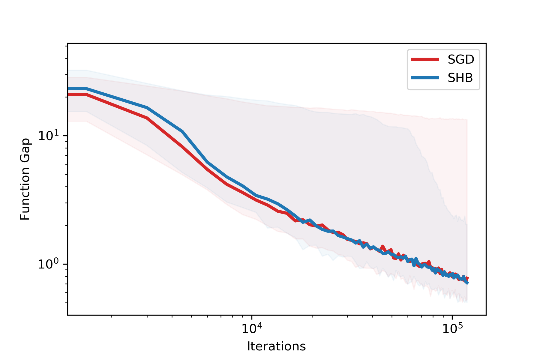
(a) $\kappa=10$, $\alpha_{0}=0.1$

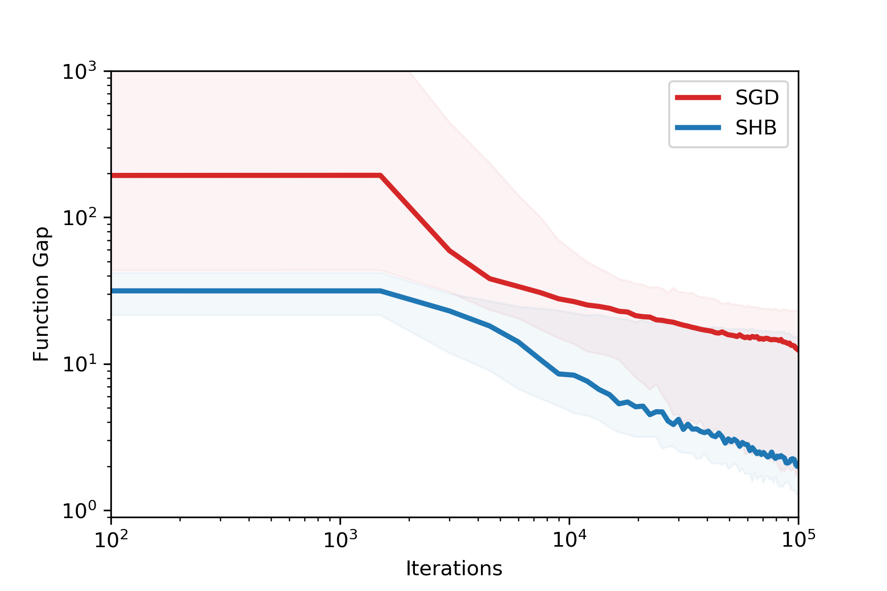
(b) $\kappa=10$, $\alpha_{0}=0.25$

(c) $\kappa=1$, $\alpha_{0}=0.1$

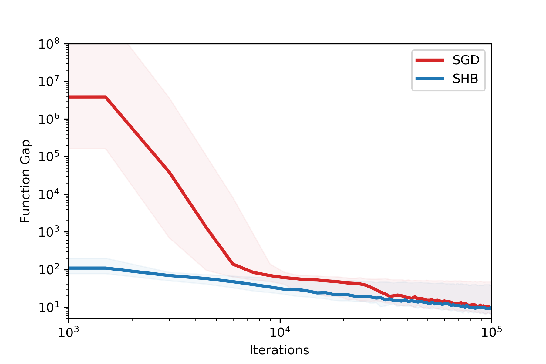
(d) $\kappa=1$, $\alpha_{0}=0.15$

Figure 1: The function gap $f(x_{k})-f(x^{\star})$ versus iteration count for phase retrieval with $p_{\textrm{fail}}=0.2$, $\beta=10/\sqrt{K}$. For better visualization, in this plot we generated $x^{\star}$ with standard normal distributed elements.

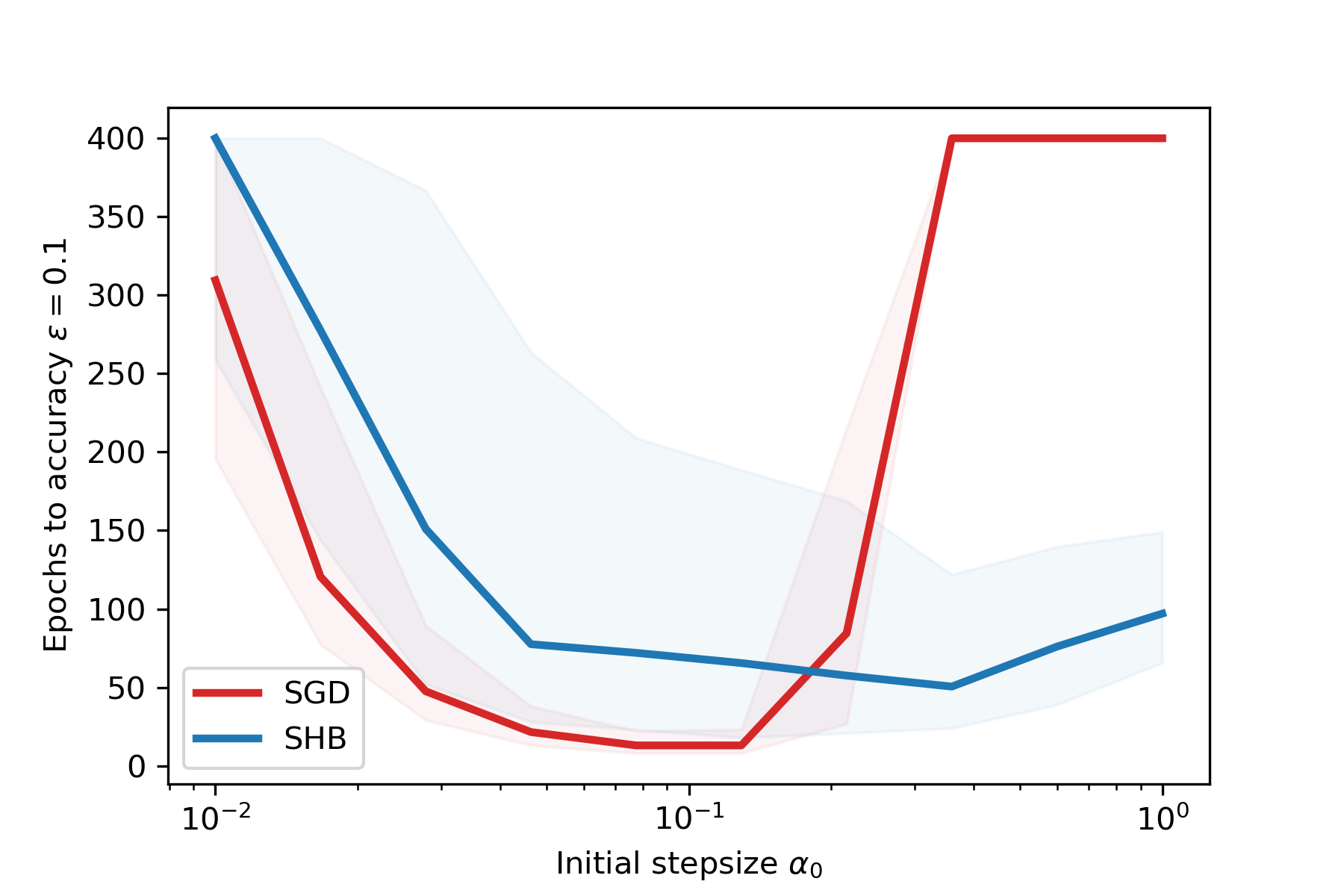
(a) $p_{\textrm{fail}}=0.3$, $\beta=1/\sqrt{K}$

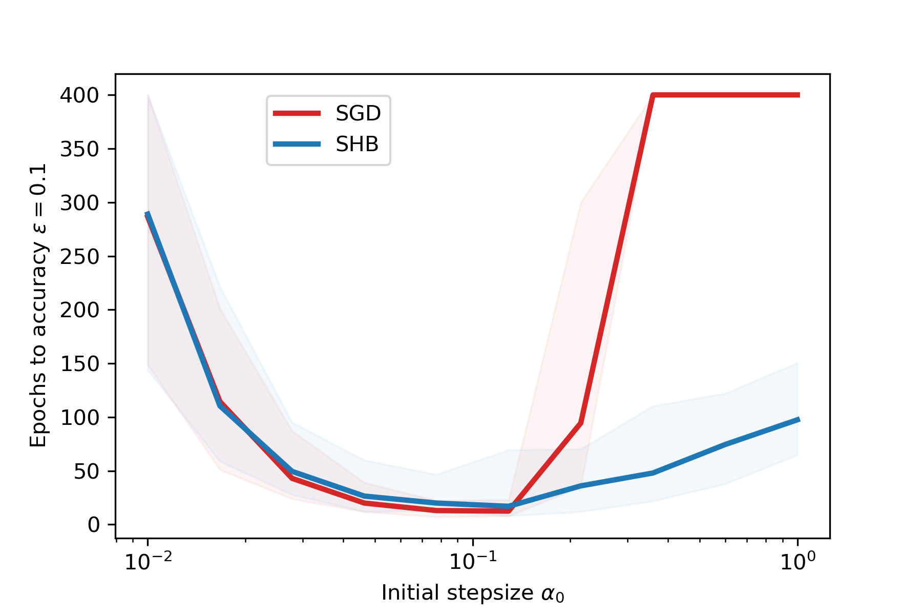
(b) $p_{\textrm{fail}}=0.3$, $\beta=1/\alpha_{0}/\sqrt{K}$

Figure 2: The number of epochs to achieve $\epsilon$-accuracy versus initial stepsize $\alpha_{0}$ for phase retrieval with $\kappa=10$.

(a) $p_{\textrm{fail}}=0.3$, $\beta=0.1$

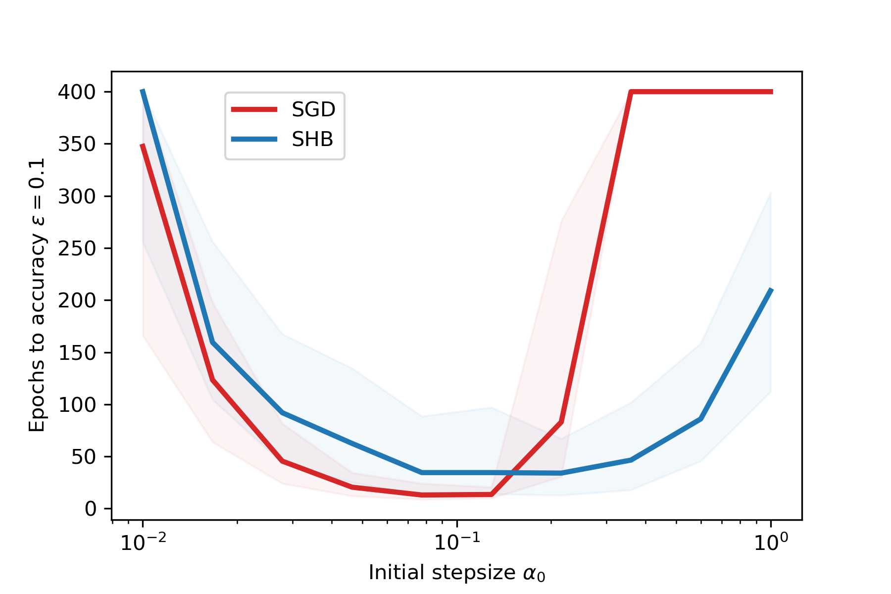
(b) $p_{\textrm{fail}}=0.3$, $\beta=0.01$

Figure 3: The number of epochs to achieve $\epsilon$-accuracy versus initial stepsize $\alpha_{0}$ for phase retrieval with $\kappa=10$ and popular choices of $\beta$.

In each experiment, we set $m=300$, $n=100$ and select $x^{\star}$ uniformly from the unit sphere. We generate $A$ as $A=QD$, where $Q\in\mathbb{R}^{m\times n}$ is a matrix with standard normal distributed entries, and $D$ is a diagonal matrix with linearly spaced elements between $1/\kappa$ and $1$, with $\kappa\geq 1$ playing the role of a condition number. The elements $b_{i}$ of the vector $b$ are generated as $b_{i}=\left\langle a_{i},x^{\star}\right\rangle^{2}+\delta\zeta_{i}$, $i=1,\ldots,m,$ where $\zeta_{i}\sim\mathcal{N}(0,25)$ models the corruptions, and $\delta\in\{0,1\}$ is a binary random variable taking the value $1$ with probability $p_{\textrm{fail}}$, so that $p_{\textrm{fail}}\cdot m$ measurements are corrupted. The algorithms are all randomly initialized at $x_{0}\sim\mathcal{N}(0,1)$. The stochastic subgradient is simply given as an element of the subdifferential of $g(x)=\big{|}\left\langle a,x\right\rangle^{2}-b\big{|}$:

$$\partial g(x)=2\left\langle a,x\right\rangle a\cdot\begin{cases}\mathop{\mathrm{sign}}{(\left\langle a,x\right\rangle-b)}^{2}&\mbox{if}\,\,\left\langle a,x\right\rangle^{2}\neq b,\\ [-1,1]&\mbox{otherwise}.\end{cases}$$

In each of our experiments, we set the stepsize as $\alpha_{k}=\alpha_{0}/\sqrt{k+1}$, where $\alpha_{0}$ is an initial stepsize. We note that this stepsize can often make a little faster progress (for both SGD and SHB) at the beginning of the optimization process than the constant one $\alpha_{k}=\alpha_{0}/\sqrt{K+1}$. However, after a few iterations, both of them yield very similar results and will not change the qualitative aspects of our plots in any way. We also refer $m$ stochastic iterations as one epoch (pass over the data). Within each individual run, we allow the considered stochastic methods to perform $K=400m$ iterations. We conduct 50 experiments for each stepsize and report the median of the so-called epochs-to-$\epsilon$-accuracy; the shaded areas in each plot cover the 10th to 90th percentile of convergence times. Here, the epoch-to-$\epsilon$-accuracy is defined as the smallest number of epochs $q$ required to reach $f(x_{m\cdot q})-f(x^{\star})\leq\epsilon$.

Figure 1 shows the function gap versus iteration count for different values of $\kappa$ and $\alpha_{0}$, with $p_{\textrm{fail}}=0.2$, $\beta=10/\sqrt{K}$. It is evident that SHB converges with a theoretically justified parameter $\beta$ and is much less sensitive to problem and algorithm parameters than the vanilla SGD. Note that the sensitivity issue of SGD is rather well documented; a slight change in its parameters can have a severe effect on the overall performance of the algorithm [30, 2]. For example, Fig. 1 shows that SGD exhibits a transient exponential growth before eventual convergence. This behaviour can occur even when minimizing the smooth quadratic function $\frac{1}{2}x^{2}$ [2, Example 2]. In contrast, SHB converges in all settings of the figure, suggesting that using a momentum term can help to improve the robustness of the standard SGD. This is expected as the update formula (3b) acts like a lowpass filter, averaging past stochastic subgradients, which may have stabilizing effect on the sequence $\{x_{k}\}$.

To further clarify this observation, in the next set of experiments, we test the sensitivity of SHB and SGD to the initial stepsize $\alpha_{0}$. Figure 2 shows the number of epochs required to reach $\epsilon$-accuracy for phase retrieval with $\kappa=10$ and $p_{\textrm{fail}}=0.3$. We can see that the standard SGD has good performance for a narrow range of stepsizes, while wider convergence range can be achieved with SHB.

Finally, it would be incomplete without reporting experiments for some of the most popular momentum parameters used by practitioners. Figure 3 shows a similar story to Fig. 2 for the parameter $1-\beta=0.9$ and $1-\beta=0.99$ as discussed in remark ii) after Theorem 1. This together with Fig. 2 demonstrates that SHB is able to find good approximate solutions for diverse values of the momentum constant over a wider (often significantly so) range of algorithm parameters than SGD.

6 Conclusion

Using a carefully constructed Lyapunov function, we established the first sample complexity results for the SHB method on a broad class of non-smooth, non-convex, and constrained optimization problems. The complexity is attained in a parameter-free fashion in a single time-scale. A notable feature of our results is that they justify the use of a large amount of momentum in search directions. We also improved some complexity results for SHB on smooth problems. Numerical results show that SHB exhibits good performance and low sensitivity to problem and algorithm parameters compared to the standard SGD.

Appendix A Proof of Lemma 3.1

First, we write the update formula of $x_{k+1}$ in (7) on a more compact form as:

$$x_{k+1} ={\mathop{\Pi}}_{\mathcal{X}}\left(x_{k}-\alpha z_{k}\right)$$ (15)

$$z_{k+1} =\beta g_{k+1}+(1-\beta)\frac{x_{k}-x_{k+1}}{\alpha}.$$ (16)

We have

$$\frac{1}{2}\left\|{\frac{1-\beta}{\beta}\left(x_{k+1}-x_{k}\right)}\right\|_{2}^{2}=\frac{1}{2\beta^{2}}\left\|{x_{k+1}-\left((1-\beta)x_{k}+\beta x_{k+1}\right)}\right\|_{2}^{2}.$$

Since $(1-\beta)x_{k}+\beta x_{k+1}\in\mathcal{X}$ and ${\mathop{\Pi}}_{\mathcal{X}}\left(\cdot\right)$ is nonexpansive, it holds that

$$\frac{1}{2}\left\|{\frac{1-\beta}{\beta}\left(x_{k+1}-x_{k}\right)}\right\|_{2}^{2} \leq\frac{1}{2\beta^{2}}\left\|{x_{k}-\alpha z_{k}-\left((1-\beta)x_{k}+\beta x_{k+1}\right)}\right\|_{2}^{2}$$

$$=\frac{1}{2}\left\|{x_{k}+\frac{1-\beta}{\beta}\left(x_{k}-x_{k-1}\right)-\alpha g_{k}-x_{k+1}}\right\|_{2}^{2}.$$ (17)

Next, we decompose the right-hand-side of the preceding inequality as

$$\frac{1}{2}\left\|{x_{k}+\frac{1-\beta}{\beta}\left(x_{k}-x_{k-1}\right)-\alpha g_{k}-x_{k+1}}\right\|_{2}^{2} =\frac{1}{2}\left\|{\frac{1-\beta}{\beta}\left(x_{k}-x_{k-1}\right)}\right\|_{2}^{2}$$

$$\hskip 12.80365pt+\frac{(1-\beta)\alpha}{\beta}\left\langle g_{k},x_{k-1}-x_{k}\right\rangle$$

$$\hskip 12.80365pt+\frac{1-\beta}{\beta}\left\langle x_{k}-x_{k-1},x_{k}-x_{k+1}\right\rangle+\alpha\left\langle g_{k},x_{k+1}-x_{k}\right\rangle$$

$$\hskip 12.80365pt+\frac{1}{2}\left\|{x_{k+1}-x_{k}}\right\|_{2}^{2}+\frac{\alpha^{2}}{2}\left\|{g_{k}}\right\|_{2}^{2}.$$ (18)

Let $p_{k}:=\frac{1-\beta}{\beta}\left(x_{k}-x_{k-1}\right)$, then by multiplying both sides of (A) by $\nu=\beta/\alpha>0$, together with (A) and the definition of $z_{k}$, we get

$$\frac{\nu}{2}\left\|{p_{k+1}}\right\|_{2}^{2} \leq\frac{\nu}{2}\left\|{p_{k}}\right\|_{2}^{2}+(1-\beta)\left\langle g_{k},x_{k-1}-x_{k}\right\rangle+\left\langle z_{k},x_{k+1}-x_{k}\right\rangle$$

$$\hskip 12.80365pt+\frac{\nu}{2}\left\|{x_{k+1}-x_{k}}\right\|_{2}^{2}+\frac{\nu\alpha^{2}}{2}\left\|{g_{k}}\right\|_{2}^{2}.$$ (19)

By the weak convexity of $f$ and Assumption (A1), it holds that

$$\mathbb{E}\left[\left\langle g_{k},x_{k-1}-x_{k}\right\rangle|\mathcal{F}_{k-1}\right] =\left\langle\mathbb{E}\left[g_{k}|\mathcal{F}_{k-1}\right],x_{k-1}-x_{k}\right\rangle$$

$$\leq f(x_{k-1})-f(x_{k})+\frac{\rho}{2}\left\|{x_{k}-x_{k-1}}\right\|_{2}^{2}.$$ (20)

Next using the optimality condition of $x_{k+1}$ in (7a):

$$\left\langle x_{k+1}-x_{k}+\alpha z_{k},x-x_{k+1}\right\rangle\geq 0\quad\mbox{for all}\,\,\,x\in\mathcal{X},$$ (21)

we deduce (by selecting $x=x_{k}\in\mathcal{X}$) that

$$\left\langle z_{k},x_{k+1}-x_{k}\right\rangle\leq-\alpha^{-1}\left\|{x_{k+1}-x_{k}}\right\|_{2}^{2}.$$ (22)

Therefore, by taking the conditional expectation in (A), combining the result with (A) and (22), and rearranging terms, we arrive at

$$(1-\beta)f(x_{k})+\mathbb{E}\left[\frac{\nu}{2}\left\|{p_{k+1}}\right\|_{2}^{2}|\mathcal{F}_{k-1}\right] \leq(1-\beta)f(x_{k-1})+\frac{\nu}{2}\left\|{p_{k}}\right\|_{2}^{2}$$

$$\hskip 12.80365pt-\left(\frac{1}{\alpha}-\frac{\nu}{2}\right)\mathbb{E}\left[\left\|{x_{k+1}-x_{k}}\right\|_{2}^{2}|\mathcal{F}_{k-1}\right]$$

$$\hskip 12.80365pt+\frac{(1-\beta)\rho}{2}\left\|{x_{k}-x_{k-1}}\right\|_{2}^{2}+\frac{\nu\alpha^{2}}{2}\mathbb{E}[\left\|{g_{k}}\right\|_{2}^{2}|\mathcal{F}_{k-1}].$$ (23)

Next, we show by induction that $\mathbb{E}[\left\|{z_{k}}\right\|_{2}^{2}|\mathcal{F}_{k-1}]\leq L^{2}\,\,\,\forall k\in\mathbb{N}$. Since $z_{0}\in\partial f(x_{0},S_{0})$, the base case follows directly from Assumption (A2). Suppose the hypothesis holds for $i=0,\ldots,k$, we have

$$\mathbb{E}[\left\|{z_{k+1}}\right\|_{2}^{2}|\mathcal{F}_{k}] =\mathbb{E}\left[\left\|{\beta g_{k+1}+(1-\beta)(x_{k}-x_{k+1})/{\alpha}}\right\|_{2}^{2}\big{|}\mathcal{F}_{k}\right]$$

$$\mathop{\leq}\limits^{\mathrm{(a)}}\beta\mathbb{E}\left[\left\|{g_{k+1}}\right\|_{2}^{2}|\mathcal{F}_{k}\right]+(1-\beta)\mathbb{E}\left[\left\|{(x_{k}-x_{k+1})/{\alpha}}\right\|_{2}^{2}|\mathcal{F}_{k}\right]$$

$$\mathop{\leq}\limits^{\mathrm{(b)}}\beta L^{2}+(1-\beta)\mathbb{E}\left[\left\|{z_{k}}\right\|_{2}^{2}|\mathcal{F}_{k-1}\right]\mathop{\leq}\limits^{\mathrm{(c)}}L^{2},$$ (24)

where $\mathrm{(a)}$ is true since $\left\|{\cdot}\right\|_{2}^{2}$ is convex; $\mathrm{(b)}$ follows from Assumption (A2) and the nonexpansiveness of ${\mathop{\Pi}}_{\mathcal{X}}\left(\cdot\right)$; and $\mathrm{(c)}$ follows from the induction hypothesis. This together with the nonexpansiveness of ${\mathop{\Pi}}_{\mathcal{X}}\left(\cdot\right)$ imply that

$$\mathbb{E}[\left\|{x_{k+1}-x_{k}}\right\|_{2}^{2}|\mathcal{F}_{k-1}]\leq\mathbb{E}[\left\|{\alpha z_{k}}\right\|_{2}^{2}|\mathcal{F}_{k-1}]\leq\alpha^{2}L^{2}\quad\mbox{for all}\,\,\,k\in\mathbb{N}.$$ (25)

Finally, using (25) and Assumption (A2), we obtain

$$(1-\beta)f(x_{k})+\mathbb{E}\left[\frac{\nu}{2}\left\|{p_{k+1}}\right\|_{2}^{2}|\mathcal{F}_{k-1}\right] \leq(1-\beta)f(x_{k-1})+\frac{\nu}{2}\left\|{p_{k}}\right\|_{2}^{2}$$

$$\hskip 12.80365pt-\frac{1}{\alpha}\mathbb{E}\left[\left\|{x_{k+1}-x_{k}}\right\|_{2}^{2}|\mathcal{F}_{k-1}\right]$$

$$\hskip 12.80365pt+\alpha^{2}\left(\frac{\rho(1-\beta)}{2}+\nu\right)L^{2},$$ (26)

completing the proof.

Appendix B Proof of Lemma 3.2

Let $\bar{x}_{k}:=x_{k}+\frac{1-\beta}{\beta}\left(x_{k}-x_{k-1}\right)$ and define the virtual iterates:

$$\hat{x}_{k}:={\mathop{\mathrm{prox}}}_{\lambda F}\left(\bar{x}_{k}\right)=\mathop{\mathrm{argmin}}_{x\in\mathbb{R}^{n}}\left\{F(x)+\frac{1}{2\lambda}\left\|{x-\bar{x}_{k}}\right\|_{2}^{2}\right\}.$$ (27)

In view of Lemma 2.2, we have

$$\nabla F_{\lambda}(\bar{x}_{k})=\lambda^{-1}(\bar{x}_{k}-\hat{x}_{k}),$$

where $F_{\lambda}(\cdot)$ denotes the Moreau envelope of $F(x)=f(x)+\mathsf{I}_{\mathcal{X}}(x)$. By the definition of $F_{\lambda}(\bar{x}_{k+1})$, it holds that

$$F_{\lambda}(\bar{x}_{k+1}) =f(\hat{x}_{k+1})+\frac{1}{2\lambda}\left\|{x_{k+1}+\frac{1-\beta}{\beta}\left(x_{k+1}-x_{k}\right)-\hat{x}_{k+1}}\right\|_{2}^{2}$$

$$\leq f(\hat{x}_{k})+\frac{1}{2\lambda}\left\|{x_{k+1}+\frac{1-\beta}{\beta}\left(x_{k+1}-x_{k}\right)-\hat{x}_{k}}\right\|_{2}^{2}$$

$$=f(\hat{x}_{k})+\frac{1}{2\lambda\beta^{2}}\left\|{x_{k+1}-\left((1-\beta)x_{k}+\beta\hat{x}_{k}\right)}\right\|_{2}^{2}.$$ (28)

Since $(1-\beta)x_{k}+\beta\hat{x}_{k}\in\mathcal{X}$ and ${\mathop{\Pi}}_{\mathcal{X}}\left(\cdot\right)$ is nonexpansive, we obtain

$$\frac{1}{2\lambda\beta^{2}}\left\|{x_{k+1}-\left((1-\beta)x_{k}+\beta\hat{x}_{k}\right)}\right\|_{2}^{2} \leq\frac{1}{2\lambda\beta^{2}}\left\|{x_{k}-\alpha z_{k}-\left((1-\beta)x_{k}+\beta\hat{x}_{k}\right)}\right\|_{2}^{2}$$

$$=\frac{1}{2\lambda}\left\|{x_{k}+\frac{1-\beta}{\beta}\left(x_{k}-x_{k-1}\right)-\alpha g_{k}-\hat{x}_{k}}\right\|_{2}^{2}$$

$$=\frac{1}{2\lambda}\left\|{\bar{x}_{k}-\hat{x}_{k}-\alpha g_{k}}\right\|_{2}^{2}.$$ (29)

Combining (B) and (B) yields

$$F_{\lambda}(\bar{x}_{k+1})\leq f(\hat{x}_{k+1})+\frac{1}{2\lambda}\left\|{\bar{x}_{k}-\hat{x}_{k}-\alpha g_{k}}\right\|_{2}^{2}.$$ (30)

Using the definition of $\bar{x}_{k}$, we have

$$\left\|{\bar{x}_{k}-\hat{x}_{k}-\alpha g_{k}}\right\|_{2}^{2}=\left\|{\bar{x}_{k}-\hat{x}_{k}}\right\|_{2}^{2}+2\alpha\left\langle\hat{x}_{k}-x_{k},g_{k}\right\rangle+\frac{2\alpha(1-\beta)}{\beta}\left\langle x_{k-1}-x_{k},g_{k}\right\rangle+\alpha^{2}\left\|{g_{k}}\right\|_{2}^{2}.$$ (31)

It follows from (30) and (31) that

$$F_{\lambda}(\bar{x}_{k+1}) \leq f(\hat{x}_{k})+\frac{1}{2\lambda}\left\|{\bar{x}_{k}-\hat{x}_{k}}\right\|_{2}^{2}+\frac{\alpha}{\lambda}\left\langle\hat{x}_{k}-x_{k},g_{k}\right\rangle+\frac{\alpha(1-\beta)}{\lambda\beta}\left\langle x_{k-1}-x_{k},g_{k}\right\rangle+\frac{\alpha^{2}\left\|{g_{k}}\right\|_{2}^{2}}{2\lambda}$$

$$=F_{\lambda}(\bar{x}_{k})+\frac{\alpha}{\lambda}\left\langle\hat{x}_{k}-x_{k},g_{k}\right\rangle+\frac{\alpha(1-\beta)}{\lambda\beta}\left\langle x_{k-1}-x_{k},g_{k}\right\rangle+\frac{\alpha^{2}\left\|{g_{k}}\right\|_{2}^{2}}{2\lambda}.$$ (32)

We next bound the first inner product in (B). Since $f(\cdot)$ is $\rho$-weakly convex, it holds that

$$\mathbb{E}[\left\langle\hat{x}_{k}-x_{k},g_{k}\right\rangle|\mathcal{F}_{k-1}] \leq f(\hat{x}_{k})-f(x_{k})+\frac{\rho}{2}\left\|{\hat{x}_{k}-x_{k}}\right\|_{2}^{2}$$

$$=F(\hat{x}_{k})-F(x_{k})+\frac{\rho}{2}\left\|{\hat{x}_{k}-x_{k}}\right\|_{2}^{2},$$ (33)

where the last step is true since $\mathsf{I}_{\mathcal{X}}(x_{k})=\mathsf{I}_{\mathcal{X}}(\hat{x}_{k})=0$. We also have that the function $x\mapsto F(x)+\frac{1}{2\lambda}\left\|{x-\bar{x}_{k}}\right\|_{2}^{2}$   is $(\lambda^{-1}-\rho)$-strongly convex with $\hat{x}_{k}$ being its minimizer, it follows from [3, Theorem 5.25] that

$$F(x_{k})+\frac{1}{2\lambda}\left\|{x_{k}-\bar{x}_{k}}\right\|_{2}^{2}-\left(F(\hat{x}_{k})+\frac{1}{2\lambda}\left\|{\hat{x}_{k}-\bar{x}_{k}}\right\|_{2}^{2}\right)\geq\frac{\lambda^{-1}-\rho}{2}\left\|{\hat{x}_{k}-x_{k}}\right\|_{2}^{2}.$$ (34)

We thus have

$$F(x_{k})-F(\hat{x}_{k})-\frac{\rho}{2}\left\|{\hat{x}_{k}-x_{k}}\right\|_{2}^{2} =F(x_{k})+\frac{1}{2\lambda}\left\|{x_{k}-\bar{x}_{k}}\right\|_{2}^{2}-\left(F(\hat{x}_{k})+\frac{1}{2\lambda}\left\|{\hat{x}_{k}-\bar{x}_{k}}\right\|_{2}^{2}\right)$$

$$\hskip 12.80365pt-\frac{1}{2\lambda}\left\|{x_{k}-\bar{x}_{k}}\right\|_{2}^{2}+\frac{1}{2\lambda}\left\|{\hat{x}_{k}-\bar{x}_{k}}\right\|_{2}^{2}-\frac{\rho}{2}\left\|{\hat{x}_{k}-x_{k}}\right\|_{2}^{2}$$

$$\mathop{\geq}\limits^{\mathrm{(a)}}\frac{\lambda^{-1}-\rho}{2}\left\|{\hat{x}_{k}-x_{k}}\right\|_{2}^{2}-\frac{1}{2\lambda}\left\|{x_{k}-\bar{x}_{k}}\right\|_{2}^{2}$$

$$\hskip 12.80365pt+\frac{1}{2\lambda}\left\|{\hat{x}_{k}-\bar{x}_{k}}\right\|_{2}^{2}-\frac{\rho}{2}\left\|{\hat{x}_{k}-x_{k}}\right\|_{2}^{2}$$

$$\mathop{=}\limits^{\mathrm{(b)}}\frac{\lambda}{2}\left\|{\nabla F_{\lambda}(\bar{x}_{k})}\right\|_{2}^{2}+\frac{\lambda^{-1}-2\rho}{2}\left\|{\hat{x}_{k}-x_{k}}\right\|_{2}^{2}-\frac{1}{2\lambda}\left\|{x_{k}-\bar{x}_{k}}\right\|_{2}^{2}$$

$$\mathop{\geq}\limits^{\mathrm{(c)}}\frac{\lambda}{2}\left\|{\nabla F_{\lambda}(\bar{x}_{k})}\right\|_{2}^{2}-\frac{1}{2\lambda}\left\|{x_{k}-\bar{x}_{k}}\right\|_{2}^{2},$$ (35)

where $\mathrm{(a)}$ is due to (34), $\mathrm{(b)}$ follows from the definition of $\nabla F_{\lambda}(\bar{x}_{k})$, and $\mathrm{(c)}$ holds since $\lambda^{-1}\geq 2\rho$. For the second inner product in (B), we have

$$\mathbb{E}[\left\langle x_{k-1}-x_{k},g_{k}\right\rangle|\mathcal{F}_{k-1}]\leq f(x_{k-1})-f(x_{k})+\frac{\rho}{2}\left\|{x_{k-1}-x_{k}}\right\|_{2}^{2}.$$ (36)

Therefore, combining (B), (B), (36) and plugging the result into (B) yield

$$\mathbb{E}[F_{\lambda}(\bar{x}_{k+1})|\mathcal{F}_{k-1}]+\frac{\alpha(1-\beta)}{\lambda\beta}f(x_{k}) \leq F_{\lambda}(\bar{x}_{k})+\frac{\alpha(1-\beta)}{\lambda\beta}f(x_{k-1})-\frac{\alpha}{2}\left\|{\nabla F_{\lambda}(\bar{x}_{k})}\right\|_{2}^{2}$$

$$+\frac{\alpha}{2\lambda^{2}}\left\|{x_{k}-\bar{x}_{k}}\right\|_{2}^{2}+\frac{\rho\alpha(1-\beta)}{2\lambda\beta}\left\|{x_{k-1}-x_{k}}\right\|_{2}^{2}+\frac{\alpha^{2}\mathbb{E}[\left\|{g_{k}}\right\|_{2}^{2}|\mathcal{F}_{k-1}]}{2\lambda}.$$

Now, using (25), Assumption (A2), the definition of $\bar{x}_{k}$, and the fact that $\beta=\nu\alpha$ give

$$\mathbb{E}[F_{\lambda}(\bar{x}_{k+1})|\mathcal{F}_{k-1}]+\frac{1-\beta}{\lambda\nu}f(x_{k}) \leq F_{\lambda}(\bar{x}_{k})+\frac{1-\beta}{\lambda\nu}f(x_{k-1})-\frac{\alpha}{2}\left\|{\nabla F_{\lambda}(\bar{x}_{k})}\right\|_{2}^{2}$$

$$+\frac{(1-\beta)^{2}}{2\lambda^{2}\nu^{2}}\frac{1}{\alpha}\left\|{x_{k}-x_{k-1}}\right\|_{2}^{2}+\alpha^{2}\left(\frac{\rho(1-\beta)}{2\nu}+1\right)\frac{L^{2}}{2\lambda}$$ (37)

For simplicity, define $\xi=(1-\beta)/\nu$. Finally, to form a telescoping sum, we simply multiply both sides of eq. (3.1) in Lemma (3.1) by $\xi^{2}/(2\lambda^{2})$ and combine the result with (B) to get

$$\mathbb{E}\left[F_{\lambda}(\bar{x}_{k+1})+\frac{\nu\xi^{2}}{4\lambda^{2}}\left\|{p_{k+1}}\right\|_{2}^{2}+\frac{\xi^{2}}{2\alpha\lambda^{2}}\left\|{x_{k+1}-x_{k}}\right\|_{2}^{2}\Big{|}\mathcal{F}_{k-1}\right]+\left(\frac{(1-\beta)\xi^{2}}{2\lambda^{2}}+\frac{\xi}{\lambda}\right)f(x_{k})$$

$$\hskip 28.45274pt\leq F_{\lambda}(\bar{x}_{k})+\frac{\nu\xi^{2}}{4\lambda^{2}}\left\|{p_{k}}\right\|_{2}^{2}+\frac{\xi^{2}}{2\alpha\lambda^{2}}\left\|{x_{k}-x_{k-1}}\right\|_{2}^{2}+\left(\frac{(1-\beta)\xi^{2}}{2\lambda^{2}}+\frac{\xi}{\lambda}\right)f(x_{k-1})$$

$$\hskip 41.25641pt-\frac{\alpha}{2}\left\|{\nabla F_{\lambda}(\bar{x}_{k})}\right\|_{2}^{2}+\frac{\gamma\alpha^{2}L^{2}}{2\lambda},$$

where

$$\gamma=\frac{\xi^{2}\left(\frac{\rho(1-\beta)}{2}+\nu\right)}{\lambda}+\frac{\rho\xi}{2}+1.$$

The proof is complete.

Appendix C Proof of Lemma 4.1

In this section, we prove Lemma 4.1. We begin with the following lemma.

Lemma C.1.

Let Assumptions (A1) and (A3) hold. Let $\alpha\in(0,1/\rho)$ and $\beta=\nu\alpha$ for some constant $\nu>0$ such that $\beta\in(0,1]$. Then, for any $k\in\mathbb{N}$, the iterates generated by procedure (7) satisfy:

$$\mathbb{E}\left[f(x_{k+1})+\frac{\varphi_{k+1}}{\nu\alpha^{2}}\Big{|}\mathcal{F}_{k}\right] \leq f(x_{k})+\frac{\varphi_{k}}{\nu\alpha^{2}}-(\alpha-\frac{\rho\alpha^{2}}{2})\left\|{d_{k+1}}\right\|_{2}^{2}+\frac{1}{2\nu}\mathbb{E}\left[\left\|{z_{k}-z_{k+1}}\right\|_{2}^{2}|\mathcal{F}_{k}\right].$$

Proof.

We first rewrite the update of $x_{k+1}$ in (7a) on the following form:

$$x_{k+1}=\mathop{\mathrm{argmin}}_{x\in\mathcal{X}}\left\{\left\langle\alpha z_{k}-x_{k},x\right\rangle+\frac{1}{2}\left\|{x}\right\|_{2}^{2}\right\}.$$ (38)

Let $h(x)=\frac{1}{2}\left\|{x}\right\|_{2}^{2}+\mathsf{I}_{\mathcal{X}}(x)$ and define its convex conjugate $h^{*}(y)=\sup_{x\in\mathcal{X}}\{\left\langle y,x\right\rangle-h(x)\}$. It is well-known that $\nabla h^{*}$ is $1$-Lipschitz with gradient $\nabla h^{*}(y)=\mathop{\mathrm{argmax}}_{x\in\mathcal{X}}\{\left\langle y,x\right\rangle-h(x)\}$ [26, Chapter X]. Therefore, the update formula (38) implies that $\nabla h^{*}(x_{k}-\alpha z_{k})=x_{k+1}$. By the smoothness of $h^{*}$, we have

$$h^{*}(x_{k+1}-\alpha z_{k+1}) \leq h^{*}(x_{k}-\alpha z_{k})+\left\langle x_{k+1},x_{k+1}-\alpha z_{k+1}-x_{k}+\alpha z_{k}\right\rangle$$

$$\hskip 12.80365pt+\frac{1}{2}\left\|{x_{k}-\alpha z_{k}-x_{k+1}+\alpha z_{k+1}}\right\|_{2}^{2}.$$

Let $\varphi_{k}:=h^{*}(x_{k}-\alpha z_{k})-\frac{1}{2}\left\|{x_{k}}\right\|_{2}^{2}+\alpha\left\langle x_{k},z_{k}\right\rangle$, it then follows that

$$\varphi_{k+1}-\varphi_{k} =h^{*}(x_{k+1}-\alpha z_{k+1})-\frac{1}{2}\left\|{x_{k+1}}\right\|_{2}^{2}+\alpha\left\langle x_{k+1},z_{k+1}\right\rangle$$

$$\hskip 12.80365pt-h^{*}(x_{k}-\alpha z_{k})+\frac{1}{2}\left\|{x_{k}}\right\|_{2}^{2}-\alpha\left\langle x_{k},z_{k}\right\rangle$$

$$\leq\left\langle x_{k+1},x_{k+1}-\alpha z_{k+1}-x_{k}+\alpha z_{k}\right\rangle+\frac{1}{2}\left\|{x_{k}-\alpha z_{k}-x_{k+1}+\alpha z_{k+1}}\right\|_{2}^{2}$$

$$\hskip 12.80365pt-\frac{1}{2}\left\|{x_{k+1}}\right\|_{2}^{2}+\alpha\left\langle x_{k+1},z_{k+1}\right\rangle+\frac{1}{2}\left\|{x_{k}}\right\|_{2}^{2}-\alpha\left\langle x_{k},z_{k}\right\rangle.$$ (39)

We next apply the identity

$$\left\langle a,b\right\rangle=\frac{1}{2}\left\|{a}\right\|_{2}^{2}+\frac{1}{2}\left\|{b}\right\|_{2}^{2}-\frac{1}{2}\left\|{a-b}\right\|_{2}^{2}$$ (40)

to obtain

$$\left\langle x_{k},\alpha z_{k}\right\rangle =\frac{1}{2}\left\|{x_{k}}\right\|_{2}^{2}+\frac{\alpha^{2}}{2}\left\|{z_{k}}\right\|_{2}^{2}-\frac{1}{2}\left\|{x_{k}-\alpha z_{k}}\right\|_{2}^{2}$$ (41)

$$\left\langle x_{k+1},\alpha z_{k+1}\right\rangle =\frac{1}{2}\left\|{x_{k+1}}\right\|_{2}^{2}+\frac{\alpha^{2}}{2}\left\|{z_{k+1}}\right\|_{2}^{2}-\frac{1}{2}\left\|{x_{k+1}-\alpha z_{k+1}}\right\|_{2}^{2}.$$ (42)

Using the identity (40) again, we get

$$\frac{1}{2}\left\|{x_{k}-\alpha z_{k}}\right\|_{2}^{2}-\frac{1}{2}\left\|{x_{k+1}-\alpha z_{k+1}}\right\|_{2}^{2} =\left\langle x_{k}-\alpha z_{k},x_{k}-\alpha z_{k}-x_{k+1}+\alpha z_{k+1}\right\rangle$$

$$\hskip 12.80365pt-\frac{1}{2}\left\|{x_{k}-\alpha z_{k}-x_{k+1}+\alpha z_{k+1}}\right\|_{2}^{2}.$$ (43)

Plugging (41)–(C.1) into (C.1) yields

$$\varphi_{k+1}-\varphi_{k} \leq\frac{\alpha^{2}}{2}\left\|{z_{k+1}}\right\|_{2}^{2}-\frac{\alpha^{2}}{2}\left\|{z_{k}}\right\|_{2}^{2}+\left\langle x_{k+1}-x_{k}+\alpha z_{k},x_{k+1}-x_{k}+\alpha z_{k}-\alpha z_{k+1}\right\rangle$$

$$=\frac{\alpha^{2}}{2}\left\|{z_{k+1}}\right\|_{2}^{2}-\frac{\alpha^{2}}{2}\left\|{z_{k}}\right\|_{2}^{2}+\alpha^{2}\left\langle z_{k},z_{k}-z_{k+1}\right\rangle$$

$$\hskip 12.80365pt+\left\langle x_{k+1}-x_{k}+\alpha z_{k},x_{k+1}-x_{k}\right\rangle+\alpha\left\langle x_{k+1}-x_{k},z_{k}-z_{k+1}\right\rangle$$ (44)

By identity (40), we have

$$\frac{1}{2}\left\|{z_{k+1}}\right\|_{2}^{2}-\frac{1}{2}\left\|{z_{k}}\right\|_{2}^{2}+\left\langle z_{k},z_{k}-z_{k+1}\right\rangle=\frac{1}{2}\left\|{z_{k}-z_{k+1}}\right\|_{2}^{2}.$$ (45)

Note that the optimality condition of $x_{k+1}$ in (21) implies that

$$\left\langle x_{k+1}-x_{k}+\alpha z_{k},x_{k+1}-x_{k}\right\rangle\leq 0.$$ (46)

By the definition of $z_{k+1}$, it holds that

$$\left\langle x_{k+1}-x_{k},\alpha z_{k}-\alpha z_{k+1}\right\rangle =\left\langle x_{k+1}-x_{k},\alpha z_{k}\right\rangle-\alpha\beta\left\langle x_{k+1}-x_{k},g_{k+1}\right\rangle$$

$$\hskip 12.80365pt+(1-\beta)\left\|{x_{k+1}-x_{k}}\right\|_{2}^{2}.$$ (47)

We can also deduce from (46) that $\left\langle x_{k+1}-x_{k},\alpha z_{k}\right\rangle\leq-\left\|{x_{k+1}-x_{k}}\right\|_{2}^{2}$, and hence (C.1) can be further bounded by

$$\left\langle x_{k+1}-x_{k},\alpha z_{k}-\alpha z_{k+1}\right\rangle \leq-\beta\left\|{x_{k+1}-x_{k}}\right\|_{2}^{2}+\alpha\beta\left\langle x_{k}-x_{k+1},g_{k+1}\right\rangle.$$ (48)

Thus, by combining (C.1), (45), (46), and (48), we arrive at

$$\varphi_{k+1} \leq\varphi_{k}-\beta\left\|{x_{k+1}-x_{k}}\right\|_{2}^{2}+\alpha\beta\left\langle x_{k}-x_{k+1},g_{k+1}\right\rangle+\frac{\alpha^{2}}{2}\left\|{z_{k}-z_{k+1}}\right\|_{2}^{2}.$$ (49)

Next, by the weak convexity of $f$ and Assumption (A1), we have

$$f(x_{k+1})\leq f(x_{k})-\mathbb{E}\left[\left\langle x_{k}-x_{k+1},g_{k+1}\right\rangle|\mathcal{F}_{k}\right]+\frac{\rho}{2}\left\|{x_{k+1}-x_{k}}\right\|_{2}^{2}.$$ (50)

Thus, multiplying both sides of (49) by $1/(\beta\alpha)=1/(\nu\alpha^{2})$, taking the conditional expectation, and adding the result to (50) give

$$\mathbb{E}\left[f(x_{k+1})+\frac{\varphi_{k+1}}{\nu\alpha^{2}}\Big{|}\mathcal{F}_{k}\right] \leq f(x_{k})+\frac{\varphi_{k}}{\nu\alpha^{2}}-(\frac{1}{\alpha}-\frac{\rho}{2})\left\|{x_{k+1}-x_{k}}\right\|_{2}^{2}$$

$$\hskip 14.22636pt+\frac{1}{2\nu}\mathbb{E}\left[\left\|{z_{k}-z_{k+1}}\right\|_{2}^{2}|\mathcal{F}_{k}\right].$$ (51)

Using the definition of $d_{k+1}$ completes the proof.

∎

The next lemma bounds the term $\frac{1}{2\nu}\mathbb{E}\left[\left\|{z_{k}-z_{k+1}}\right\|_{2}^{2}|\mathcal{F}_{k}\right]$ in (C.1).

Lemma C.2.

Let $\xi=(1-\beta)/\nu$. Under the same setting of Lemma C.1, we have

$$\mathbb{E}\left[\frac{1}{2\nu}\left\|{z_{k+1}-z_{k}}\right\|_{2}^{2}|\mathcal{F}_{k}\right] \leq f(x_{k})-f(x_{k+1})+\frac{\xi}{2}\left\|{d_{k}}\right\|_{2}^{2}-\frac{\xi}{2}\left\|{d_{k+1}}\right\|_{2}^{2}$$

$$\hskip 12.80365pt-\left(\alpha-\frac{\alpha^{3}\rho^{2}+3\rho\alpha^{2}}{2}\right)\left\|{d_{k+1}}\right\|_{2}^{2}+4\nu\alpha^{2}\sigma^{2}.$$

Proof.

Let $\Delta_{k}:=g_{k}-\nabla f(x_{k})$, we have

$$\left\|{z_{k+1}-z_{k}}\right\|_{2}^{2} =\left\|{\beta\left(g_{k+1}-g_{k}\right)+\left(1-\beta\right)\left(d_{k+1}-d_{k}\right)}\right\|_{2}^{2}$$

$$=\left\|{\beta\left(\Delta_{k+1}-\Delta_{k}\right)+\beta\left(\nabla f(x_{k+1})-\nabla f(x_{k})\right)+\left(1-\beta\right)\left(d_{k+1}-d_{k}\right)}\right\|_{2}^{2}$$

$$=\beta^{2}\left\|{\Delta_{k+1}-\Delta_{k}}\right\|_{2}^{2}+\left\|{\beta\left(\nabla f(x_{k+1})-\nabla f(x_{k})\right)+\left(1-\beta\right)\left(d_{k+1}-d_{k}\right)}\right\|_{2}^{2}$$

$$\hskip 12.80365pt+2\beta\left\langle\Delta_{k+1}-\Delta_{k},\beta\left(\nabla f(x_{k+1})-\nabla f(x_{k})\right)+\left(1-\beta\right)\left(d_{k+1}-d_{k}\right)\right\rangle.$$ (52)

First, by Assumption (A3), we have

$$\beta^{2}\mathbb{E}\left[\left\|{\Delta_{k+1}-\Delta_{k}}\right\|_{2}^{2}|\mathcal{F}_{k}\right]\leq\beta^{2}\mathbb{E}\left[2\left\|{\Delta_{k+1}}\right\|_{2}^{2}+2\left\|{\Delta_{k}}\right\|_{2}^{2}|\mathcal{F}_{k}\right]\leq 4\beta^{2}\sigma^{2}.$$ (53)

Define $p_{k}:=\beta\nabla f(x_{k})+\left(1-\beta\right)d_{k}$ and let $T$ be the last term in (C.2), then

$$T=2\beta\left\langle\Delta_{k+1}-\Delta_{k},p_{k+1}-p_{k}\right\rangle.$$ (54)

Since $p_{k+1}-p_{k}$ is a function of $\mathcal{F}_{k}=\sigma(S_{0},\ldots,S_{k})$, it follows from Assumption (A1) that

$$\mathbb{E}\left[\left\langle\Delta_{k+1},p_{k+1}-p_{k}\right\rangle|\mathcal{F}_{k}\right] =\mathbb{E}\left[\left\langle g_{k+1}-\nabla f(x_{k+1}),p_{k+1}-p_{k}\right\rangle|\mathcal{F}_{k}\right]$$

$$=\left\langle\mathbb{E}\left[g_{k+1}|\mathcal{F}_{k}\right]-\nabla f(x_{k+1}),p_{k+1}-p_{k}\right\rangle=0.$$ (55)

Similarly, conditioned on $\mathcal{F}_{k}$, both terms in the inner product of $\mathbb{E}\left[\left\langle\Delta_{k},p_{k+1}-p_{k}\right\rangle|\mathcal{F}_{k}\right]$ are deterministic, and hence

$$-\mathbb{E}\left[\left\langle\Delta_{k},p_{k+1}-p_{k}\right\rangle|\mathcal{F}_{k}\right]=-\mathbb{E}\left[\left\langle\Delta_{k},p_{k+1}-p_{k}\right\rangle|\mathcal{F}_{k-1}\right].$$ (56)

Similar to (C.2), we obtain

$$\mathbb{E}\left[\left\langle\Delta_{k},p_{k}\right\rangle|\mathcal{F}_{k-1}\right]=\left\langle\mathbb{E}\left[g_{k}|\mathcal{F}_{k-1}\right]-\nabla f(x_{k}),p_{k}\right\rangle=0.$$ (57)

To bound the remaining term $\mathbb{E}\left[\left\langle\Delta_{k},p_{k+1}\right\rangle|\mathcal{F}_{k-1}\right]$, we introduce the following virtual iterate:

$$x^{\prime}_{k+1}={\mathop{\Pi}}_{\mathcal{X}}\left(x_{k}-\alpha p_{k}\right),$$

and define

$$p^{\prime}_{k+1}=\beta\nabla f(x^{\prime}_{k+1})+(1-\beta)\frac{x_{k}-x^{\prime}_{k+1}}{\alpha}.$$

By definitions, both $x^{\prime}_{k+1}$ and $p^{\prime}_{k+1}$ only depend on $\mathcal{F}_{k-1}$, it follows that

$$-\mathbb{E}\left[\left\langle\Delta_{k},p_{k+1}\right\rangle|\mathcal{F}_{k-1}\right] =-\mathbb{E}\left[\left\langle\Delta_{k},p^{\prime}_{k+1}\right\rangle|\mathcal{F}_{k-1}\right]+\mathbb{E}\left[\left\langle\Delta_{k},p^{\prime}_{k+1}-p_{k+1}\right\rangle|\mathcal{F}_{k-1}\right]$$

$$=0+\mathbb{E}\left[\left\langle\Delta_{k},p^{\prime}_{k+1}-p_{k+1}\right\rangle|\mathcal{F}_{k-1}\right]$$

$$\leq\mathbb{E}\left[\left\|{\Delta_{k}}\right\|_{2}\left\|{p_{k+1}-p^{\prime}_{k+1}}\right\|_{2}|\mathcal{F}_{k-1}\right].$$

We have

$$\left\|{p_{k+1}-p^{\prime}_{k+1}}\right\|_{2} =\left\|{\beta(\nabla f(x_{k+1})-\nabla f(x^{\prime}_{k+1}))+(1-\beta)\frac{x^{\prime}_{k+1}-x_{k+1}}{\alpha}}\right\|_{2}$$

$$\mathop{\leq}\limits^{\mathrm{(a)}}\beta\left\|{(\nabla f(x_{k+1})-\nabla f(x^{\prime}_{k+1}))}\right\|_{2}+\frac{1-\beta}{\alpha}\left\|{x^{\prime}_{k+1}-x_{k+1}}\right\|_{2}$$

$$\mathop{\leq}\limits^{\mathrm{(b)}}\left(\beta\rho+\frac{1-\beta}{\alpha}\right)\left\|{x_{k+1}-x^{\prime}_{k+1}}\right\|_{2}$$

$$\mathop{\leq}\limits^{\mathrm{(c)}}\alpha\beta\left(\beta\rho+\frac{1-\beta}{\alpha}\right)\left\|{g_{k}-\nabla f(x_{k})}\right\|_{2}$$

$$\mathop{\leq}\limits^{\mathrm{(d)}}\beta\left\|{\Delta_{k}}\right\|_{2},$$ (58)

where $\mathrm{(a)}$ holds since $\left\|{\cdot}\right\|_{2}$ is convex; $\mathrm{(b)}$ follows since $\nabla f$ is $\rho$-Lipschitz; $\mathrm{(c)}$ follows from the definition of $x^{\prime}_{k+1}$, $p_{k}$, and the nonexpansiveness of ${\mathop{\Pi}}_{\mathcal{X}}\left(\cdot\right)$; and $\mathrm{(d)}$ is true since $\alpha\in(0,1/\rho)$. We thus have

$$-\mathbb{E}\left[\left\langle\Delta_{k},p_{k+1}\right\rangle|\mathcal{F}_{k-1}\right] \leq\beta\mathbb{E}\left[\left\|{\Delta_{k}}\right\|_{2}^{2}|\mathcal{F}_{k-1}\right]\leq\beta\sigma^{2}.$$ (59)

Therefore, taking the conditional expectation in (54) and using (C.2), (56), (57), (59) yield

$$\mathbb{E}\left[T|\mathcal{F}_{k}\right]\leq 2\beta^{2}\sigma^{2}.$$ (60)

Plugging (53) and (60) into (C.2), we arrive at

$$\mathbb{E}\left[\left\|{z_{k+1}-z_{k}}\right\|_{2}^{2}|\mathcal{F}_{k}\right] \leq\left\|{\beta\left(\nabla f(x_{k+1})-\nabla f(x_{k})\right)+\left(1-\beta\right)\left(d_{k+1}-d_{k}\right)}\right\|_{2}^{2}+6\beta^{2}\sigma^{2}$$

$$\leq\beta\left\|{\nabla f(x_{k+1})-\nabla f(x_{k})}\right\|_{2}^{2}+\left(1-\beta\right)\left\|{d_{k+1}-d_{k}}\right\|_{2}^{2}+6\beta^{2}\sigma^{2}$$

$$\leq\beta\rho^{2}\left\|{x_{k+1}-x_{k}}\right\|_{2}^{2}+\left(1-\beta\right)\left\|{d_{k+1}-d_{k}}\right\|_{2}^{2}+6\beta^{2}\sigma^{2}.$$

$$=\beta\rho^{2}\alpha^{2}\left\|{d_{k+1}}\right\|_{2}^{2}+\left(1-\beta\right)\left\|{d_{k+1}-d_{k}}\right\|_{2}^{2}+6\beta^{2}\sigma^{2}.$$ (61)

where we used the convexity of $\left\|{\cdot}\right\|_{2}^{2}$ in the second inequality. We now decompose and bound the term $\left\|{d_{k+1}-d_{k}}\right\|_{2}^{2}$ as follows

$$\left\|{d_{k+1}-d_{k}}\right\|_{2}^{2}=\left\|{d_{k}}\right\|_{2}^{2}-\left\|{d_{k+1}}\right\|_{2}^{2}+2\left\langle d_{k+1},d_{k+1}-d_{k}\right\rangle.$$ (62)

First, it follows from the optimality condition of $x_{k+1}$ in (21) and the definition of $d_{k}$ that

$$\left\langle-d_{k+1}+\beta g_{k}+(1-\beta)d_{k},-d_{k+1}\right\rangle\leq 0.$$

Thus,

$$\left\langle d_{k+1},d_{k+1}-d_{k}\right\rangle \leq\left\|{d_{k+1}}\right\|_{2}^{2}+\frac{1}{1-\beta}\left\langle-d_{k+1}+\beta g_{k},d_{k+1}\right\rangle$$

$$=-\frac{\beta}{1-\beta}\left\|{d_{k+1}}\right\|_{2}^{2}+\frac{\beta}{\alpha(1-\beta)}\left\langle g_{k},x_{k}-x_{k+1}\right\rangle.$$ (63)

We have

$$\left\langle g_{k},x_{k}-x_{k+1}\right\rangle =\left\langle g_{k}-\nabla f(x_{k}),x_{k}-x_{k+1}\right\rangle$$

$$\hskip 12.80365pt+\left\langle\nabla f(x_{k+1}),x_{k}-x_{k+1}\right\rangle$$

$$\hskip 12.80365pt+\left\langle\nabla f(x_{k})-\nabla f(x_{k+1}),x_{k}-x_{k+1}\right\rangle.$$

For the first term, since

$$\mathbb{E}\left[\left\langle g_{k}-\nabla f(x_{k}),x_{k}-x_{k+1}\right\rangle|\mathcal{F}_{k}\right] =\mathbb{E}\left[\left\langle g_{k}-\nabla f(x_{k}),x_{k}-x^{\prime}_{k+1}\right\rangle|\mathcal{F}_{k-1}\right]$$

$$\hskip 12.80365pt+\mathbb{E}\left[\left\langle g_{k}-\nabla f(x_{k}),x^{\prime}_{k+1}-x_{k+1}\right\rangle|\mathcal{F}_{k-1}\right]$$

$$=\mathbb{E}\left[\left\langle g_{k}-\nabla f(x_{k}),x^{\prime}_{k+1}-x_{k+1}\right\rangle|\mathcal{F}_{k-1}\right],$$

following the same steps leading to (C.2), it can be bounded as

$$\mathbb{E}\left[\left\langle g_{k}-\nabla f(x_{k}),x_{k}-x_{k+1}\right\rangle|\mathcal{F}_{k}\right]\leq\alpha\beta\mathbb{E}\left[\left\|{\Delta_{k}}\right\|_{2}^{2}|\mathcal{F}_{k-1}\right]\leq\alpha\beta\sigma^{2}.$$ (64)

By the smoothness of $\nabla f$, we also have

$$\left\langle\nabla f(x_{k+1}),x_{k}-x_{k+1}\right\rangle \leq f(x_{k})-f(x_{k+1})+\frac{\rho}{2}\left\|{x_{k+1}-x_{k}}\right\|_{2}^{2}$$ (65)

$$\left\langle\nabla f(x_{k})-\nabla f(x_{k+1}),x_{k}-x_{k+1}\right\rangle \leq\rho\left\|{x_{k+1}-x_{k}}\right\|_{2}^{2}.$$ (66)

Hence, it follows from (C.2)–(66) that

$$\left\langle d_{k+1},d_{k+1}-d_{k}\right\rangle \leq-\frac{\beta}{1-\beta}\left\|{d_{k+1}}\right\|_{2}^{2}$$

$$+\frac{\beta}{\alpha(1-\beta)}\left[f(x_{k})-f(x_{k+1})+\frac{3\rho\alpha^{2}}{2}\left\|{d_{k+1}}\right\|_{2}^{2}+\alpha\beta\sigma^{2}\right],$$ (67)

where we also used the fact that $\left\|{x_{k+1}-x_{k}}\right\|_{2}^{2}=\alpha^{2}\left\|{d_{k+1}}\right\|_{2}^{2}$.

By multiplying both sides of (62) by $1-\beta$ and combining with (C.2) give

$$(1-\beta)\left\|{d_{k+1}-d_{k}}\right\|_{2}^{2} =(1-\beta)\left(\left\|{d_{k}}\right\|_{2}^{2}-\left\|{d_{k+1}}\right\|_{2}^{2}\right)$$

$$\hskip 12.80365pt-\left({2\beta}-3\rho\alpha\beta\right)\left\|{d_{k+1}}\right\|_{2}^{2}$$

$$\hskip 12.80365pt+\frac{2\beta}{\alpha}\left(f(x_{k})-f(x_{k+1})\right)+2\beta^{2}\sigma^{2}.$$ (68)

Plugging (C.2) into (C.2) yields

$$\mathbb{E}\left[\left\|{z_{k+1}-z_{k}}\right\|_{2}^{2}|\mathcal{F}_{k}\right] \leq(1-\beta)\left(\left\|{d_{k}}\right\|_{2}^{2}-\left\|{d_{k+1}}\right\|_{2}^{2}\right)+\frac{2\beta}{\alpha}\left(f(x_{k})-f(x_{k+1})\right)$$

$$\hskip 12.80365pt-\left({2\beta}-3\rho\alpha\beta-\beta\rho^{2}\alpha^{2}\right)\left\|{d_{k+1}}\right\|_{2}^{2}+8\beta^{2}\sigma^{2}.$$ (69)

Multiplying both sides of (C.2) by $1/(2\nu)=\alpha/(2\beta)$ and noting that $\xi=(1-\beta)/\nu$ complete the proof. ∎

Having established Lemmas C.1 and C.2, the result of Lemma 4.1 follows immediately from the definition of the function $W_{k}$ and the fact that $\alpha\in\left(0,1/(4\rho)\right]$.

Appendix D Proof of Theorem 2

We first show by induction that $\mathbb{E}[\left\|{z_{k}}\right\|_{2}^{2}]\leq\sigma^{2}+G^{2}$ for all $k\in\mathbb{N}$. Since $z_{0}=\nabla f(x_{0},S_{0})$ and $\left\|{\nabla f(x_{0})}\right\|_{2}\leq G$, it follows from Assumptions (A1) and (A3) that

$$\mathbb{E}[\left\|{z_{0}}\right\|_{2}^{2}] =\mathbb{E}[\left\|{\nabla f(x_{0},S_{0})-\nabla f(x_{0})+\nabla f(x_{0})}\right\|_{2}^{2}]$$

$$=\mathbb{E}[\left\|{\nabla f(x_{0},S_{0})-\nabla f(x_{0})}\right\|_{2}^{2}]+\left\|{\nabla f(x_{0})}\right\|_{2}^{2}$$

$$\leq\sigma^{2}+G^{2}.$$

Suppose that $\mathbb{E}[\left\|{z_{i}}\right\|_{2}^{2}]\leq\sigma^{2}+G^{2}$ for $i=0,\ldots,k$, we have

$$\mathbb{E}[\left\|{z_{k+1}}\right\|_{2}^{2}] =\mathbb{E}\left[\left\|{\beta\left(g_{k+1}-\nabla f(x_{k+1})\right)+\beta\nabla f(x_{k+1})+(1-\beta)\frac{x_{k}-x_{k+1}}{\alpha}}\right\|_{2}^{2}\right]$$

$$=\beta^{2}\mathbb{E}[\left\|{g_{k+1}-\nabla f(x_{k+1})}\right\|_{2}^{2}]+\mathbb{E}\left[\left\|{\beta\nabla f(x_{k+1})+(1-\beta)\frac{x_{k}-x_{k+1}}{\alpha}}\right\|_{2}^{2}\right]$$

$$\leq\beta^{2}\sigma^{2}+\beta\left\|{\nabla f(x_{k+1})}\right\|_{2}^{2}+(1-\beta)\mathbb{E}\left[\left\|{\frac{x_{k}-x_{k+1}}{\alpha}}\right\|_{2}^{2}\right],$$

where we used the convexity of $\left\|{\cdot}\right\|_{2}^{2}$ in the last step. Since $x_{k+1}={\mathop{\Pi}}_{\mathcal{X}}\left(x_{k}-\alpha z_{k}\right)$, the nonexpansiveness of ${\mathop{\Pi}}_{\mathcal{X}}\left(\cdot\right)$ and the induction hypothesis imply that

$$\mathbb{E}\left[\left\|{\frac{x_{k}-x_{k+1}}{\alpha}}\right\|_{2}^{2}\right]\leq\mathbb{E}\left[\left\|{z_{k}}\right\|_{2}^{2}\right]\leq\sigma^{2}+G^{2}.$$

Since $\beta\in(0,1]$, we have $\beta^{2}\leq\beta$, and hence $\mathbb{E}[\left\|{z_{k+1}}\right\|_{2}^{2}]\leq\sigma^{2}+G^{2}$, as desired. From this, together with the fact that $\mathbb{E}[\left\|{g_{k}}\right\|_{2}^{2}]\leq\sigma^{2}+G^{2}$, the theorem follows immediately from replacing $L^{2}$ by $\sigma^{2}+G^{2}$ everywhere in the proofs of Lemmas 3.1–3.2 and Theorem 1.

Appendix E Proof of Theorem 3

First, from (30), we have

$$F_{\lambda}(\bar{x}_{k+1}) \leq f(\hat{x}_{k})+\frac{1}{2\lambda}\left\|{\bar{x}_{k}-\hat{x}_{k}-\alpha g_{k}}\right\|_{2}^{2}.$$ (70)

We next follow [8] and write $\hat{x}_{k}$ as

$$\hat{x}_{k}=\alpha\lambda^{-1}\bar{x}_{k}-\alpha\nabla f(\hat{x}_{k})+(1-\alpha\lambda^{-1})\hat{x}_{k},$$

which is true since in this case $\nabla F_{\lambda}(\bar{x}_{k})=\nabla f(\hat{x}_{k})$. Let $\delta=1-\alpha\lambda^{-1}\in(0,1)$, we have

$$\mathbb{E}[\left\|{\bar{x}_{k}-\hat{x}_{k}-\alpha g_{k}}\right\|_{2}^{2}] =\mathbb{E}[\left\|{\delta(\bar{x}_{k}-\hat{x}_{k})-\alpha(g_{k}-\nabla f(x_{k}))-\alpha(\nabla f(x_{k})-\nabla f(\hat{x}_{k}))}\right\|_{2}^{2}]$$

$$=\delta^{2}\mathbb{E}[\left\|{\bar{x}_{k}-\hat{x}_{k}}\right\|_{2}^{2}]-2\alpha\delta\,\mathbb{E}\left[\left\langle\bar{x}_{k}-\hat{x}_{k},\nabla f(x_{k})-\nabla f(\hat{x}_{k})\right\rangle\right]$$

$$\hskip 12.80365pt+\alpha^{2}\mathbb{E}[\left\|{\nabla f(x_{k})-\nabla f(\hat{x}_{k})}\right\|_{2}^{2}]+\alpha^{2}\sigma^{2}.$$

Using Young’s inequality $|ab|\leq a^{2}/(2\theta)+\theta b^{2}/2$ for $a,b\in\mathbb{R}$ and $\theta>0$, we get

$$-2\alpha\delta\,\mathbb{E}\left[\left\langle\bar{x}_{k}-\hat{x}_{k},\nabla f(x_{k})-\nabla f(\hat{x}_{k})\right\rangle\right]\leq\alpha\delta\rho\,\mathbb{E}[\left\|{\bar{x}_{k}-\hat{x}_{k}}\right\|_{2}^{2}]+\alpha\delta/\rho\,\mathbb{E}[\left\|{\nabla f(x_{k})-\nabla f(\hat{x}_{k})}\right\|_{2}^{2}].$$

Since $\nabla f$ is $\rho$-Lipschitz, it follows that

$$\mathbb{E}[\left\|{\bar{x}_{k}-\hat{x}_{k}-\alpha g_{k}}\right\|_{2}^{2}] \leq(\delta^{2}+\rho\alpha\delta)\mathbb{E}[\left\|{\bar{x}_{k}-\hat{x}_{k}}\right\|_{2}^{2}]+(\alpha\delta/\rho+\alpha^{2})\mathbb{E}[\left\|{\nabla f(x_{k})-\nabla f(\hat{x}_{k})}\right\|_{2}^{2}]+\alpha^{2}\sigma^{2}$$

$$\leq(\delta^{2}+\rho\alpha\delta)\mathbb{E}[\left\|{\bar{x}_{k}-\hat{x}_{k}}\right\|_{2}^{2}]+(\alpha\delta\rho+\alpha^{2}\rho^{2})\mathbb{E}[\left\|{x_{k}-\hat{x}_{k}}\right\|_{2}^{2}]+\alpha^{2}\sigma^{2}$$

$$\leq(\delta^{2}+3\rho\alpha\delta+2\alpha^{2}\rho^{2})\mathbb{E}[\left\|{\bar{x}_{k}-\hat{x}_{k}}\right\|_{2}^{2}]+2(\alpha\delta\rho+\alpha^{2}\rho^{2})\mathbb{E}[\left\|{x_{k}-\bar{x}_{k}}\right\|_{2}^{2}]+\alpha^{2}\sigma^{2},$$

where we also used the inequality $\left\|{a+b}\right\|_{2}^{2}\leq 2\left\|{a}\right\|_{2}^{2}+2\left\|{b}\right\|_{2}^{2}$ in the last step. We have

$$\delta^{2}+3\rho\alpha\delta+2\alpha^{2}\rho^{2}=1-\alpha(2\lambda^{-1}-3\rho)+\alpha^{2}\lambda^{-1}(\lambda^{-1}-3\rho+2\rho^{2}\lambda)$$

Note that for $\lambda^{-1}\in[3\rho/2,2\rho]$, the term associated with $\alpha^{2}$ is nonpositive, and hence

$$\mathbb{E}[\left\|{\bar{x}_{k}-\hat{x}_{k}-\alpha g_{k}}\right\|_{2}^{2}] \leq\mathbb{E}[\left\|{\bar{x}_{k}-\hat{x}_{k}}\right\|_{2}^{2}]-\alpha(2\lambda^{-1}-3\rho)\mathbb{E}[\left\|{\bar{x}_{k}-\hat{x}_{k}}\right\|_{2}^{2}]$$

$$\hskip 12.80365pt+2(\alpha\delta\rho+\alpha^{2}\rho^{2})\mathbb{E}[\left\|{x_{k}-\bar{x}_{k}}\right\|_{2}^{2}]+\alpha^{2}\sigma^{2}.$$ (71)

Therefore, it follows from (70) and (E) that

$$\mathbb{E}[F_{\lambda}(\bar{x}_{k+1})]\leq\mathbb{E}[F_{\lambda}(\bar{x}_{k})]-\alpha\frac{2\lambda^{-1}-3\rho}{2\lambda^{-1}}\mathbb{E}[\left\|{\nabla F_{\lambda}(\bar{x}_{k})}\right\|_{2}^{2}]+\frac{\alpha\delta\rho+\alpha^{2}\rho^{2}}{\lambda}\mathbb{E}[\left\|{x_{k}-\bar{x}_{k}}\right\|_{2}^{2}]+\frac{\alpha^{2}\sigma^{2}}{2\lambda}.$$

We also have

$$\frac{\alpha\delta\rho+\alpha^{2}\rho^{2}}{\lambda}=\frac{\alpha\rho}{\lambda}+\alpha^{2}(\rho^{2}-\rho\lambda^{-1})\leq\frac{\alpha\rho}{\lambda}\leq\frac{\alpha}{\lambda^{2}},$$

where the last two steps hold since $\lambda^{-1}\geq\rho$. Therefore, using the fact that $\xi=(1-\beta)/\nu$, $\nu=\beta/\alpha$, $\bar{x}_{k}=x_{k}+\frac{1-\beta}{\beta}(x_{k}-x_{k-1})$, and $d_{k}=\frac{x_{k-1}-x_{k}}{\alpha}$, we obtain

$$\mathbb{E}[F_{\lambda}(\bar{x}_{k+1})]\leq\mathbb{E}[F_{\lambda}(\bar{x}_{k})]-\alpha\frac{2\lambda^{-1}-3\rho}{2\lambda^{-1}}\mathbb{E}[\left\|{\nabla F_{\lambda}(\bar{x}_{k})}\right\|_{2}^{2}]+\frac{\alpha\xi^{2}}{\lambda^{2}}\mathbb{E}[\left\|{d_{k}}\right\|_{2}^{2}]+\frac{\alpha^{2}\sigma^{2}}{2\lambda}.$$ (72)

Now, multiplying both sides of (14) by ${\xi^{2}}/\lambda^{2}$ and combining the result with (72), we obtain

$$\mathbb{E}\left[F_{\lambda}(\bar{x}_{k+1})+\frac{\xi^{2}}{\lambda^{2}}W_{k+1}+\frac{\alpha\xi^{2}}{\lambda^{2}}\left\|{d_{k+1}}\right\|_{2}^{2}\right] \leq\mathbb{E}\left[F_{\lambda}(\bar{x}_{k})+\frac{\xi^{2}}{\lambda^{2}}W_{k}+\frac{\alpha\xi^{2}}{\lambda^{2}}\left\|{d_{k}}\right\|_{2}^{2}\right]$$

$$-\alpha\frac{2\lambda^{-1}-3\rho}{2\lambda^{-1}}\mathbb{E}[\left\|{\nabla F_{\lambda}(\bar{x}_{k})}\right\|_{2}^{2}]+\frac{(1+{8\nu\xi^{2}}/{\lambda})\alpha^{2}\sigma^{2}}{2\lambda}.$$ (73)

Let $V_{k+1}$ denote the left-hand-side of (E), summing the result over $k=-1,\ldots,K-1$ gives

$$V_{K}\leq{V_{-1}}-\frac{\alpha_{0}}{\sqrt{K+1}}\frac{2\lambda^{-1}-3\rho}{2\lambda^{-1}}\sum_{k=0}^{K}\mathbb{E}[\left\|{\nabla F_{\lambda}(\bar{x}_{k})}\right\|_{2}^{2}]+\frac{(K+1)(1+{8\nu\xi^{2}}/{\lambda})\sigma^{2}\alpha^{2}}{2\lambda}.$$

Note that

$$V_{-1}=F_{\lambda}(\bar{x}_{-1})+\frac{\xi^{2}}{\lambda^{2}}\left(2f(x_{-1})+\frac{\varphi_{-1}}{\nu\alpha^{2}}+\frac{\xi}{2}\left\|{d_{-1}}\right\|_{2}^{2}\right)+\frac{\alpha\xi^{2}}{\lambda^{2}}\left\|{d_{-1}}\right\|_{2}^{2}\leq\left(1+\frac{2\xi^{2}}{\lambda^{2}}\right)f(x_{0}),$$

where we used the facts that $x_{-1}=x_{0}$, $\varphi_{-1}=0$ (since $z_{-1}=0$), $d_{-1}=0$, and $F_{\lambda}(\bar{x}_{-1})=F_{\lambda}(\bar{x}_{0})\leq f(x_{0})$. Therefore, lower-bounding the left-hand-side by $(1+2\xi^{2}/\lambda^{2})f^{\star}$ and rearranging terms, we obtain

$$\mathbb{E}\left[\left\|{\nabla F_{\lambda}(\bar{x}_{k^{*}})}\right\|_{2}^{2}\right]\leq\frac{2\lambda^{-1}}{2\lambda^{-1}-3\rho}\cdot\frac{(1+2\xi^{2}/\lambda^{2})\left(f(x_{0})-f^{\star}\right)+\frac{(1+{8\nu\xi^{2}}/{\lambda})\sigma^{2}\alpha_{0}^{2}}{2\lambda}}{\alpha_{0}\sqrt{K+1}},$$ (74)

where the last expectation is taken with respect to all random sequences generated by the method and the uniformly distributed random variable $k^{*}$. Since $\nu=1/\alpha_{0}$ and $\xi=(1-\beta)/\nu\leq 1/\nu$, hence

$$\mathbb{E}\left[\left\|{\nabla F_{\lambda}(\bar{x}_{k^{*}})}\right\|_{2}^{2}\right]\leq\frac{2\lambda^{-1}}{2\lambda^{-1}-3\rho}\cdot\frac{(1+2\alpha_{0}^{2}/\lambda^{2})\left(f(x_{0})-f^{\star}\right)+\frac{(1+{8\alpha_{0}}/{\lambda})\sigma^{2}\alpha_{0}^{2}}{2\lambda}}{\alpha_{0}\sqrt{K+1}}.$$

Finally, letting $\lambda=1/(2\rho)$ completes the proof.

References

- [1] Y. Arjevani, Y. Carmon, J. C. Duchi, D. J. Foster, N. Srebro, and B. Woodworth. Lower bounds for non-convex stochastic optimization. arXiv preprint arXiv:1912.02365, 2019.
- [2] H. Asi and J. C. Duchi. Stochastic (approximate) proximal point methods: Convergence, optimality, and adaptivity. SIAM Journal on Optimization, 29(3):2257–2290, 2019.
- [3] A. Beck. First-order methods in optimization, volume 25. SIAM, 2017.
- [4] L. Bottou. Large-scale machine learning with stochastic gradient descent. In Proceedings of COMPSTAT’2010, pages 177–186. Springer, 2010.
- [5] S. Bubeck. Convex optimization: Algorithms and complexity. Foundations and Trends in Machine Learning, 8(3-4):231–357, 2015.
- [6] E. J. Candès, X. Li, Y. Ma, and J. Wright. Robust principal component analysis? Journal of the ACM (JACM), 58(3):1–37, 2011.
- [7] V. Charisopoulos, Y. Chen, D. Davis, M. Díaz, L. Ding, and D. Drusvyatskiy. Low-rank matrix recovery with composite optimization: good conditioning and rapid convergence. arXiv preprint arXiv:1904.10020, 2019.
- [8] D. Davis and D. Drusvyatskiy. Stochastic model-based minimization of weakly convex functions. SIAM Journal on Optimization, 29(1):207–239, 2019.
- [9] D. Davis and B. Grimmer. Proximally guided stochastic subgradient method for nonsmooth, nonconvex problems. SIAM Journal on Optimization, 29(3):1908–1930, 2019.
- [10] D. Drusvyatskiy. The proximal point method revisited. arXiv preprint arXiv:1712.06038, 2017.
- [11] D. Drusvyatskiy and C. Paquette. Efficiency of minimizing compositions of convex functions and smooth maps. Mathematical Programming, 178(1-2):503–558, 2019.
- [12] J. C. Duchi and F. Ruan. Asymptotic optimality in stochastic optimization. arXiv preprint arXiv:1612.05612, 2016.
- [13] J. C. Duchi and F. Ruan. Solving (most) of a set of quadratic equalities: Composite optimization for robust phase retrieval. Information and Inference: A Journal of the IMA, 8(3):471–529, 2018.
- [14] J. C. Duchi and F. Ruan. Stochastic methods for composite and weakly convex optimization problems. SIAM Journal on Optimization, 28(4):3229–3259, 2018.
- [15] Y. M. Ermol’ev and V. Norkin. Stochastic generalized gradient method for nonconvex nonsmooth stochastic optimization. Cybernetics and Systems Analysis, 34(2):196–215, 1998.
- [16] S. Gadat, F. Panloup, and S. Saadane. Stochastic heavy ball. Electronic Journal of Statistics, 12(1):461–529, 2018.
- [17] E. Ghadimi, H. R. Feyzmahdavian, and M. Johansson. Global convergence of the heavy-ball method for convex optimization. In 2015 European Control Conference (ECC), pages 310–315. IEEE, 2015.
- [18] S. Ghadimi and G. Lan. Stochastic first-and zeroth-order methods for nonconvex stochastic programming. SIAM Journal on Optimization, 23(4):2341–2368, 2013.
- [19] S. Ghadimi and G. Lan. Accelerated gradient methods for nonconvex nonlinear and stochastic programming. Mathematical Programming, 156(1-2):59–99, 2016.
- [20] S. Ghadimi, G. Lan, and H. Zhang. Mini-batch stochastic approximation methods for nonconvex stochastic composite optimization. Mathematical Programming, 155(1-2):267–305, 2016.
- [21] S. Ghadimi, A. Ruszczyński, and M. Wang. A single time-scale stochastic approximation method for nested stochastic optimization. SIAM J. on Optimization, 2020. Accepted for publication (arXiv preprint arXiv:1812.01094).
- [22] I. Gitman, H. Lang, P. Zhang, and L. Xiao. Understanding the role of momentum in stochastic gradient methods. In Advances in Neural Information Processing Systems, pages 9630–9640, 2019.
- [23] G. Goh. Why momentum really works. Distill, 2017.
- [24] A. M. Gupal and L. G. Bazhenov. Stochastic analog of the conjugant-gradient method. Cybernetics and Systems Analysis, 8(1):138–140, 1972.
- [25] K. He, X. Zhang, S. Ren, and J. Sun. Deep residual learning for image recognition. In Proceedings of the IEEE conference on computer vision and pattern recognition, pages 770–778, 2016.
- [26] J.-B. Hiriart-Urruty and C. Lemaréchal. Convex analysis and minimization algorithms, volume 305. Springer science & business media, 1993.
- [27] C. Hu, W. Pan, and J. T. Kwok. Accelerated gradient methods for stochastic optimization and online learning. In Advances in Neural Information Processing Systems, pages 781–789, 2009.
- [28] G. Huang, Z. Liu, L. Van Der Maaten, and K. Q. Weinberger. Densely connected convolutional networks. In Proceedings of the IEEE conference on computer vision and pattern recognition, pages 4700–4708, 2017.
- [29] A. Krizhevsky, I. Sutskever, and G. E. Hinton. Imagenet classification with deep convolutional neural networks. In Advances in neural information processing systems, pages 1097–1105, 2012.
- [30] A. Nemirovski, A. Juditsky, G. Lan, and A. Shapiro. Robust stochastic approximation approach to stochastic programming. SIAM Journal on optimization, 19(4):1574–1609, 2009.
- [31] Y. Nesterov. A method for solving the convex programming problem with convergence rate . In Dokl. akad. nauk Sssr, volume 269, pages 543–547, 1983.
- [32] Y. Nesterov. Primal-dual subgradient methods for convex problems. Mathematical programming, 120(1):221–259, 2009.
- [33] Y. Nesterov. Lectures on convex optimization, volume 137. Springer, 2018.
- [34] E. A. Nurminskii. The quasigradient method for the solving of the nonlinear programming problems. Cybernetics, 9(1):145–150, 1973.
- [35] P. Ochs, Y. Chen, T. Brox, and T. Pock. iPiano: Inertial proximal algorithm for nonconvex optimization. SIAM Journal on Imaging Sciences, 7(2):1388–1419, 2014.
- [36] B. T. Polyak. Some methods of speeding up the convergence of iteration methods. USSR Computational Mathematics and Mathematical Physics, 4(5):1–17, 1964.
- [37] B. T. Polyak. Introduction to optimization. Optimization Software, 1987.
- [38] H. Robbins and S. Monro. A stochastic approximation method. The annals of mathematical statistics, pages 400–407, 1951.
- [39] R. T. Rockafellar. Favorable classes of Lipschitz continuous functions in subgradient optimization. In E. A. Nurminski, editor, Progress in Nondifferentiable Optimization, CP-82-S8, pages 125–143, 1982.
- [40] R. T. Rockafellar and S. Uryasev. Optimization of conditional value-at-risk. Journal of risk, (2):21–42, 2000.
- [41] A. Ruszczyński. A linearization method for nonsmooth stochastic programming problems. Mathematics of Operations Research, 12(1):32–49, 1987.
- [42] A. Ruszczynski and W. Syski. Stochastic approximation method with gradient averaging for unconstrained problems. IEEE Transactions on Automatic Control, 28(12):1097–1105, 1983.
- [43] A. Shapiro, D. Dentcheva, and A. Ruszczyński. Lectures on stochastic programming: modeling and theory. SIAM, 2014.
- [44] A. Singer. Angular synchronization by eigenvectors and semidefinite programming. Applied and computational harmonic analysis, 30(1):20–36, 2011.
- [45] I. Sutskever, J. Martens, G. Dahl, and G. Hinton. On the importance of initialization and momentum in deep learning. In International conference on machine learning, pages 1139–1147, 2013.
- [46] P. Tseng. An incremental gradient (-projection) method with momentum term and adaptive stepsize rule. SIAM Journal on Optimization, 8(2):506–531, 1998.
- [47] J.-P. Vial. Strong and weak convexity of sets and functions. Mathematics of Operations Research, 8(2):231–259, 1983.
- [48] L. Xiao. Dual averaging methods for regularized stochastic learning and online optimization. Journal of Machine Learning Research, 11(Oct):2543–2596, 2010.
- [49] Y. Yan, T. Yang, Z. Li, Q. Lin, and Y. Yang. A unified analysis of stochastic momentum methods for deep learning. In International Joint Conference on Artificial Intelligence, 2018.
- [50] S. Zagoruyko and N. Komodakis. Wide residual networks. arXiv preprint arXiv:1605.07146, 2016.
- [51] S. Zavriev and F. Kostyuk. Heavy-ball method in nonconvex optimization problems. Computational Mathematics and Modeling, 4(4):336–341, 1993.