Noise induced unanimity and disorder in opinion formation

Abstract

We propose an opinion dynamics model based on Latané’s social impact theory. Actors in this model are heterogeneous and, in addition to opinions, are characterised by their varying levels of persuasion and support. The model is tested for two and three initial opinions randomly distributed among actors. We examine how the noise (randomness of behaviour) and the flow of information among actors affect the formation and spread of opinions. Our main research involves the process of opinion formation and finding phases of the system in terms of parameters describing noise and flow of the information for two and three opinions available in the system. The results show that opinion formation and spread are influenced by both (i) flow of information among actors (effective range of interactions among actors ) and (ii) noise (randomness in adopting opinions). The noise not only leads to opinions disorder but also it promotes consensus under certain conditions.

I Introduction

Understanding how opinions are formed and spread in society is very important in studying consumer behaviour, organisational behaviour, predicting election results, and many others. As pointed out by Acemoglu and Ozdaglar (2011), we acquire our opinions and beliefs in the process of social learning, during which people get information and update their opinions as a result of their own experience, as well as observation of other people’s activities and from their experience. This process takes place in a social network consisting of friends, co-workers, family members and a certain group of leaders that we listen to and respect (Acemoglu and Ozdaglar, 2011; Jackson and Yariv, 2011). Units update and create their views by communicating with other people who belong to their social network. It is communication that connects people and creates relationships (Duncan and Moriarty, 1998).

It should be noted that people often copy the choices of others Simon (1955); Bentley et al. (2011). This applies, for example, to the choice of names for children (Kułakowski et al., 2016; Krawczyk et al., 2014), a popular book, dishes ordered in a restaurant (instead of studying the menu, we look at what the others have ordered), and even ideological beliefs Bentley et al. (2011). This copying of opinions and behaviours often takes place in a network of informal contacts and it is based on social relations between people (Guffy et al., 2005) and plays an important role in forming opinions. In addition, we are often dealing with unpredictability or indifference in opinion-forming or decision-making (despite the positive attitude towards the proposed actions). This applies, among others, to electricity tariffs, eco-innovations or pro-environmental attitudes (Kowalska-Pyzalska et al., 2014, 2014; Byrka et al., 2016), as well as voting behaviour (Stadelmann and Torgler, 2013), in which human rationality is bounded. One of the most active discussions in psychology of the opinion dynamics is also about the irrational processing of information Sobkowicz (2018), therefore, this aspect should be taken into account in studying opinion formation. Furthermore, individuals belong to many groups, or have many interactions outside the main group (a group of closest neighbours). Such a connection with people from other groups (neighbourhoods) increases the information advantage (Apolloni and Gargiulo, 2011), and can be interesting in disseminating information.

We therefore propose a model of forming an opinion based on the social impact theory formulated by Latané (1981), in which we take into account the randomness of the actors’ behaviour by introducing a noise (social temperature), as well as interactions with agents; not only close neighbours, but in the whole network by $\alpha$ parameter (scale the distance function). Our agents are heterogeneous through a different level of persuasion intensity and support intensity, as well as the possibility of having different opinions.

Recently, the multi-choice opinion dynamics model (Bańcerowski and Malarz, 2019; Bańcerowski, 2017a) based on Latané theory (Latané, 1981; Latané and Harkins, 1976; Darley and Latané, 1968; Latané and Nida, 1981; Nowak et al., 1990) was proposed. In this model, it is possible to test the diffusion of opinions in case there are more than two opinions available in the system. The earlier attempts to modelling multiple-choice of opinions include among others multi-state and discrete-state opinions models Burgos et al. (2015); Holme and Newman (2006); Martins (2019); Wu and Szeto (2018); Galam (2013); Malarz and Kułakowski (2010); Gekle et al. (2005); de la Lama et al. (2006); Vazquez and Redner (2004); Galam (1991, 1990) or discrete vector-like variables Axelrod (1997); Weimer et al. (2019); Krawczyk and Kułakowski (2013); Sznajd-Weron and Sznajd (2005). The rest of huge literature (see papers by Sîrbu et al. (2017); Castellano et al. (2009); Stauffer (2009); Anderson et al. (1992); Galam (2008) for reviews) is devoted to the systems with binary opinions (see for example Refs. Malarz and Kułakowski, 2008; Slanina et al., 2008; Sznajd-Weron, 2005; Sznajd-Weron and Sznajd, 2000) or the continuous space of opinions (see for example Refs. Sobkowicz, 2018; Gargiulo and Gandica, 2017; Mathias et al., 2016; Malarz and Kułakowski, 2014, 2012; Malarz et al., 2011; Kułakowski, 2009; Deffuant, 2006; Hegselmann and Krause, 2002; Deffuant et al., 2000; Lima, 2017; Malarz, 2006; Baccelli et al., 2017; Su et al., 2017; Zhu et al., 2017; Anteneodo and Crokidakis, 2017; Chen et al., 2017; Zhang et al., 2017).

There are also many examples showing that randomness is useful and beneficial. Random noise facilitates the dynamics and reduces relaxation times in the models of social influence De Sanctis and Galla (2009). In addition, noise plays a beneficial role in developing cooperation Ren et al. (2007), in the application of social and financial strategies Biondo et al. (2013) and in addressing the coordination problem of human groups Shirado and Christakis (2017).

In this paper we study how opinions are formed and how they spread in the community. Agent based model with lattice fully populated by actors has been adopted, where each of the network nodes refers to one person. We take into account the flow of information in the community (effective range of actors interactions ) and noise (randomness of human behaviour). We show with computer simulation, that small level of noise induces unaminity of opinion. Unfortunately, this beneficial noise role was overlooked in Ref. Bańcerowski and Malarz, 2019 due to unreasonable extrapolation of results for middle noise level towards noiseless system.

II Model

To study the diffusion of opinions, the theory of social influence introduced by Latané (1981) in the dynamic manner proposed by Nowak et al. (1990)—as implemented by Bańcerowski and Malarz (2019)—has been used.

Social influence is a process that results in a change in the behaviour, opinion or feelings of a human being as a result of what other people do, think or feel. The essence of social influence is of course not only exerting social influence, but also succumbing to it, which will be taken into account in the used model by means of appropriate parameters (intensity of persuasion and intensity of support). The Latané (1981) theory rely on three experimentally proven Latané and Harkins (1976); Darley and Latané (1968); Latané and Nida (1981) assumptions:

social force principle

it says that social impact $I$ (details are given in description of Eq. (2)) on $i$-th actors is a function of the product of strength $S$, immediacy $J$, and the number of sources $N$; The strength of influence is the intensity, power or importance of the source of influence. This concept may reflect socio-economical status of the one that affects our opinion, his/her age, prestige or position in the society. The immediacy determines the relationship between the source and the goal of influence. This may mean closeness in the social relationship, lack of communication barriers and ease of communication among actors;

psycho-social law

it states that each next actor $j$ sharing the same opinion as actor $i$ exerts the lower impact on the $i$-th actor;

division of impact theory

it is based on the bystander effect and is observed as the errors of reacting to crisis events, along with an increase in the number of witnesses to this event.

Based on these assumptions Nowak et al. (1990) proposed computerised model of opinion dynamics based on Latané Latané and Harkins (1976); Darley and Latané (1968); Latané and Nida (1981) social impact theory (see Ref. Hołyst et al., 2011 for review).

Every agent $i$ is characterised by the following parameters:

opinion $\xi_{i}$

the current opinion supported by agent $i$,

intensity of support $s_{i}$

the strength of the agent $i$ influence on other agents, which determines the ability of this agent to convince other agents not to change their opinion if this opinion is identical to his/her opinion ($0\leq s_{i}\leq 1$),

intensity of persuasion $p_{i}$

the strength of agent $i$ influence on agents, which determines the ability of this agent to convince other agents to accept his/her opinions ($0\leq p_{i}\leq 1$).

Each agent is influenced by all other agents on the network. The strength of this influence decreases as the distance between agents increases. In the presented model a cellular automaton was used, which consists of a square grid of $L^{2}$ cells, where exactly one agent is assigned to each cell. The distance $d_{ij}$ between agents $i$ and $j$ is calculated as the Euclidean distance between cells.

To take into account the varied flow of information in the community, we use the $\alpha$ parameter, which was adapted to scale the distance function. Parameter $\alpha$ adjusts the influence of close and distant neighbours in the community. Small $\alpha$ values mean good communication between agents and good access to information, because it allows for an exchange of information with a large number of agents in the network. The larger values of $\alpha$, weaker the communication among the groups of agents, weaker effective exchange of information and weaker access to information, because the exchange of information takes place only in the closest neighbourhood of actors, although we still keep long-range interactions among actors.

Here we are on a position to recapitulate the formal model composition as proposed in Ref. Bańcerowski and Malarz, 2019.

II.1 Formal model description

Actors occupy the nodes of the square lattice with linear size $L$. Every actor $1\leq i\leq L^{2}$ is characterised by his/her discrete opinion $\xi_{i}\in\{\Xi_{1},\Xi_{2},\cdots,\Xi_{K}\}$, where $K$ is the number of opinions available in the system. Additionally, we assign random real value $p_{i}\in[0,1]$ and $s_{i}\in[0,1]$ describing actor’s persuasiveness and his/her supportiveness, respectively.

The system evolution depends on the social temperature $T$. If $T=0$, then a lack of noise is assumed, and the actor $i$ adopts an opinion $\Xi_{k}$ that has the most impact on it:

$$\xi_{i}(t+1)=\Xi_{k}\iff I_{i,k}(t)=\max(I_{i,1}(t),I_{i,2}(t),\cdots,I_{i,K}(t)),$$ (1)

where $k$ is the label of this opinion which believers exert the largest social impact on $i$-th actor and $I_{i,k}$ are the social influence on actor $i$ exerted by actors sharing opinion $\Xi_{k}$.

The social impact on actor $i$ from actors $j$ sharing opinion of actor $i$ ($\xi_{j}=\xi_{i}$) is calculated as

$$I_{i,k}(t)=4\mathcal{J}_{s}\left(\sum_{j=1}^{N}\dfrac{q(s_{j})}{g(d_{i,j})}\delta(\Xi_{k},\xi_{j}(t))\delta(\xi_{j}(t),\xi_{i}(t))\right)$$ (2a)

while $$K-1 i K-1 \xi_{j}\neq\xi_{i}$$ social impacts on actor from all other actors having different opinions () is given as

$$I_{i,k}(t)=4\mathcal{J}_{p}\left(\sum_{j=1}^{N}\dfrac{q(p_{j})}{g(d_{i,j})}\delta(\Xi_{k},\xi_{j}(t))[1-\delta(\xi_{j}(t),\xi_{i}(t))]\right),$$ (2b)

where $1\leq k\leq K$ enumerates the opinions and Kronecker’s delta $\delta(x,y)=1$ if $x=y$ and zero otherwise (Bańcerowski and Malarz, 2019).

As in Ref. Bańcerowski and Malarz, 2019 we assume identity function for scaling functions $\mathcal{J}_{S}(x)\equiv x$, $\mathcal{J}_{P}(x)\equiv x$, $q(x)\equiv x$. The distance scaling function should be an increasing function of its argument. Here, we assume the distance scaling function as

$$g(x)=1+x^{\alpha},$$ (3)

what ensures non-zero values $g(0)=1$ of denominator for self-supportiveness in Eq. (2a).

The exponent $\alpha$ is an arbitrary quantity which characterise the long-range interaction among actors. For small values of $\alpha$ (for instance for $\alpha=2$) we assume good communication among actors, good access to information in the society and effective exchange of information. In contrary, for larger values of $\alpha$ (for instance for $\alpha=6$) discussion and information exchange takes place only in the actors’ nearest neighbourhood.

For $T>0$, the larger the social temperature $T$ (noise), the more often the opinions, that do not have the greatest impact are selected. As it was shown in Ref. Bańcerowski and Malarz, 2019 in the modelled system the phase transition occurs: below critical temperature $T\ll T_{c}$ the ordered phase is observed with domination of one of the available opinion, while for $T\gg T_{c}$ all opinions become equally supported by actors. Critical temperatures $T_{c}$ (but for homogeneous society with $\forall i:s_{i}=p_{i}=0.5$) are $T_{c}=6.1$ and $T_{c}=4.7$, for two and for three opinions, respectively Bańcerowski and Malarz (2019). In this article, simulations were carried out for $T\leq 5$ to take into account different levels of noise , reaching the critical level at which agents more often take random opinions than guided by the opinion of their neighbours.

For finite values of social temperature $T>0$ we apply the Boltzmann choice

$$p_{i,k}(t)=\exp\left(\dfrac{I_{i,k}(t)}{T}\right),$$ (4a)

which yields probabilities

$$P_{i,k}(t)=\frac{p_{i,k}(t)}{\sum_{j=1}^{K}p_{i,j}(t)}$$ (4b)

of choosing by $$i k$$-th actor in the next time step -th opinion:

$$\xi_{i}(t+1)=\Xi_{k},\text{ with probability }P_{i,k}(t).$$ (4c)

The form of dependence (4a) in statistics and economy is called logit function (Anderson et al., 1992; Byrka et al., 2016).

Both, for $T=0$ and $T>0$ the calculated social impacts $I_{i,k}(t)$ influence the $i$-th actor opinion $\xi_{i}(t+1)$ at the subsequent time step. Newly evaluated opinions are applied synchronously to all actors. The simulations takes one thousand time steps which ensures reaching a plateau in time evolution of several observables.

The simulations are carried out on square lattice of linear size $L=41$ with open boundary conditions. To check the system behaviour, also simulations for $L=21$ and $L=61$ were carried out. We assume random values of supportiveness $s_{i}$ and persuasiveness $p_{i}$ for all actors. The studies for homogeneous society, i.e. with $\forall i:p_{i}=s_{i}=0.5$ were carried out in Ref. Bańcerowski and Malarz, 2019. The results are averaged over one hundred independent simulations with various initial distribution of opinions and actors persuasiveness and actors supportiveness.

The example of social impact calculations for a small system (with nine actors and three opinions) is given in Appendix A. The model implementation in Fortran95 (Gehrke, 1996) is attached as Listings 1 and 2 in Appendix C.

III Results

III.1 Spatial distribution of opinions

We start presentation of our results by showing the spatial distribution of opinions for $K=2$, 3 (various numbers of opinions available in the system), for $\alpha=$2, 3, 6 (various levels of flow of information), for $T=0$, 1, 3, 5 (various levels of noise ).

III.1.1 $K=2$

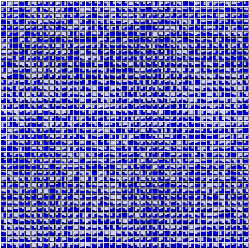
(a) $T=0$, $\alpha=2$

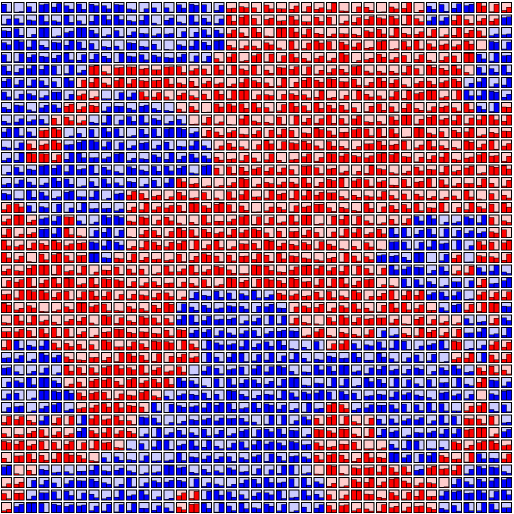
(b) $T=0$, $\alpha=3$

(c) $T=0$, $\alpha=6$

(d) $T=1$, $\alpha=2$

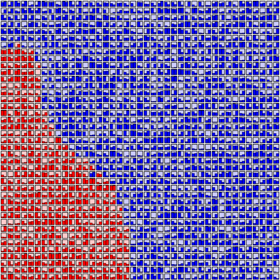
(e) $T=1$, $\alpha=3$

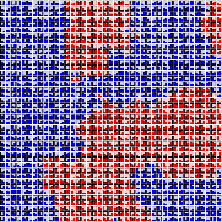
(f) $T=1$, $\alpha=6$

(g) $T=3$, $\alpha=2$

(h) $T=3$, $\alpha=3$

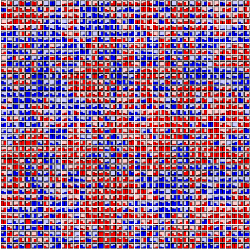
(i) $T=3$, $\alpha=6$

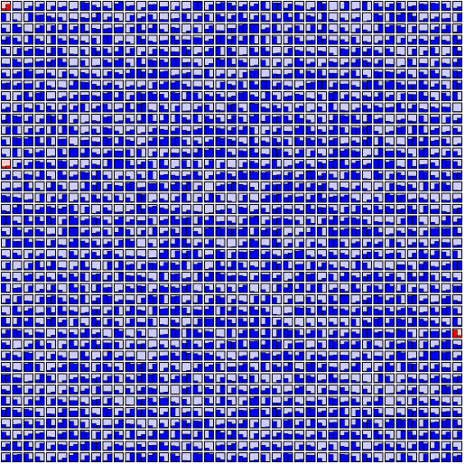
(j) $T=5$, $\alpha=2$

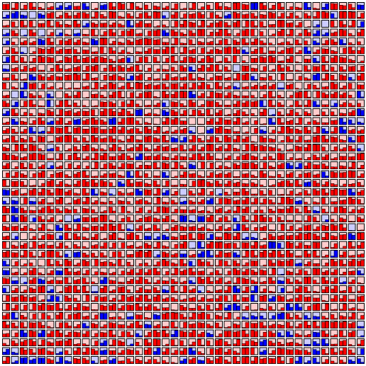
(k) $T=5$, $\alpha=3$

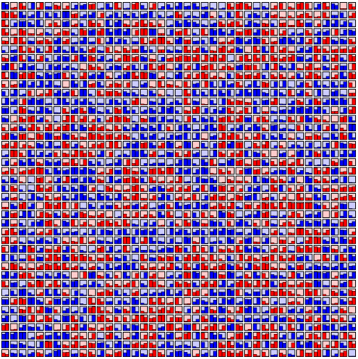
(l) $T=5$, $\alpha=6$

Figure 1: Spatial distribution of opinions $\xi$ for various values of social temperature $T$ and exponent $\alpha$ after $t_{\max}=10^{3}$ time steps. $L^{2}=1681$, $K=2$. Pictures are produced with application Bańcerowski (2017b).

In Fig. 1 the simulation results for $K=2$, $\alpha=$2, 3, 6 and $T=0$, 1, 3, 5 are presented.

Both, $\alpha$ (information flow) and $T$ (noise) influence opinion formation and the spatial distribution of opinions. For $\alpha=2$ the consensus takes place (all actors adopt one of two opinions, except of few actors for large $T$ values). Interesting phenomena for $\alpha=3$ are observed, where the frozen initial system goes into a polarized phase of two large clusters for $T=1$ and into a consensus phase for $T=3$ (one cluster with single actors with a different opinion) before disordering for $T=5$. For $\alpha=6$ many clusters are visible, although the introduction of noise ($T=1$) results in a more ordered system than for other $T$ values. To sum up, the increase of $\alpha$ and $T$ generally causes greater disorder in the system (many clusters with both opinions), but for some values of these parameters their increase leads to order (consensus)—see Fig. 1(h).

In general, we can observe four main types of structures in the formation of opinions for $K=2$:

• formation of single cluster, when all agents adopt one opinion and consensus takes place (Figs. 1(a), 1(d), 1(g), 1(j)),

• the majority of agents with the same opinion and single agents with opposing opinions scattered across the lattice (Fig. 1(h)),

• formation of several large clusters of agents with different opinions—polarisation of the group opinion (Fig. 1(e)),

• formation of plenty small clusters with both opinions (e.g. Figs. 1(b), 1(f)).

III.1.2 $K=3$

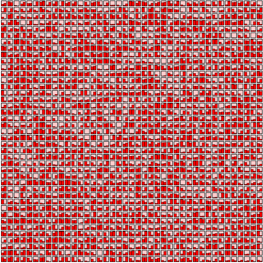
(a) $T=0$, $\alpha=2$

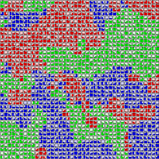
(b) $T=0$, $\alpha=3$

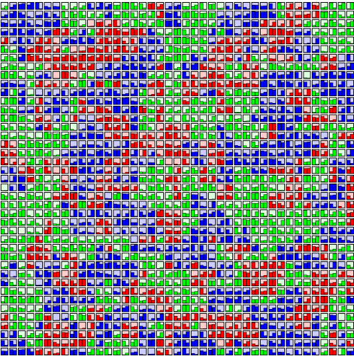
(c) $T=0$, $\alpha=6$

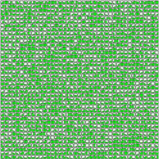
(d) $T=1$, $\alpha=2$

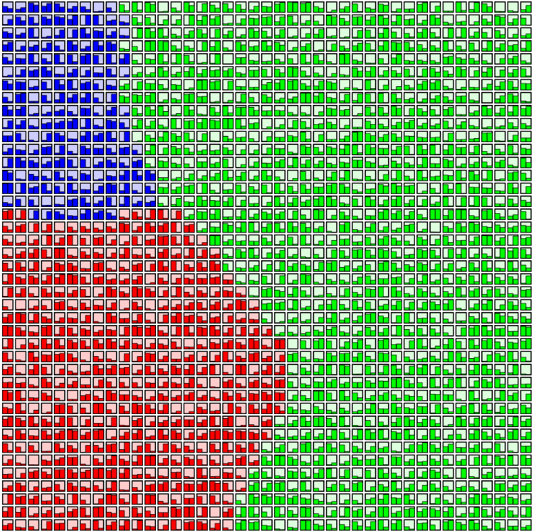
(e) $T=1$, $\alpha=3$

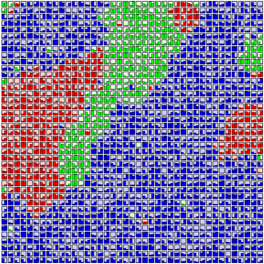
(f) $T=1$, $\alpha=6$

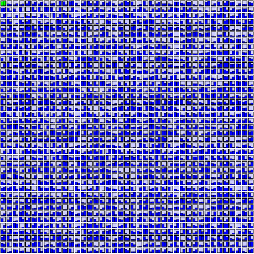
(g) $T=3$, $\alpha=2$

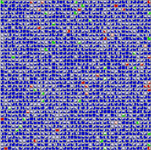
(h) $T=3$, $\alpha=3$

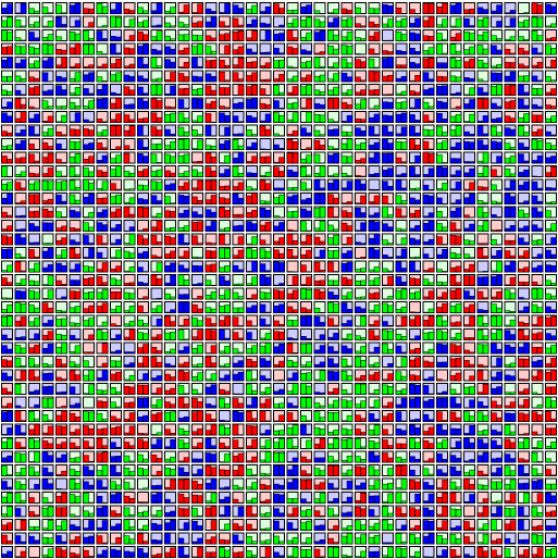
(i) $T=3$, $\alpha=6$

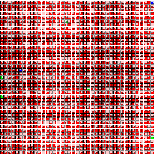
(j) $T=5$, $\alpha=2$

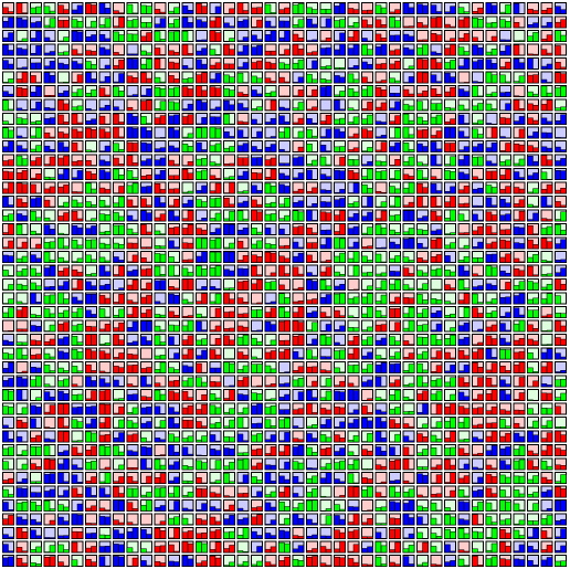
(k) $T=5$, $\alpha=3$

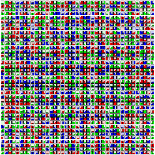
(l) $T=5$, $\alpha=6$

Figure 2: Spatial distribution of opinions $\xi$ for various values of social temperature $T$ and exponent $\alpha$ after $t_{\max}=10^{3}$ time steps. $L^{2}=1681$, $K=3$. Pictures are produced with application Bańcerowski (2017b).

The simulation results for three opinions among actors (where $K=3$, $\alpha=$2, 3, 6 and $T=0$, 1, 3, 5) are presented in Fig. 2.

Similarly to $K=2$, the formation of opinions (the formation of clusters of opinion) depends on the level of noise and the effective range of interactions among actros . For $\alpha=2$, one cluster is formed—consensus take place. For $K=3$ the consensus among actors with three different opinions is also possible for $\alpha=3$. In other cases, many clusters with three opinions or disordered system state are visible.

In general, we can observe four types of structures in the formation of opinions for $K=3$, after thousand time steps:

• formation of single cluster, when all agents adopt one opinion and consensus takes place (Fig. 2(a), 2(d), 2(g), 2(j)),

• the majority of agents with the same opinion and single agents with opposing opinions scattered across the lattice (Fig. 2(h)),

• formation of clusters with all possible opinions—polarisation of the group opinion (Fig. 2(e)),

• formation of plenty small clusters with all opinions (e.g. Fig. 2(b), 2(c), 2(f)).

III.2 Clustering of opinions

In Figs. 1  and 2—discussed in the previous section—different phases of the system depending on the parameters $\alpha$ and $T$ were presented. In order to get a better look at influence of $T$ and $\alpha$ on system behaviour, we anlyzed the histograms $H(\mathcal{S})$ of cluster sizes $\mathcal{S}$ after thousand steps of simulation gathered from hundred simulations (see Figs. 3, 4).

We apply the Hoshen–Kopelman algorithm Hoshen and Kopelman (1976) for clusters detection. In Hoshen–Kopelman algorithm each actor is labelled in such way, that actors with the same opinions and in the same cluster have identical labels. The algorithm allows for cluster detection in multi-dimensional space and for complex neighbourhoods Kotwica et al. (2019); Malarz (2015); Kurzawski and Malarz (2012); Majewski and Malarz (2007); Malarz and Galam (2005), here however, we assume the simplest case, i.e. square lattice with von Neumann neighbourhood (see Fig. 5).

To better explain the phenomena observed in Figs. 3 and 4, the following parameters describing the number and size of clusters were selected:

• average largest cluster size $\langle\mathcal{S}_{\max}\rangle$,

• average cluster number $\langle n_{c}\rangle$,

• average number of small clusters $\langle n_{s}\rangle$.

The example of clusters

• size distribution counting (for preparation histograms $H(\mathcal{S})$ for Figs. 3 and 4),

• average largest value $\langle\mathcal{S}_{\max}\rangle$ (for Figs. 6(a), 7(a)),

• and average numbers $\langle n_{c}\rangle$ (for Figs. 6(b), 7(b)) and $\langle n_{s}\rangle$ (for Figs. 6(c), 7(c))

are provided in Appendix B.

On the left panels of Fig. 6 (for $K=2$) and Fig. 7 (for $K=3$) the ‘heat maps’ and numerical values of $\langle\mathcal{S}_{\max}\rangle$, $\langle n_{c}\rangle$ and $\langle n_{s}\rangle$ for different values of $\alpha$ and $T$ are presented. The supplementary ‘contour maps’, presenting the same data but allowing for better visualisation of non-monotous character of these data, are included on the right panels of these figures. On left panels average values of the larges cluster sizes $\langle\mathcal{S}_{\max}\rangle$ are expressed as a fraction of the number of sites ($L^{2}$). The results were averaged over hundred simulations and gathered after $t_{\max}=1000$ time steps.

As can be seen in Figs. 3, 4, the shapes of histograms are very similar to each other for $K=2$ (Fig. 3) and $K=3$ (Fig. 4). In both cases, there are clear differences in the shape of histograms due to values of $\alpha$ (information flow, effective range of interaction among actors):

• For $\alpha=1$ and $\alpha=2$—where the effective range of interaction is the largest—the unaminity of opinions is achieved (in the case of $\alpha=2$, single agents and rarely small clusters with opposite opinions may appear).

• The most interesting are the histograms for $\alpha=3$ (see figures forming columns from 3(c) to 3(w) and from 4(c) to 4(w)), because the difference in the shape of histograms due to noise ($T$) is also visible. For $\alpha=3$, various phases in the system behaviour are observed. The system from the disordered state, with the growth of $T$ is increasingly ordered. As $T$ increases, more and more clusters appear close to the maximum cluster size in this lattice and more and more small clusters consisting of single agents.

• For $\alpha=6$, histograms have similar shapes for all $T$ values and they indicate the phase of system disorder (a large number of clusters), apart from slight orderliness for $T=1$ (see Figs. 3(h) and 4(h)).

In Figs. 3 and 4, we can also notice that for $\alpha>2$, the greater the randomness in adopting opinions by agents (greater $T$), the more single clusters containing one agent and several agents appear.

(a) $\alpha=1$, $T=0$

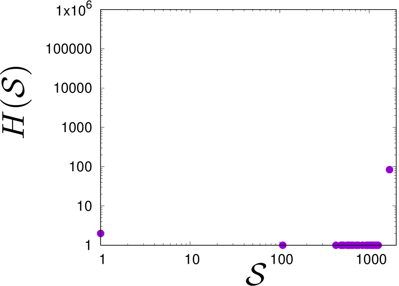
(b) $\alpha=2$, $T=0$

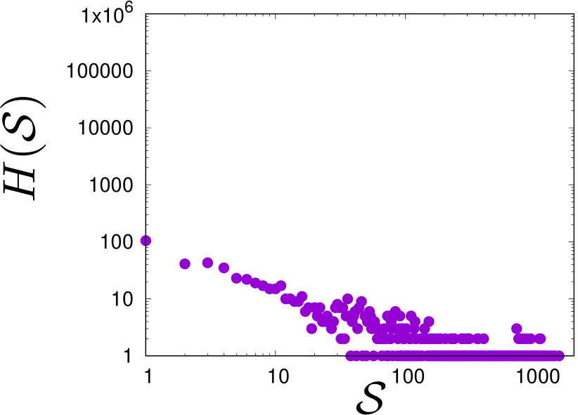
(c) $\alpha=3$, $T=0$

(d) $\alpha=6$, $T=0$

(e) $\alpha=1$, $T=1$

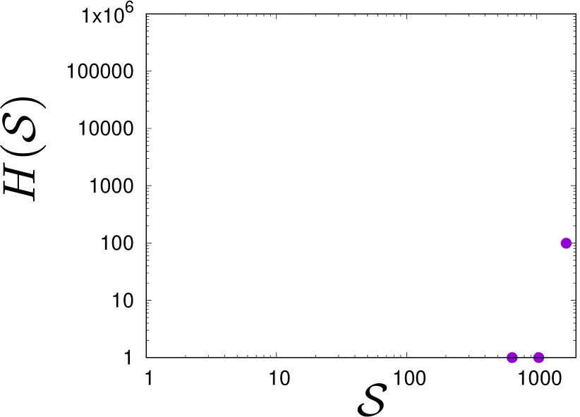
(f) $\alpha=2$, $T=1$

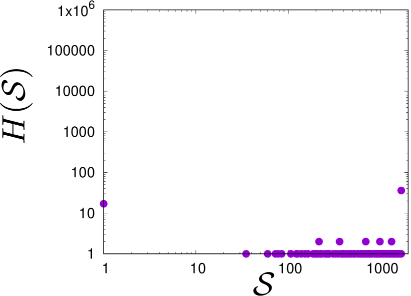
(g) $\alpha=3$, $T=1$

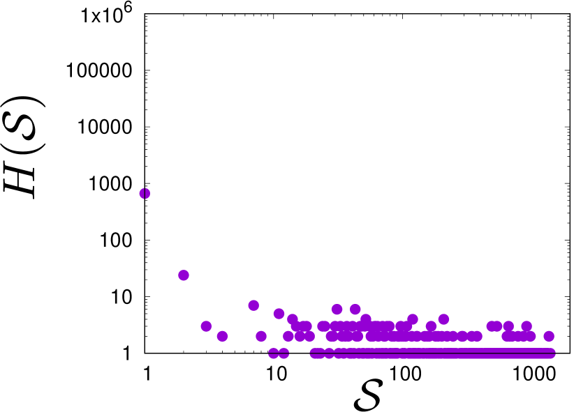
(h) $\alpha=6$, $T=1$

(i) $\alpha=1$, $T=2$

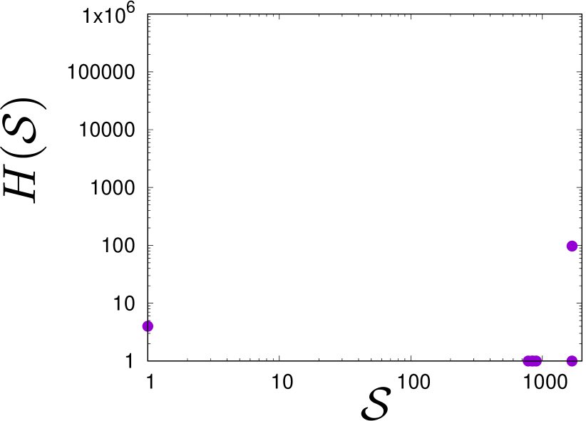
(j) $\alpha=2$, $T=2$

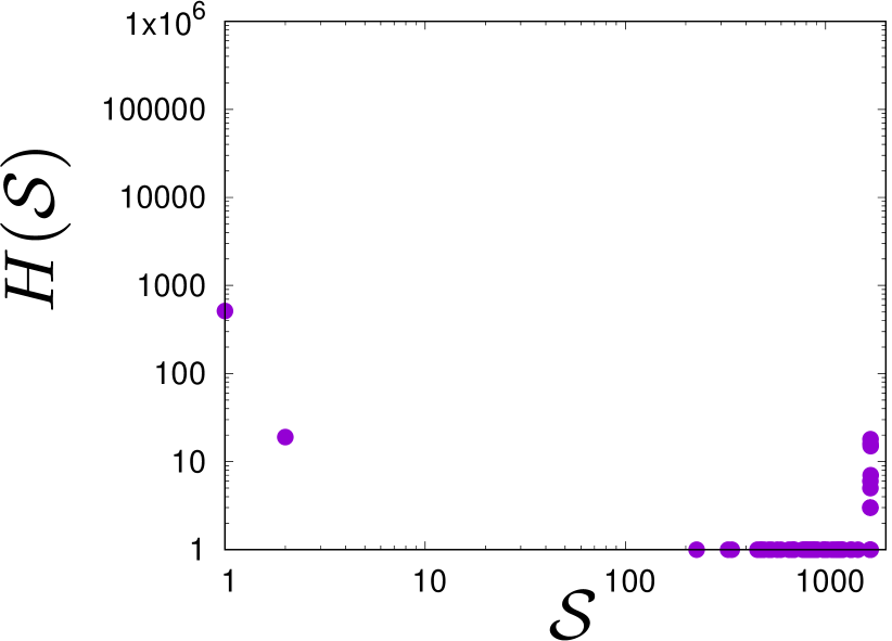
(k) $\alpha=3$, $T=2$

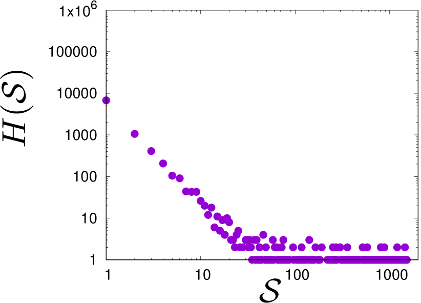
(l) $\alpha=6$, $T=2$

(m) $\alpha=1$, $T=3$

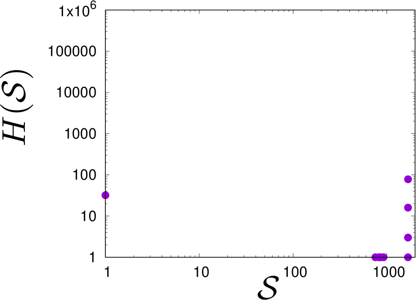
(n) $\alpha=2$, $T=3$

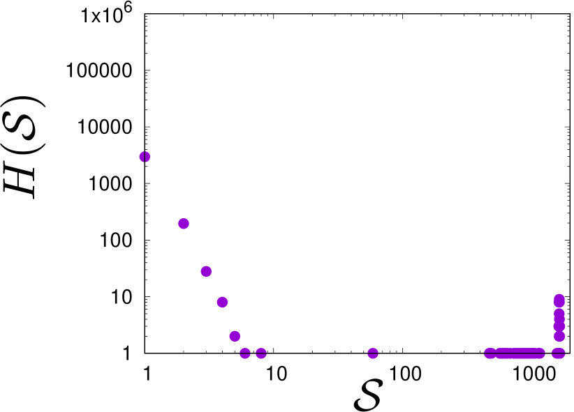
(o) $\alpha=3$, $T=3$

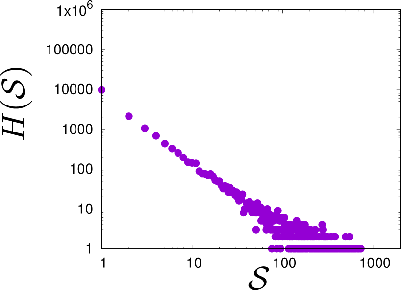
(p) $\alpha=6$, $T=3$

(q) $\alpha=1$, $T=4$

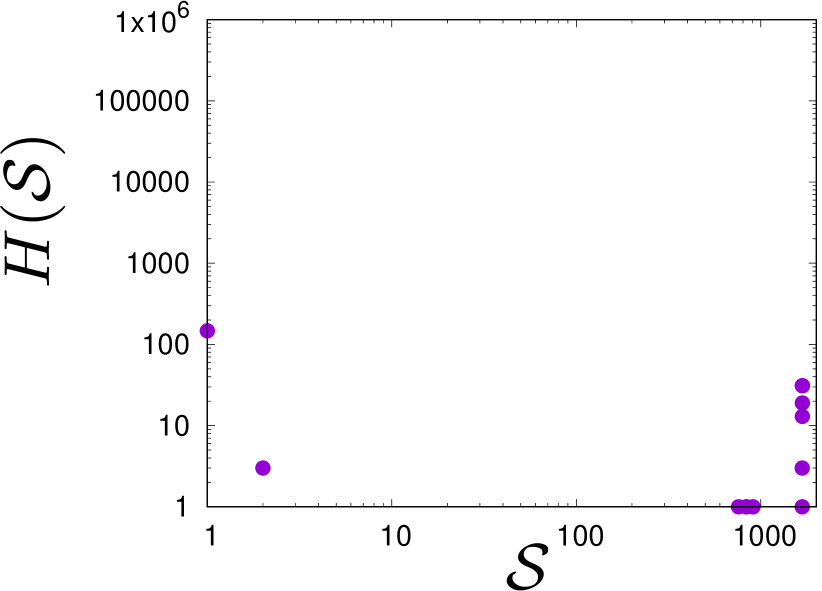
(r) $\alpha=2$, $T=4$

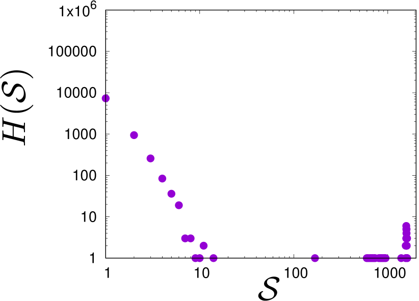
(s) $\alpha=3$, $T=4$

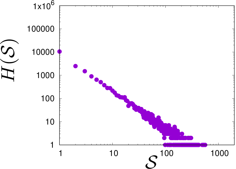
(t) $\alpha=6$, $T=4$

(u) $\alpha=1$, $T=5$

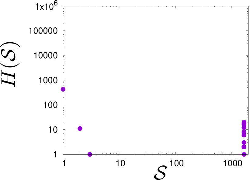
(v) $\alpha=2$, $T=5$

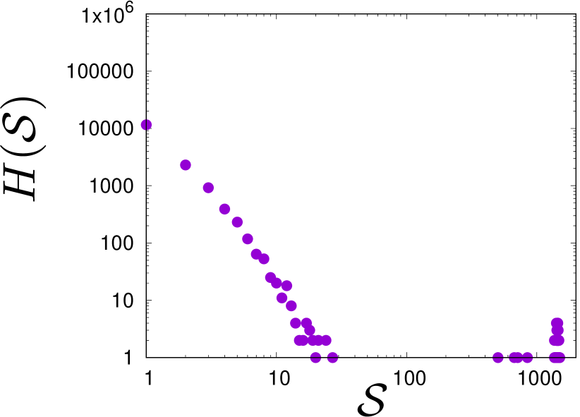
(w) $\alpha=3$, $T=5$

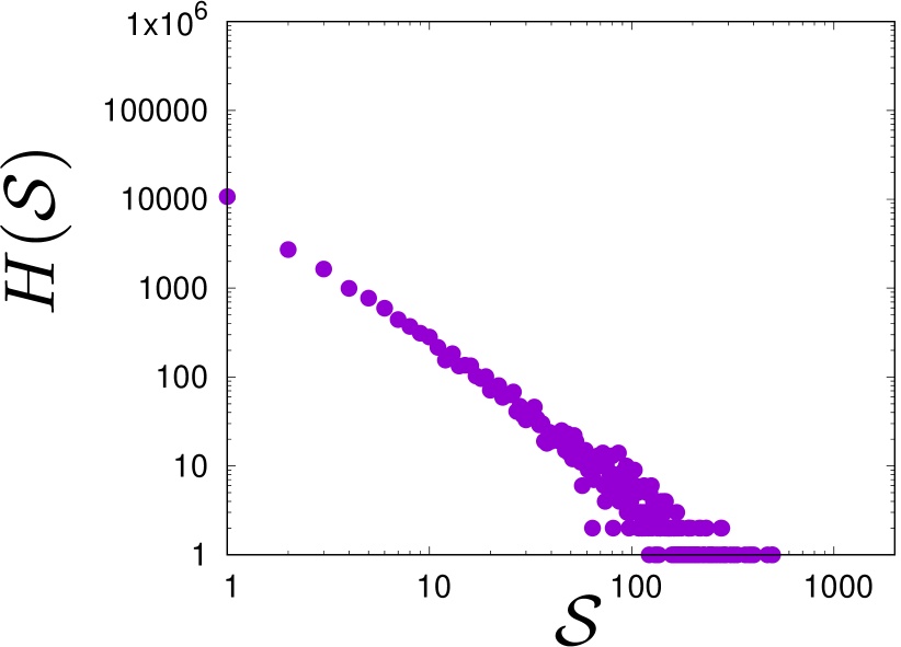
(x) $\alpha=6$, $T=5$

Figure 3: Histograms $H(\mathcal{S})$ of cluster sizes $\mathcal{S}$ for various values of social temperature $T$ and exponent $\alpha$. $L=41$, $K=2$. The results are gathered from hundred runings with different initial conditions after $t_{\max}=1000$ time steps.

(a) $\alpha=1$, $T=0$

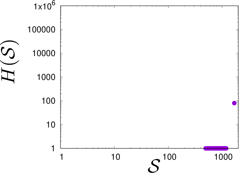
(b) $\alpha=2$, $T=0$

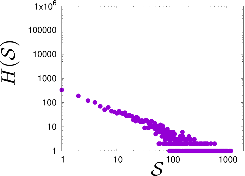
(c) $\alpha=3$, $T=0$

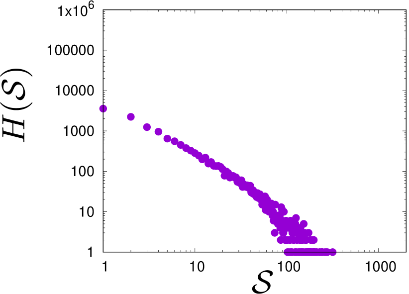
(d) $\alpha=6$, $T=0$

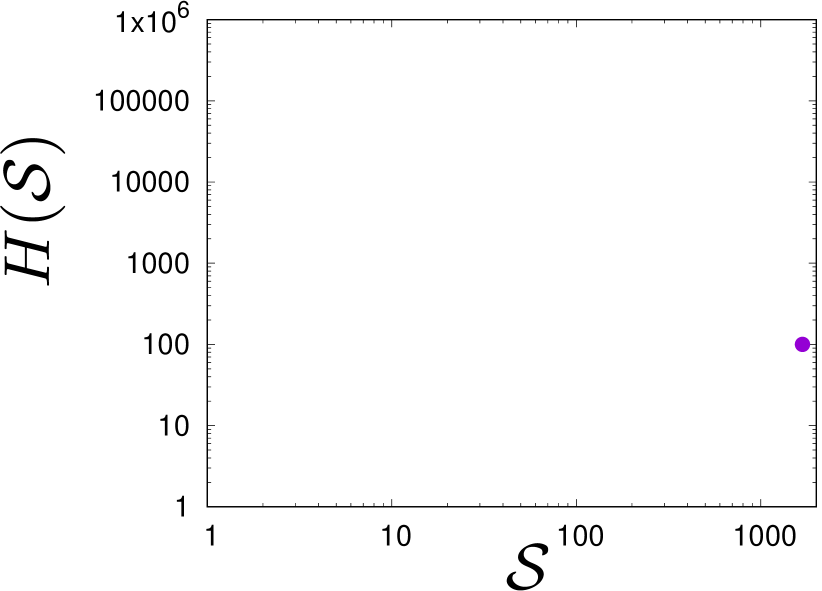
(e) $\alpha=1$, $T=1$

(f) $\alpha=2$, $T=1$

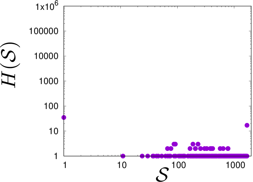
(g) $\alpha=3$, $T=1$

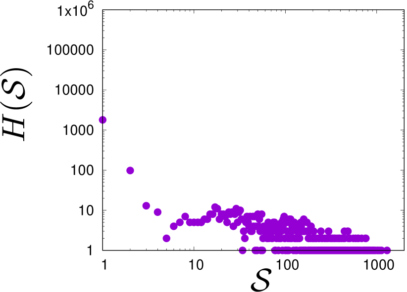
(h) $\alpha=6$, $T=1$

(i) $\alpha=1$, $T=2$

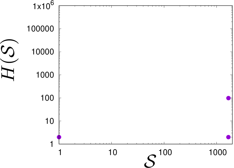
(j) $\alpha=2$, $T=2$

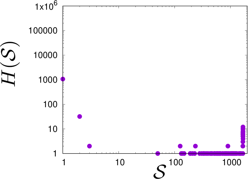
(k) $\alpha=3$, $T=2$

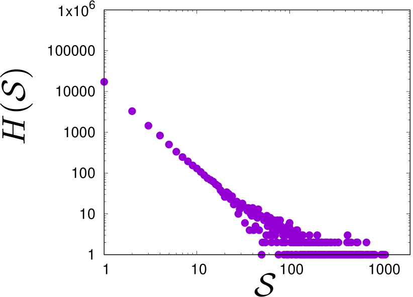
(l) $\alpha=6$, $T=2$

(m) $\alpha=1$, $T=3$

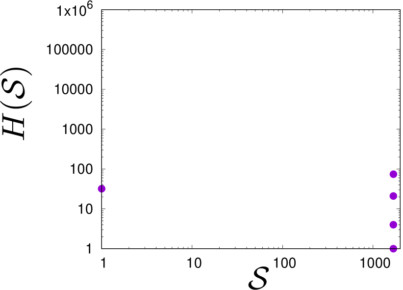
(n) $\alpha=2$, $T=3$

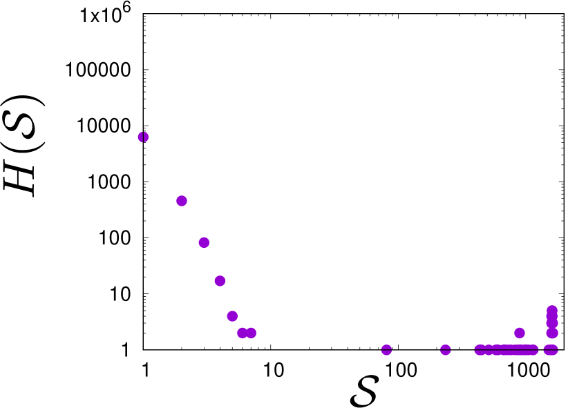
(o) $\alpha=3$, $T=3$

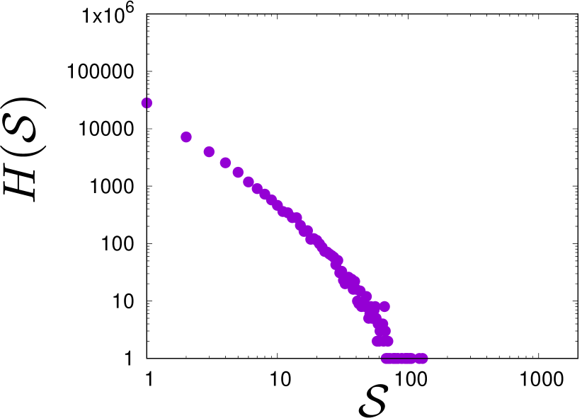
(p) $\alpha=6$, $T=3$

(q) $\alpha=1$, $T=4$

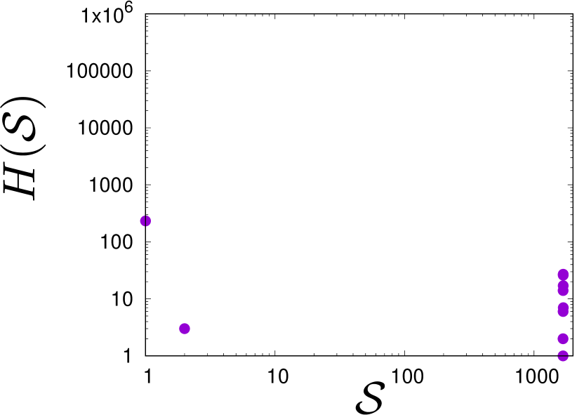
(r) $\alpha=2$, $T=4$

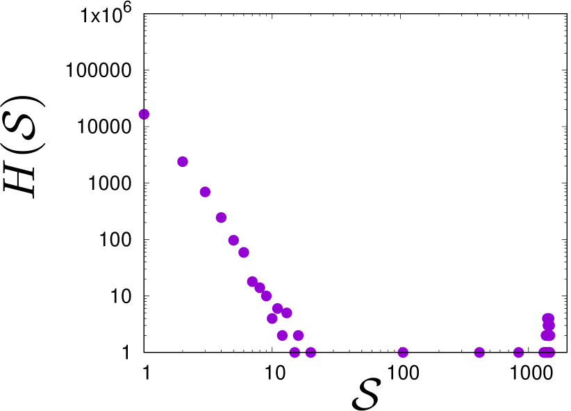
(s) $\alpha=3$, $T=4$

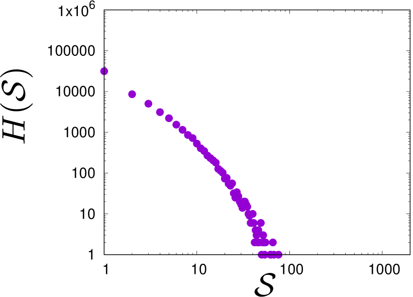
(t) $\alpha=6$, $T=4$

(u) $\alpha=1$, $T=5$

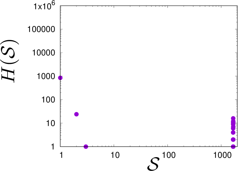
(v) $\alpha=2$, $T=5$

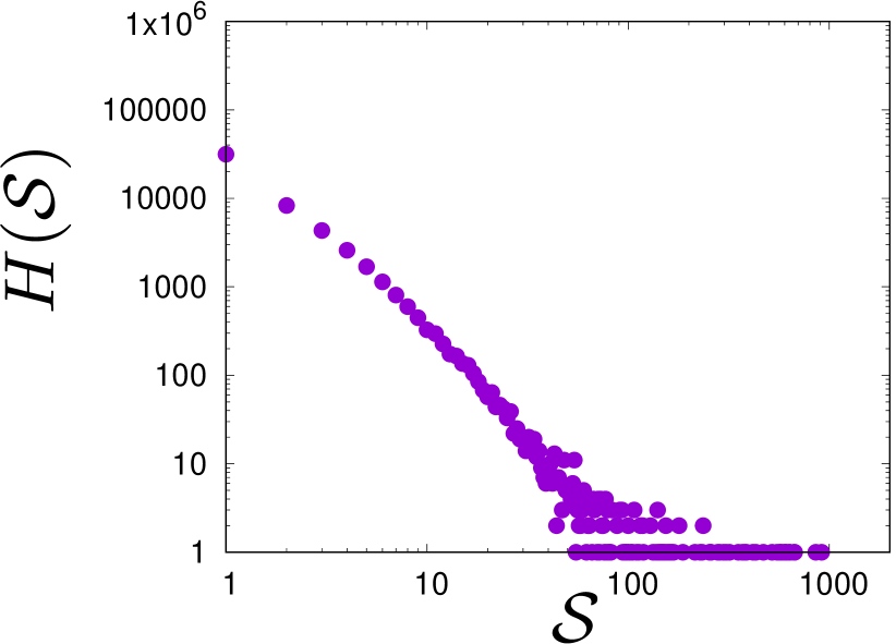
(w) $\alpha=3$, $T=5$

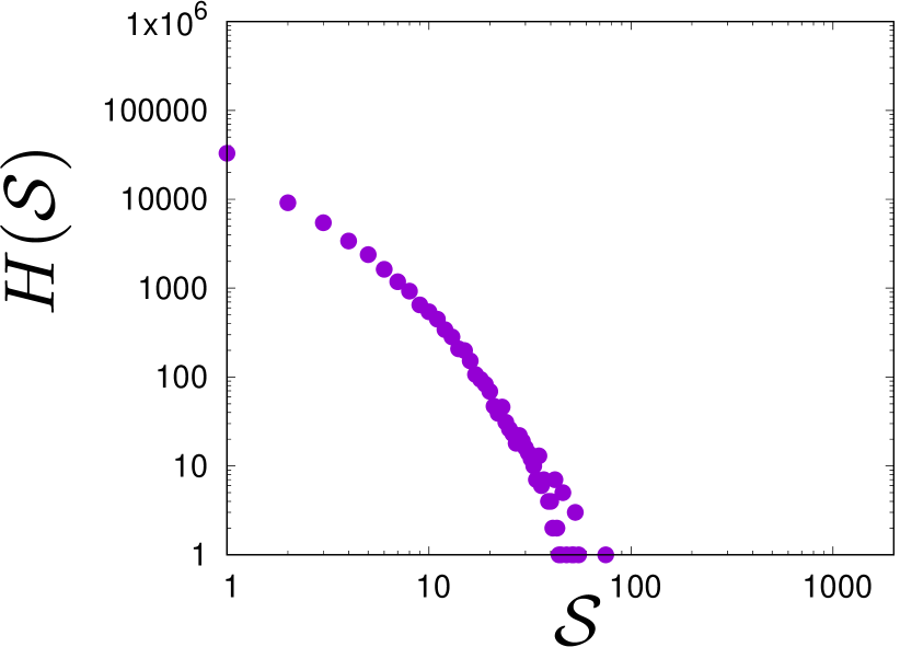
(x) $\alpha=6$, $T=5$

Figure 4: Histogram $H(\mathcal{S})$ of cluster sizes $\mathcal{S}$ for various values of social temperature $T$ and exponent $\alpha$. $L=41$, $K=3$. The results are gathered from hundred runings with different initial conditions after $t_{\max}=1000$ time steps.

Figure 5: The actors with identical opinions $\Xi_{k}$ belong to the common cluster if they are in von Neumann neighbourhood.

III.2.1 $K=2$

As can be seen in Fig. 6(a), the average size of the maximum cluster $\langle\mathcal{S}_{\max}\rangle$ decreases with $\alpha$ for fixed $T$ values. The appearance of noise in the system ($T=1$) slightly organizes the system in relation to the noiseless situation with $T=0$ (see Fig. 6(a)). Indeed, like in earlier studies Ren et al. (2007); Shirado and Christakis (2017), small level of noise brought more order to the system. In addition, the introduction of noise ($T$) in the adoption of opinions causes an increase in $\langle\mathcal{S}_{\max}\rangle$, and then its decrease, which is especially visible for $\alpha>2$. The presense of noise $T>0$ results in greater orderliness of the system but only up to certain $T$ values. Particularly interesting are the large values of $\langle\mathcal{S}_{\max}\rangle$ for $\alpha=3$ and $T=2$, 3, 4. This issue will be disscused below.

Figure 6(b) shows the simulation results of the average number of clusters $\langle n_{c}\rangle$. As can be seen, for fixed noise level $T$, the average number of clusters $\langle n_{c}\rangle$ increases with $\alpha$. This figure also shows that for $\alpha\geq 3$ the average number of clusters increases with $T$. In addition, comparing the results for all $\alpha$ values and for the noiseless system ($T=0$) with the results for small noise level ($T=1$), it can be seen that the introduction of noise results in system ordering.

The average number of small clusters $\langle n_{s}\rangle$ increases with $\alpha$ for fixed values of $T$ (see Fig. 6(c)). For $\alpha=1$ there are no small clusters, and for $\alpha=2$ there are few of them. The increase in the number of small clusters due to $T$ and $\alpha$ is well visible for $\alpha\geq 2$, i.e. when the range of interaction between agents is small.

Considering all results presented in Fig. 6 we can notice, that:

• For $\alpha\leq 2$ we observe the system phase in which there is a consensus (one large cluster representing actors sharing one of the available opinions). The average size of the largest cluster is equal to the size of the lattice. For $\alpha=2$ and $T>2$, the average number of clusters is larger than one, but these higher $\langle n_{c}\rangle$ values only mean the appearance of clusters consisting of single agents, as $|\langle n_{c}\rangle-\langle n_{s}\rangle|\approx 1$, which is shown in Figs. 6(b) and 6(c) and also visible in Figs. 3(n), 3(r), and 3(v).

• An interesting phenomenon can be observed for $\alpha=3$, where the frozen noisless system goes into a more ordered phase for $T=1$ and $T=2$, and into a consensus phase for $T=3$ before disordering at $T=5$ (see. Fig. 6). Polarization of opinion is observed for $T=1$ (about 60% of simulations end with polarization and about 40% of them end with consensus). The average size of the largest cluster contains 83.1% of all agents on the lattice. The average number of clusters is very small and it equals 1.9, and the average number of small clusters is 0.17, which means that the simulations mostly end in a state containing two clusters, one of which is definitely larger than the other. This is also visible in Figs. 1 and 3(g). For $T=2$, more and more system ordering is observed (more and more simulations end with unanimity).

  The second phase in the case of $\alpha=3$ takes place for $T=3$. Despite the high values of noise $T$, the size of the maximum cluster $\langle\mathcal{S}_{\max}\rangle$ is still very large and contains about 90% of all actors (Fig. 6(a)), and the average number of clusters is definitely larger than for $T\leq 2$ (see Fig. 6(b)). An increase in noise level surprisingly causes a kind of order. In this case, one of the opinions dominates, but representatives of the opposite opinion appear in the form of small individual clusters. The average number of small clusters $\langle n_{s}\rangle$ is 32 for $T=3$. This number when compared to the average number of clusters $\langle n_{c}\rangle$ in Fig. 6(b) (33.2 for $T=3$) indicates the emergence of one large cluster and individual small clusters (the average number of small clusters $\langle n_{s}\rangle$ differs by approximately one from the average number of clusters $\langle n_{c}\rangle$). This means, that system evolution toward unaminity of opinion dominates system dynamics for $T=3$.

• For $T=4$, the size of the largest cluster $\langle\mathcal{S}_{\max}\rangle$ is still very large (and reaches ca. 90% of all actors), but although $\langle n_{c}\rangle$ differs from $\langle n_{s}\rangle$ by about one, both the number of clusters and the number of small clusters are definitely larger than in the case of $T=3$ (Fig. 6). So, for $T=4$, the system goes into a disordered phase.

  In the case of $T=5$, the system enters a phase of disorder, because there are definitely more clusters with opposite opinions and they have a larger size than for $T=3$ and $T=4$, which is also visible in Fig. 3(w) and Fig. 1.

  For $\alpha=4$ and $\alpha=5$, when the noise level goes to $T=2$, a slight increase of noise induces more order (see Figs. 6 and 3). This can be seen in the average size of the largest cluster ($\langle\mathcal{S}_{\max}\rangle$ for $T=2$ is larger than for $T=1$) and by comparing the average number of clusters $\langle n_{c}\rangle$ with the average number of small clusters $\langle n_{s}\rangle$ (the difference is smaller than for $T=1$)—Fig. 6.

  When the interaction effectively takes place only among the nearest neighbors (for $\alpha=6$), this effect vanishes.

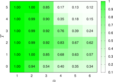
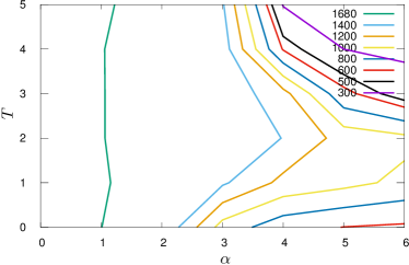
(a) Average largest cluster size $\langle\mathcal{S}_{\max}\rangle$ (in left panel normalized to $L^{2}$).

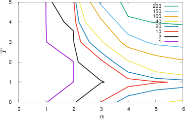
(b) Average number of clusters $\langle n_{c}\rangle$.

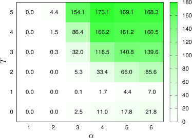
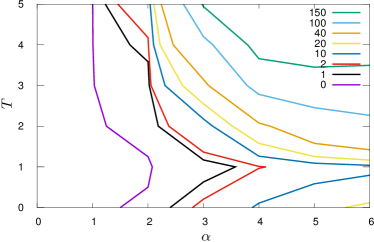
(c) Average number of small cluster $\langle n_{s}\rangle$.

Figure 6: Average (a) largest cluster size $\langle\mathcal{S}_{\max}\rangle$, (b) number of clusters $\langle n_{c}\rangle$ and (c) average number of small clusters $\langle n_{s}\rangle$ for various values of noise level $T$ and exponent $\alpha$. $L^{2}=1681$, $K=2$. The results are averaged over hundred runings with different initial conditions and measured after $t_{\max}=10^{3}$ time steps.

To check the system behaviour for $K=2$, simulations for $L=21$ and $L=61$ were also carried out. The simulations for the smaller and larger network of agents showed results consistent with the presented for networks with size $L=41$. Slight differences were observed for $\alpha=3$, where for $T=1$ and $T=2$ after 1000 steps of simulation, in the case of a smaller network, consensus is more often observed, and for a larger network less often.

To sum up, three main types of structures in the formation of opinions for $K=2$ are observed:

• formation of single cluster, when all agents adopt one opinion and consensus takes place (for $\alpha\leq 2$, $T=1$, 2, 3, 4, 5 and $\alpha=3$, $T=2$, 3, 4),

• greater orderliness—polarization of opinions in clusters ($\alpha=3$, $T=1$, $T=2$ and for $\alpha=3$, 4, and $T=2$),

• formation of plenty small clusters with both opinions—disorder (for other values of $\alpha$ and $T$).

III.2.2 $K=3$

In Fig. 7 the simulation results for $K=3$ are presented. The average size of the largest cluster $\langle\mathcal{S}_{\max}\rangle$ (Fig. 7(a)) decreases with $\alpha$ for fixed values of the noise level $T$, as it was observed for $K=2$. For $\alpha=1$ and $\alpha=2$, $\langle\mathcal{S}_{\max}\rangle$ is equal to the number of all actors on the lattice. For $\alpha>2$, the average size of the largest cluster $\langle\mathcal{S}_{\max}\rangle$ increases up to a certain value of $T$, and then decreases. This inflection point is nearly $T=2$.

In the case of the average number of clusters $\langle n_{c}\rangle$—which is presented in Fig. 7(b)—this number is the smallest for $T=1$, i.e. as soon as noise is introduced to the system. Similarly to the case of $K=2$, for fixed noise level $T$, the average number of clusters $\langle n_{c}\rangle$ increases with $\alpha$. Fig. 7(b) also shows, that for $\alpha>2$ the average number of clusters $\langle n_{c}\rangle$ increases with $T$ for all $T>1$.

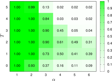
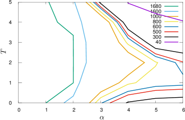
(a) Average largest cluster size $\langle\mathcal{S}_{\max}\rangle$ (in left panel normalized to $L^{2}$).

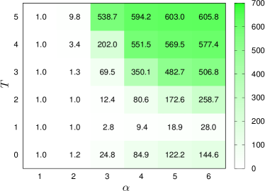
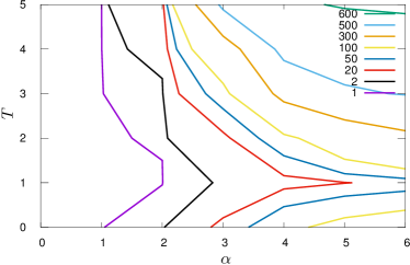
(b) Average number of clusters $\langle n_{c}\rangle$.

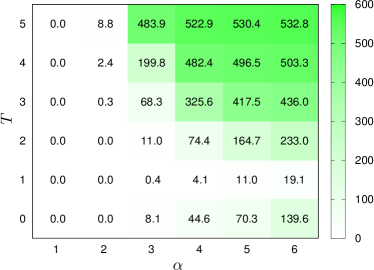
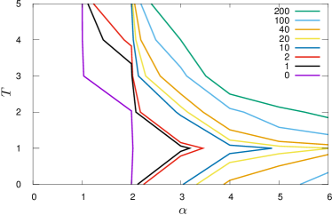
(c) Average number of small cluster $\langle n_{s}\rangle$.

Figure 7: Average (a) largest cluster size $\langle\mathcal{S}_{\max}\rangle$, (b) number of clusters $\langle n_{c}\rangle$ and (c) average number of small clusters $\langle n_{s}\rangle$ for various values of noise level $T$ and exponent $\alpha$. $L^{2}=1681$, $K=3$. The results are averaged over hundred runings with different initial conditions and measured after $t_{\max}=10^{3}$ time steps.

The average number of small clusters $\langle n_{s}\rangle$, similarly to the case of $K=2$, increases with the increase $T$ and $\alpha$ (Fig. 7(c)). For $\alpha=1$ there are no small clusters, and for $\alpha=2$ they appear only for $T>3$. The increase in the number of small clusters $\langle n_{s}\rangle$ with increase of $T$ and $\alpha$ is clearly visible for $\alpha>2$.

As the simulation results suggest—also in the case of $K=3$ opinions available in the system—various phases in the system behaviour can be observed. These phases are induced by interplay of noise level $T$ and effective range of interaction among actors $\alpha$. First of all, for $\alpha=1$ and all $T$ values, a large cluster with one opinion is formed (consensus takes place). In this case, $\langle\mathcal{S}_{\max}\rangle$ are equal to the number of all agents on the lattice, and the average number of clusters $\langle n_{c}\rangle$ is one (see Figs. 7(a), 7(b)—left panels). Single cluster is also created in the case of $\alpha=2$. As can be seen in Figs. 7(a) and 7(b) the average largest cluster size is close to the system size $\langle\mathcal{S}_{\max}\rangle\approx L^{2}$, and the average number of clusters is close to one $\langle n_{c}\rangle\approx 1$. The exceptions occur for large values of the noise level $T\geq 4$, but this is associated with the appearance of single small and short-living clusters, which is typical for high randomness in actors behaviour. In this situation the average number of small clusters differs by approximately one from the average number of clusters $|\langle n_{c}\rangle-\langle n_{s}\rangle|\leq 1$. These results are confirmed by the data in Figs. 7(b) and 7(c).

As in the case of two opinions ($K=2$), interesting phenomena are visible for $\alpha=3$. For $T=1$, polarization of opinions is observed. In 80% of cases of the final system state two or three clusters of opinions are created, one of which is larger than the others ($\mathcal{S}_{\max}/L^{2}=0.73$, see Fig. 2(e)). For $T=2$, as in the case of two opinions, more ordering is observed than for $T=1$. Consequently, by increasing noise level, for $T=3$ a consensus takes place (one large cluster and small clusters with only single actor). The average size of the largest cluster is still very large and contains about 90% of all actors in the lattice. Although the average number of clusters $\langle n_{c}\rangle$ is quite large, when compared with the average number of small clusters $\langle n_{s}\rangle$ it indicates the existence of one large cluster and single small clusters (the average number of clusters differs by approximately one from the average number of small clusters $|\langle n_{c}\rangle-\langle n_{s}\rangle|\approx 1$—see Figs. 7(b) and 7(c)). For $\alpha=3$ and $T=4$, despite the still high $\langle\mathcal{S}_{\max}\rangle$, the number of small clusters increases, which leads to a disorder phase for $T=5$. The difference between average number of clusters $\langle n_{c}\rangle$ and average number of small clusters $\langle n_{s}\rangle$ is definitely greater than one cluster $|\langle n_{c}\rangle-\langle n_{s}\rangle|\gg 1$ (cf. Figs. 7(a), 7(b)).

For $\alpha>3$ and all $T$ values, system disorder (many clusters of all opinions) is visible—Figs. 2 and 4, with the exception of $\alpha=4$ and $\alpha=5$, when a slight increase of noise ($T=2$) does induce more order than for $T=1$ (see Figs. 7 and 4). As for $K=2$, in the case of three opinions, simulations for $L=21$ and $L=61$ were also carried out. The simulations for the smaller and larger network of agents showed similar results to the presented for networks with size $L=41$. Slight differences were observed for $\alpha=3$, and $T=1$ and $T=2$ after 1000 steps of simulation, where ordering in clusters is more visible in small networks than in large ones.

To sum up, we can notice three main phases in the behaviour of the model for $K=3$:

• formation of single cluster, when all agents adopt one opinion and consensus takes place (for $\alpha\leq 2$; $T=1$, 2, 3, 4, 5 and $\alpha=3$, $T=3$),

• greater orderliness—polarization of opinions in clusters (sometimes one cluster or ordering opinions in two or three clusters, where two or three opinions occur ($\alpha=3$, $T=1$, $T=2$ and for $\alpha=3$, 4, $T=2$),

• formation of plenty clusters with all three opinions—disorder (for other values of $\alpha$ and $T$).

IV Summary and conclusions

In this paper, we are interested in how opinions are formed and how they spread in the community. We were investigating how flow of information in the community and randomness of human behaviour influence formation of opinions, its spreading and its polarisation. The community was presented as a square lattice of linear size $L$ with open boundary conditions, which is fully filled by actors.

The flow of information was controled by the parameter $\alpha$. This parameter reflects the effective impact of the neighbourhood on the opinion of the actors. In case of low values of this parameter, actors shape their opinion basing on a large number of actors (including distant neighbours). In our research, we also take into account the randomness in adopting opinions, which is expressed in the noise parameter $T$. The larger $T$, the more often actors adopt opinions which have no greatest impact on them

Each actor in our model is characterised, in addition to the opinion, by two parameters. They are the intensity of persuasion ($p_{i}$) and the intensity of support ($s_{i}$). The higher the value of persuasiveness $p_{i}$, the actor more easier convincing other actors to accept his/her opinion. With bigger ($s_{i}$), the agent convinces more strongly other actors. These parameters therefore determine the effectiveness of which an individual may interact with or influence other individuals by changing or confirming their opinions. In all performed simulations, we adopted random values of ($p_{i}$) and ($s_{i}$) parameters, which brings us closer to the social reality, in which we do not usually have data on the strength with which the unit affects other units. Simulations have been carried out when actors have a choice of two or three opinions on a given topic. First, the spatial distribution of opinions after thousand steps of simulation was analysed. The simulations showed how clusters of opinion are formed depending on (i) the flow of information in the agents’ network, and (ii) the randomness in forming the opinion. For both $K=2$ and $K=3$ we can see consensus, polarization of opinions and the formation of many clusters of available opinions.

As it was shown in previous sections, the clustering of opinions is influenced by both the level of randomness in actors’ decisions (noise) and the impact coming from neighbours. Generally, the size of the largest cluster of opinions decreases with the increase of $\alpha$ (as can be seen by inspection of columns in Figs. 1 and 2). Furthermore, the number of clusters for both $K=2$ and $K=3$ increases with $\alpha$, i.e. the smaller effective range of actors’ interaction the more difficult forming clusters of opinions. Intuitively, an increase in the number of clusters with an increase in noise level $T$ is expected. In fact, the number of clusters is growing, but for $\alpha=3$ and $T=3$ we have one cluster and single agents with opposite opinions, as can be seen in Figs. 1 and 2. In this case, introducing of noise ($T$) leads to consensus with single representatives of the opposite opinion(s). In addition, for $\alpha\geq 3$, a slight increase of noisa elevel ($T=2$) induces more order than for $T=1$ (with the exception for $\alpha=6$ when the interaction effectively takes place only among the nearest neighbors).

In summary, the simulations showed that opinion formation and spread is influenced by both: efficiency of information flow among actors and noise level. Better information flow, i.e. better contacts among actors facilitates the spread of opinion and its formation. In the case of small values of $\alpha$ (when information flow is very good) the unaminity of opinion is reached and consensus takes place, as in most sociophysical models of opinion dynamics Castellano et al. (2009), for both, two and three opinions available in the system. For large values of $\alpha$—when effectively only the nearest neighbours excert impact on given actor—the polarisation of opinions is weak and there are many small groups of actors with the same opinion.

The lack of consensus in models is mainly caused by the introduction of noise Carro et al. (2016) or anti-conformism Galam (2004). In the presented model there is no global agreement also for $T=0$ (when there is no noise). For $T=0$ and $\alpha\geq 3$ clusters of both opinions (or three for $K=3$) appear. In addition, in the presented model, noise for certain values of $\alpha$ promotes unanimity. This situation occurs for $\alpha=3$ (both for $K=2$ and $K=3$), when the system from the frozen state, with increasing noise $T$, achieves the consensus state for $T=3$, before disordering for $T=5$.

As it was mentioned earlier, many studies indicate irrationality and unpredictability in the process of forming opinions Kowalska-Pyzalska et al. (2014, 2014); Byrka et al. (2016); Stadelmann and Torgler (2013); Sobkowicz (2018). As our simulations have shown, this randomness in adopting opinions (noise) plays a crucial role. A low level of noise (low $T$ values) results in less clusters of opinion than in the absence of noise ($T=0$). However, the most interesting is the fact, that the high noise levels ($T=2$, 3, 4) results in a more ordered system than for small values of noise $T$ (this is the case with $\alpha=3$). Thus, noise favours consensus and polarization of opinion in groups, but only when the influence of distant neighbours is significant. If the exchange of opinions takes place only with the nearest neighbors, this effect is not observed.

In future research, we intend to take into account the impact of strong leaders on the opinion dynamics. Also the influence of external sources of information (for instance the impact of mass media) is worth of investigation.

Appendix A Example of small system evolution ($L=3$, $K=3$)

To better explain the model rules we calculate social impact on single actor for case of small lattice ($L=3$). We assume $K=3$ opinions available in the system marked as ‘red’ ($\Xi_{1}$), ‘blue’ ($\Xi_{2}$) and ‘green’ ($\Xi_{3}$). We will calculate the impact exerting by nine actors on the actors labelled as ‘5’ and ‘9’ in Fig. 8. We assume the supportiveness $s_{i}=i/10$ and persuasiveness $p_{i}=1-i/10$.

According to Eq. (2) to evaluate the opinion $\xi_{5}(t+1)$ in the next time step we have to calculated $K=3$ impacts exerted on actor $i=5$ for three opinions available in the system.

As $\xi_{5}(t)=\Xi_{2}$ (‘blue’) we use Eq. (2a) to calculate impact

$$I_{5,\text{blue}}(t)=4\mathcal{J}_{s}\left(\dfrac{q(s_{5})}{g(d_{5,5})}+\dfrac{q(s_{6})}{g(d_{5,6})}+\dfrac{q(s_{9})}{g(d_{5,9})}\right),$$ (5)

from all actors with ‘blue’ opinions (i.e. for $i=6,9$), including actor $i=5$ himself/herself. The impacts from actors with ‘red’ and ‘green’ opinions are calculated basing on Eq. (2b):

$$I_{5,\text{red}}(t)=4\mathcal{J}_{p}\left(\dfrac{q(p_{1})}{g(d_{5,1})}+\dfrac{q(p_{3})}{g(d_{5,3})}+\dfrac{q(p_{4})}{g(d_{5,4})}+\dfrac{q(p_{7})}{g(d_{5,7})}\right),$$ (6)

$$I_{5,\text{green}}(t)=4\mathcal{J}_{p}\left(\dfrac{q(p_{2})}{g(d_{5,2})}+\dfrac{q(p_{8})}{g(d_{5,8})}\right),$$ (7)

Figure 8: (Colour online) Example of small lattice with nine actors and three opinions. The numbers are actors labels $i$. The colours correspond to various actors opinions (‘red’—$\Xi_{1}$, ‘blue’—$\Xi_{2}$ and ‘green’—$\Xi_{3}$).

We assume identity function for scaling functions $\mathcal{J}_{S}(x)\equiv x$, $\mathcal{J}_{P}(x)\equiv x$, $q(x)\equiv x$ and the distance scaling function $g(x)=1+x^{\alpha}$, with $\alpha=2$. These assumptions yield

$$I_{5,\text{blue}}(t)=4\left(\dfrac{s_{5}}{1+d_{5,5}^{2}}+\dfrac{s_{6}}{1+d_{5,6}^{2}}+\dfrac{s_{9}}{1+d_{5,9}^{2}}\right)=4\left(\dfrac{0.5}{1+0^{2}}+\dfrac{0.6}{1+1^{2}}+\dfrac{0.9}{1+\sqrt{2}^{2}}\right)=4.4,$$ (8)

$$I_{5,\text{red}}(t)=4\left(\dfrac{p_{1}}{1+d_{5,1}^{2}}+\dfrac{p_{3}}{1+d_{5,3}^{2}}+\dfrac{p_{4}}{1+d_{5,4}^{2}}+\dfrac{p_{7}}{1+d_{5,7}^{2}}\right)\\ =4\left(\dfrac{0.9}{1+\sqrt{2}^{2}}+\dfrac{0.7}{1+\sqrt{2}^{2}}+\dfrac{0.6}{1+1^{2}}+\dfrac{0.3}{1+\sqrt{2}^{2}}\right)=7.(3),$$ (9)

$$I_{5,\text{green}}(t)=4\left(\dfrac{p_{2}}{1+d_{5,2}^{2}}+\dfrac{p_{8}}{1+d_{5,8}^{2}}\right)\\ =4\left(\dfrac{0.8}{1+1^{2}}+\dfrac{0.2}{1+1^{2}}\right)=2.$$ (10)

For $T=0$ the largest impact on actor $i=5$ is excreted by ‘red’ actors and thus—according to Eq. (1)—actor $i=5$ in the next time step will change his/her opinion from ‘blue’ ($\xi_{5}(t)=\Xi_{2}$) to ‘red’ ($\xi_{5}(t+1)=\Xi_{1}$).

For $T>0$ we calculate probabilities $P_{5,\text{blue}}$, $P_{5,\text{red}}$ and $P_{5,\text{green}}$ of choosing opinion by actor $i=5$ (see Eqs. (4a)–(4b)). For example, for $T=1$ these probabilities are

$$\begin{split}P_{5,\text{blue}}&=\dfrac{\exp(I_{5,\text{blue}}/1)}{P_{1}},\\ P_{5,\text{red}}&=\dfrac{\exp(I_{5,\text{red}}/1)}{P_{1}},\\ P_{5,\text{green}}&=\dfrac{\exp(I_{5,\text{green}}/1)}{P_{1}},\end{split}$$ (11)

while for $T=10$ we have

$$\begin{split}P_{5,\text{blue}}&=\dfrac{\exp(I_{5,\text{blue}}/10)}{P_{10}},\\ P_{5,\text{red}}&=\dfrac{\exp(I_{5,\text{red}}/10)}{P_{10}},\\ P_{5,\text{green}}&=\dfrac{\exp(I_{5,\text{green}}/10)}{P_{10}},\end{split}$$ (12)

where normalisation constants are

$$P_{1}=\exp(I_{5,\text{blue}}/1)+\exp(I_{5,\text{red}}/1)+\exp(I_{5,\text{green}}/1)$$

and

$$P_{10}=\exp(I_{5,\text{blue}}/10)+\exp(I_{5,\text{red}}/10)+\exp(I_{5,\text{green}}/10).$$

The calculated probabilities for $T=1$ are

$$\begin{split}P_{5,\text{blue}}&=\dfrac{\exp(4.4/1)}{e^{4.4}+e^{7.(3)}+e^{2}}\approx 0.050,\\ P_{5,\text{red}}&=\dfrac{\exp(7.(3)/1)}{e^{4.4}+e^{7.(3)}+e^{2}}\approx 0.945,\\ P_{5,\text{green}}&=\dfrac{\exp(2/1)}{e^{4.4}+e^{7.(3)}+e^{2}}\approx 0.005,\end{split}$$ (13)

while for $T=10$ we have

$$\begin{split}P_{5,\text{blue}}&=\dfrac{\exp(4.4/10)}{e^{0.44}+e^{0.7(3)}+e^{0.2}}\approx 0.320,\\ P_{5,\text{red}}&=\dfrac{\exp(7.(3)/10)}{e^{0.44}+e^{0.7(3)}+e^{0.2}}\approx 0.429,\\ P_{5,\text{green}}&=\dfrac{\exp(2/10)}{e^{0.44}+e^{0.7(3)}+e^{0.2}}\approx 0.251.\end{split}$$ (14)

For non-deterministic version of algorithm (i.e. for $T>0$) still the most probably state $\xi_{5}(t+1)$ is $\Xi_{1}$ (‘red’). But probability of such evolution for actor $i=5$ decreases from 100% for $T=0$ to 94.5% for $T=1$ and to 42.9% for $T=10$ to become 33.3%$=1/K$ for $T\to\infty$.

Let us repeat these calculation for actor $i=9$:

$$I_{9,\text{blue}}(t)=4\mathcal{J}_{s}\left(\dfrac{q(s_{5})}{g(d_{9,5})}+\dfrac{q(s_{6})}{g(d_{9,6})}+\dfrac{q(s_{9})}{g(d_{9,9})}\right),$$ (15)

$$I_{9,\text{red}}(t)=4\mathcal{J}_{p}\left(\dfrac{q(p_{1})}{g(d_{9,1})}+\dfrac{q(p_{3})}{g(d_{9,3})}+\dfrac{q(p_{4})}{g(d_{9,4})}+\dfrac{q(p_{7})}{g(d_{9,7})}\right),$$ (16)

$$I_{9,\text{green}}(t)=4\mathcal{J}_{p}\left(\dfrac{q(p_{2})}{g(d_{9,2})}+\dfrac{q(p_{8})}{g(d_{9,8})}\right),$$ (17)

$$I_{9,\text{blue}}(t)=4\left(\dfrac{s_{5}}{1+d_{9,5}^{2}}+\dfrac{s_{6}}{1+d_{9,6}^{2}}+\dfrac{s_{9}}{1+d_{9,9}^{2}}\right)=4\left(\dfrac{0.5}{1+\sqrt{2}^{2}}+\dfrac{0.6}{1+1^{2}}+\dfrac{0.9}{1+0^{2}}\right)=5.4(6),$$ (18)

$$I_{9,\text{red}}(t)=4\left(\dfrac{p_{1}}{1+d_{9,1}^{2}}+\dfrac{p_{3}}{1+d_{9,3}^{2}}+\dfrac{p_{4}}{1+d_{9,4}^{2}}+\dfrac{p_{7}}{1+d_{9,7}^{2}}\right)\\ =4\left(\dfrac{0.9}{1+(2\sqrt{2})^{2}}+\dfrac{0.7}{1+2^{2}}+\dfrac{0.6}{1+\sqrt{5}^{2}}+\dfrac{0.3}{1+2^{2}}\right)=1.6,$$ (19)

$$I_{9,\text{green}}(t)=4\left(\dfrac{p_{2}}{1+d_{9,2}^{2}}+\dfrac{p_{8}}{1+d_{9,8}^{2}}\right)\\ =4\left(\dfrac{0.8}{1+\sqrt{5}^{2}}+\dfrac{0.2}{1+1^{2}}\right)=0.9(3).$$ (20)

For $T=0$ the largest impact on actor $i=9$ is excreted by ‘blue’ actors and thus—according to Eq. (1)—actor $i=9$ in the next time step will sustain his/her ‘blue’ opinion ($\xi_{9}(t+1)=\xi_{9}(t)=\Xi_{2}$). Two factors influence the difference in actors $i=5$ and $i=9$ opinion in time $(t+1)$. Namely, the difference in supportiveness of these two actors and their distance to ‘red’ actors: actor $i=5$ has moderate supportiveness ($s_{5}=0.5$) and his/her distance to ‘red’ actors is no longer than $\sqrt{2}$. In contrast, actor $i=9$ has very high supportiveness ($s_{9}=0.9$) and distance to ‘red’ actors no shorter than 2. Please note however, that ultimate fate of the system is the state with the unanimity of opinions. As we have shown above, in the next time step at least the actor in the middle of the system ($i=5$) will convert his/her opinion to the ‘red’ one. The same presumably will occur for actor $i=2$ who has low supportiveness ($s_{2}=0.2$) and who has only a single supporter. Thus in time $(t+3)$ all actors will convert to the supporters of the ‘red’ opinion.

For $T>0$ we calculate probabilities $P_{9,\text{blue}}$, $P_{9,\text{red}}$ and $P_{9,\text{green}}$ of choosing opinion by actor $i=9$ (see Eqs. (4a)–(4b)). For example, for $T=1$ these probabilities are

$$\begin{split}P_{9,\text{blue}}&=\dfrac{\exp(I_{9,\text{blue}}/1)}{P_{1}},\\ P_{9,\text{red}}&=\dfrac{\exp(I_{9,\text{red}}/1)}{P_{1}},\\ P_{9,\text{green}}&=\dfrac{\exp(I_{9,\text{green}}/1)}{P_{1}},\end{split}$$ (21)

while for $T=10$ we have

$$\begin{split}P_{9,\text{blue}}&=\dfrac{\exp(I_{9,\text{blue}}/10)}{P_{10}},\\ P_{9,\text{red}}&=\dfrac{\exp(I_{9,\text{red}}/10)}{P_{10}},\\ P_{9,\text{green}}&=\dfrac{\exp(I_{9,\text{green}}/10)}{P_{10}},\end{split}$$ (22)

where normalisation constants are

$$P_{1}=\exp(I_{9,\text{blue}}/1)+\exp(I_{9,\text{red}}/1)+\exp(I_{9,\text{green}}/1)$$

and

$$P_{10}=\exp(I_{9,\text{blue}}/10)+\exp(I_{9,\text{red}}/10)+\exp(I_{9,\text{green}}/10).$$

The calculated probabilities for $T=1$ are

$$\begin{split}P_{9,\text{blue}}&=\dfrac{\exp(5.4(6)/1)}{e^{5.4(6)}+e^{1.6}+e^{0.9(3)}}\approx 0.969,\\ P_{9,\text{red}}&=\dfrac{\exp(1.6/1)}{e^{5.4(6)}+e^{1.6}+e^{0.9(3)}}\approx 0.020,\\ P_{9,\text{green}}&=\dfrac{\exp(0.9(3)/1)}{e^{5.4(6)}+e^{1.6}+e^{0.9(3)}}\approx 0.011,\end{split}$$ (23)

while for $T=10$ we have

$$\begin{split}P_{9,\text{blue}}&=\dfrac{\exp(5.4(6)/10)}{e^{0.54(6)}+e^{0.16}+e^{0.09(3)}}\approx 0.432,\\ P_{9,\text{red}}&=\dfrac{\exp(1.6/10)}{e^{0.54(6)}+e^{0.16}+e^{0.09(3)}}\approx 0.293,\\ P_{9,\text{green}}&=\dfrac{\exp(0.9(3)/10)}{e^{0.54(6)}+e^{0.16}+e^{0.09(3)}}\approx 0.275.\end{split}$$ (24)

Similarly to the actor $i=5$, the increase of the social temperature reduces chance of keeping initial opinion for actor $i=9$. For $T=10$ these probabilities do not differ from $1/K$ for more than 0.1.

Appendix B Small example of clustering ($L=10$, $K=3$)

Two sites are in the same cluster if they are adjacent (in von Neumann neighbourhood, Fig. 5) to each other and simultaneously actors at these sites share the same opinion. The Hoshen–Kopelman algorithm allows for sites labelling in such way that sites in the same cluster have the same labels and sites in different cluster have different labels. Examples of sites labelling for $L=10$ and $K=3$ are presented in Figs. 9(a) and 9(b), where $n_{c}=11$ and $n_{c}=4$ clusters have been identified, respectively. The average number of cluster for these two lattice realization is $\langle n_{c}\rangle=(11+4)/2=7.5$. The number of sites in each cluster defines its size $\mathcal{S}$. For these two lattice ralizations the largest culsters are labelled as 1 and 5 (Fig. 9(a)) and as 14 (Fig. 9(b)) and their sizes are $\mathcal{S}_{\max}=25$ and $\mathcal{S}_{\max}=54$, respectively. Thus average largest cluster size is $\langle\mathcal{S}_{\max}\rangle=(25+54)/2=39.5$. In given example histogram $H(\mathcal{S})$ of clusters sizes is presented in Table 1. Basing on Table 1 we evaluate number of small clusters (with $\mathcal{S}\leq 5$) as 4+1+2+1=8. As this sum comes from merging results of two lattice realization the average number of small clusters is $\langle n_{s}\rangle=8/2=4$.

(a)

(b)

Figure 9: Example of sites labelling for $K=3$ and $L=10$ and two lattice realizations.

Table 1: Histogram of cluster sizes $\mathcal{S}$ for lattices presented in Fig. 9.

labels $i$:	6, 9, 11, 15	3	8, 12	10	2	4, 7	1, 5	13	14
$\mathcal{S}$:	1	2	3	5	8	14	25	42	54
$n(\mathcal{S})$:	4	1	2	1	1	2	2	1	1

Appendix C Source codes

In Listings 1 and 2 the Fortran 95 codes allowing for reproductions of data for Figs. 3, 4, 6, 7 (for both, noiseless and non-deterministic version of simulations) are presented.

The module settings provides model parameters including lattice size $L$ (Xmax and Ymax), number of opinions $K$ (Kmax), number of time steps $t_{\max}$ (Tmax) and number of lattice realizations (Run) .

In module utils the scaling functions $g(x)$ and $q(x)$ as well as the Euclidean distance $d(x,y)$ are defined. Also the reclassify function for Hoshen–Kopelman algorithm is defined there.

The main program starts in line 52. The actors supportiveness ($s_{i}$) and persuasiveness ($p_{i}$) are initialised randomly in lines 85–90, while initial actors opinions ($\xi_{i}$) are given in lines 93–98. Loop 88 provides time evolution of the system. Loop 77 realises Hoshen–Kopelman algorithm of sites (actors) labelling for $t=0$. In loop 99 the system characteristics after the system time evolution is completed are calculated. Loop 777 realises averaging procedure over independent runnnigs for various initial conditions.

C.1 $T=0$

An input data ($\alpha$ parameter) is read in line 71. In lines 272–275 histograms $H(\mathcal{S})$ of clusters sizes $\mathcal{S}$ are printed. In line 278 values of $\langle n_{c}\rangle$, $\langle S\rangle$ (not presented in this paper) and $\langle\mathcal{S}_{\max}\rangle$ are printed.

Listing 1: Fortan95 code implementing Eq. (1) i.e. for $T=0$

⬇

1!!! Latane-Nowak-Szamrej model + Hoshen-Kopelman algorithm

2!!! K. Malarz

3!!! created: Tue, 21 May 2019, 13:06:13 CEST

4!!! revised: Sun, 05 Apr 2020, 14:43:19 CEST

5

6!!! ================================================================

7module settings

8!!! ================================================================

9implicit none

10

11integer, parameter :: Xmax=41,Ymax=41,Tmax=1000,Kmax=2,L2=(Xmax+1)*(Ymax+1),Run=100

12real*8, parameter :: T=0.d0

13real*8 :: alpha

14end module settings

15

16!!! ================================================================

17module utils

18!!! ================================================================

19use settings

20implicit none

21contains

22

23real*8 function g(x)

24 real*8 :: x

25 g=1.0d0+x**alpha

26end function

27

28real*8 function q(x)

29 real*8 :: x

30 q=x

31end function

32

33real*8 function d(x1,y1,x2,y2)

34 integer :: x1,y1,x2,y2

35 d=dsqrt((1.d0*x1-1.d0*x2)**2 + (1.d0*y1-1.d0*y2)**2)

36end function

37

38integer function reclassify(ix)

39integer :: ix

40integer, dimension (0:Xmax,0:Ymax) :: label

41integer, dimension (L2) :: iclass

42common/block/ label, iclass

43

44reclassify=iclass(ix)

4590 if(iclass(reclassify).eq.reclassify) return

46reclassify=iclass(reclassify)

47goto 90

48end function

49

50end module utils

51

52!!! ################################################################

53program Latane_Hoshen_Kopelman

54!!! ################################################################

55use settings

56use utils

57implicit none

58integer :: x,y,it, xx,yy,k,kk,strongest_k,irun,maxlabel,Smax,largestS

59real :: r

60real*8 :: sump,strongest_I,avenc,aveS,aveSmax

61

62integer, dimension (0:Xmax,0:Ymax) :: label

63integer, dimension (L2) :: iclass

64integer, dimension (0:Xmax,0:Ymax) :: xi

65integer, dimension (0:Xmax*Ymax) :: isize, histograminrun,histogram

66integer, dimension (0:Xmax*Ymax,Kmax) :: histogramK

67real*8, dimension (Xmax,Ymax) :: p, s

68real*8, dimension (Xmax,Ymax,Kmax) :: I, prob

69common/block/ label, iclass

70

71 read *,alpha

72 print ’(A3,7A11)’,’###’,’Xmax’,’Ymax’,’K’,’alpha’,’T’,’tmax’,’run’

73 print ’(A3,3I11,2F11.3,2I11)’,’###’,Xmax,Ymax,Kmax,alpha,T,Tmax,Run

74

75 histogram=0

76 aveSmax=0.d0

77 aveS=0.d0

78 avenc=0.d0

79

80 do 777 irun=1,Run

81 histograminrun=0

82! print *,’#########’

83! print *,’# irun=’,irun

84

85 do x=1,Xmax !! initial state

86 do y=1,Ymax

87 s(x,y)=rand()

88 p(x,y)=rand()

89 enddo

90 enddo

91

92 it=0

93 xi=0

94 do x=1,Xmax

95 do y=1,Ymax

96 xi(x,y)=1+Kmax*rand()

97 enddo

98 enddo

99

100 histogramK=0

101

102 do 77 k=1,Kmax

103 isize=0

104

105 label=L2

106 do kk=1,L2

107 iclass(kk)=kk

108 enddo

109 maxlabel=0

110

111 do x=1,Xmax

112 do y=1,Ymax

113 if(xi(x,y).eq.k) then !! labeling clusters

114 if(xi(x-1,y).eq.k .or. xi(x,y-1).eq.k) then

115 !! reclassifing neighbouring sites

116 if(xi(x-1,y).eq.k) label(x-1,y)=reclassify(label(x-1,y))

117 if(xi(x,y-1).eq.k) label(x,y-1)=reclassify(label(x,y-1))

118 label(x,y)=min(label(x-1,y),label(x,y-1))

119 iclass(label(x-1,y))=label(x,y)

120 iclass(label(x,y-1))=label(x,y)

121 else

122 maxlabel=maxlabel+1

123 label(x,y)=maxlabel

124 endif

125 endif

126 enddo

127 enddo

128 ! reclassifing all occupied sites

129 do x=1,Xmax

130 do y=1,Ymax

131 if((xi(x,y).eq.k) .and. (label(x,y).gt.iclass(label(x,y)))) label(x,y)=reclassify(label(x,y))

132 enddo

133 enddo

134

135 do x=1,Xmax

136 do y=1,Ymax

137 if(xi(x,y).eq.k) isize(label(x,y))=isize(label(x,y))+1

138 enddo

139 enddo

140

141 do kk=1,Xmax*Ymax

142 histogramK(isize(kk),k)=histogramK(isize(kk),k)+1

143 enddo

144

14577 enddo

146

147 do 88 it=1,Tmax !!! time evolution

148 I=0.0d0

149 do x=1,Xmax

150 do y=1,Ymax

151 do xx=1,Xmax

152 do yy=1,Ymax

153 if(xi(x,y).eq.xi(xx,yy)) then

154 I(x,y,xi(xx,yy))=I(x,y,xi(xx,yy))+q(s(xx,yy))/g(d(x,y,xx,yy))

155 else

156 I(x,y,xi(xx,yy))=I(x,y,xi(xx,yy))+q(p(xx,yy))/g(d(x,y,xx,yy))

157 endif

158 enddo

159 enddo

160 enddo

161 enddo

162

163 do x=1,Xmax

164 do y=1,Ymax

165 do k=1,Kmax

166 I(x,y,k)=4.0d0*I(x,y,k)

167 enddo

168 enddo

169 enddo

170

171 do x=1,Xmax

172 do y=1,Ymax

173 strongest_I=I(x,y,1)

174 strongest_k=1

175 do k=2,Kmax

176 if(I(x,y,k).gt.strongest_I) then

177 strongest_I=I(x,y,k)

178 strongest_k=k

179 endif

180 enddo

181 xi(x,y)=strongest_k

182 enddo

183 enddo

18488 enddo !!! time evolution

185

186! print *,’# it=’,it,’xi:’

187! do x=1,Xmax

188! print ’(41I5)’,(xi(x,y),y=1,Ymax)

189! enddo

190 histogramK=0

191 Smax=0

192

193 do 99 k=1,Kmax

194 isize=0

195

196! print *,"# k=",k

197 label=L2

198 do kk=1,L2

199 iclass(kk)=kk

200 enddo

201 maxlabel=0

202

203 do x=1,Xmax

204 do y=1,Ymax

205 if(xi(x,y).eq.k) then ! labeling clusters

206 if(xi(x-1,y).eq.k .or. xi(x,y-1).eq.k) then

207 ! reclassifing neighbouring sites

208 if(xi(x-1,y).eq.k) label(x-1,y)=reclassify(label(x-1,y))

209 if(xi(x,y-1).eq.k) label(x,y-1)=reclassify(label(x,y-1))

210 label(x,y)=min(label(x-1,y),label(x,y-1))

211 iclass(label(x-1,y))=label(x,y)

212 iclass(label(x,y-1))=label(x,y)

213 else

214 maxlabel=maxlabel+1

215 label(x,y)=maxlabel

216 endif

217 endif

218 enddo

219 enddo

220 ! reclassifing all occupied sites

221 do x=1,Xmax

222 do y=1,Ymax

223 if((xi(x,y).eq.k) .and. (label(x,y).gt.iclass(label(x,y)))) label(x,y)=reclassify(label(x,y))

224 enddo

225 enddo

226

227! do x=1,Xmax

228! print ’(41I5)’,(label(x,y),y=1,Ymax)

229! enddo

230

231 do x=1,Xmax

232 do y=1,Ymax

233 if(xi(x,y).eq.k) isize(label(x,y))=isize(label(x,y))+1

234 enddo

235 enddo

236

237 do kk=1,Xmax*Ymax

238 histogramK(isize(kk),k)=histogramK(isize(kk),k)+1

239 enddo

240

241! print *,"# histogram, irun=",irun," k=",k

242 do kk=1,Xmax*Ymax

243! if(histogramK(kk,k).gt.0) print *,kk,histogramK(kk,k)

244 histograminrun(kk)=histograminrun(kk)+histogramK(kk,k)

245 enddo

246

247 do kk=Xmax*Ymax,1,-1

248 if(histogramK(kk,k).gt.0) then

249 largestS=kk

250 goto 33

251 endif

252 enddo

25333 Smax=max(Smax,largestS)

254! print *,"# largest S=",largestS

255! print *,"# Smax=",Smax

256

25799 enddo

258

259! do k=1,Xmax*Ymax

260! if(histograminrun(k).gt.0) print *,k,histograminrun(k)

261! enddo

262! print *,"# nc=",sum(histograminrun)

263 avenc=avenc+1.d0*sum(histograminrun)

264 aveSmax=aveSmax+1.d0*Smax

265 do k=1,Xmax*Ymax

266 aveS=aveS+(1.d0*k*histograminrun(k))/(1.d0*sum(histograminrun))

267 histogram(k)=histogram(k)+histograminrun(k)

268 enddo

269

270777 enddo

271

272 print *,"# total histogram:"

273 do k=1,Xmax*Ymax

274 if(histogram(k).gt.0) print *,k,histogram(k)

275 enddo

276

277 print ’(A2,A3,5A9)’,"#","K","T","alpha","<nc>","<S>","<Smax>"

278 print ’(A2,I3,5F9.3)’,"#",Kmax,T,alpha,avenc/(1.d0*Run),aveS/(1.d0*Run),aveSmax/(1.d0*Run)

279

280end program Latane_Hoshen_Kopelman

C.2 $T>0$

An input data ($\alpha$ and $T$ parameters) are read in line 71. In lines 284–287 histograms $H(\mathcal{S})$ of clusters size $\mathcal{S}$ are printed. In line 290 values of $\langle n_{c}\rangle$, $\langle S\rangle$ (not presented in this paper), $\langle\mathcal{S}_{\max}\rangle$ are printed.

Listing 2: Fortan95 code implementing Eq. (4) i.e. for $T>0$

⬇

1!!! Latane-Nowak-Szamrej model + Hoshen-Kopelman algorithm

2!!! K. Malarz

3!!! created: Tue, 21 May 2019, 13:06:13 CEST

4!!! revised: Sun, 05 Apr 2020, 14:43:19 CEST

5

6!!! ================================================================

7module settings

8!!! ================================================================

9implicit none

10

11integer, parameter :: Xmax=41,Ymax=41,Tmax=1000,Kmax=2,L2=(Xmax+1)*(Ymax+1),Run=100

12real*8 :: T

13real*8 :: alpha

14end module settings

15

16!!! ================================================================

17module utils

18!!! ================================================================

19use settings

20implicit none

21contains

22

23real*8 function g(x)

24 real*8 :: x

25 g=1.0d0+x**alpha

26end function

27

28real*8 function q(x)

29 real*8 :: x

30 q=x

31end function

32

33real*8 function d(x1,y1,x2,y2)

34 integer :: x1,y1,x2,y2

35 d=dsqrt((1.d0*x1-1.d0*x2)**2 + (1.d0*y1-1.d0*y2)**2)

36end function

37

38integer function reclassify(ix)

39integer :: ix

40integer, dimension (0:Xmax,0:Ymax) :: label

41integer, dimension (L2) :: iclass

42common/block/ label, iclass

43

44reclassify=iclass(ix)

4590 if(iclass(reclassify).eq.reclassify) return

46reclassify=iclass(reclassify)

47goto 90

48end function

49

50end module utils

51

52!!! ################################################################

53program Latane_Hoshen_Kopelman

54!!! ################################################################

55use settings

56use utils

57implicit none

58integer :: x,y,it, xx,yy,k,kk,strongest_k,irun,maxlabel,Smax,largestS

59real :: r

60real*8 :: sump,avenc,aveS,aveSmax

61

62integer, dimension (0:Xmax,0:Ymax) :: label

63integer, dimension (L2) :: iclass

64integer, dimension (0:Xmax,0:Ymax) :: xi

65integer, dimension (0:Xmax*Ymax) :: isize, histograminrun,histogram

66integer, dimension (0:Xmax*Ymax,Kmax) :: histogramK

67real*8, dimension (Xmax,Ymax) :: p, s

68real*8, dimension (Xmax,Ymax,Kmax) :: I, prob

69common/block/ label, iclass

70

71 read *,T,alpha

72 print ’(A3,7A11)’,’###’,’Xmax’,’Ymax’,’K’,’alpha’,’T’,’tmax’,’run’

73 print ’(A3,3I11,2F11.3,2I11)’,’###’,Xmax,Ymax,Kmax,alpha,T,Tmax,Run

74

75 histogram=0

76 aveSmax=0.d0

77 aveS=0.d0

78 avenc=0.d0

79

80 do 777 irun=1,Run

81 histograminrun=0

82! print *,’#########’

83! print *,’# irun=’,irun

84

85 do x=1,Xmax !! initial state

86 do y=1,Ymax

87 s(x,y)=rand()

88 p(x,y)=rand()

89 enddo

90 enddo

91

92 it=0

93 xi=0

94 do x=1,Xmax

95 do y=1,Ymax

96 xi(x,y)=1+Kmax*rand()

97 enddo

98 enddo

99

100 histogramK=0

101

102 do 77 k=1,Kmax

103 isize=0

104

105 label=L2

106 do kk=1,L2

107 iclass(kk)=kk

108 enddo

109 maxlabel=0

110

111 do x=1,Xmax

112 do y=1,Ymax

113 if(xi(x,y).eq.k) then !! labeling clusters

114 if(xi(x-1,y).eq.k .or. xi(x,y-1).eq.k) then

115 !! reclassifing neighbouring sites

116 if(xi(x-1,y).eq.k) label(x-1,y)=reclassify(label(x-1,y))

117 if(xi(x,y-1).eq.k) label(x,y-1)=reclassify(label(x,y-1))

118 label(x,y)=min(label(x-1,y),label(x,y-1))

119 iclass(label(x-1,y))=label(x,y)

120 iclass(label(x,y-1))=label(x,y)

121 else

122 maxlabel=maxlabel+1

123 label(x,y)=maxlabel

124 endif

125 endif

126 enddo

127 enddo

128 ! reclassifing all occupied sites

129 do x=1,Xmax

130 do y=1,Ymax

131 if((xi(x,y).eq.k) .and. (label(x,y).gt.iclass(label(x,y)))) label(x,y)=reclassify(label(x,y))

132 enddo

133 enddo

134

135 do x=1,Xmax

136 do y=1,Ymax

137 if(xi(x,y).eq.k) isize(label(x,y))=isize(label(x,y))+1

138 enddo

139 enddo

140

141 do kk=1,Xmax*Ymax

142 histogramK(isize(kk),k)=histogramK(isize(kk),k)+1

143 enddo

144

14577 enddo

146

147 do 88 it=1,Tmax !!! time evolution

148 I=0.0d0

149 do x=1,Xmax

150 do y=1,Ymax

151 do xx=1,Xmax

152 do yy=1,Ymax

153 if(xi(x,y).eq.xi(xx,yy)) then

154 I(x,y,xi(xx,yy))=I(x,y,xi(xx,yy))+q(s(xx,yy))/g(d(x,y,xx,yy))

155 else

156 I(x,y,xi(xx,yy))=I(x,y,xi(xx,yy))+q(p(xx,yy))/g(d(x,y,xx,yy))

157 endif

158 enddo

159 enddo

160 enddo

161 enddo

162

163 do x=1,Xmax

164 do y=1,Ymax

165 do k=1,Kmax

166 I(x,y,k)=4.0d0*I(x,y,k)

167 enddo

168 enddo

169 enddo

170

171 do x=1,Xmax

172 do y=1,Ymax

173 sump=0.0d0

174 do k=1,Kmax

175 prob(x,y,k)=dexp(I(x,y,k)/T)

176 sump=sump+prob(x,y,k)

177 enddo

178 do k=1,Kmax

179 prob(x,y,k)=prob(x,y,k)/sump

180 enddo

181 enddo

182 enddo

183

184 do x=1,Xmax

185 do y=1,Ymax

186 r=rand()

187 sump=0.0d0

188 do k=1,Kmax

189 sump=sump+prob(x,y,k)

190 if(r.lt.sump) goto 666

191 enddo

192666 xi(x,y)=k

193 enddo

194 enddo

195

19688 enddo !!! time evolution

197

198! print *,’# it=’,it,’xi:’

199! do x=1,Xmax

200! print ’(41I5)’,(xi(x,y),y=1,Ymax)

201! enddo

202 histogramK=0

203 Smax=0

204

205 do 99 k=1,Kmax

206 isize=0

207

208! print *,"# k=",k

209 label=L2

210 do kk=1,L2

211 iclass(kk)=kk

212 enddo

213 maxlabel=0

214

215 do x=1,Xmax

216 do y=1,Ymax

217 if(xi(x,y).eq.k) then ! labeling clusters

218 if(xi(x-1,y).eq.k .or. xi(x,y-1).eq.k) then

219 ! reclassifing neighbouring sites

220 if(xi(x-1,y).eq.k) label(x-1,y)=reclassify(label(x-1,y))

221 if(xi(x,y-1).eq.k) label(x,y-1)=reclassify(label(x,y-1))

222 label(x,y)=min(label(x-1,y),label(x,y-1))

223 iclass(label(x-1,y))=label(x,y)

224 iclass(label(x,y-1))=label(x,y)

225 else

226 maxlabel=maxlabel+1

227 label(x,y)=maxlabel

228 endif

229 endif

230 enddo

231 enddo

232 ! reclassifing all occupied sites

233 do x=1,Xmax

234 do y=1,Ymax

235 if((xi(x,y).eq.k) .and. (label(x,y).gt.iclass(label(x,y)))) label(x,y)=reclassify(label(x,y))

236 enddo

237 enddo

238

239! do x=1,Xmax

240! print ’(41I5)’,(label(x,y),y=1,Ymax)

241! enddo

242

243 do x=1,Xmax

244 do y=1,Ymax

245 if(xi(x,y).eq.k) isize(label(x,y))=isize(label(x,y))+1

246 enddo

247 enddo

248

249 do kk=1,Xmax*Ymax

250 histogramK(isize(kk),k)=histogramK(isize(kk),k)+1

251 enddo

252

253! print *,"# histogram, irun=",irun," k=",k

254 do kk=1,Xmax*Ymax

255! if(histogramK(kk,k).gt.0) print *,kk,histogramK(kk,k)

256 histograminrun(kk)=histograminrun(kk)+histogramK(kk,k)

257 enddo

258

259 do kk=Xmax*Ymax,1,-1

260 if(histogramK(kk,k).gt.0) then

261 largestS=kk

262 goto 33

263 endif

264 enddo

26533 Smax=max(Smax,largestS)

266! print *,"# largest S=",largestS

267! print *,"# Smax=",Smax

268

26999 enddo

270

271! do k=1,Xmax*Ymax

272! if(histograminrun(k).gt.0) print *,k,histograminrun(k)

273! enddo

274! print *,"# nc=",sum(histograminrun)

275 avenc=avenc+1.d0*sum(histograminrun)

276 aveSmax=aveSmax+1.d0*Smax

277 do k=1,Xmax*Ymax

278 aveS=aveS+(1.d0*k*histograminrun(k))/(1.d0*sum(histograminrun))

279 histogram(k)=histogram(k)+histograminrun(k)

280 enddo

281

282777 enddo

283

284 print *,"# total histogram:"

285 do k=1,Xmax*Ymax

286 if(histogram(k).gt.0) print *,k,histogram(k)

287 enddo

288

289 print ’(A2,A3,5A9)’,"#","K","T","alpha","<nc>","<S>","<Smax>"

290 print ’(A2,I3,5F9.3)’,"#",Kmax,T,alpha,avenc/(1.d0*Run),aveS/(1.d0*Run),aveSmax/(1.d0*Run)

291

292end program Latane_Hoshen_Kopelman