Kitaev Spin Liquid in 3$\bm{d}$ Transition Metal Compounds

Abstract

We study the exchange interactions and resulting magnetic phases in the honeycomb cobaltates. For a broad range of trigonal crystal fields acting on Co²⁺ ions, the low-energy pseudospin-1/2 Hamiltonian is dominated by bond-dependent Ising couplings that constitute the Kitaev model. The non-Kitaev terms nearly vanish at small values of trigonal field $\Delta$, resulting in spin liquid ground state. Considering Na₃Co₂SbO₆ as an example, we find that this compound is proximate to a Kitaev spin liquid phase, and can be driven into it by slightly reducing $\Delta$ by $\sim 20$ meV, e.g., via strain or pressure control. We argue that due to the more localized nature of the magnetic electrons in 3$d$ compounds, cobaltates offer the most promising search area for Kitaev model physics.

The Kitaev honeycomb model Kit06 , demonstrating the key concepts of quantum spin liquids Sav17 via an elegant exact solution, has attracted much attention (see the recent reviews Her18 ; Tre17 ; Win17_m ; Tak19 ; Mot20 ). In this model, the nearest-neighbor (NN) spins $S=1/2$ interact via a simple Ising-type coupling $S_{i}^{\gamma}S_{j}^{\gamma}$. However, the Ising axis $\gamma$ is not global but bond-dependent, taking the mutually orthogonal directions ($x,y,z$) on the three adjacent NN-bonds on the honeycomb lattice. Having no unique easy-axis and being frustrated, the Ising spins fail to order and form instead a highly entangled quantum many-body state, supporting fractional excitations described by Majorana fermions Kit06 .

Much effort has been made to realize the Kitaev spin liquid (SL) experimentally. From a materials perspective, the Ising-type anisotropy is a hallmark of unquenched orbital magnetism. As the orbitals are spatially anisotropic and bond-directional, they naturally lead to the desired bond-dependent exchange anisotropy via spin-orbit coupling Kha05 . Along these lines, 5$d$ iridates have been suggested Jac09 to host Kitaev model; later, 4$d$ RuCl₃ was added Plu14 to the list of candidates. To date, however, the Kitaev SL remains elusive, as this state is fragile and destroyed by various perturbations, such as small admixture of a conventional Heisenberg coupling Cha10 caused by direct overlap of the $d$ orbitals. Even more detrimental to Kitaev SL are the longer range couplings Win16_m , unavoidable in weakly localized 5$d$- and 4$d$-electron systems with the spatially extended $d$ wave functions. We thus turn to 3$d$ systems with more compact $d$ orbitals note_r2 .

While the idea of extending the search area to 3$d$ materials is appealing, and plausible theoretically Liu18_m ; San18 , it raises an immediate question crucial for experiment: Is spin-orbit coupling (SOC) in 3$d$ ions strong enough to support the orbital magnetism prerequisite for the Kitaev model design? This is a serious concern, since noncubic crystal fields present in real materials tend to quench orbital moments and suppress the bond-dependence of the exchange couplings Kha05 . In this Letter, we give a positive answer to this question. Our quantitative analysis of the crystal field effects on the magnetism of 3$d$ cobaltates shows that the orbital moments remain active and generate a Kitaev model as the leading term in the Hamiltonian. In fact, we identify the trigonal crystal field as the key and experimentally tunable parameter, which decides the strength of the non-Kitaev terms in 3$d$ compounds.

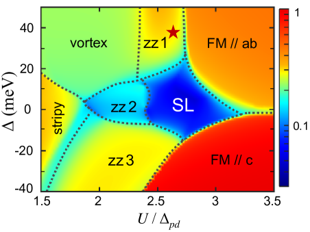
Figure 1: The calculated magnetic phase diagram of honeycomb cobaltates. The Kitaev SL phase is surrounded by ferromagnetic (FM) states with moments in the honeycomb $ab$-plane and along the $c$-axis, zigzag-type states with moments in the $ab$ plane (zz1), along Co-O bonds (zz2), and in the $ac$ plane (zz3). Vortex- and stripy-type phases take over at smaller $U/\Delta_{pd}$. The color map shows the second-NN spin correlation strength (leading eigenvalue of the correlation matrix $\langle\widetilde{S}^{\alpha}_{i}\widetilde{S}^{\beta}_{j}\rangle$ normalized by $\widetilde{S}^{2}=1/4$), which drops sharply in the SL phase. The star indicates the rough position of Na₃Co₂SbO₆.

Our main results are summarized in Fig. 1, displaying various magnetic phases of spin-orbit entangled pseudospin-1/2 Co²⁺ ions on a honeycomb lattice. The phase diagram is shown as a function of trigonal field $\Delta$, in a window relevant for honeycomb cobaltates, and a ratio of Coulomb repulsion $U$ and the charge-transfer gap $\Delta_{pd}$ Zaa85 . From the analysis of experimental data, we find that Na₃Co₂SbO₆ Vic07_m ; Won16_m ; Yan19_m is located at just $\sim 20$ meV “distance” from the Kitaev SL phase (see Fig. 1), and could be driven there by a $c$-axis compression that reduces $\Delta$. This seems feasible, given that $\Delta$ variations within a window of $\sim 70$ meV were achieved by strain control in a cobalt oxide Csi05 .

We now describe our calculations resulting in Fig. 1. In short, we first derive the pseudospin exchange interactions from a microscopic theory, as a function of various parameters, and then obtain the corresponding ground states numerically by exact diagonalization.

Exchange interactions.– In an octahedral environment, Co²⁺ ion with $t_{2g}^{5}e_{g}^{2}$ configuration possesses spin $S=3/2$ and effective orbital moment $L=1$, which form, via spin-orbit coupling, a pseudospin $\widetilde{S}=1/2$ Abr70_m . Over decades, cobaltates served as a paradigm for quantum magnetism, providing a variety of pseudospin-1/2 models ranging from the Heisenberg model in perovskites with corner-sharing octahedra Hol71 ; Buy71 to the Ising model when the CoO₆ octahedra share their edges Col10 .

A microscopic theory of Co²⁺ interactions in the edge-sharing geometry has been developed just recently Liu18_m ; San18 , assuming an ideal cubic symmetry. Here we consider a realistic case of trigonally distorted lattices, where $t_{2g}$ orbitals split as shown in Fig. 2(a). Our goal is to see if such distortions leave enough room for the Kitaev model physics in real compounds. This is decided by the spin-orbital structure of the pseudospin $\widetilde{S}=1/2$ wave functions; in terms of $|S_{Z},L_{Z}\rangle$ states (the trigonal axis $Z\!\parallel\!c$ is perpendicular to the honeycomb plane), they read as:

$$\Big{|}\!\pm\widetilde{\frac{1}{2}}\Big{\rangle}=\mathcal{C}_{1}\Big{|}\pm\frac{3}{2},\mp 1\Big{\rangle}+\mathcal{C}_{2}\Big{|}\pm\frac{1}{2},0\Big{\rangle}+\mathcal{C}_{3}\Big{|}\mp\frac{1}{2},\pm 1\Big{\rangle}.$$ (1)

The coefficients $\mathcal{C}_{1,2,3}$ depend on a relative strength $\Delta/\lambda$ of the trigonal field $\Delta(L^{2}_{Z}-\tfrac{2}{3})$ and SOC $\lambda\bm{L}\cdot\bm{S}$ Lin63_m ; SM . At $\Delta=0$, one has $(\mathcal{C}_{1},\mathcal{C}_{2},\mathcal{C}_{3})=(\tfrac{1}{\sqrt{2}},\tfrac{-1}{\sqrt{3}},\tfrac{1}{\sqrt{6}})$, and all the three components of $\bm{L}$ are equally active. A positive (negative) $\Delta$ field tends to quench $L_{Z}$ ($L_{X/Y}$).

The next step is to project various spin-orbital exchange interactions in cobaltates Liu18_m onto the above pseudospin-1/2 subspace. The calculations are standard but very lengthy; the readers interested in details are referred to the Supplemental Material SM . At the end, we obtain the $\widetilde{S}=1/2$ Kitaev model $K\widetilde{S}_{i}^{\gamma}\widetilde{S}_{j}^{\gamma}$, supplemented by Heisenberg $J$ and off-diagonal anisotropy $\Gamma,\Gamma^{\prime}$ terms; for $\gamma=z$ type NN bonds, they read as:

$$\mathcal{H}_{ij}^{(z)}=K\widetilde{S}_{i}^{z}\widetilde{S}_{j}^{z}+J\widetilde{\bm{S}}_{i}\cdot\widetilde{\bm{S}}_{j}+\Gamma(\widetilde{S}_{i}^{x}\widetilde{S}_{j}^{y}+\widetilde{S}_{i}^{y}\widetilde{S}_{j}^{x} )$$

$$+\;\Gamma^{\prime}(\widetilde{S}_{i}^{x}\widetilde{S}_{j}^{z}+\widetilde{S}_{i}^{z}\widetilde{S}_{j}^{x}+\widetilde{S}_{i}^{y}\widetilde{S}_{j}^{z}+\widetilde{S}_{i}^{z}\widetilde{S}_{j}^{y} ).$$ (2)

Interactions $\mathcal{H}_{ij}^{(\gamma)}$ for $\gamma=x,y$ type bonds follow from a cyclic permutation among $\widetilde{S}_{j}^{x}$, $\widetilde{S}_{j}^{y}$, and $\widetilde{S}_{j}^{z}$.

While the Hamiltonian (2) is of the same form as in $d^{5}$ Ir/Ru systems Win17_m ; Cha15_m , the microscopic origin of its parameters $K,J,\Gamma,\Gamma^{\prime}$ is completely different in $d^{7}$ Co compounds. This is due to the spin-active $e_{g}$ electrons of Co$(t_{2g}^{5}e_{g}^{2})$ ions, which generate new spin-orbital exchange channels $t_{2g}$-$e_{g}$ and $e_{g}$-$e_{g}$, shown in Fig. 2(b), in addition to the $t_{2g}$-$t_{2g}$ ones operating in $d^{5}$ systems with $t_{2g}$-only electrons. In fact, the new terms make a major contribution to the exchange parameters, as illustrated in Figs. 2(c)-2(f). In particular, Kitaev coupling $K$ comes almost entirely from the $t_{2g}$-$e_{g}$ process. It is also noticed that $t_{2g}$-$e_{g}$ and $e_{g}$-$e_{g}$ contributions to $J$, $\Gamma$, and $\Gamma^{\prime}$ are of opposite signs and largely cancel each other, resulting in only small overall values of these couplings.

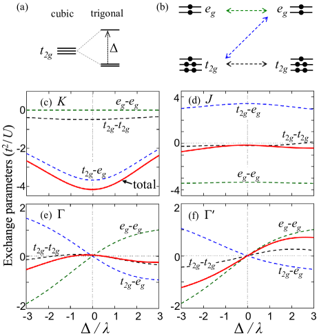
Figure 2: (a) Splitting of $t_{2g}$-electron level under trigonal crystal field. (b) Schematic of the spin-orbital exchange channels for $d^{7}$ ions. (c)-(f) Exchange parameters $K$, $J$, $\Gamma$, and $\Gamma^{\prime}$ (red solid lines) as a function of $\Delta/\lambda$, calculated at $U/\Delta_{pd}=2.5$ and Hund’s coupling $J_{H}=0.15U$. On each panel, dashed lines show individual contributions of $t_{2g}$-$t_{2g}$ (black), $t_{2g}$-$e_{g}$ (blue), and $e_{g}$-$e_{g}$ (green) exchange channels. The couplings $J$, $\Gamma$, and $\Gamma^{\prime}$ nearly vanish in the cubic limit $\Delta=0$.

Figure 2 shows that the trigonal field $\Delta$, which acts via modification of the pseudospin wavefunction (1), has an especially strong impact on the non-Kitaev couplings $J$, $\Gamma$, $\Gamma^{\prime}$. As a result, the relative strength ($J/K$, etc) of these “undesired” terms is very sensitive to $\Delta$ variations. This suggests the orbital splitting $\Delta$ as an efficient (and experimentally accessible) parameter that controls the proximity of cobaltates to the Kitaev-model regime.

Another important parameter in the theory is the $U/\Delta_{pd}$ ratio. In contrast to Ir/Ru-based Mott insulators with small $U/\Delta_{pd}\sim 0.5$, cobaltates are charge-transfer insulators Zaa85 , with typical values of $U/\Delta_{pd}\sim 2-3$ depending on the material chemistry. Including both Mott-Hubbard $U$ and charge-transfer $\Delta_{pd}$ excitations, we have calculated SM the exchange couplings as a function of $U/\Delta_{pd}$ and $\Delta/\lambda$. Figure 3(a) shows that Kitaev coupling $K$ is not much sensitive to $U/\Delta_{pd}$ variations. On the other hand, the non-Kitaev terms, especially Heisenberg coupling $J$, are quite sensitive to $U/\Delta_{pd}$, see Figs. 3(b)-3(d). However, their values relative to $K$ remain small over a broad range of parameters.

Phase diagram.– Having quantified the exchange parameters in Hamiltonian (2), we are now ready to address the corresponding ground states. As Kitaev coupling is the leading term, the model is highly frustrated. We therefore employ exact diagonalization (ED) which has been widely used to study phase behavior of the extended Kitaev-Heisenberg models (see, e.g., Refs. Cha10 ; Cha13_m ; Oka13 ; Rau14 ; Cha16_m ; Rus19_m ). In particular, by utilizing the method of coherent spin states Cha16_m ; Rus19_m , we can detect and identify the magnetically ordered phases (including easy-axis directions for the ordered moments). When non-Kitaev couplings are small (roughly below $10\%$ of the FM $K$ value), a quantum spin-liquid state is expected. Reflecting the unique feature of the Kitaev model Kit06 , this state is characterized by short-range spin correlations that are vanishingly small beyond nearest-neighbors Cha10 .

The resulting phase diagram, along with the data quantifying spin correlations beyond NN distances, is presented in Figs. 3(e) and 3(f). The main trends in the phase map are easy to understand considering the variations of non-Kitaev couplings with $\Delta/\lambda$ and $U/\Delta_{pd}$. As we see in Figs. 3(c) and 3(d), $\Gamma^{\prime}$ exactly vanishes at the $\Delta=0$ line, and $\Gamma$ is very small too. Thus, in the cubic limit, the model (2) essentially becomes the well studied $K-J$ model, with large FM Kitaev $K$ term, and $J$ correction changing from AF $J>0$ to FM $J<0$ as a function of $U/\Delta_{pd}$. Consequently, the ground state changes from stripy AF (at small $U/\Delta_{pd}$) to FM order at large $U/\Delta_{pd}$, through the Kitaev SL phase in between Cha13_m . In the SL phase, spin correlations are indeed short-ranged and bond-selective: for $z$-type NN bonds, we find $\langle\widetilde{S}^{z}\widetilde{S}^{z}\rangle/\widetilde{S}^{2}\simeq 0.52$ (as in the Kitaev model), while they nearly vanish at farther distances, see Figs. 3(e) and 3(f).

As we switch on the trigonal field $\Delta$, the $\Gamma^{\prime}$ term comes into play confining the SL phase to the window of $|\Delta|/\lambda<1$ (where $|\Gamma^{\prime}/K|<0.1$). In the FM phases, the sign of $\Gamma^{\prime}$ decides the direction of the FM moments. On the left-top (left-bottom) part of the phase map, where Heisenberg coupling $J$ is AF, the stripy state gives way to a vortex-type Cha15_m (zigzag-type) ordering, stabilized by the combined effect of $\Gamma$ and $\Gamma^{\prime}$ terms.

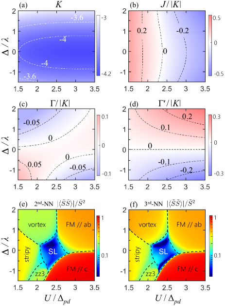
Figure 3: (a) Kitaev coupling $K$ (in units of $t^{2}/U$), and (b)-(d) the relative values of $J/|K|$, $\Gamma/|K|$, and $\Gamma^{\prime}/|K|$ as a function of $\Delta/\lambda$ and $U/\Delta_{pd}$. For convenience, specific values of parameters are indicated by contour lines. (e)-(f) The corresponding phase diagram obtained by ED of the model on a hexagon-shaped 24-site cluster. As in Fig. 1, the color maps quantify the strength of (e) second-NN and (f) third-NN spin correlations, which drop sharply in the SL phase (small but finite values are due to deviations from the pure Kitaev model Cha10 ).

To summarize up to now, the nearest-neighbor pseudospin Hamiltonian is dominated by the FM Kitaev model, which appears to be robust against trigonal splitting of orbitals. Subleading terms, represented mostly by $J$ and $\Gamma^{\prime}$ couplings, shape the phase diagram, which includes a sizeable SL area. While these observations are encouraging, it is crucial to inspect how the picture is modified by longer range interactions, especially by the third-NN Heisenberg coupling $J_{3}\widetilde{\bm{S}}_{i}\cdot\widetilde{\bm{S}}_{j}$, which appears to be one of the major obstacles on the way to a Kitaev SL in 5$d$ and 4$d$ compounds Win16_m ; Win17_m . We have no reliable estimate for $J_{3}$, since long-range interactions involve multiple exchange channels and are thus sensitive to material chemistry details. As such, they have to be determined experimentally. We note that $|J_{3}/K|\simeq 0.1$ was estimated Win18 ; Win17a in the 4$d$ compound RuCl₃; in cobaltates with more localized 3$d$ orbitals note_r2 , this ratio is expected to be smaller.

Adding a $J_{3}$ term to the model (2), we have re-examined the ground states and found that the Kitaev SL phase is stable up to $|J_{3}/K|\sim 0.06$ SM . The modified phase diagram, obtained for a representative value of $J_{3}=0.15t^{2}/U\simeq 0.04|K|$, is shown in Fig. 1 note_axis . Its comparison with Fig. 3 tells that the main effect of $J_{3}$ is to support the zigzag-type states (with different orientation of moments) at the expense of other phases. Note also that the SL area is shifted to the right, where FM $J$ and AF $J_{3}$ tend to frustrate each other. The phase diagram in Fig. 1 should be generic to Co²⁺ honeycomb systems, and will be used in the following discussion.

Honeycomb lattice cobaltates.– A number of such compounds are known: $A_{3}$Co₂SbO₆ ($A$=Na,Ag,Li) Vic07_m ; Won16_m ; Yan19_m ; Zve16_m ; Str19_m , Na₂Co₂TeO₆ Vic07_m ; Lef16_m ; Ber17_m ; Yao19_m , BaCo₂($X$O₄)₂ ($X$=As, P) Reg06_m ; Zho19_m ; Nai18_m ; Zho18_m , CoTiO₃ New64_m ; Bal17_m ; Yua19_m , CoPS₃ Bre86_m ; Wil17_m . They are quasi-two-dimensional magnets; within the $ab$-planes, zigzag or FM order is most common.

Traditionally, experimental data in Co²⁺ compounds is analysed in terms of an effective $\widetilde{S}=1/2$ models of $XXZ$ type Hut73_m ; Reg06_m ; Tom11_m ; Ros17_m ; Nai18_m ; Yua19_m . As $\widetilde{S}=1/2$ magnons ($\sim 10$ meV) are well separated from higher lying spin-orbit excitations ($\sim 30$ meV), the pseudospin picture itself is well justified; however, a conventional $XXZ$ model neglects the bond-directional nature of pseudospin $\widetilde{S}=1/2$ interactions. A general message of our work is that a proper description of magnetism in cobaltates should be based on the model of Eq. (2), supplemented by longer-range interactions. We note in passing that the $XXZ$ model also follows from Eq. (2) when the Kitaev-type anisotropy is suppressed Cha15_m ; however, such an extreme limit is unlikely for realistic trigonal fields, given the robustness of the $K$ coupling, see Fig. 3.

As an example, we consider Na₃Co₂SbO₆ which has low Néel temperature and a reduced ordered moment Yan19_m . Analysing the magnetic susceptibility data Yan19_m including all spin-orbit levels SM , we obtain a positive trigonal field $\Delta\simeq 38$ meV and $\lambda\simeq 28$ meV; these values are typical for Co²⁺ ions in an octahedral environment (see, e.g., Ref. Yua19_m ). With $\Delta/\lambda\simeq 1.36$, we evaluate $\widetilde{S}=1/2$ doublet $g$-factors $g_{ab}\simeq 4.6$ and $g_{c}\simeq 3$, from which a saturated moment of $2.3\mu_{B}$, consistent with the magnetization data Yan19_m , follows.

Zigzag-ordered moments in Na₃Co₂SbO₆ are confined to the $ab$ plane Yan19_m ; this corresponds to the zz1 phase in Fig. 1. The easy-plane anisotropy is due to the $\Gamma^{\prime}$ term, which is positive for $\Delta>0$, see Fig. 3(d). Regarding the location of Na₃Co₂SbO₆ on the $U/\Delta_{pd}$ axis of Fig. 1, we believe it is close to the FM/​/$ab$ phase, based on the following observations. First, a sister compound Li₃Co₂SbO₆ has $ab$-plane FM order Str19_m (most likely due to smaller Co-O-Co bond angle, $91^{\circ}$ versus $93^{\circ}$, slightly enhancing the FM $J$ value). Second, zigzag order gives way to fully polarized state at small magnetic fields Vic07_m ; Yan19_m . These facts imply that zz1 and FM/​/$ab$ states are closely competing in Na₃Co₂SbO₆.

Based on the above considerations, we roughly locate Na₃Co₂SbO₆ in the phase diagram as shown in Fig. 1. In this parameter area, the exchange couplings are $K\simeq-3.6\;t^{2}/U$, $J/|K|\sim-0.14$, $\Gamma/|K|\sim-0.03$, and $\Gamma^{\prime}/|K|\sim 0.16$, see Figs. 3(a)-3(d). The small values of $J,\Gamma,\Gamma^{\prime}$ imply the proximity to the Kitaev model, explaining a strong reduction of the ordered moments from their saturated values Yan19_m . As a crucial test for our theory, we show in Fig. 4 the expected spin excitations. The large FM Kitaev interaction enhances magnon spectral weight near $\bm{q}=0$ and leads to its anisotropy in momentum space, see Figs. 4(a) and 4(b). The ED results in Fig. 4(c) show that, as a consequence of the dominant Kitaev coupling, magnons are strongly renormalized and only survive at low energies, and a broad continuum of excitations Win17a ; Goh17 as in RuCl₃ Ban18 ; San15 emerges. Neutron scattering experiments on Na₃Co₂SbO₆ are desired to verify these predictions.

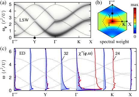
Figure 4: Spin excitation spectrum expected in Na₃Co₂SbO₆. The parameters $K=-3.6$, $J=-0.5$, $\Gamma=-0.1$, $\Gamma^{\prime}=0.6$ (in units of $t^{2}/U$) follow from our theory, while $J_{3}=0.15$ is added “by hand” note_J3 to stabilize the zigzag order. (a) Magnon dispersions and intensities from linear spin wave (LSW) theory. (b) The energy-integrated magnon intensity over the Brillouin zone. The intensity is largest around $\Gamma$, i.e. away from the Bragg point Y. (c) Exact diagonalization results for hexagonal 24- and 32-site clusters. Plotted is the trace $\chi^{\prime\prime}(\bm{q},\omega)$ of the spin susceptibility tensor SM , which comprises the low-energy magnon peak and a broad continuum.

If the above picture is confirmed by experiments, the next step should be to drive Na₃Co₂SbO₆ into the Kitaev SL state. As suggested by Fig. 1, this requires a reduction of the trigonal field by $\sim 20$ meV, e.g. by means of strain or pressure control. At this point, the relative smallness of SOC for 3$d$ Co ions comes as a great advantage: while strong enough to form the pseudospin moments, it makes the lattice manipulation of the $\widetilde{S}=1/2$ wave functions (and hence magnetism) far easier than in iridates Liu19 . Monitoring the magnetic behavior of Na₃Co₂SbO₆ and other honeycomb cobaltates under uniaxial pressure would be thus very interesting.

To conclude, we have presented a comprehensive theory of exchange interactions in honeycomb cobaltates, and studied their magnetic phase behavior. The analysis of Na₃Co₂SbO₆ data suggests that this compound is proximate to a Kitaev SL phase and could be driven there by a $c$-axis compression. A broader message is that as one goes from 5$d$ Ir to 4$d$ Ru and further to 3$d$ Co, magnetic $d$ orbitals become more localized, and this should improve the conditions for realization of the nearest-neighbor-only interaction model designed by Kitaev.

We thank A. Yaresko, T. Takayama, and A. Smerald for discussions, and M. Songvilay for sharing unpublished data. G.Kh. acknowledges support by the European Research Council under Advanced Grant No. 669550 (Com4Com). J.Ch. acknowledges support by Czech Science Foundation (GAČR) under Project No. GA19-16937S and MŠMT ČR under NPU II project CEITEC 2020 (LQ1601). Computational resources were supplied by the project “e-Infrastruktura CZ” (e-INFRA LM2018140) provided within the program Projects of Large Research, Development and Innovations Infrastructures.

Supplemental Material for
Kitaev Spin Liquid in $3d$ Transition Metal Compounds

SI I. Single-ion wavefunctions

The $d^{7}$ Co²⁺ ions in an octahedral crystal field have predominantly $t_{2g}^{5}e_{g}^{2}$ configuration with a high spin $S=3/2$ Abr70 . A trigonal distortion along $Z$-axis splits the $t_{2g}$ manifold into an orbital singlet $a_{1g}$ and a doublet $e_{g}^{\prime}$ by energy $\Delta$, see Fig. S1(a,b). In the electron representation, it is captured by the Hamiltonian $H_{\Delta}=\tfrac{1}{3}\Delta(2n_{a_{1g}}-n_{e^{\prime}_{g}})$. In terms of the effective angular momentum $L=1$ of the Co²⁺ ions, the $a_{1g}$-hole configuration corresponds to $L_{Z}=0$, while the $e_{g}^{\prime}$ doublet hosts the $L_{Z}=\pm 1$ states. Consequently, the trigonal field Hamiltonian translates into $H_{\Delta}=\Delta(L_{Z}^{2}-\tfrac{2}{3})$. The following relations between the $L$-states and orbitals hold:

$$|L_{Z}=0\rangle =\frac{1}{\sqrt{3}}\left(|a\rangle+|b\rangle+|c\rangle\right),$$

$$|L_{Z}=\pm 1\rangle =\pm\frac{1}{\sqrt{3}}\left(e^{\pm i\tfrac{2\pi}{3}}|a\rangle+e^{\mp i\tfrac{2\pi}{3}}|b\rangle+|c\rangle\right),$$ (S1)

where shorthand notations $a=d_{yz}$, $b=d_{zx}$, and $c=d_{xy}$ are used.

Diagonalization of $H_{\Delta}=\Delta(L_{Z}^{2}-\tfrac{2}{3})$ and $H_{\lambda}=\lambda\bm{L}\cdot\bm{S}$ results in a level structure shown in Fig. S1(c). The states are labeled according to the total angular momentum $J_{\rm eff}=\widetilde{\frac{1}{2}}$, $\widetilde{\frac{3}{2}}$, and $\widetilde{\frac{5}{2}}$. The ground state Kramers doublet hosts a pseudospin $\widetilde{S}=1/2$; its wavefunctions, written in the basis of $|S_{Z},L_{Z}\rangle$, read as:

$$\Big{|}\!\widetilde{\frac{1}{2}},\pm\widetilde{\frac{1}{2}}\Big{\rangle}=\mathcal{C}_{1}\Big{|}\pm\frac{3}{2},\mp 1\Big{\rangle}+\mathcal{C}_{2}\Big{|}\pm\frac{1}{2},0\Big{\rangle}+\mathcal{C}_{3}\Big{|}\mp\frac{1}{2},\pm 1\Big{\rangle}.$$ (S2)

The coefficients obey a relation $\mathcal{C}_{1}:\mathcal{C}_{2}:\mathcal{C}_{3}=\frac{\sqrt{6}}{r_{1}}:-1:\frac{\sqrt{8}}{r_{1}+2}$, where the parameter $r_{1}>0$ is determined by the equation $\frac{\Delta}{\lambda}=\frac{r_{1}+3}{2}-\frac{3}{r_{1}}-\frac{4}{r_{1}+2}$ Lin63 . The ground state energy is

$$E_{\rm GS}=\frac{\Delta}{3}-\frac{\lambda}{2}(r_{1}+3).$$ (S3)

The exchange Hamiltonian between the pseudospins $\widetilde{S}=1/2$ is obtained by projecting the Kugel-Khomskii type spin-orbital Hamiltonians onto the ground state doublet (S2).

We also specify the excited states, which will be needed in Sec. IV to calculate the magnetic susceptibility. The wavefunctions and energies for $\Big{|}\!\widetilde{\frac{3}{2}},\pm\widetilde{\frac{1}{2}}\Big{\rangle}$ and $\Big{|}\!\widetilde{\frac{5}{2}},\pm\widetilde{\frac{1}{2}}\Big{\rangle}$ states share the same form as of Eq. S2 and Eq. S3, but with different $r_{1}$. Namely, the above equation $\frac{\Delta}{\lambda}=\frac{r_{1}+3}{2}-\frac{3}{r_{1}}-\frac{4}{r_{1}+2}$ has three roots. The root $r_{1}>0$ corresponds to the ground state. The other two roots with $-2<r_{1}<0$ and $r_{1}<-2$ correspond to $\Big{|}\!\widetilde{\frac{3}{2}},\pm\widetilde{\frac{1}{2}}\Big{\rangle}$ and $\Big{|}\!\widetilde{\frac{5}{2}},\pm\widetilde{\frac{1}{2}}\Big{\rangle}$ states, respectively. The wavefunctions and energies of the remaining states are:

$$\Big{|}\!\widetilde{\frac{3}{2}},\pm\widetilde{\frac{3}{2}}\Big{\rangle}=c_{\varphi}\Big{|}\pm\frac{3}{2},0\Big{\rangle}-s_{\varphi}\Big{|}\pm\frac{1}{2},\pm 1\Big{\rangle}\;, E(\!\widetilde{\tfrac{3}{2}},\pm\widetilde{\tfrac{3}{2}})=-\tfrac{1}{2}\sqrt{\left(\Delta+\tfrac{1}{2}\lambda\right)^{2}+6\lambda^{2}}+\tfrac{1}{4}\lambda-\tfrac{1}{6}\Delta\;,$$

$$\Big{|}\!\widetilde{\frac{5}{2}},\pm\widetilde{\frac{3}{2}}\Big{\rangle}=s_{\varphi}\Big{|}\pm\frac{3}{2},0\Big{\rangle}+c_{\varphi}\Big{|}\pm\frac{1}{2},\pm 1\Big{\rangle}\;, E(\!\widetilde{\tfrac{5}{2}},\pm\widetilde{\tfrac{3}{2}})=\tfrac{1}{2}\sqrt{\left(\Delta+\tfrac{1}{2}\lambda\right)^{2}+6\lambda^{2}}+\tfrac{1}{4}\lambda-\tfrac{1}{6}\Delta\;,$$

$$\Big{|}\!\widetilde{\frac{5}{2}},\pm\widetilde{\frac{5}{2}}\Big{\rangle}=\Big{|}\pm\frac{3}{2},\pm 1\Big{\rangle}\;, E(\!\widetilde{\tfrac{5}{2}},\pm\widetilde{\tfrac{5}{2}})=\tfrac{3}{2}\lambda+\tfrac{2}{3}\Delta\;.$$ (S4)

Here, $c_{\varphi}=\cos\varphi$, $s_{\varphi}=\sin\varphi$, and $\tan 2\varphi=2\sqrt{6}\lambda/(2\Delta+\lambda)$.

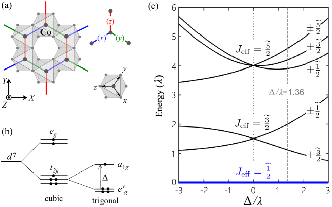
Figure S1: (a) Top view of the honeycomb cobaltate plane, $x$, $y$, and $z$ type NN-bonds are shown in blue, green, and red colors, respectively. The definition of global $X$, $Y$, $Z$ and the local cubic $x$, $y$, $z$ axes are shown in insets. (b) High-spin $d^{7}(t_{2g}^{5}e_{g}^{2})$ configuration in the trigonal crystal field $\Delta$. (c) Splitting of $S=3/2$, $L=1$ manifold of Co²⁺ ion under spin-orbit coupling $\lambda$ and trigonal field $\Delta$. At $\Delta/\lambda=1.36$ (appropriate for Na₃Co₂SbO₆), the first excited state energy is about $\lambda\sim 30$ meV.

SII II. Pseudospin $\widetilde{S}=1/2$ Hamiltonian and calculation of its parameters

In the cubic reference frame, pseudospin-1/2 interactions on $z$-type bonds have a general form

$$\mathcal{H}_{ij}^{(z)}=K\widetilde{S}_{i}^{z}\widetilde{S}_{j}^{z}+J\widetilde{\bm{S}}_{i}\cdot\widetilde{\bm{S}}_{j}+\Gamma(\widetilde{S}_{i}^{x}\widetilde{S}_{j}^{y}+\widetilde{S}_{i}^{y}\widetilde{S}_{j}^{x})+\Gamma^{\prime}(\widetilde{S}_{i}^{x}\widetilde{S}_{j}^{z}+\widetilde{S}_{i}^{z}\widetilde{S}_{j}^{x}+\widetilde{S}_{i}^{y}\widetilde{S}_{j}^{z}+\widetilde{S}_{i}^{z}\widetilde{S}_{j}^{y})\;.$$ (S5)

The interactions on $x$ and $y$ type bonds are obtained by cyclic permutations among $\widetilde{S}_{j}^{x}$, $\widetilde{S}_{j}^{y}$, and $\widetilde{S}_{j}^{z}$.

The Hamiltonian in Eq. S5 can also be written in global $XYZ$ reference frame Cha15 :

$$\mathcal{H}_{ij}^{(\gamma)}= J_{XY}\left(\widetilde{S}_{i}^{X}\widetilde{S}_{j}^{X}+\widetilde{S}_{i}^{Y}\widetilde{S}_{j}^{Y}\right)+J_{Z}\widetilde{S}_{i}^{Z}\widetilde{S}_{j}^{Z}$$

$$+ A\left[c_{\gamma}\left(\widetilde{S}_{i}^{X}\widetilde{S}_{j}^{X}-\widetilde{S}_{i}^{Y}\widetilde{S}_{j}^{Y}\right)-s_{\gamma}\left(\widetilde{S}_{i}^{X}\widetilde{S}_{j}^{Y}+\widetilde{S}_{i}^{Y}\widetilde{S}_{j}^{X}\right)\right]$$

$$- B\sqrt{2}\left[c_{\gamma}\left(\widetilde{S}_{i}^{X}\widetilde{S}_{j}^{Z}+\widetilde{S}_{i}^{Z}\widetilde{S}_{j}^{X}\right)+s_{\gamma}\left(\widetilde{S}_{i}^{Y}\widetilde{S}_{j}^{Z}+\widetilde{S}_{i}^{Z}\widetilde{S}_{j}^{Y}\right)\right],$$ (S6)

with $c_{\gamma}\equiv\cos\phi_{\gamma}$ and $s_{\gamma}\equiv\sin\phi_{\gamma}$. The angles $\phi_{\gamma}=0,\tfrac{2\pi}{3},\tfrac{4\pi}{3}$ refer to the $z$, $x$, and $y$ type bonds, respectively. The transformations between the two sets of parameters entering Eq. S5 and Eq. S6 are:

$$J_{XY}=J+\tfrac{1}{3}K-\tfrac{1}{3}(\Gamma+2\Gamma^{\prime})\;, K=A+2B\;,$$

$$J_{Z}=J+\tfrac{1}{3}K+\tfrac{2}{3}(\Gamma+2\Gamma^{\prime})\;, J=\tfrac{1}{3}(2J_{XY}+J_{Z}-A-2B)\;,$$

$$A=\tfrac{1}{3}K+\tfrac{2}{3}(\Gamma-\Gamma^{\prime})\;, \Gamma=\tfrac{2}{3}(A-B)+\tfrac{1}{3}(J_{Z}-J_{XY})\;,$$

$$B=\tfrac{1}{3}K-\tfrac{1}{3}(\Gamma-\Gamma^{\prime})\;, \Gamma^{\prime}=\tfrac{1}{3}(J_{Z}-J_{XY}+B-A)\;.$$ (S7)

Since the pseudospin wavefunctions (S2) are defined in the trigonal $XYZ$ basis, it is technically simpler to derive $\widetilde{S}=1/2$ Hamiltonian in a form of (S6), and then convert the results onto a cubic $xyz$ reference frame via Eqs. S7.

As discussed in the main text, there are three basic exchange channels in $d^{7}$ systems, which we consider now in detail. General form of the Kugel-Khomskii type spin-orbital Hamiltonians were obtained earlier Liu18 ; for completeness, they will be reproduced below. Here, the major task is to derive the corresponding pseudospin-1/2 Hamiltonians in a realistic case of finite trigonal splitting of $t_{2g}$ orbitals. As the $\widetilde{S}=1/2$ wavefunctions (S2) are somewhat complicated, the calculations are tedious but can still be done analytically.

SII.1 1. $t_{2g}$-$t_{2g}$ exchange contributions

SII.1.1 1.1 Intersite $U$ processes

The spin-orbital Hamiltonian for these exchange processes is given by equations (A2) and (3) of Ref. Liu18 :

$$\mathcal{H}^{(z)}_{11}= \frac{4t^{2}}{9}\frac{1}{E_{1}}(\bm{S}_{i}\cdot\bm{S}_{j}+S^{2})(a_{i}^{{\dagger}}b_{i}a_{j}^{{\dagger}}b_{j}+b_{i}^{{\dagger}}a_{i}b_{j}^{{\dagger}}a_{j})$$

$$+ \frac{4t^{2}}{27}\left(\frac{1}{E_{3}}+\frac{2}{E_{2}}\right)(\bm{S}_{i}\cdot\bm{S}_{j}+S^{2})(n_{ia}n_{jb}+n_{ib}n_{ja})$$

$$- \frac{t^{2}}{6}\left(\frac{1}{E_{1}}\!-\!\frac{1}{E_{2}}\right)(\bm{S}_{i}\cdot\bm{S}_{j}\!+\!S^{2})\left[(n_{ia}\!-\!n_{jb})^{2}\!+\!(n_{ib}\!-\!n_{ja})^{2}\right]$$

$$- \frac{4t^{2}}{27}\left(\frac{1}{E_{2}}-\frac{1}{E_{3}}\right)(\bm{S}_{i}\cdot\bm{S}_{j}-S^{2})(a_{i}^{{\dagger}}b_{i}b_{j}^{{\dagger}}a_{j}+b_{i}^{{\dagger}}a_{i}a_{j}^{{\dagger}}b_{j})$$

$$+ \frac{t^{2}}{6}\left(\frac{3}{E_{1}}+\frac{1}{E_{2}}-\frac{4}{E_{3}}\right)(n_{ia}n_{jb}+n_{ib}n_{ja})$$

$$- \frac{4}{9}\frac{tt^{\prime}}{U}(\bm{S}_{i}\cdot\bm{S}_{j}+S^{2})\left[(a_{i}^{{\dagger}}c_{i}c_{j}^{{\dagger}}b_{j}+c_{i}^{{\dagger}}a_{i}b_{j}^{{\dagger}}c_{j})+(a\leftrightarrow b)\right]$$

$$+ \frac{4}{9}\frac{t^{\prime 2}}{U}(\bm{S}_{i}\cdot\bm{S}_{j}-S^{2})\;n_{ic}n_{jc}.$$ (S8)

Here $n_{a}=a^{{\dagger}}a$, etc. denote the orbital occupations, $t$ is the hopping between $a$ and $b$ orbitals via ligand ions, $t^{\prime}$ is the direct overlap of $c$ orbitals. The Mott-Hubbard excitation energies are $E_{1}=U-3J_{H}$, $E_{2}=U+J_{H}$, and $E_{3}=U+4J_{H}$, where $U$ and $J_{H}$ are Coulomb repulsion and Hund’s coupling on Co²⁺ ions.

Now, we need to express various combinations of the spin and orbital operators above in terms of the pseudospins $\widetilde{S}=1/2$ defined by Eq. S2. To this end, we have derived a general projection table, presented in subsection 4 below. Using this table, we obtain the pseudospin Hamiltonian in the form of Eq. S6, with the following exchange constants:

$$J^{XY}_{11}= \frac{4t^{2}}{27}\left(\frac{3}{E_{1}}-\frac{1}{E_{2}}+\frac{1}{E_{3}}\right)\left(2u_{4}^{2}+2u_{6}^{2}-\tfrac{13}{2}u_{5}^{2}\right)+\frac{t^{2}}{27}\left(\frac{9}{E_{1}}-\frac{1}{E_{2}}+\frac{4}{E_{3}}\right)\left(\tfrac{2}{9}u_{1}^{2}-u_{4}^{2}-\tfrac{1}{2}u_{5}^{2}\right)$$

$$- \frac{2t^{2}}{9}\left(\frac{1}{E_{1}}-\frac{1}{E_{2}}\right)u_{1}^{2}-\frac{4}{9}\frac{tt^{\prime}}{U}\left(4u_{6}^{2}-2u_{4}^{2}+\tfrac{13}{2}u_{5}^{2}\right)+\frac{4}{9}\frac{t^{\prime 2}}{U}\left(\tfrac{1}{9}u_{1}^{2}+u_{4}^{2}+\tfrac{1}{2}u_{5}^{2}\right),$$ (S9)

$$J^{Z}_{11}= \frac{4t^{2}}{27}\left(\frac{3}{E_{1}}-\frac{1}{E_{2}}+\frac{1}{E_{3}}\right)\left[2u_{7}^{2}+u_{3}^{2}-\tfrac{3}{8}(u_{2}-1)^{2}\right]+\frac{t^{2}}{27}\left(\frac{9}{E_{1}}-\frac{1}{E_{2}}+\frac{4}{E_{3}}\right)\left(\tfrac{2}{9}u_{2}^{2}-2u_{3}^{2}\right)$$

$$- \frac{2t^{2}}{9}\left(\frac{1}{E_{1}}-\frac{1}{E_{2}}\right)u_{2}^{2}-\frac{4}{9}\frac{tt^{\prime}}{U}\left[4u_{7}^{2}-u_{3}^{2}-\tfrac{3}{4}(u_{2}-1)^{2}\right]+\frac{4}{9}\frac{t^{\prime 2}}{U}\left(\tfrac{1}{9}u_{2}^{2}+2u_{3}^{2}\right),$$

$$A_{11}= -\frac{4t^{2}}{27}\left(\frac{3}{E_{1}}-\frac{1}{E_{2}}+\frac{1}{E_{3}}\right)\left(4u_{4}u_{6}+\tfrac{13}{2}u_{5}^{2}\right)+\frac{t^{2}}{27}\left(\frac{9}{E_{1}}-\frac{1}{E_{2}}+\frac{4}{E_{3}}\right)\left(\tfrac{2}{3}u_{1}u_{4}+u_{5}^{2}\right)$$

$$- \frac{t^{2}}{3}\left(\frac{1}{E_{1}}-\frac{1}{E_{2}}\right)u_{1}u_{4}-\frac{4}{9}\frac{tt^{\prime}}{U}\left(4u_{4}u_{6}-13u_{5}^{2}\right)+\frac{4}{9}\frac{t^{\prime 2}}{U}\left(\tfrac{1}{2}u_{5}^{2}-\tfrac{2}{3}u_{1}u_{4}\right),$$

$$B_{11}= \frac{4t^{2}}{27}\left(\frac{3}{E_{1}}-\frac{1}{E_{2}}+\frac{1}{E_{3}}\right)\left[u_{3}(u_{6}-u_{4})-\frac{u_{5}}{\sqrt{2}}\left(u_{7}-\tfrac{9}{4}u_{2}+\tfrac{9}{4}\right)\right]+\frac{t^{2}}{27}\left(\frac{9}{E_{1}}-\frac{1}{E_{2}}+\frac{4}{E_{3}}\right)\left[u_{3}\left(\tfrac{1}{3}u_{1}+2u_{4}\right)-\tfrac{1}{3\sqrt{2}}u_{2}u_{5}\right]$$

$$- \frac{t^{2}}{6}\left(\frac{1}{E_{1}}-\frac{1}{E_{2}}\right)\!\left(u_{1}u_{3}-\tfrac{1}{\sqrt{2}}u_{2}u_{5}\right)+\frac{4}{9}\frac{tt^{\prime}}{U}\left[u_{3}(2u_{4}+u_{6})-\frac{u_{5}}{\sqrt{2}}\left(u_{7}-\tfrac{9}{4}u_{2}+\tfrac{9}{4}\right)\right]-\frac{4}{9}\frac{t^{\prime 2}}{U}\!\left[u_{3}\left(\tfrac{1}{3}u_{1}-u_{4}\right)-\tfrac{1}{3\sqrt{2}}u_{2}u_{5}\right].$$

Coefficients $u_{i}$ ($i=1,2,\ldots,7$) are given by Eqs. SII.4 below; they depend on the spatial shape of the pseudospin wavefunctions (S2), and thus decide how the relative values of the pseudospin interactions vary as a function of trigonal field $\Delta$.

SII.1.2 1.2 Charge-transfer processes

The spin-orbital Hamiltonian is (Eq. 9 in Ref. Liu18 ):

$$\mathcal{H}^{(z)}_{12} =\frac{4}{9}\frac{t^{2}}{\Delta_{pd}+\frac{U_{p}}{2}}(\bm{S}_{i}\cdot\bm{S}_{j}-S^{2})(n_{ia}n_{jb}+n_{ib}n_{ja})-\frac{2}{9}\frac{t^{2}\;J^{p}_{H}}{(\Delta_{pd}+\frac{U^{\prime}_{p}}{2})^{2}}\;\bm{S}_{i}\cdot\bm{S}_{j}(n_{ic}+n_{jc}),$$ (S10)

where $\Delta_{pd}$ is charge-transfer gap. $U_{p}$ and $U^{\prime}_{p}=U_{p}-2J^{p}_{H}$ are the intra- and inter-orbital Coulomb repulsion of the ligand $p$ orbitals, respectively, and $J^{p}_{H}$ is the Hund’s coupling.

Using the projection table of subsection 4, we find the exchange constants in the form of Eq. S6:

$$J^{XY}_{12} =\frac{4}{9}\frac{t^{2}}{\Delta_{pd}+\frac{U_{p}}{2}}\left(\tfrac{2}{9}u_{1}^{2}-u_{4}^{2}-\tfrac{1}{2}u_{5}^{2}\right)-\frac{4}{27}\frac{t^{2}\;J^{p}_{H}}{(\Delta_{pd}+\frac{U^{\prime}_{p}}{2})^{2}}\;u_{1}^{2}\;,$$

$$J^{Z}_{12} =\frac{4}{9}\frac{t^{2}}{\Delta_{pd}+\frac{U_{p}}{2}}\left(\tfrac{2}{9}u_{2}^{2}-2u_{3}^{2}\right)-\frac{4}{27}\frac{t^{2}\;J^{p}_{H}}{(\Delta_{pd}+\frac{U^{\prime}_{p}}{2})^{2}}\;u_{2}^{2}\;,$$

$$A_{12} =\frac{4}{9}\frac{t^{2}}{\Delta_{pd}+\frac{U_{p}}{2}}\left(\tfrac{2}{3}u_{1}u_{4}+u_{5}^{2}\right)+\frac{4}{9}\frac{t^{2}\;J^{p}_{H}}{(\Delta_{pd}+\frac{U^{\prime}_{p}}{2})^{2}}\;u_{1}u_{4}\;,$$

$$B_{12} =\frac{4}{9}\frac{t^{2}}{\Delta_{pd}+\frac{U_{p}}{2}}\left[u_{3}\left(\tfrac{1}{3}u_{1}+2u_{4}\right)-\tfrac{1}{3\sqrt{2}}u_{2}u_{5}\right]+\frac{2}{9}\frac{t^{2}\;J^{p}_{H}}{(\Delta_{pd}+\frac{U^{\prime}_{p}}{2})^{2}}\;\left(u_{1}u_{3}-\tfrac{1}{\sqrt{2}}u_{2}u_{5}\right).$$ (S11)

SII.1.3 1.3 Cyclic exchange processes

The spin-orbital Hamiltonian is (Eq. 11 in Ref. Liu18 ):

$$\mathcal{H}^{(z)}_{13}=\frac{4}{9}\frac{t^{2}}{\Delta_{pd}}(\bm{S}_{i}\cdot\bm{S}_{j}+S^{2})(a_{i}^{{\dagger}}b_{i}a_{j}^{{\dagger}}b_{j}+b_{i}^{{\dagger}}a_{i}b_{j}^{{\dagger}}a_{j}).$$ (S12)

After projection, we obtain the exchange constants as:

$$J^{XY}_{13} =\frac{4}{9}\frac{t^{2}}{\Delta_{pd}}\left(2u_{4}^{2}+2u_{6}^{2}-\tfrac{13}{2}u_{5}^{2}\right), \quad\ \ \ \ \ \ \ \ \ \ \ \ \ J^{Z}_{13} =\frac{4}{9}\frac{t^{2}}{\Delta_{pd}}\left[2u_{7}^{2}+u_{3}^{2}-\tfrac{3}{8}(u_{2}-1)^{2}\right],$$

$$A_{13} =-\frac{4}{9}\frac{t^{2}}{\Delta_{pd}}\left(4u_{4}u_{6}+\tfrac{13}{2}u_{5}^{2}\right), B_{13} =\frac{4}{9}\frac{t^{2}}{\Delta_{pd}}\left[u_{3}(u_{6}-u_{4})-\frac{u_{5}}{\sqrt{2}}\left(u_{7}-\tfrac{9}{4}u_{2}+\tfrac{9}{4}\right)\right].$$ (S13)

The total contribution from $t_{2g}$-$t_{2g}$ hopping channel to Eq. S6 is given by

$$J^{XY}_{1} =J^{XY}_{11}+J^{XY}_{12}+J^{XY}_{13}\;, \quad\ \ \ \ \ \ \ \ \ \ \ \ \ J^{Z}_{1} =J^{Z}_{11}+J^{Z}_{12}+J^{Z}_{13}\;,$$

$$A_{1} =A_{11}+A_{12}+A_{13}\;, B_{1} =B_{11}+B_{12}+B_{13}\;.$$ (S14)

The corresponding $K$, $J$, $\Gamma$, and $\Gamma^{\prime}$ values can be obtained using Eqs. S7.

SII.2 2. $t_{2g}$-$e_{g}$ exchange contributions

SII.2.1 2.1 Intersite $U$ processes

The corresponding spin-orbital exchange Hamiltonian is (Eq. A5 in Ref. Liu18 ):

$$\mathcal{H}^{(z)}_{21} =\frac{4\alpha_{1}}{9}\frac{tt_{e}}{\widetilde{U}}(\bm{S}_{i}\cdot\bm{S}_{j}-S^{2})(n_{ic}+n_{jc})-\frac{tt_{e}}{6}\frac{\Delta_{e}}{\Delta_{pd}}\left(\frac{1}{E_{1}+D}\!-\!\frac{1}{E_{2}+D}\right)\bm{S}_{i}\cdot\bm{S}_{j}\;(2-n_{ic}-n_{jc}).$$ (S15)

Here, $t_{e}=t_{pd\sigma}^{2}/\Delta_{e}$, with $t_{pd\sigma}$ representing hopping between $p$ and $e_{g}$ orbitals via the charge-transfer gap $\Delta_{e}=\Delta_{pd}+D$. Parameter $D$ is the splitting between $t_{2g}$ and $e_{g}$ levels. The constants $\alpha_{1}$ and $1/\widetilde{U}$ are:

$$\alpha_{1}=1-\frac{D^{2}}{2\Delta_{pd}\Delta_{e}}\left(\frac{\Delta_{pd}+\Delta_{e}}{U+2J_{H}}-1\right),\ \ \ \ \ \ \ \ \ \ \ \ \ \frac{1}{\widetilde{U}}=\frac{1}{6}\left(\frac{2}{E_{2}+D}\!+\!\frac{1}{E_{3}+D}\!+\!\frac{3}{U+2J_{H}-D}\right).$$ (S16)

After projection onto pseudospin-1/2 doublet (S2), we get the exchange constants in the form of Eq. S6:

$$J^{XY}_{21} =\left[\frac{8\alpha_{1}}{27}\frac{tt_{e}}{\widetilde{U}}-\frac{2tt_{e}}{9}\frac{\Delta_{e}}{\Delta_{pd}}\left(\frac{1}{E_{1}+D}\!-\!\frac{1}{E_{2}+D}\right)\right]u_{1}^{2}\;,$$

$$J^{Z}_{21} =\left[\frac{8\alpha_{1}}{27}\frac{tt_{e}}{\widetilde{U}}-\frac{2tt_{e}}{9}\frac{\Delta_{e}}{\Delta_{pd}}\left(\frac{1}{E_{1}+D}\!-\!\frac{1}{E_{2}+D}\right)\right]u_{2}^{2}\;,$$

$$A_{21} =-\left[\frac{8\alpha_{1}}{9}\frac{tt_{e}}{\widetilde{U}}+\frac{tt_{e}}{3}\frac{\Delta_{e}}{\Delta_{pd}}\left(\frac{1}{E_{1}+D}\!-\!\frac{1}{E_{2}+D}\right)\right]u_{1}u_{4}\;,$$

$$B_{21} =\left[\frac{4\alpha_{1}}{9}\frac{tt_{e}}{\widetilde{U}}+\frac{tt_{e}}{6}\frac{\Delta_{e}}{\Delta_{pd}}\left(\frac{1}{E_{1}+D}\!-\!\frac{1}{E_{2}+D}\right)\right]\left(\frac{u_{2}u_{5}}{\sqrt{2}}-u_{1}u_{3}\right).$$ (S17)

SII.2.2 2.2 Charge-transfer processes

The spin-orbital Hamiltonian describing these processes is (Eq. 19 in Ref. Liu18 ):

$$\mathcal{H}^{(z)}_{22} =\frac{8\alpha_{2}}{9}\frac{tt_{e}}{\Delta_{pd}+\frac{U_{p}}{2}}(\bm{S}_{i}\cdot\bm{S}_{j}-S^{2})(n_{ic}+n_{jc})-\frac{2\alpha_{3}}{9}\frac{tt_{e}\;J^{p}_{H}}{(\Delta_{pd}+\frac{D+U^{\prime}_{p}}{2})^{2}}\;\bm{S}_{i}\cdot\bm{S}_{j}\;(2-n_{ic}-n_{jc}),$$ (S18)

where

$$\alpha_{2}=1-\frac{D}{4(\Delta_{e}+\frac{U_{p}}{2})}+\frac{D\;U_{p}}{8\Delta_{pd}(\Delta_{e}+\frac{U_{p}}{2})}-\frac{D}{4\Delta_{e}},\ \ \ \ \ \ \ \ \ \ \ \alpha_{3}=\frac{(\Delta_{pd}+\Delta_{e})^{2}}{4\Delta_{pd}\Delta_{e}}\;.$$ (S19)

The corresponding pseudospin exchange constants are:

$$J^{XY}_{22} =\left[\frac{16\alpha_{2}}{27}\frac{tt_{e}}{\Delta_{pd}+\frac{U_{p}}{2}}-\frac{8\alpha_{3}}{27}\frac{tt_{e}\;J^{p}_{H}}{(\Delta_{pd}+\frac{D+U^{\prime}_{p}}{2})^{2}}\right]u_{1}^{2}\;,$$

$$J^{Z}_{22} =\left[\frac{16\alpha_{2}}{27}\frac{tt_{e}}{\Delta_{pd}+\frac{U_{p}}{2}}-\frac{8\alpha_{3}}{27}\frac{tt_{e}\;J^{p}_{H}}{(\Delta_{pd}+\frac{D+U^{\prime}_{p}}{2})^{2}}\right]u_{2}^{2}\;,$$

$$A_{22} =-\left[\frac{16\alpha_{2}}{9}\frac{tt_{e}}{\Delta_{pd}+\frac{U_{p}}{2}}+\frac{4\alpha_{3}}{9}\frac{tt_{e}\;J^{p}_{H}}{(\Delta_{pd}+\frac{D+U^{\prime}_{p}}{2})^{2}}\right]u_{1}u_{4}\;,$$

$$B_{22} =\left[\frac{8\alpha_{2}}{9}\frac{tt_{e}}{\Delta_{pd}+\frac{U_{p}}{2}}+\frac{2\alpha_{3}}{9}\frac{tt_{e}\;J^{p}_{H}}{(\Delta_{pd}+\frac{D+U^{\prime}_{p}}{2})^{2}}\right]\left(\frac{u_{2}u_{5}}{\sqrt{2}}-u_{1}u_{3}\right).$$ (S20)

SII.2.3 2.3 Cyclic exchange processes

The corresponding spin-orbital Hamiltonian is (Eq. 22 in Ref. Liu18 ):

$$\mathcal{H}^{(z)}_{23}=-\frac{2\alpha_{4}}{9}\frac{tt_{e}}{\Delta_{pd}}(\bm{S}_{i}\cdot\bm{S}_{j}+S^{2})(n_{ic}+n_{jc}),$$ (S21)

with $\alpha_{4}=1-\frac{1}{2}\frac{D}{\Delta_{pd}+D}$.

After projection onto pseudospin-1/2 doublet, we obtain:

$$J^{XY}_{23}=-\frac{4\alpha_{4}}{27}\frac{tt_{e}}{\Delta_{pd}}u_{1}^{2}\;, J^{Z}_{23}=-\frac{4\alpha_{4}}{27}\frac{tt_{e}}{\Delta_{pd}}u_{2}^{2}\;,$$

$$A_{23}=\frac{4\alpha_{4}}{9}\frac{tt_{e}}{\Delta_{pd}}u_{1}u_{4}\;, B_{23}=-\frac{2\alpha_{4}}{9}\frac{tt_{e}}{\Delta_{pd}}\left(\frac{u_{2}u_{5}}{\sqrt{2}}-u_{1}u_{3}\right).$$ (S22)

The total contribution from $t_{2g}$-$e_{g}$ exchange channel to Eq. S6 is given by

$$J^{XY}_{2} =J^{XY}_{21}+J^{XY}_{22}+J^{XY}_{23}\;, \quad\ \ \ \ \ \ \ \ \ \ \ \ \ J^{Z}_{2} =J^{Z}_{21}+J^{Z}_{22}+J^{Z}_{23}\;,$$

$$A_{2} =A_{21}+A_{22}+A_{23}\;, \quad\ \ \ \ \ \ \ \ \ \ \ \ \ B_{2} =B_{21}+B_{22}+B_{23}\;.$$ (S23)

SII.3 3. $e_{g}$-$e_{g}$ exchange contribution

The corresponding Hamiltonian is very simple (see Eq. 27 in Ref. Liu18 ):

$$\mathcal{H}^{(z)}_{3}=-\frac{4}{9}\frac{t^{2}_{e}\;J^{p}_{H}}{(\Delta_{e}+\frac{U^{\prime}_{p}}{2})^{2}}\;\bm{S}_{i}\cdot\bm{S}_{j}.$$ (S24)

Note that no orbital operators are involved in this interaction and thus it has no bond-dependence. This is because $e_{g}$ doublet hosts two electrons with parallel spins, leaving no $e_{g}$-orbital degeneracy. After projecting Eq. S24 onto pseudospin subspace, we find

$$J^{XY}_{3}=-\frac{4}{9}\frac{t^{2}_{e}\;J^{p}_{H}}{(\Delta_{e}+\frac{U^{\prime}_{p}}{2})^{2}}u_{1}^{2}\;,\ \ \ \ \ \ \ \ \ \ \ J^{Z}_{3}=-\frac{4}{9}\frac{t^{2}_{e}\;J^{p}_{H}}{(\Delta_{e}+\frac{U^{\prime}_{p}}{2})^{2}}u_{2}^{2}\;,$$ (S25)

while the bond-dependent terms $A_{3}=B_{3}=0$. The latter implies that $e_{g}$-$e_{g}$ interaction channel supports the $XXZ$-type model. In the cubic reference frame, Eq. S5, this translates into $K=0$ and $\Gamma=\Gamma^{\prime}$.

Total values of the exchange constants are obtained by summing up $t_{2g}$-$t_{2g}$, $t_{2g}$-$e_{g}$, and $e_{g}$-$e_{g}$ contributions [Eqs. S14, S23, and S25, respectively], and converted into $K$, $J$, $\Gamma$, and $\Gamma^{\prime}$ using Eqs. S7.

SII.4 4. Projection table

Calculating the matrix elements of spin-orbital operators within the pseudospin $\widetilde{S}=1/2$ doublet (S2), we obtain the correspondence:

$$S_{+}=u_{1}\widetilde{S}_{+}\;,\ \ \;S_{-}=u_{1}\widetilde{S}_{-}\;,\ \ \;S_{Z}=u_{2}\widetilde{S}_{Z}\;,\ \ \;$$ (S26)

$$S_{+}n_{a} =\sqrt{2}u_{3}e^{i\tfrac{2\pi}{3}}\widetilde{S}_{Z}+\frac{u_{1}}{3}\widetilde{S}_{+}-u_{4}e^{i\tfrac{4\pi}{3}}\widetilde{S}_{-}\;,$$

$$S_{-}n_{a} =\sqrt{2}u_{3}e^{-i\tfrac{2\pi}{3}}\widetilde{S}_{Z}+\frac{u_{1}}{3}\widetilde{S}_{-}-u_{4}e^{-i\tfrac{4\pi}{3}}\widetilde{S}_{+}\;,$$

$$S_{Z}n_{a} =\frac{u_{2}}{3}\widetilde{S}_{Z}+\frac{u_{5}}{2}(\widetilde{S}_{X}-\sqrt{3}\widetilde{S}_{Y})\;,$$ (S27)

$$S_{+}n_{b} =\sqrt{2}u_{3}e^{-i\tfrac{2\pi}{3}}\widetilde{S}_{Z}+\frac{u_{1}}{3}\widetilde{S}_{+}-u_{4}e^{-i\tfrac{4\pi}{3}}\widetilde{S}_{-}\;,$$

$$S_{-}n_{b} =\sqrt{2}u_{3}e^{i\tfrac{2\pi}{3}}\widetilde{S}_{Z}+\frac{u_{1}}{3}\widetilde{S}_{-}-u_{4}e^{i\tfrac{4\pi}{3}}\widetilde{S}_{+}\;,$$

$$S_{Z}n_{b} =\frac{u_{2}}{3}\widetilde{S}_{Z}+\frac{u_{5}}{2}(\widetilde{S}_{X}+\sqrt{3}\widetilde{S}_{Y})\;,$$ (S28)

$$S_{+}n_{c} =\sqrt{2}u_{3}\widetilde{S}_{Z}+\frac{u_{1}}{3}\widetilde{S}_{+}-u_{4}\widetilde{S}_{-}\;,$$

$$S_{-}n_{c} =\sqrt{2}u_{3}\widetilde{S}_{Z}+\frac{u_{1}}{3}\widetilde{S}_{-}-u_{4}\widetilde{S}_{+}\;,$$

$$S_{Z}n_{c} =\frac{u_{2}}{3}\widetilde{S}_{Z}-u_{5}\widetilde{S}_{X}\;,$$ (S29)

$$a^{\dagger}b =\tfrac{i}{2\sqrt{3}}[(1-u_{2})\widetilde{S}_{Z}-6u_{5}\widetilde{S}_{X}]\;,\ \ \ \ \ \ \ \ S_{+}a^{\dagger}b=-\frac{u_{3}}{\sqrt{2}}\widetilde{S}_{Z}+u_{6}\widetilde{S}_{+}-u_{4}\widetilde{S}_{-}\;,$$

$$S_{-}a^{\dagger}b =-\frac{u_{3}}{\sqrt{2}}\widetilde{S}_{Z}+u_{6}\widetilde{S}_{-}-u_{4}\widetilde{S}_{+}\;,\ \ \ \ \ \ \ \ S_{Z}a^{\dagger}b=u_{7}\widetilde{S}_{Z}+\frac{u_{5}}{2}\widetilde{S}_{X}\;,$$ (S30)

$$b^{\dagger}c =\tfrac{i}{2\sqrt{3}}[(1-u_{2})\widetilde{S}_{Z}-3u_{5}(\sqrt{3}\widetilde{S}_{Y}-\widetilde{S}_{X})]\;,\ \ \ \ \ \ \ \ S_{+}b^{\dagger}c=\frac{u_{3}}{\sqrt{2}}e^{-i\tfrac{\pi}{3}}\widetilde{S}_{Z}+u_{6}\widetilde{S}_{+}-u_{4}e^{-i\tfrac{2\pi}{3}}\widetilde{S}_{-}\;,$$

$$S_{-}b^{\dagger}c =\frac{u_{3}}{\sqrt{2}}e^{i\tfrac{\pi}{3}}\widetilde{S}_{Z}+u_{6}\widetilde{S}_{-}-u_{4}e^{i\tfrac{2\pi}{3}}\widetilde{S}_{+}\;,\ \ \ \ \ \ \ \ S_{Z}b^{\dagger}c=u_{7}\widetilde{S}_{Z}-\frac{u_{5}}{4}(\widetilde{S}_{X}-\sqrt{3}\widetilde{S}_{Y})\;,$$ (S31)

$$c^{\dagger}a =\tfrac{i}{2\sqrt{3}}[(1-u_{2})\widetilde{S}_{Z}+3u_{5}(\sqrt{3}\widetilde{S}_{Y}+\widetilde{S}_{X})]\;,\ \ \ \ \ \ \ \ S_{+}c^{\dagger}a=\frac{u_{3}}{\sqrt{2}}e^{i\tfrac{\pi}{3}}\widetilde{S}_{Z}+u_{6}\widetilde{S}_{+}-u_{4}e^{i\tfrac{2\pi}{3}}\widetilde{S}_{-}\;,$$

$$S_{-}c^{\dagger}a =\frac{u_{3}}{\sqrt{2}}e^{-i\tfrac{\pi}{3}}\widetilde{S}_{Z}+u_{6}\widetilde{S}_{-}-u_{4}e^{-i\tfrac{2\pi}{3}}\widetilde{S}_{+}\;,\ \ \ \ \ \ \ \ S_{Z}c^{\dagger}a=u_{7}\widetilde{S}_{Z}-\frac{u_{5}}{4}(\widetilde{S}_{X}+\sqrt{3}\widetilde{S}_{Y})\;,$$ (S32)

The parameters $u_{i}$ ($i=1,2,\ldots,7$) are determined by the pseudospin wavefunction (S2) parameters $\mathcal{C}_{1,2,3}$ as:

$$u_{1} =2\sqrt{3}\mathcal{C}_{1}\mathcal{C}_{3}+2\mathcal{C}_{2}^{2}\;,\ \ \ \ \ \ u_{2}=1+2(\mathcal{C}_{1}^{2}-\mathcal{C}_{3}^{2})\;,\ \ \ \ \ \ u_{3}=\tfrac{2\sqrt{2}}{3}\mathcal{C}_{2}\mathcal{C}_{3}-\sqrt{\tfrac{2}{3}}\mathcal{C}_{1}\mathcal{C}_{2}\;,\ \ \ \ \ \ u_{4}=\tfrac{2}{3}\mathcal{C}_{3}^{2}\;,$$

$$u_{5} =\tfrac{2}{3}\mathcal{C}_{2}\mathcal{C}_{3}\;,\ \ \ \ \ \ \ \ \ \ \ \ \ \ \ \ \ \ u_{6}=\tfrac{2}{3}\mathcal{C}_{2}^{2}-\tfrac{1}{\sqrt{3}}\mathcal{C}_{1}\mathcal{C}_{3}\;,\ \ \ \ \ \ \ \ u_{7}=\tfrac{1}{3}\mathcal{C}_{2}^{2}+\tfrac{1}{6}\mathcal{C}_{3}^{2}-\tfrac{1}{2}\mathcal{C}_{1}^{2}\;.$$ (S33)

In the cubic limit, where $(\mathcal{C}_{1},\mathcal{C}_{2},\mathcal{C}_{3})=(\tfrac{1}{\sqrt{2}},\tfrac{-1}{\sqrt{3}},\tfrac{1}{\sqrt{6}})$, they are

$$u_{1}=u_{2}=\frac{5}{3}\;,\ \ \;u_{3}=u_{4}=\frac{1}{9}\;,\ \ \;u_{5}=-\frac{\sqrt{2}}{9}\;,\ \ \;u_{6}=\frac{1}{18}\;,\ \ \;u_{7}=-\frac{1}{9}\;.$$ (S34)

SII.5 5. Microscopic parameters used in the calculations

Apart from an overall energy scale $t^{2}/U$, a number of microscopic parameters appeared in the above expressions for exchange constants. Hund’s coupling $J_{H}\sim 0.8$ eV follows from optical data in CoO Pra59 ; cubic splitting $D$ for 3$d$ ions is of the order of $1.0-1.5$ eV. With the ab initio estimates of $U\sim 5.0-7.8$ eV Ani91 ; Pic98 ; Jia10 , this gives $J_{H}/U\sim 0.1-0.2$ and $D/U\sim 0.13-0.30$. Specifically, we set $J_{H}/U=0.15$ and $D/U=0.20$. Hund’s coupling on oxygen is large, $J_{H}^{p}\sim 1.2-1.6$ eV Foy13 , while $U_{p}$ is about $\sim 4$ eV, so we use the representative values of $J_{H}^{p}/U_{p}=0.3$ and $U_{p}/U=0.7$. We set a direct hopping $t^{\prime}=0.2t$ (i.e. smaller than in 5$d$/4$d$ compounds Win16 ), but this value is nearly irrelevant here since $t_{2g}$-$t_{2g}$ exchange is of minor importance anyway, see Fig. 2 of the main text. A ratio $t_{pd\sigma}/t_{pd\pi}=2$ Cha08 is used. Regarding $\Delta/\lambda$ and $U/\Delta_{pd}$ values, we vary them rather broadly, as they most sensitively control the exchange interactions. With the above input parameters, we arrive at $K$, $J$, $\Gamma$, and $\Gamma^{\prime}$ values presented in the main text. We have verified that while variations of the input parameters result in some changes of the exchange constants, they do not affect the overall picture and conclusions.

SIII III. Exact diagonalization: Phase diagrams based on static correlations and coherent-state analysis

We consider the nearest-neighbor (NN) interaction model (Eq. 2 of the main text or S5 in the previous section), supplemented by the third-NN Heisenberg exchange $J_{3}$ that appears as the major one among the long-range interactions in ab-initio studies Win16 . In this section we show the full evolution of the phase diagram with the parameter $J_{3}$ and also demonstrate the robustness of our picture with respect to variations of the Hund’s exchange $J_{H}$. The data presented here complements Fig. 1 and Fig. 3(e,f) of the main manuscript.

To determine the magnetic state, we have performed exact diagonalization using the values of exchange parameters derived in Sec. II. Utilizing the Lanczos method, we have obtained exact ground states of the exchange Hamiltonian for a symmetric, hexagon-shaped cluster containing 24 sites. Periodic boundary conditions were applied, corresponding to a periodic tiling of an infinite lattice. Since the small cluster does not allow for spontaneous symmetry breaking, we inspect its magnetic state by analyzing the static spin correlations and by employing the method of coherent spin states introduced in Ref. Cha16 .

We focus on real-space correlations that enable us to judge the extent of the Kitaev spin liquid phase which should be characterized by vanishing correlations beyond nearest neighbors. By evaluating the static spin correlations in momentum space, we would be able to detect the magnetically ordered states that show peaks at the characteristic momenta of the particular ordering pattern. Here, however, it is favorable to utilize the method of coherent spin states that provides a better access to the magnetic order encoded in the complex cluster wavefunction. In essence, it constructs “classical” states (coherent spin states) with spins pointing in prescribed directions and identifies a “classical” state having maximum overlap with the exact cluster ground state. Thanks to its full flexibility in the individual spin directions, the method can precisely determine both collinear patterns as well as non-collinear ones. The “classical” trial state is a product state of spins pointing in prescribed directions (in the sense of finding spin up with 100% probability when measuring in that particular direction) and as such it excludes quantum fluctuations. The maximum overlap is therefore a useful indicator of the amount of quantum fluctuations. For a fluctuation-free state and non-degenerate cluster ground state, the corresponding probability reaches the value $1/\text{(number of degenerate patterns)}$. In contrast, Kitaev spin liquid is highly fluctuating and does not contain a pronounced “classical” state which leads to a tiny maximum overlap (see Cha16 ; Rus19 for details).

Figures S3 and S4 show phase diagram data as functions of $U/\Delta_{pd}$ and $\Delta/\lambda$ for several values of $J_{3}$. The static correlations up to fourth NN presented in upper three rows of panels clearly localize the Kitaev spin liquid phase spreading in the area with dominant $K$. It is surrounded by several phases with long-range correlations that are identified by the method of coherent spin states. For $J_{3}=0$, these include two types of FM orders with the magnetic moments lying in the honeycomb plane and perpendicular to it, respectively, stripy phase, zigzag phase zz3, and finally a vortex phase of the type depicted in Fig. S2.

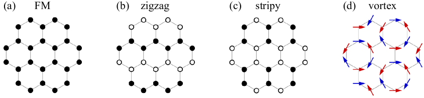
Figure S2: Sketch of the magnetic structures for (a) FM, (b) zigzag, (c) stripy, and (d) vortex orders. Open and closed circles represent opposite spin directions.

The effect of nonzero antiferromagnetic $J_{3}$ may be estimated by considering the correlations of third NN in the individual phases. Strongly supported by $J_{3}$ is the zigzag phase that is characterized by AF oriented spins on all third-neighbor bonds. Similarly, a large suppression may be expected for FM and stripy phases that have FM aligned third NN spins. The effect on the vortex phase is weak as each spin has one FM aligned third neighbor and two third neighbors at an angle of $120^{\circ}$, leading to a cancellation of $J_{3}$ in energy on classical level. Finally, in the Kitaev spin liquid phase the third neighbors are not correlated at all, so that small $J_{3}$ has a moderate negative impact when trying to align them in AF fashion. The consequences of the above energetics are well visible in Figs. S3 and S4. Once including nonzero $J_{3}$, the Kitaev spin liquid phase slightly grows first, at the expense of FM and stripy phases. At the same time, the Kitaev spin liquid phase is also being expelled from the bottom left corner by the expanding zz3 phase. With increasing $J_{3}$ between $J_{3}=0.05$ and $0.15$ in $t^{2}/U$ units, two new zigzag phases zz1 and zz2 around Kitaev SL are successively formed. Once $J_{3}$ reaches $0.25t^{2}/U$, the zigzag order quickly takes over, suppressing the Kitaev SL phase completely.

In the large area covered by the zigzag order, various ratios and combinations of signs of the nearest-neighbor interactions are realized. This is the origin of three distinct zigzag phases zz1, zz2, and zz3, differing in their moment directions as seen in bottom panels of Figs. S3 and S4. Negative $\Gamma$ and positive $\Gamma^{\prime}$ found in zz1 phase space [see Fig. 3(c,d) of the main text] lead to the $ab$-plane moment direction. The zz3 phase is characterized by opposite signs of $\Gamma$ and $\Gamma^{\prime}$ interactions which stabilizes the zigzag order as in Na₂IrO₃ Chu15 ; Cha16 . Finally, in the zz2 phase, $\Gamma$ and $\Gamma^{\prime}$ terms maintain only small values and moment directions pointing along cubic axes $x$, $y$, $z$ are selected by order-from-disorder mechanism Cha16 .

To check the robustness of our picture, we have also performed the exact diagonalization for a different $J_{H}$ value. The trends discussed above remain quite similar as demonstrated in Figs. S5 and S6 calculated for $J_{H}/U=0.2$. Roughly speaking, when we increase the $J_{H}/U$ value, the whole scenario merely shifts to smaller $U/\Delta_{pd}$ region.

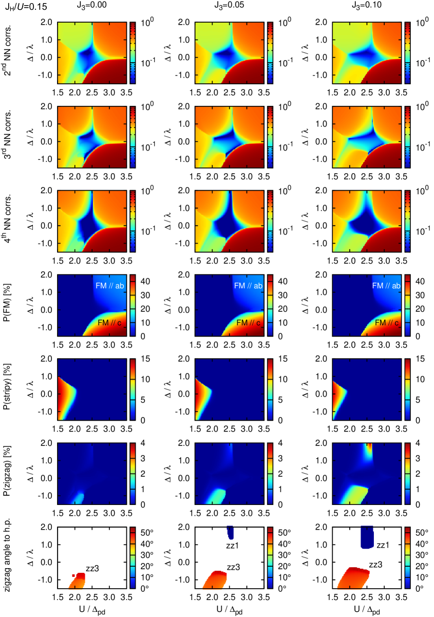
Figure S3: The first three rows present second-NN, third-NN and fourth-NN spin correlations. The color indicates the largest absolute value among the eigenvalues of the $3\times 3$ spin correlation matrix for the respective bond. It is normalized by the maximum possible value of $\widetilde{S}^{2}=0.25$. The next three rows are the probability of FM, stripy, and zigzag classical states contained in the cluster ground state as determined by the method of coherent spin states. The last row shows the angle between the honeycomb plane (h.p.) and the magnetic moments for the zigzag order. $J_{H}/U=0.15$ is fixed and three columns correspond to $J_{3}=0$, $J_{3}=0.05$, and $J_{3}=0.1$ in units of $t^{2}/U$.

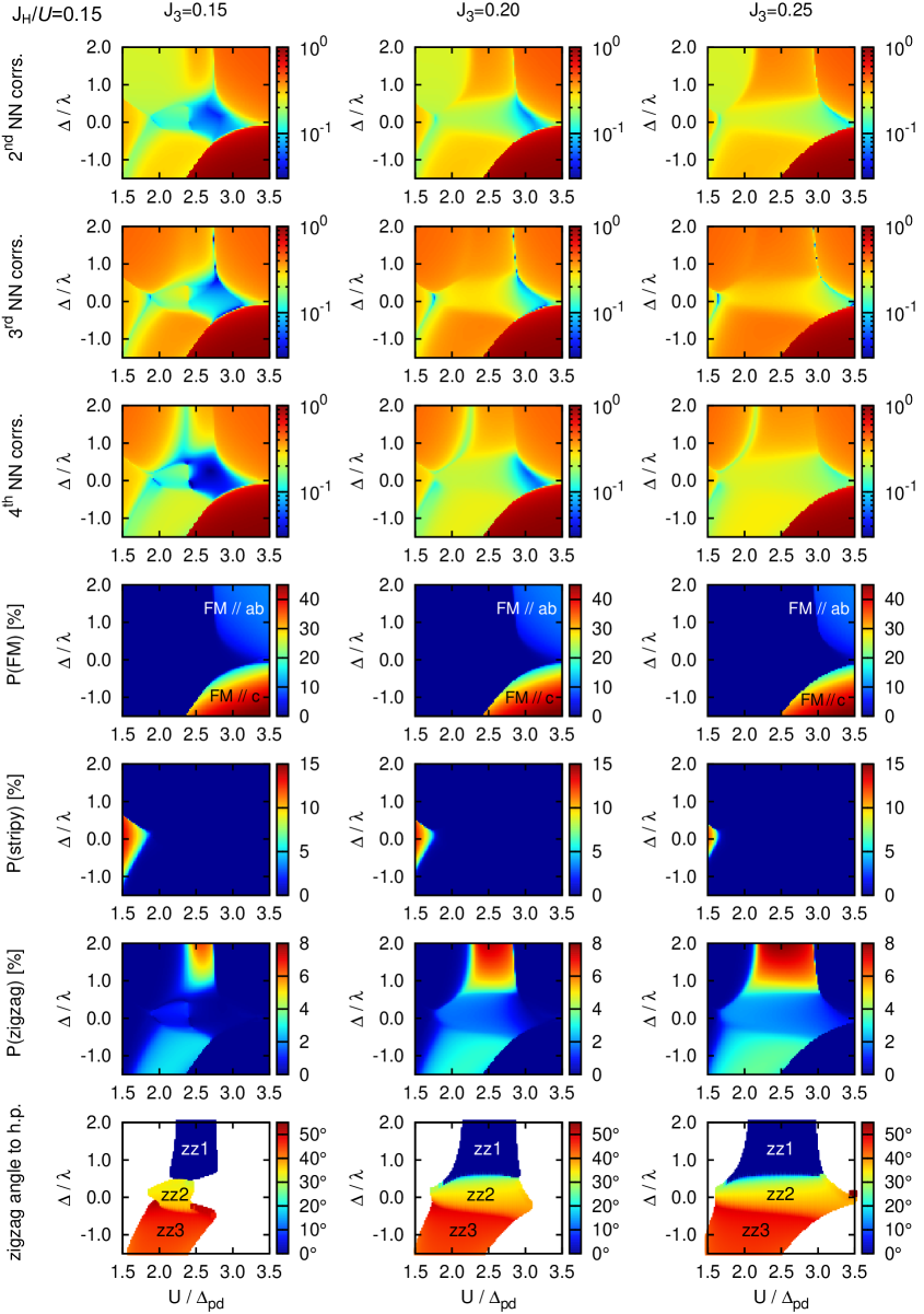
Figure S4: The same as in Fig. S3 for larger $J_{3}$ values. The three columns correspond to $J_{3}=0.15$, $0.20$, and $0.25$ ($t^{2}/U$).

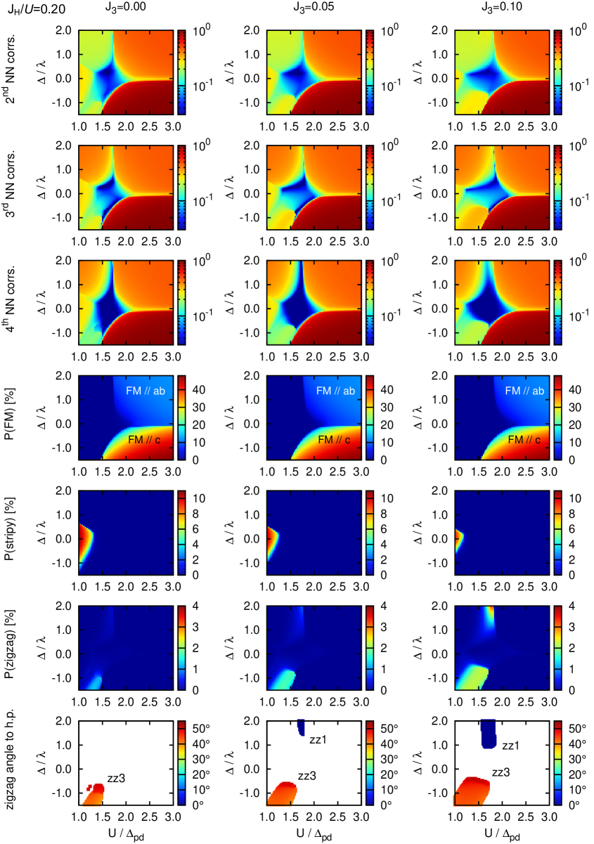
Figure S5: The same as in Fig. S3 for a larger value $J_{H}/U=0.2$. The three columns correspond to $J_{3}=0$, $J_{3}=0.05$, and $J_{3}=0.1$ ($t^{2}/U$).

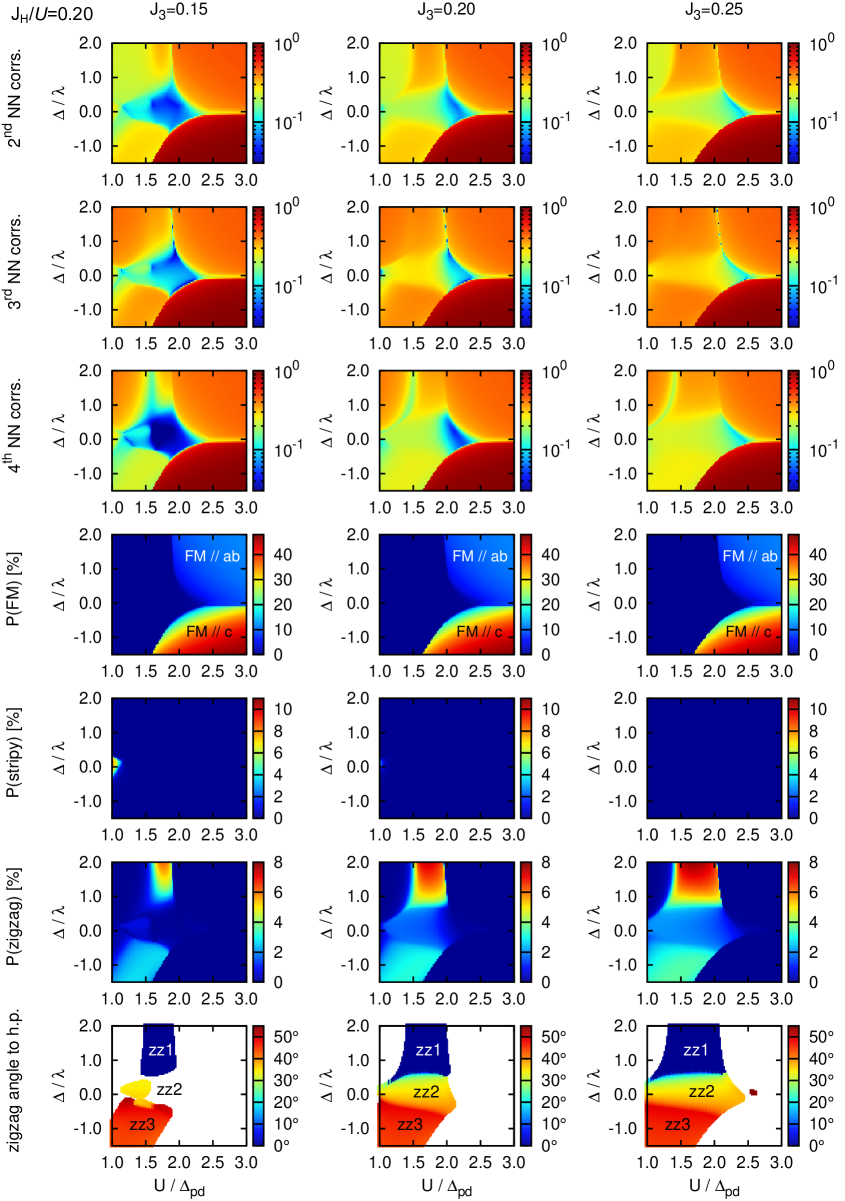
Figure S6: The same as in Fig. S5 for larger $J_{3}$ values. The three columns correspond to $J_{3}=0.15$, $0.20$, and $0.25$ ($t^{2}/U$).

SIV IV. Trigonal crystal field $\Delta$ in Na₃Co₂SbO₆

The parameter $\Delta$ determines the effective magnetic moment values $\mu^{\alpha}_{\rm eff}$ ($\alpha=ab$ or $c$), and thus can be obtained from paramagnetic susceptibility $\chi^{\alpha}(T)$. One has to keep in mind that extracting the moments from a standard Curie-Weiss fit $\chi(T)=C/(T-\Theta)+\chi_{0}$ assumes that the excited levels are high in energy (as compared to $k_{B}T$) and hence thermally unpopulated. The Curie constant $C$ is then indeed temperature independent, providing the ground state $g$-factors and moments. For Co²⁺ ions, where the excited level at $\sim 30$ meV is thermally activated already at the room temperature, we have to use instead a general expression for a single-ion susceptibility:

$$\chi^{\alpha}_{\rm ion}=\frac{1}{Z(T)}\sum_{n,m}\frac{e^{-\beta E_{n}}-e^{-\beta E_{m}}}{E_{m}-E_{n}}(M_{nm}^{\alpha})^{2}.$$ (S35)

Here, $n$ and $m$ run over all the 12 states (6 doublets in Fig. S1), with the wavefunctions and energies calculated in Sec. I. The partition function $Z(T)=\sum_{n}e^{-\beta E_{n}}$, and $\beta=1/k_{B}T$. $M_{nm}^{\alpha}=\langle n|M_{\alpha}|m\rangle$ is matrix element of the magnetic moment operator $\bm{M}=(2\bm{S}-\tfrac{3}{2}\kappa\bm{L})$ (in units of Bohr magneton $\mu_{B}$). We use the covalency reduction factor $\kappa=0.8$ typical for Co²⁺ ion Abr70 . $\chi^{\alpha}_{\rm ion}$ includes both the Curie and Van-Vleck contributions and depends on two parameters, $\Delta$ and $\lambda$.

We have fitted the data of Ref. Yan19 with $\chi^{\alpha}(T)=\chi^{\alpha}_{\rm ion}+\chi^{\alpha}_{0}$, and obtained a fair agreement with experiment for both $\chi^{ab}$ and $\chi^{c}$, using $\Delta=38$ meV and $\lambda=28$ meV, see Fig. S7(a,b). In particular, the characteristic changes in the slopes of both $1/\chi^{ab}$ and $1/\chi^{c}$ data are well reproduced by the calculations. In fact, this behavior is common for layered cobaltates and deserves some discussion.

It is instructive to divide Eq. S35 into two parts, $\chi^{\alpha}_{\rm ion}=\chi^{\alpha}_{1}+\chi^{\alpha}_{2}$, where $\chi^{\alpha}_{1}$ term accounts for the transitions within $\widetilde{S}=1/2$ doublet. Using the wavefunctions (S2), we obtain

$$\chi^{\alpha}_{1}=p_{1/2}\;\frac{(\mu^{\alpha}_{\rm eff})^{2}}{3k_{B}T}\;.$$ (S36)

The effective moments $\mu^{\alpha}_{\rm eff}=g_{\alpha}\sqrt{\widetilde{S}(\widetilde{S}+1)}$, with the $\widetilde{S}=1/2$ doublet $g$-factors given by

$$g_{ab} =4\sqrt{3}\mathcal{C}_{1}\mathcal{C}_{3}+4\mathcal{C}_{2}^{2}-3\sqrt{2}\kappa\mathcal{C}_{2}\mathcal{C}_{3}\;,$$

$$g_{c} =(6+3\kappa)\mathcal{C}_{1}^{2}+2\mathcal{C}_{2}^{2}-(2+3\kappa)\mathcal{C}_{3}^{2}\;.$$ (S37)

In Eq. S36, $p_{1/2}=2/Z(T)$ measures the occupation of the ground state. As the excited levels of Co²⁺ are relatively low, the weight $p_{1/2}$ of the Curie term, as well as Van-Vleck contribution $\chi^{\alpha}_{2}$ of the excited states depend on temperature. The characteristic changes in the slopes of $1/\chi^{ab}$ ($1/\chi^{c}$) around 200 K (100 K) originate from the interplay between $\chi_{1}(T)$ and $\chi_{2}(T)$ which become of a similar order at these temperatures, see Fig. S7(c,d).

The $g$-factors (S37) are plotted in Fig. S7(g); with $\Delta$ and $\lambda$ values obtained above, we get $g_{ab}\simeq$ 4.6 and $g_{c}\simeq$ 3. This gives the in-plane saturated magnetic moment $M_{ab}=g_{ab}\widetilde{S}=2.3\mu_{B}$ consistent with experiment Yan19 .

Apparent deviations at low temperatures are due to short-range correlations between the pseudospins, which can partially be accounted for in a molecular field approximation, i.e. replacing the Curie term $\chi^{\alpha}_{1}$ by $\chi^{\alpha}_{1}\cdot T/(T-\Theta_{\alpha})$. The result is shown in Fig. S7(e,f). The paramagnetic Curie temperatures $\Theta_{ab}=17$K and $\Theta_{c}=6$K are rather small and anisotropic. We can evaluate $\Theta$ values using our theoretical exchange constants given in Fig. 4 caption of the main text; the result is:

$$\Theta_{ab}=-\tfrac{3}{4}\left[J+J_{3}+\tfrac{1}{3}K-\tfrac{1}{3}(\Gamma+2\Gamma^{\prime})\right]\simeq 1.4\;(t^{2}/U),$$

$$\Theta_{c}=-\tfrac{3}{4}\left[J+J_{3}+\tfrac{1}{3}K+\tfrac{2}{3}(\Gamma+2\Gamma^{\prime})\right]\simeq 0.6\;(t^{2}/U).$$ (S38)

Curiously enough, this gives the $\Theta$-anisotropy close to what we get from the susceptibility fits. This comparison also suggests the energy scale of $t^{2}/U\sim 1$ meV, setting thereby the magnon bandwidth of the order of $10$ meV. The relative smallness of $t^{2}/U$ is due to large $U$ and more localized nature of $3d$ orbitals.

It is worth to comment on a positive sign of $\Delta>0$ in Na₃Co₂SbO₆. Within a simple model only considering contribution from $O_{6}$ octahedron, which is slightly compressed along the $c$-axis Yan19 , one would find a negative $\Delta<0$ instead. However, this approximation is too crude in layered structures, where the non-cubic Madelung potential of more distant ions has to be considered. In Na₃Co₂SbO₆, we think that $\Delta>0$ is due to a positive contribution of the high-valence $Sb^{5+}$ ions residing within the $ab$-plane. A $c$-axis compression would enhance a negative contribution of the oxygen octahedra, reducing thereby a total value of the trigonal field $\Delta$.

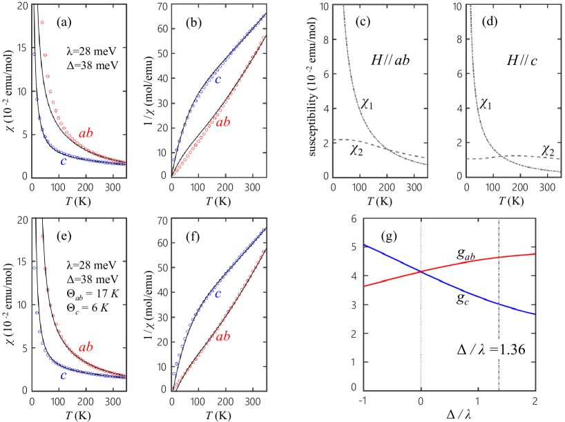
Figure S7: (a),(b) Temperature dependence of magnetic susceptibility $\chi$ and its inverse $1/\chi$ in Na₃Co₂SbO₆. Open circles represent the experimental data extracted from Ref. Yan19 , and solid lines are the fits using single-ion approximation $\chi^{\alpha}=\chi^{\alpha}_{\rm ion}+\chi^{\alpha}_{0}$, with $\chi^{ab}_{0}=-10^{-3}$ emu/mol and $\chi^{c}_{0}=1.5\times 10^{-3}$ emu/mol. (c),(d) Decomposition of single-ion susceptibility $\chi^{\alpha}_{\rm ion}$ into pseudospin-1/2 $\chi_{1}$ and Van-Vleck $\chi_{2}$ contributions. (e),(f) The fitting results including the pseudospin interactions within a molecular field approximation. Here, $\chi^{ab}_{0}=-1.5\times 10^{-3}$ emu/mol and $\chi^{c}_{0}=1.5\times 10^{-3}$ emu/mol. (g) The g-factors $g_{ab}$ (red) and $g_{c}$ (blue) as a function of $\Delta/\lambda$. $\Delta/\lambda=1.36$ corresponds to Na₃Co₂SbO₆.

SV V. Dynamical spin susceptibility

SV.1 1. Linear spin wave theory

The dispersions and intensitites of magnons presented in Fig. 4(a,b) of the main text were determined by standard linear spin wave (LSW) theory. Zigzag pattern with FM $x$ and $y$ bonds was assumed, i.e. the zigzags are running along the $X$ direction in Fig. S1(a). By applying Holstein-Primakoff transformation, harmonic expansion, and Bogoliubov transformation numerically, we have calculated diagonal components of the spin susceptibility tensor and evaluated its trace that is plotted in Fig. 4(a,b), including artificial lorentzian broadening with FWHM of $0.4$ in units of $t^{2}/U$.

SV.2 2. Exact diagonalization

The dynamical spin susceptibility profiles presented in Fig. 4(c) of the main text were determined by exact diagonalization (ED) using the hexagonal clusters with $N=24$ and $N=32$ sites shown in Fig. S8(a) and (b), respectively. Utilizing Lanczos algorithm, we have obtained the exact cluster ground state $|\mathrm{GS}\rangle$ and calculated the dynamical spin susceptibility tensor $\chi_{\alpha\beta}(\bm{q},\omega)=i\int\langle\mathrm{GS}|[S_{\bm{q}}^{\alpha}(t),S_{-\bm{q}}^{\beta}(0)]|\mathrm{GS}\rangle\exp(i\omega t)\theta(t)dt$. Here $S^{\alpha}_{\bm{q}}=\sum_{\bm{R}}S^{\alpha}_{\bm{R}}\exp(-i\bm{q}\bm{R})/\sqrt{N}$ is the Fourier component combining spin operators at cluster sites $\bm{R}$. The accessible wavevectors $\bm{q}$ that are compatible with periodic tiling of the honeycomb lattice by the clusters are depicted in Fig. S8(c). As in the case of the LSW theory, in Fig. 4(c) we have plotted the imaginary part of the trace of the spin susceptibility tensor: $\chi^{\prime\prime}(\bm{q},\omega)=\mathrm{Im}\sum_{\alpha}\chi_{\alpha\alpha}(\bm{q},\omega)$. The spectra were broadened by lorentzians with FWHM of $0.1$ in units of $t^{2}/U$ and the quasielastic peaks at momenta corresponding to the zigzag Bragg points were removed.

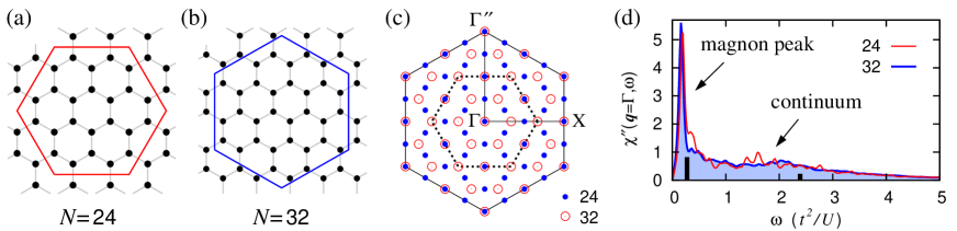
Figure S8: (a) 24-site cluster used in ED to obtain phase diagrams and spin susceptibility. (b) 32-site cluster used in ED calculations of the spin susceptibility. (c) Wavevectors compatible with the periodic tiling of the honeycomb lattice by 24- and 32-site clusters. Inner dotted hexagon indicates the Brillouin zone of the honeycomb lattice, outer hexagon corresponds to the Brillouin zone of the triangular lattice formed when adding sites at hexagon centers to the honeycomb lattice. (d) Imaginary part of the trace of the spin susceptibility tensor at $\bm{q}=\Gamma=0$ calculated by ED for 24- and 32-site clusters. The values of model parameters are the same as in Fig. 4 of the main text. The thick black bars show the positions and relative spectral weights of the magnon peaks obtained within LSW theory. Note that the ED results for 24- and 32-site clusters are qualitatively similar to each other.

Compared to the LSW approximation result, the ED profiles show highly renormalized magnons that only survive at low energies, and broad continua of excitations that emerge as a consequence of the dominant Kitaev interactions. In fact, the most spectral weight is taken by the continuum. This is illustrated in detail for the FM wavevector $\bm{q}=\Gamma=0$ in Fig. S8(d) and can be seen in Fig. 4(c) of the main text for other wavevectors $\bm{q}$ as well. To properly capture such broad continua, we have used 1000 Lanczos steps in the dynamical susceptibility evaluation.

Finally, we want to notice an important aspect that one has to keep in mind while comparing the above results with the experimental data. Namely, the cluster ground state is fully symmetric and contains all degenerate ordering patterns. In our case these correspond to the three possible zigzag directions that are represented with equal weights for the hexagonal shape clusters. As a result, the dynamical spin susceptibility obtained via ED contains contributions from all these zigzag patterns. In practice, this would correspond to the dynamical spin structure factor measured on the twinned samples with three types of zigzag domains. On the other hand, the intensities calculated using the LSW theory correspond to a single-domain crystal with one particular zigzag pattern.

References

(1) A. Kitaev, Ann. Phys. (N.Y.) 321, 2 (2006).
(2)
L. Savary and L. Balents, Rep. Prog. Phys. 80, 016502 (2017).
(3) M. Hermanns, I. Kimchi, and J. Knolle,
Annu. Rev. Condens. Matter Phys. 9, 17 (2018).
(4) S. Trebst, arXiv:1701.07056.
(5) S. M. Winter, A. A. Tsirlin, M. Daghofer, J. van den Brink,
Y. Singh, P. Gegenwart, and R. Valentí,
J. Phys.: Condens. Matter 29, 493002 (2017).
(6)
H. Takagi, T. Takayama, G. Jackeli, G. Khaliullin, and
S. E. Nagler, Nat. Rev. Phys. 1, 264 (2019).
(7)
Y. Motome and J. Nasu, J. Phys. Soc. Jpn. 89, 012002 (2020).
(8)
G. Khaliullin, Prog. Theor. Phys. Suppl. 160, 155 (2005).
(9)
G. Jackeli and G. Khaliullin, Phys. Rev. Lett. 102, 017205 (2009).
(10)
K.W. Plumb, J.P. Clancy, L.J. Sandilands, V.V. Shankar, Y.F. Hu, K.S. Burch,
H.-Y. Kee, and Y.-J. Kim,
Phys. Rev. B 90, 041112(R) (2014).
(11)
J. Chaloupka, G. Jackeli, and G. Khaliullin,
Phys. Rev. Lett. 105, 027204 (2010).
(12)
S. M. Winter, Y. Li, H. O. Jeschke, and R. Valentí,
Phys. Rev. B 93, 214431 (2016).
(13) Cf. and for Co2+ and Ru3+ ions (in a.u.), respectively Abr70 .
(14)
A. Abragam and B. Bleaney, Electron Paramagnetic
Resonance of Transition Ions (Clarendon Press, Oxford, 1970).
(15)
H. Liu and G. Khaliullin, Phys. Rev. B 97, 014407 (2018).
(16)
R. Sano, Y. Kato, and Y. Motome, Phys. Rev. B 97, 014408 (2018).
(17) J. Zaanen, G. A. Sawatzky, and J. W. Allen,
Phys. Rev. Lett. 55, 418 (1985).
(18) L. Viciu, Q. Huang, E. Morosan, H. W. Zandbergen,
N. I. Greenbaum, T. McQueen, and R. J. Cava,
J. Solid State Chem. 180, 1060 (2007).
(19) C. Wong, M. Avdeev, and C. D. Ling,
J. Solid State Chem. 243, 18 (2016).
(20)
J.-Q. Yan, S. Okamoto, Y. Wu, Q. Zheng, H. D. Zhou, H. B. Cao,
and M. A. McGuire,
Phys. Rev. Mater. 3, 074405 (2019).
(21)
S. I. Csiszar, M. W. Haverkort, Z. Hu, A. Tanaka, H. H. Hsieh,
H.-J. Lin, C. T. Chen, T. Hibma, and L. H. Tjeng,
Phys. Rev. Lett. 95, 187205 (2005).
(22) T. M. Holden, W. J. L. Buyers, E. C. Svensson, R. A.
Cowley, M. T. Hutchings, D. Hukin, and R. W. H. Stevenson,
J. Phys. C: Solid State Phys. 4, 2127 (1971).
(23)
W. J. L. Buyers, T. M. Holden, E. C. Svensson, R. A. Cowley,
and M. T. Hutchings,
J. Phys. C: Solid State Phys. 4, 2139 (1971).
(24) R. Coldea, D. A. Tennant, E. M. Wheeler, E. Wawrzynska,
D. Prabhakaran, M. Telling, K. Habicht, P. Smeibidl, and K. Kiefer,
Science 327, 177 (2010).
(25)
M. E. Lines, Phys. Rev. 131, 546 (1963).
(26)
See the Supplemental Material for Co2+ ionic wave functions,
computational details of the exchange couplings and phase diagrams, spin excitation spectra,
and the analysis of experimental data in Na3Co2SbO6, which includes
Refs. Pra59_m ; Ani91_m ; Pic98_m ; Jia10_m ; Foy13_m ; Cha08_m ; Chu15_m .
(27) G. W. Pratt Jr. and R. Coelho,
Phys. Rev. 116, 281 (1959).
(28) V. I. Anisimov, J. Zaanen, and O. K. Andersen,
Phys. Rev. B 44, 943 (1991).
(29) W. E. Pickett, S. C. Erwin, and E. C. Ethridge,
Phys. Rev. B 58, 1201 (1998).
(30)
H. Jiang, R. I. Gomez-Abal, P. Rinke, and M. Scheffler,
Phys. Rev. B 82, 045108 (2010).
(31)
K. Foyevtsova, H. O. Jeschke, I. I. Mazin, D. I. Khomskii,
and R. Valentí, Phys. Rev. B 88, 035107 (2013).
(32) J. Chaloupka and G. Khaliullin,
Prog. Theor. Phys. Suppl. 176, 50 (2008).
(33)
S. H. Chun, J.-W. Kim, Jungho Kim, H. Zheng, C. C. Stoumpos, C. D. Malliakas,
J. F. Mitchell, K. Mehlawat, Y. Singh, Y. Choi, T. Gog, A. Al-Zein, M. Moretti
Sala, M. Krisch, J. Chaloupka, G. Jackeli, G. Khaliullin, and B. J. Kim,
Nature Phys. 11, 462 (2015).
(34) J. Chaloupka and G. Khaliullin,
Phys. Rev. B 92, 024413 (2015).
(35)
J. Chaloupka, G. Jackeli, and G. Khaliullin,
Phys. Rev. Lett. 110, 097204 (2013).
(36)
S. Okamoto, Phys. Rev. Lett. 110, 066403 (2013).
(37)
J. G. Rau, E. K.-H. Lee, and H.-Y. Kee,
Phys. Rev. Lett. 112, 077204 (2014).
(38) J. Chaloupka and G. Khaliullin,
Phys. Rev. B 94, 064435 (2016).
(39)
J. Rusnačko, D. Gotfryd, and J. Chaloupka,
Phys. Rev. B 99, 064425 (2019).
(40)
S. M. Winter, K. Riedl, D. Kaib, R. Coldea, and R. R. Valentí,
Phys. Rev. Lett. 120, 077203 (2018).
(41)
S. M. Winter, K. Riedl, P. A. Maksimov, A. L. Chernyshev, A. Honecker, and R. R. Valentí,
Nature Commun. 8, 1152 (2017).
(42)
In Fig. 1, the axis of Fig. 3 is replaced by , using meV for Co2+ ion.
(43)
E. A. Zvereva, M. I. Stratan, A. V. Ushakov, V. B. Nalbandyan, I. L. Shukaev,
A. V. Silhanek, M. Abdel-Hafiez, S. V. Streltsov, and A. N. Vasiliev,
Dalton Trans. 45, 7373 (2016).
(44)
M. I. Stratan, I. L. Shukaev, T. M. Vasilchikova, A. N. Vasiliev,
A. N. Korshunov, A. I. Kurbakov, V. B. Nalbandyan and E. A. Zvereva,
New J. Chem. 43, 13545 (2019).
(45) E. Lefrançois, M. Songvilay, J. Robert, G. Nataf,
E. Jordan, L. Chaix, C. V. Colin, P. Lejay, A. Hadj-Azzem, R. Ballou,
and V. Simonet,
Phys. Rev. B 94, 214416 (2016).
(46) A. K. Bera, S. M. Yusuf, A. Kumar, and C. Ritter,
Phys. Rev. B 95, 094424 (2017).
(47)
W. Yao and Y. Li, Phys. Rev. B 101, 085120 (2020).
(48)
L. P. Regnault, C. Boullier, and J. Y. Henry, Physica B 385, 425 (2006).
(49)
R. Zhong, T. Gao, N. P. Ong, and R. J. Cava,
Sci. Adv. 6, eaay6953 (2020).
(50)
H. S. Nair, J. M. Brown, E. Coldren, G. Hester, M. P. Gelfand,
A. Podlesnyak, Q. Huang, and K. A. Ross, Phys. Rev. B 97, 134409 (2018).
(51)
R. Zhong, M. Chung, T. Kong, L. T. Nguyen, S. Lei, and R. J. Cava,
Phys. Rev. B 98, 220407(R) (2018).
(52)
R. E. Newnham, J. H. Fang, and R. P. Santoro,
Acta Crystallogr. 17, 240 (1964).
(53)
A. M. Balbashov, A. A. Mukhin, V. Y. Ivanov, L. D. Iskhakova,
and M. E. Voronchikhina, Low Temp. Phys. 43, 965 (2017).
(54)
B. Yuan, I. Khait, G.-J. Shu, F. C. Chou, M. B. Stone, J. P. Clancy,
A. Paramekanti, Y.-J. Kim, Phys. Rev. X 10, 011062 (2020).
(55)
R. Brec, Solid State Ionics 22, 3 (1986).
(56)
A. R. Wildes, V. Simonet, E. Ressouche, R. Ballou, and G. J. McIntyre,
J. Phys.: Condens. Matter 29, 455801 (2017).
(57)
M. T. Hutchings, J. Phys. C 6, 3143 (1973).
(58) K. Tomiyasu, M. K. Crawford, D. T. Adroja, P. Manuel,
A. Tominaga, S. Hara, H. Sato, T. Watanabe, S. I. Ikeda, J. W. Lynn,
K. Iwasa, and K. Yamada,
Phys. Rev. B 84, 054405 (2011).
(59) K. A. Ross, J. M. Brown, R. J. Cava, J. W. Krizan,
S. E. Nagler, J. A. Rodriguez-Rivera, and M. B. Stone,
Phys. Rev. B 95, 144414 (2017).
(60)
M. Gohlke, R. Verresen, R. Moessner, and F. Pollmann, Phys. Rev. Lett. 119, 157203 (2017).
(61)
A. Banerjee, P. Lampen-Kelley, J. Knolle, C. Balz, A. A. Aczel, B. Winn, Y. Liu, D. Pajerowski, J. Yan, C. A. Bridges, A. T. Savici, B. C. Chakoumakos, M. D. Lumsden, D. A. Tennant, R. Moessner, D. G. Mandrus, and S. E. Nagler, npj Quantum Mater. 3, 8 (2018).
(62)
L. J. Sandilands, Y. Tian, K. W. Plumb, Y.-J. Kim, and K. S. Burch,
Phys. Rev. Lett. 114, 147201 (2015).
(63)
In fact, the choice of is dictated by the close proximity of zz1 and FM// states in Na3Co2SbO6. Classically, they differ by ; this gives a rough idea of (as is very small).
(64)
H. Liu and G. Khaliullin, Phys. Rev. Lett. 122, 057203 (2019).

References

(1)
A. Abragam and B. Bleaney, Electron Paramagnetic
Resonance of Transition Ions (Clarendon Press, Oxford, 1970).
(2)
M. E. Lines, Phys. Rev. 131, 546 (1963).
(3) J. Chaloupka and G. Khaliullin,
Phys. Rev. B 92, 024413 (2015).
(4)
H. Liu and G. Khaliullin, Phys. Rev. B 97, 014407 (2018).
(5) G. W. Pratt Jr. and R. Coelho,
Phys. Rev. 116, 281 (1959).
(6) V. I. Anisimov, J. Zaanen, and O. K. Andersen,
Phys. Rev. B 44, 943 (1991).
(7) W. E. Pickett, S. C. Erwin, and E. C. Ethridge,
Phys. Rev. B 58, 1201 (1998).
(8)
H. Jiang, R. I. Gomez-Abal, P. Rinke, and M. Scheffler,
Phys. Rev. B 82, 045108 (2010).
(9)
K. Foyevtsova, H. O. Jeschke, I. I. Mazin, D. I. Khomskii,
and R. Valentí, Phys. Rev. B 88, 035107 (2013).
(10)
S. M. Winter, Y. Li, H. O. Jeschke, and R. Valentí,
Phys. Rev. B 93, 214431 (2016).
(11) J. Chaloupka and G. Khaliullin,
Prog. Theor. Phys. Suppl. 176, 50 (2008).
(12)
J. Chaloupka and G. Khaliullin,
Phys. Rev. B 94, 064435 (2016).
(13)
J. Rusnačko, D. Gotfryd, and J. Chaloupka,
Phys. Rev. B 99, 064425 (2019).
(14)
S. H. Chun, J.-W. Kim, Jungho Kim, H. Zheng, C. C. Stoumpos, C. D. Malliakas,
J. F. Mitchell, K. Mehlawat, Y. Singh, Y. Choi, T. Gog, A. Al-Zein, M. Moretti
Sala, M. Krisch, J. Chaloupka, G. Jackeli, G. Khaliullin, and B. J. Kim,
Nature Phys. 11, 462 (2015).
(15)
J.-Q. Yan, S. Okamoto, Y. Wu, Q. Zheng, H. D. Zhou, H. B. Cao,
and M. A. McGuire,
Phys. Rev. Materials 3, 074405 (2019).