Backward importance sampling for online estimation of state space models

Abstract

This paper proposes a new Sequential Monte Carlo algorithm to perform online estimation in the context of state space models when either the transition density of the latent state or the conditional likelihood of an observation given a state is intractable. In this setting, obtaining low variance estimators of expectations under the posterior distributions of the unobserved states given the observations is a challenging task. Following recent theoretical results for pseudo-marginal sequential Monte Carlo smoothers, a pseudo-marginal backward importance sampling step is introduced to estimate such expectations. This new step allows to reduce very significantly the computational time of the existing numerical solutions based on an acceptance-rejection procedure for similar performance, and to broaden the class of eligible models for such methods. For instance, in the context of multivariate stochastic differential equations, the proposed algorithm makes use of unbiased estimates of the unknown transition densities under much weaker assumptions than standard alternatives. The performance of this estimator is assessed for high-dimensional discrete-time latent data models, for recursive maximum likelihood estimation in the context of partially observed diffusion process, and in the case of a bidimensional partially observed stochastic Lotka-Volterra model.

1 Introduction

Latent data models are widely used in time series and sequential data analysis across a wide range of applied science and engineering domains such as movement ecology [Michelot et al., 2016], energy consumptions modelling [Candanedo et al., 2017], genomics [Yau et al., 2011, Gassiat et al., 2016, Wang et al., 2017], target tracking [Särkkä et al., 2007], enhancement and segmentation of speech and audio signals [Rabiner, 1989], see also [Särkkä, 2013, Douc et al., 2014, Zucchini et al., 2017] and the numerous references therein. Performing maximum likehood estimation (MLE) for instance with the Expectation Maximization (EM) algorithm [Dempster et al., 1977] or a stochastic gradient ascent ([Cappé et al., 2005] in the case of HMMs) is a challenging task. Both approaches involve conditional distributions of sequences of hidden states given the observation record (the smoothing distribution), which are not available explicitly.

Markov chain Monte Carlo (MCMC) and sequential Monte Carlo (SMC) methods (also known as particle filters or smoothers) are widespread solutions to propose consistent estimators of such distributions. Among SMC methods, algorithms have been designed in the last decades to solve the smoothing problem, such as the Forward Filtering Backward Simulation algorithm [Douc et al., 2011] or two-filter based approaches [Briers et al., 2010, Fearnhead et al., 2010b, Nguyen et al., 2017]. These approaches, which come with strong theoretical guarantees ([Del Moral et al., 2010, Douc et al., 2011, Dubarry and Le Corff, 2013, Gerber and Chopin, 2017]), require the time horizon and all observations to be available to initialize a backward information filter, and, thus, perform the smoothing. The particle-based rapid incremental smoother [Olsson et al., 2017] is an online version of forward-backward procedures, specifically designed to approximate conditional expectations of additive functionals. This algorithm relies on a backward sampling step performed on the fly thanks to the well known acceptance rejection sampling. This online smoother was proven to be strongly consistent, asymptotically normal, and with a control of the asymptotic variance, when it is performed together with the vanilla bootstrap filter [Gordon et al., 1993]. In [Olsson and Alenlöv, 2020], the authors show how this algorithm can be used to performed recursive maximum likelihood in state space models. This approach relies on the necessity to upper bound the transition density of the hidden signal, as it is required to perform acceptance rejection sampling.

Moreover, a pivotal step of all SMC approaches is the evaluation of this transition density and of the density of the conditional distribution of an observation given the corresponding latent state (the marginal conditional likelihood). In many practical settings, though, no closed-form expressions of these distributions are available: for instance, in the case of partially observed diffusions [Andersson and Kohatsu-Higa, 2017, Fearnhead et al., 2017] or in the context of approximate Bayesian computation smoothing [Martin et al., 2014]. A first step to bypass this shortcoming was proposed in [Fearnhead et al., 2010a]. The authors proposed an important contribution by showing that it is possible to implement importance sampling and filtering recursions, when the unavailable importance weights are replaced by random estimators. Standard data augmentation schemes were then used to extend this random-weight particle filter to provide new inference procedures for instance for partially observed diffusion models [Yonekura and Beskos, 2020].

More recently, the online algorithm of [Olsson et al., 2017] was extended to this setting for partially observed diffusion processes by [Gloaguen et al., 2018]. Then, [Gloaguen et al., 2021] introduced a pseudo-marginal online smoother to approximate conditional expectations of additive functionals of the hidden states in a very general setting: the user can only evaluate (possibly biased) approximations of the transition density and of the marginal conditional likelihood. The online algorithm of [Gloaguen et al., 2021] may be used to approximate expectations of additive functionals under the smoothing distributions by processing the data stream online. However, as with the PaRIS algorihm, when using this pseudo-marginal approach where transition densities are intractable, the user needs to sample exactly from the associated pseudo-marginal backward kernel. This step is again done by rejection sampling, and therefore requires that the estimate of the transition density and of the marginal conditional likelihood are almost surely positive and upper bounded. In practice, these assumptions are very restrictive. For instance, in the context of diffusion processes, they narrow the possible models to the class of diffusions satisfying the Exact algorithm conditions of [Beskos et al., 2006a], for which General Poisson Estimators (GPEs) [Fearnhead et al., 2008] already lead to eligible unbiased estimators.

In this paper, a new procedure is introduced to replace the backward acceptance-rejection step of the PaRIS and the pseudo marginal PaRIS algorithms by a backward importance sampling estimate. It leads to a smoothing algorithm that only requires an almost surely positive estimator of the unknown transition or observation density, and therefore extends widely the class of models for which these online smoothers can be designed. In the general case where only signed estimates can be obtained, we propose to use Wald’s trick, ensuring positiveness. In the context of partially observed diffusion processes, for instance, we show that combining Wald’s trick to the parametrix estimators of [Andersson and Kohatsu-Higa, 2017] and [Fearnhead et al., 2017] leads to a highly generic algorithm that can be applied to a wide class of models, for which no low variance smoother existed so far.

The paper is organized as follows. Section 2 displays the latent data models and the main objectives considered in this paper. Then, Section 3 details online pseudo marginal sequential Monte Carlo algorithms and Section 4 our proposed algorithm. Section 5 provides extensive numerical experiments to illustrate the performance of our approach. The empirical results of this section can be summarised as follows.

• The proposed approach can be used for any latent data models such as hidden Markov models, or recurrent neural networks with unobserved latent states. Even when the transition densities are available, we show empirically that our backward importance sampling is a computationally efficient solution to solve the online smoothing problem (Section 5.1).

• We show that the proposed approach outperforms the existing acceptance rejection method in terms of computational efficiency (Section 5.2).

• We show how the proposed method allows for efficient online recursive maximum likelihood in the context of partially observed diffusion processes (Section 5.3).

• When considering the pseudo-marginal approach, we extend the use of Wald’s trick to the backward kernel, and therefore show that our approach can be used in cases where the estimators of the unknown densities are not positive by construction.

• We perform sequential Monte Carlo smoothing in models for which no solutions were proposed in the literature to the best of our knowledge, such as multivariate partially observed diffusion processes (Section 5.4).

2 Model and objectives

Let $\theta$ be a parameter lying in a $\Theta\subset\mathbb{R}^{q}$ and consider a state space model where the hidden Markov chain in $\mathbb{R}^{d}$ is denoted by $(X_{k})_{k\geqslant 0}$. The distribution of $X_{0}$ has density $\chi$ with respect to the Lebesgue measure and for all $0\leqslant k\leqslant n-1$, the conditional distribution of $X_{k+1}$ given $X_{0:k}$ has density $q_{k+1;\theta}(X_{k},\cdot)$, where $a_{u:v}$ is a short-hand notation for $(a_{u},\ldots,a_{v})$. It is assumed that this state is partially observed through an observation process $(Y_{k})_{0\leqslant k\leqslant n}$ taking values in $\mathbb{R}^{m}$. For all $0\leqslant k\leqslant n$, the distribution of $Y_{k}$ given $X_{0:n}$ depends on $X_{k}$ only and has density $g_{k;\theta}(X_{k},\cdot)$ with respect to the Lebesgue measure. In this context, for any pair of indexes $0\leqslant\leqslant k_{1}\leqslant k_{2}\leqslant n$, we define the joint smoothing distribution as the conditional law of $X_{k_{1}:k_{2}}$ given $Y_{0:n}$. In this framework, the likelihood of the observations $\mathsf{L}_{n,\theta}(Y_{0:n})$, which is in general intractable, is

$$\mathsf{L}_{n,\theta}(Y_{0:n})=\int\chi(x_{0})g_{0;\theta}(x_{0},Y_{0})\prod_{k=0}^{n-1}\ell_{k;\theta}(x_{k},x_{k+1})\mathrm{d}x_{0:n}\;,$$

where, for all $0\leqslant k\leqslant n$ and all $\theta\in\Theta$,

$$\ell_{k;\theta}(x_{k},x_{k+1})=q_{k+1;\theta}(x_{k},x_{k+1},Y_{k+1})g_{k+1;\theta}(x_{k+1},Y_{k+1})\;.$$ (1)

In a large variety of situations, (1) cannot be evaluated pointwise (see models of sections 5.2 and 5.4), and we assume in this paper that we have an estimate of this quantity (see assumption HH1 in Section 3). Note that to avoid future cumbersome expressions, the dependency of the key quantity $\ell_{k;\theta}(\cdot)$ on the observations is implicit, as we always work conditionnaly to the observations. In this paper, we propose an algorithm to compute smoothing expectations of additive functionals. Namely, we aim at computing:

$$\mathbb{E}\left[h_{0:n}(X_{0:n})\middle|Y_{0:n}\right]\;,$$

where $h_{0:n}$ is an additive functional, i.e. a function from $\mathbb{R}^{d\times(n+1)}$ to $\mathbb{R}^{d^{\prime}}$ satisfying:

$$h_{0:n}:x_{0:n}\mapsto\sum_{k=0}^{n-1}\tilde{h}_{k}(x_{k},x_{k+1})\;,$$ (2)

where $\tilde{h}_{k}:\mathbb{R}^{d}\times\mathbb{R}^{d}\to\mathbb{R}^{d^{\prime}}$. Such expectations are the keystones of many common inference problems in state space models.

Example 1: State estimation. Suppose that the model parameter $\theta$ is known, a common objective is to recover the underlying signal $X_{k^{*}}$ for some index $0\leqslant k^{*}\leqslant n$ given the observations $Y_{0:n}$. A standard estimator is $\mathbb{E}[X_{k^{*}}|Y_{0:n}]$, which is a particular instance of our problem with $\tilde{h}_{k}(x_{k},x_{k+1})=x_{k}$ if $k=k^{*}$ and 0 otherwise.

Example 2: EM algorithm. In the usual case when $\theta$ is unknown, the maximum likelihood estimator is $\widehat{\theta}=\mathrm{argmax}_{\theta\in\Theta}\;\mathsf{L}_{n,\theta}(Y_{0:n})$. Expectation Maximization based algorithms [Dempster et al., 1977] are appealing solutions to obtain an estimator of $\hat{\theta}$. The pivotal concept of the EM algorithm is that the intermediate quantity defined by

$$\theta\mapsto Q(\theta,\theta^{\prime})=\mathbb{E}_{\theta^{\prime}}\left[\sum_{k=0}^{n-1}\log\ell_{k;\theta}(X_{k},X_{k+1})\middle|Y_{0:n}\right]$$

may be used as a surrogate for $\mathsf{L}_{n}(\theta)$ in the maximization procedure, where $\mathbb{E}_{\theta^{\prime}}$ is the expectation under the joint distribution of the latent states and the observations when the model is parameterized by $\theta^{\prime}$. Again, this inference setting is a special case of our framework where $\tilde{h}_{k}(x_{k},x_{k+1})=\log\ell_{k;\theta}(x_{k},x_{k+1})$.

Example 3: Fisher’s identity and online gradient ascent. An alternative to the EM algorithm is to maximize the loglikelihood through gradient based methods. Indeed, in state space models, under some regularity conditions (see [Cappé et al., 2005], Chapter 10), the gradient of the log likelihood can be obtained thanks to Fisher’s identity:

$$\nabla_{\theta}\log\mathsf{L}_{n}(\theta)=\mathbb{E}_{\theta}\left[\sum_{k=0}^{n-1}\nabla_{\theta}\log\ell_{k;\theta}(X_{k},X_{k+1})\middle|Y_{0:n}\right],$$

which relies on the expectation of a smoothing additive functional. It has been noted (see [Cappé et al., 2005], chapter 10, or [Olsson and Alenlöv, 2020] how this identity, coupled with the smoothing recursions of Section 3.3, can lead to an online gradient ascent, that provides an online estimate of the MLE. An extension of this method will be illustrated in Section 5.3 in a challenging setting where the transition density cannot be evaluated.

3 Online sequential Monte Carlo smoothing

3.1 Backward statistic for online smoothing

In this section, the parameter $\theta$ is dropped from notation for a better clarity. For all pair of integers $0\leq k\leq k^{\prime}\leq n$, and all measurable function $h$ on $\mathbb{R}^{d\times(k^{\prime}-k+1)}$, the expectation with respect to the joint smoothing distribution is denoted by:

$$\phi_{k:k^{\prime}\mid n}\left[h\right]:=\mathbb{E}\left[h(X_{k:k^{\prime}})\middle|Y_{0:n}\right]\;.$$

The special case where $k=k^{\prime}=n$ refers to filtering distribution and we write $\phi_{k}=\phi_{k:k\mid k}$. A pivotal quantity to estimate $\phi_{0:n\mid n}[h_{0:n}]$ is the backward statistic:

$$\mathbf{T}_{k}[h_{0:k}](X_{k})=\mathbb{E}\left[h_{0:k}(X_{0:k})\middle|X_{k},Y_{0:k}\right],\leavevmode\nobreak\ 1\leqslant k\leqslant n,\leavevmode\nobreak\ \mathbf{T}_{0}=0\;.$$ (3)

Note that for each $k$ this statistic is a function of $X_{k}$, and is defined relatively to the functional of interest $h_{0:n}$. For additive functionals, this statistic satisfies the two following key identities, for all $1\leqslant k\leqslant n$:

$$\phi_{0:n\mid n}[h_{0:n}] =\phi_{n}\left[\mathbf{T}_{n}[h_{0:n}]\right],$$ (4)

$$\mathbf{T}_{k}\left[h_{0:k}\right](X_{k}) =\mathbb{E}\left[\left.\mathbf{T}_{k-1}\left[h_{0:(k-1)}\right]\left(X_{k-1}\right)+\tilde{h}_{k-1}\left(X_{k-1},X_{k}\right)\right|X_{k},Y_{0:k-1}\right]\;,$$ (5)

where $\tilde{h}_{k-1}$ is the function defined in (2). Property (4) essentialy tells us that the target is the filtering expectation of a well chosen statistic, while property (4) provides a recursion to compute these statistics. These two properties suggest an online procedure to solve the online smoothing problem. Starting at time 0, at each step $k$, this procedure aims at (i) computing the filtering distribution and (ii) computing the backward statistics. Following [Fearnhead et al., 2008, Olsson et al., 2011, Gloaguen et al., 2018, Gloaguen et al., 2021], we do not assume that (1) can be evaluated pointwise. We assume that there exists an estimator, relying on some random variable on a general state space $(\mathsf{U},\mathcal{B}(\mathsf{U}))$ such that the following assumption holds.

• For all $\theta\in\Theta$ and $k\geqslant 0$, there exists a Markov kernel on $(\mathbb{R}^{d}\times\mathbb{R}^{d},\mathcal{B}(\mathsf{U}))$ with density $\mathbf{R}_{k;\theta}$ with respect to a reference measure $\mu$ on a general state space $(\mathsf{U},\mathcal{B}(\mathsf{U}))$, and a positive mapping $\mathsf{\ell}_{k;\theta}\langle\cdot\rangle$ on $\mathbb{R}^{d}\times\mathbb{R}^{d}\times\mathsf{U}$ such that, for all $(x,x^{\prime})\in\mathbb{R}^{d}\times\mathbb{R}^{d}$,

  $$\int\mathbf{R}_{k;\theta}(x,x^{\prime};z)\mathsf{\ell}_{k;\theta}\langle z\rangle(x,x^{\prime})\mu(\mathrm{d}z)=\ell_{k;\theta}(x,x^{\prime})\;.$$

This setup, known as pseudo marginalisation is based on the plug-in principle, as a pointwise estimate of $\ell_{k;\theta}(x,x^{\prime})$ can be obtained by generating $\zeta$ from $\mathbf{R}_{k;\theta}(x,x^{\prime};\mathrm{d}z)$ and computing the statistic $\mathsf{\ell}_{k;\theta}\langle\zeta\rangle(x,x^{\prime})$. Its use in Monte Carlo methods, and the related theoretical guarantees, have been studied in the context of MCMC [Andrieu and Roberts, 2009], and more recently, of SMC [Gloaguen et al., 2021].

Recursive maximum likelihood

An appealing application for online smoothing is the context of recursive maximum likelihood, i.e., where new observations are used only once to update the estimator of the unknown parameter $\theta$. Following [Le Gland and Mevel, 1997], the idea is the build a sequence $\left\{\theta_{k}\right\}_{k\geq 0}$ as follows. First, set the initial value of the parameter estimate: $\theta_{0}$. Then, for each new observation $Y_{k},\leavevmode\nobreak\ k\geqslant 1$, define

$$\theta_{k}=\theta_{k-1}+\gamma_{k}\nabla_{\theta}\ell_{\theta}(Y_{k}\mid Y_{1:k-1})\;,$$

where $\ell_{\theta}(Y_{k}\mid Y_{1:k-1})$ is the log likelihood for the new observation given all the past, and $\left\{\gamma_{k}\right\}_{k\geqslant}$ are positive step sizes such that $\sum_{k\geqslant 1}\gamma_{k}=\infty$ and $\sum_{k\geqslant 1}\gamma_{k}^{2}<\infty$. The practical implementation of such an update relies on the following identity:

$$\nabla_{\theta}\ell_{\theta}(Y_{k}\mid Y_{1:k-1})=\frac{\pi_{k;\theta}[\nabla_{\theta}g_{k;\theta}]+\eta_{k;\theta}[g_{k;\theta}]}{\pi_{k;\theta}[g_{k;\theta}]}\;,$$ (6)

where $\pi_{k;\theta}=\phi_{k;\theta\mid k-1}$ is the predictive distribution and

$$\eta_{k;\theta}[g_{k;\theta}]=\phi_{0:k;\theta\mid k-1}[h_{0:k;\theta}g_{k;\theta}]-\pi_{k;\theta}[g_{k;\theta}]\times\phi_{0:k;\theta\mid k-1}[h_{0:k}]\;,$$

with

$$h_{0:k}(x_{0:k})=\sum_{j=0}^{k-1}\nabla_{\theta}\log\ell_{j,\theta}(x_{j},x_{j+1})\;.$$ (7)

The signed measure $\eta_{k;\theta}$ is known as the tangent filter, see [Cappé et al., 2005, Chapter 10], [Del Moral et al., 2015] or [Olsson and Alenlöv, 2020]. Using the tower property and the backward decomposition (5) yields

$$\eta_{k;\theta}[g_{k;\theta}]=\pi_{k;\theta}\left[\left(\mathbf{T}_{k}[h_{0:k}]-\pi_{k;\theta}[\mathbf{T}_{k}[h_{0:k}]]\right)g_{k;\theta}\right]\;.$$ (8)

It is worth noting that, in the context of this paper where $\ell_{k}$ cannot be evaluated pointwise, one cannot expect to know the functional (7), which involves the gradient of this quantity. In Section 5.3, we illustrate that we can plug-in an estimate of this functionnal instead. The rationale motivating this algorithm relies on the following expression of the normalized loglikelihood:

$$\frac{1}{n}\nabla_{\theta}\ell_{\theta}(Y_{1:n})=\frac{1}{n}\sum_{k=1}^{n}\nabla_{\theta}\ell_{\theta}\left(Y_{k}\mid Y_{1:k-1}\right)\;.$$

Moreover, under strong mixing assumptions, for all $\theta\in\theta$, the extended process $\{(X_{n},Y_{n},\pi_{n},\eta_{n})\}_{n\geqslant 0}$ is an ergodic Markov chain and for all $\theta\in\theta$, the normalized score $\nabla_{\theta}\ell_{\theta}(Y_{1:n})/n$ converges almost surely to a limiting quantity $\lambda(\theta,\theta_{\star})$ such that, under identifiability constraints, $\lambda(\theta_{\star},\theta_{\star})=0$. A gradient ascent algorithm cannot be designed as the limiting function $\theta\mapsto\lambda(\theta,\theta_{\star})$ is not available explicitly. However, solving the equation $\lambda(\theta_{\star},\theta_{\star})=0$ may be cast into the framework of stochastic approximation to produce parameter estimates using the Robbins-Monro algorithm

$$\theta_{k}=\theta_{k-1}+\gamma_{k}\zeta_{k}\;,\quad n\geqslant 0\;,$$ (9)

where $\zeta_{k}$ is a noisy observation of $\lambda(\theta_{k-1},\theta_{\star})$, equal to (6). In the case of a finite state space $\mathsf{X}$ the algorithm was studied in [Le Gland and Mevel, 1997], which also provides assumptions under which the sequence $\{\theta_{n}\}_{n\geqslant 0}$ converges towards the parameter $\theta_{\star}$ (see also [Tadić, 2010] for refinements).

3.2 Approximation of the filtering distribution

Let $(\xi_{0}^{\ell})_{\ell=1}^{N}$ be independent and identically distributed according to an instrumental proposal density $\rho_{0}$ on $\mathbb{R}^{d}$ and define the importance weights $\omega_{0}^{\ell}:=\chi(\xi_{0}^{\ell})/\rho_{0}(\xi_{0}^{\ell})$, where $\chi$ is the density of the distribution of $X_{0}$ as defined in Section 2. For any bounded and measurable function $h$ defined on $\mathbb{R}^{d}$, the importance sampling estimator defined as

$$\phi_{0}^{N}[h] :=\Omega_{0}^{-1}\sum_{\ell=1}^{N}\omega_{0}^{\ell}h(\xi_{0}^{\ell})\;,\quad\mbox{where}\quad\Omega_{0}:=\sum_{\ell=1}^{N}\omega_{0}^{\ell}\;.$$

is a consistent estimator of $\phi_{0}[f]$. Then, for all $k\geqslant 1$, once the observation $Y_{k}$ is available, particle filtering transforms the weighted particle sample $\{(\omega_{k-1}^{\ell},\xi_{k-1}^{\ell})\}_{\ell=1}^{N}$ into a new weighted particle sample approximating $\phi_{k}$. This update step is carried through in two steps, selection and mutation, using sequential importance sampling and resampling steps. New indices and particles $\{(I_{k}^{\ell},\xi_{k}^{\ell},\zeta_{k}^{\ell})\}_{\ell=1}^{N}$ are simulated independently from the instrumental distribution with density on $\{1,\dots,N\}\times\mathbb{R}^{d}\times\mathsf{U}$:

$$\upsilon_{k}(\ell,x,z)\propto\omega_{k-1}^{\ell}p_{k-1}(\xi_{k-1}^{\ell},x)\mathbf{R}_{k}(\xi_{k-1}^{\ell},x;z)\;,$$

where $p_{k-1}$ is a Markovian transition density. In practice, this step is performed as follows:

1. Sample $I_{k}^{\ell}$ in $\{1,\ldots,N\}$ with probabilities proportional to $\{\omega_{k-1}^{j}\}_{1\leqslant j\leqslant N}$.

2. Sample $\xi_{k}^{\ell}$ with distribution $p_{k-1}(\xi_{k-1}^{I_{k}^{\ell}},\cdot)$ and sample $\zeta_{k}^{\ell}$ with distribution $\mathbf{R}_{k}(\xi_{k-1}^{I_{k}^{\ell}},\xi_{k}^{\ell};\cdot)$.

For any $\ell\in\{1,\dots,N\}$, $\xi_{k}^{\ell}$ is associated with the importance weight defined by:

$$\omega_{k}^{\ell}:=\frac{\mathsf{\ell}_{k-1}\langle\zeta_{k}^{\ell}\rangle(\xi_{k-1}^{I_{k}^{\ell}},\xi_{k}^{\ell})}{p_{k-1}(\xi_{k-1}^{I_{k}^{\ell}},\xi_{k}^{\ell})}$$ (10)

to produce the following approximation of $\phi_{k}[f]$:

$$\phi_{k}^{N}[f] :=\Omega_{k}^{-1}\sum_{\ell=1}^{N}\omega_{k}^{\ell}f(\xi_{k}^{\ell})\;,\quad\mbox{where}\quad\Omega_{k}:=\sum_{\ell=1}^{N}\omega_{k}^{\ell}\;.$$

The choice of the proposal distribution $p_{k-1}$ is a pivotal tuning step to obtain efficient estimations of the filtering distributions. This point will be discussed in each example considered in Section 5.

3.3 Approximation of the backward statistics

Approximation of the backward statistics, as defined in (3), are computed recursively, for each simulated particle. The computations starts with initializing a set $\tau_{0}^{1}=0,\dots\tau_{0}^{N}=0$, corresponding to the values of $\mathbf{T}_{0}(\xi_{0}^{1}),\dots,\mathbf{T}_{0}(\xi_{0}^{N})$. Then, using (5), for each $k\geqslant 0$, $1\leqslant i\leqslant N$, the approximated statistics are updated with:

$$\tau_{k+1}^{i}=\frac{1}{{\widetilde{N}}}\sum_{j=1}^{{\widetilde{N}}}\left(\tau_{k}^{J_{k+1}^{(i,j)}}+\tilde{h}_{k}\left(\xi_{k}^{J_{k+1}^{(i,j)}},\xi_{k+1}^{i}\right)\right)\;,$$ (11)

where ${\widetilde{N}}\geqslant 1$ is a sample size which is typically small compared to $N$ and where $(J_{k+1}^{(i,j)},\zeta_{k+1}^{(i,j)})$, $1\leqslant j\leqslant{\widetilde{N}}$, are i.i.d. in $\{1,\ldots,N\}\times\mathsf{U}$ with distribution

$$\overline{\upsilon}_{k}^{i}(\ell,z)\propto\omega_{k}^{\ell}\mathsf{\ell}_{k}\langle z\rangle(\xi_{k}^{\ell},\xi_{k+1}^{i})\mathbf{R}_{k}(\xi_{k}^{\ell},\xi_{k+1}^{i};z)\;.$$

As explained in [Gloaguen et al., 2021], this recursive update requires to produce samples $J_{k+1}^{(i,j)}$ distributed according to the marginal distribution of $\overline{\upsilon}_{k}^{i}$, referred to as the backward kernel. In practice, this requires computationally intensive sampling procedures and the only proposed practical solution can be used in very restrictive situations. In [Gloaguen et al., 2018], the authors assumed that almost surely, for all $x,x^{\prime}$, $\mathsf{\ell}_{k}\langle\zeta\rangle(x,x^{\prime})\geqslant 0$, and that, for all $0\leqslant k\leqslant n$ and $0\leqslant i\leqslant N$, there exists an upper bound $\bar{\varepsilon}^{i}_{k}$ such that

$$\mathrm{sup}_{\ell,\zeta}\;\mathsf{\ell}_{k}\langle\zeta\rangle(\xi_{k}^{\ell},\xi_{k+1}^{i})\leqslant\bar{\varepsilon}^{i}_{k}\;.$$ (12)

Then, if the positiveness assumption of $\mathsf{\ell}_{k}\langle\zeta\rangle(x,x^{\prime})$ is satistified, the sampling from the distribution $\overline{\upsilon}_{k}$ is possible thanks to condition (12), as, for all $(i,z)\in\{1,\dots,N\}\times\mathsf{U}$,

$$\omega_{k}^{\ell}\mathsf{\ell}_{k}\langle z\rangle(\xi_{k}^{\ell},\xi_{k+1}^{i})\mathbf{R}_{k}(\xi_{k}^{\ell},\xi_{k+1}^{i};z)\leqslant\bar{\varepsilon}_{k}\omega_{k}^{\ell}\mathbf{R}_{k}(\xi_{k}^{\ell},\xi_{k+1}^{i};z)\;.$$

Therefore, the following accept-reject mechanism algorithm may be used to sample from $\overline{\upsilon}_{k}^{i}$.

1. A candidate $(J^{\ast},\zeta^{\ast})$ is sampled in $\{1,\ldots,N\}\times\mathsf{U}$ as follows:

   1. $J^{\ast}$ is sampled with probabilities proportional to $(\omega_{k}^{\ell})_{\ell=1}^{N}$ ;

   2. $\zeta^{\ast}$ is sampled independently with distribution $\mathbf{R}_{k}(\xi_{k}^{J^{\ast}},\xi_{k+1}^{i};\zeta^{\ast})$.

2. $(J^{\ast},\zeta^{\ast})$ is then accepted with probability $\mathsf{\ell}_{k}\langle\zeta^{\ast}\rangle(\xi_{k}^{J^{\ast}},\xi_{k+1}^{i})/\bar{\varepsilon}_{k}^{i}$ and, upon acceptance, $J_{k+1}^{(i,j)}=J^{*}$.

This algorithm is the only online SMC smoother proposed in the literature with theoretical guarantees when no closed-form expressions of the transition densities and the conditional likelihood of the observations are available, assuming that the user can only evaluate approximations of these densities. This pseudo-marginal particle smoothing algorithm requires that the backward sampling step generates samples exactly according to $\overline{\upsilon}_{k}^{i}$. However, it relies on the key assumptions of the positiveness of $\mathsf{\ell}_{k}\langle\zeta\rangle(x,x^{\prime})$ and (12) which are rather restrictive (especially the second one), and would not be satisfied in practice for a lot of problems (see for instance in Section 5.4). In Section 4, we propose an alternative to this step to obtain a computationally efficient pseudo-marginal smoother in a much wider range of applications for which such assumptions do not hold.

Approximations for recursive MLE

In the case of recursive MLE, one needs to approximate the key quantity (6). A particle filter, can be used to compute the following sequential Monte Carlo approximations:

$$\pi_{k}^{N}[g_{k;\theta}]=\frac{1}{N}\sum_{\ell=1}^{N}g_{k;\theta}(\xi_{n}^{\ell})\;,\;\pi_{k}^{N}[\nabla_{\theta}g_{k;\theta}]=\frac{1}{N}\sum_{\ell=1}^{N}\nabla_{\theta}g_{k;\theta}(\xi_{k}^{\ell})\;.$$

In addition, the tangent filter can be approximated using a backward sampling procedure, based on the backward statistic associated with the functional (7):

$$\eta_{k;\theta}^{N}[g_{k;\theta}]=\frac{1}{N}\sum_{\ell=1}^{N}\tau_{\ell}^{k}g_{k;\theta}(\xi_{\ell}^{k})-\left(\frac{1}{N}\sum_{\ell=1}^{N}\tau_{\ell}^{n}\right)\left(\frac{1}{N}\sum_{\ell=1}^{N}g_{k;\theta}(\xi_{\ell}^{k})\right)\;.$$ (13)

Plugging these estimates in equation (6) allows to perform the online recursive algorithm.

4 Pseudo-marginal backward importance sampling

4.1 Positive estimates

In this section, we propose to use Wald’s identity for martingales to obtain an estimator which is guaranteed to be positive. This step is not required if $\mathsf{\ell}_{k}\langle z\rangle(x,x^{\prime})$ is positive by construction but this is not necessarily true. Wald’s trick was for instance applied in [Fearnhead et al., 2010a] to solve the filtering problem in the context of Poisson based estimators for partially observed diffusions. Our estimator is defined up to an unknown constant of proportionality, which is removed when the importance weights are normalized in equation (14). This approach, rather than setting negative weights to 0, which would lead to a biased estimate, uses extra simulation to obtain positiveness. This is done while ensuring that the weights remain unbiased up to a common constant of proportionality.

Particle filtering weights.

For all $k\geqslant 0$, the Wald-based random weight particle filtering proceeds as follows.

1. For all $1\leqslant i\leqslant N$, sample a new particle as described in Section 3.2.

   1. Sample $I_{k}^{i}$ in $\{1,\ldots,N\}$ with probabilities proportional to $\{\omega_{k-1}^{j}\}_{1\leqslant j\leqslant N}$.

   2. Sample $\xi_{k}^{i}$ with distribution $p_{k-1}(\xi_{k-1}^{I_{k}^{i}},\cdot)$.

2. For all $1\leqslant i\leqslant N$, set $\omega_{k}^{i}=0$.

3. While there exists $i_{*}\in\{1,\ldots,N\}$ such that $\omega_{k}^{i_{*}}\leqslant 0$, for all $1\leqslant i\leqslant N$, sample $\zeta_{k}^{i}$ with distribution $\mathbf{R}_{k}(\xi_{k-1}^{I_{k}^{i}},\xi_{k}^{i};\cdot)$ (i.e. compute an estimator of the transition density) and set

   $$\omega_{k}^{i}=\omega_{k}^{i}+\frac{\mathsf{\ell}_{k-1}\langle\zeta_{k}^{i}\rangle(\xi_{k-1}^{I_{k}^{i}},\xi_{k}^{i})}{p_{k-1}(\xi_{k-1}^{I_{k}^{i}},\xi_{k}^{i})}\;.$$

We aim at updating the backward statistics $\tau_{k+1}^{i}$, $1\leqslant i\leqslant N$ using an importance sampling step as exact accept-reject sampling of the $J_{k+1}^{(i,j)}$, $1\leqslant j\leqslant{\widetilde{N}}$, with distribution $\overline{\upsilon}_{k}^{i}$ requires restrictive assumptions. Therefore, we introduce the following extension of Wald’s trick importance sampling to the online smoothing setting of this paper.

Backward simulation weights.

For all $1\leqslant i\leqslant N$, the backward importance sampling step proceeds then as follows.

1. For all $1\leqslant j\leqslant{\widetilde{N}}$, sample $J_{k+1}^{(i,j)}$ in $\{1,\ldots,N\}$ with probabilities proportional to $(\omega^{i}_{k})_{i=1}^{N}$.

2. For all $1\leqslant j\leqslant{\widetilde{N}}$, set $\varpi_{k}^{(i,j)}=0$.

3. While there exist $j_{*}\in\{1,\ldots,{\widetilde{N}}\}$ such that $\varpi_{k}^{(i,j)}\leqslant 0$, for all $1\leqslant j\leqslant{\widetilde{N}}$, sample $\zeta_{k}^{(i,j)}$ with distribution $\mathbf{R}_{k}(\xi_{k}^{J_{k+1}^{(i,j)}},\xi_{k+1}^{i};\cdot)$ and set

   $$\varpi_{k}^{(i,j)}=\varpi_{k}^{(i,j)}+\mathsf{\ell}_{k}\langle\zeta_{k}^{(i,j)}\rangle(\xi_{k}^{J_{k+1}^{(i,j)}},\xi_{k+1}^{i})\;.$$

4.2 AR-free online smoothing

Without any additional assumption, the statistics are then updated recursively as follows: for all $1\leqslant i\leqslant N$,

$$\tau_{k+1}^{i}=\sum_{j=1}^{{\widetilde{N}}}\frac{\varpi_{k}^{(i,j)}}{\mathcal{W}_{k}^{i}}\left(\tau_{k}^{J_{k+1}^{(i,j)}}+\tilde{h}_{k}\left(\xi_{k}^{J_{k+1}^{(i,j)}},\xi_{k+1}^{i}\right)\right)\;,$$ (14)

where $\varpi_{k}^{(i,j)}$, $1\leqslant j\leqslant{\widetilde{N}}$ are computed using the pseudo-marginal smoothing technique combined with Wald’s identity and $\mathcal{W}_{k}^{i}=\sum_{j=1}^{{\widetilde{N}}}\varpi_{k}^{(i,j)}$. Then, the estimator of the conditional expectation of the additive functional $\phi_{0:n\mid n}[h_{0:n}]$ is set as

$$\phi_{0:n\mid n}^{N,\textrm{IS}}[h_{0:n}]:=\sum_{i=1}^{N}\frac{\omega_{n}^{i}}{\Omega_{n}}\tau_{n}^{i}\;.$$

5 Application to smoothing expectations and score estimation

5.1 Recurrent neural networks

Recurrent Neural Networks (RNNs) were first introduced in [Mozer, 1989] to model time series using a hidden context state. Such deep learning models are appealing to describe short time dependencies, and RNN extensions [Hochreiter and Schmidhuber, 1997, Cho et al., 2014] are since then widely used in practice, see for instance [Mikolov et al., 2010, Sutskever et al., 2011, Sutskever et al., 2014]. In this section, we propose a general state space model based on a vanilla RNN architecture, as follows. The hidden state is initialized as $X_{0}\sim\mathcal{N}(0,\Sigma)$ and for all $k\geqslant 1$,

$$X_{k}=\tanh(W_{1}Y_{k-1}+W_{2}X_{k-1}+b+\eta_{k})\quad\mathrm{and}\quad Y_{k}=W_{3}X_{k}+c+\varepsilon_{k}\;,$$

where $W_{1}$, $W_{2}$, $W_{3}$ and $b$ and $c$ are the weight matrices and bias, $\Sigma$ is an unknown covariance matrix and $(\eta_{k})_{k\geqslant 1}$ and $(\varepsilon_{k})_{k\geqslant 1}$ are independent Gaussian random variables with covariance matrices $Q$ and $R$. In this experiment, we show that the proposed algorithm can be used in this setting which does not fit the usual assumptions of hidden Markov models. While we here focus on a simple vanilla one-layer recurrent network, such general state space model could be extended to multi-layer RNN architectures by considering noisy state dynamics in each hidden layer, and to RNN variants such as Long Short Term Memory [Hochreiter and Schmidhuber, 1997] and Gated Recurrent Unit (GRU) [Cho et al., 2014].

To generate a synthetic sequence of states and observations $(X_{0:n},Y_{0:n})$ from this stochastic RNN, we considered diagonal covariance matrices $\Sigma$, $Q$ and $R$, with the same variance along all dimensions equal to 0.1. To obtain weights and biases values corresponding to realistic data, we trained a deterministic one-layer RNN on 20,000 samples of a weather time-series dataset available online. In such setting, the observations $Y_{0:n}$ consist in a sequence of 4D vectors (originally temperature, air pressure, air humidity, air density). Following the classical RNN framework, the sequence of hidden states $X_{0:n}$ is usually made of higher-dimensional vectors; the experiments were performed for two RNNs of respective hidden dimension 32 and 64. After this training part, we sampled $(X_{0:n},Y_{0:n})$ according to the model. For each RNN, a single sequence of hidden states and observations was simulated with a total length of 200 time steps.

From this general state space model based on a stochastic RNN, in the context of the state estimation problem, we are interested in using particle smoothing algorithms to estimate two smoothing expectations, respectively $\mathbb{E}[X_{0}|Y_{0:n}]$, and $\mathbb{E}[\sum_{k=0}^{n}X_{k}|Y_{0:n}]$. In our context of online estimation, the evaluation was made for $n=49$ (sequence truncated at 50 observations), $n=99$ (sequence truncated at 100 observations), and $n=199$ (full sequence). The Monte Carlo estimate of these quantities is referred to with the hat symbol: $\mathbb{\widehat{E}}[.]$.

In the following, the performances of our algorithm was compared to the classical Poor Man’s smoother. The Poor Man’s smoother (also known as the path-space smoother) estimates the joint smoothing distribution using the ancestral lines of each particle at time $n$; see for instance [Douc et al., 2014] for discussions on the path degeneracy issue. For the backward IS smoother, we use $N=1000$ particles for the bootstrap filter and ${\widetilde{N}}=32$ backward samples (see Section 5.2 and Figure 3 for the choice of ${\widetilde{N}}$ from the number of particles $N$). For the Poor Man’s smoother $N=3000$ particles were used, which yields a similar computational cost than the backward IS smoother. One interesting aspect of applying the backward IS smoother (BIS) on neural network architectures is the parallelization abilities of such algorithm: the loop over the backward samples in the backward step of the BIS is easily parallelizable, while the Poor Man’s smoother requires to store the full past trajectories of the particles.

Table 1 displays the result when performing 100 runs for each smoothing algorithm. The performance metric is the classical mean squared error (MSE), which is approximated with the empirical mean over the 100 runs. The backward IS smoother outperforms the Poor Man’s smoother when estimating both quantities. This is also illustrated in Figure 1, displaying for the stochastic RNN of dimension $64$ the MSE over 100 runs of $\mathbb{\widehat{E}}[X_{k}|Y_{0:199}]$, for $k\in\{0,...,199\}$: the backward IS smoother has a significantly smaller MSE than the Poor Man’s smoother for all observations that are recorded far in the past (in our example, for all $k\leqslant 150$). Moreover, the table also shows that while the backward IS’s MSE tends to stay stable for all given $n$ (49,99, and 199), as expected the Poor Man’s estimation is less accurate for a longer sequence of observations, with a MSE increasing as $n$ increases.

Table 1: Empirical estimation of $\mathbb{E}[\|X_{0}-\mathbb{\widehat{E}}[X_{0}|Y_{0:n}]\|^{2}]$ and $\mathbb{E}[\sum_{k=0}^{n}\|X_{k}-\mathbb{\widehat{E}}[X_{k}|Y_{0:n}]\|^{2}/(n+1)]$ for the Poor man’s smoother (PMS) and the Backward IS smoother, for states $X_{0:n}$ and observations $Y_{0:n}$ generated with stochastic RNNs of dimension 32 and 64. We consider an online estimation of a sequence of 200 observations, truncated at timestep $n=49$ (50 timesteps), $n=99$ (100 timesteps) and the full sequence ($n=199$).

	RNN dim = 32		RNN dim = 64
	PMS	Backward IS	PMS	Backward IS
$\|X_{0}-\mathbb{\widehat{E}}[X_{0}|Y_{0:199}]\|^{2}$	0.2147	0.1997	0.1969	0.1649
$\sum_{k=0}^{199}\|X_{k}-\mathbb{\widehat{E}}[X_{k}|Y_{0:199}]\|^{2}/200$	0.2551	0.2056	0.1822	0.1427
$\|X_{0}-\mathbb{\widehat{E}}[X_{0}|Y_{0:99}]\|^{2}$	0.2135	0.1997	0.1914	0.1649
$\sum_{k=0}^{99}\|X_{k}-\mathbb{\widehat{E}}[X_{k}|Y_{0:99}]\|^{2}/100$	0.2531	0.2189	0.1775	0.1519
$\|X_{0}-\mathbb{\widehat{E}}[X_{0}|Y_{0:49}]\|^{2}$	0.2018	0.1997	0.1707	0.1650
$\sum_{k=0}^{49}\|X_{k}-\mathbb{\widehat{E}}[X_{k}|Y_{0:49}]\|^{2}/50$	0.2307	0.2147	0.1633	0.1589

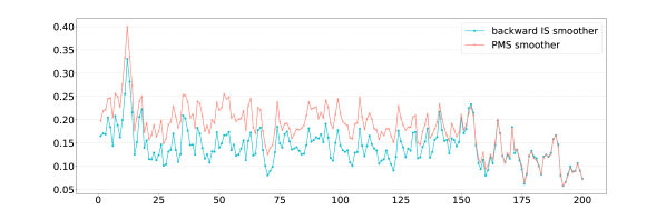
Figure 1: Plot of the empirical estimate of $\mathbb{E}[\|X_{k}-\mathbb{\widehat{E}}[X_{k}|Y_{0:199}]\|^{2}]$ for $k\in\{0,...,199\}$ for 100 runs of the Backward IS and Poor Man smoothers.

5.2 One dimensional diffusion processe: the Sine model

This section investigates the performance of the proposed algorithm to compute expectations under the smoothing distributions in a context where alternatives are available for comparison. Consider the Sine model where $(X_{t})_{t\geqslant 0}$ is assumed to be a weak solution to

$$\mathrm{d}X_{t}=\sin(X_{t}-\theta)\mathrm{d}t+\mathrm{d}W_{t}\;,\quad X_{0}=x_{0}\;.$$

This simple model has no explicit transition density, however, a General Poisson estimator which satisfies (12) can be computed by simulating Brownian bridges, (see [Beskos et al., 2006b]). Therefore, the backward importance sampling technique proposed in this paper can be compared to the usual acceptance-rejection algorithm described in Section 3.3. For this simple comparison, observations are received at evenly spaced times $t_{0}=0,\ldots,t_{10}=5$ from the model

$$Y_{k}=X_{t_{k}}+\varepsilon_{k},\;0\leqslant k\leqslant n=10\;,$$ (15)

where $(\varepsilon_{k})_{0\leqslant k\leqslant 10}$ are i.i.d. Gaussian random variables with mean $0$ and variance $1$. In this experiment $\theta=\pi/4$. The proposal distribution $p_{k}$ for the particle filtering approximation is chosen as the following approximation of the optimal filter:

$$p_{k}(x_{k},x_{k+1})\!\propto\!q^{\mathsf{Eul}}_{k+1}(x_{k},x_{k+1})g_{k+1}(x_{k+1},Y_{k+1})\;,$$ (16)

where $q^{\mathsf{Eul}}_{k+1}$ is the probability density function of Gaussian distibution with mean $\Delta\sin(x_{k}-\theta)$ and variance $\Delta$ where $\Delta=1/2$, i.e. the Euler approximation of the Sine SDE, and $g_{k}$ is the probability density function of the law of $Y_{k}$ given $X_{t_{k}}$ i.e. of a Gaussian random variable with mean $X_{t_{k}}$ and variance 1. As the observation model is linear and Gaussian, the proposal distribution is therefore Gaussian with explicit mean and variance.

In this first experiment, particles are used to solve the state estimation problem for the first observation i.e. to compute an estimate of $\mathbb{E}[X_{0}|Y_{0:n}]$. Figure 2 displays the computational complexity and the estimation of the posterior mean with the acceptance-rejection algorithm and the proposed backward sampling technique as a function of ${\widetilde{N}}$. In this setting, $N=100$, and each unbiased estimate of $\hat{q}$ is computed using 30 Monte Carlo replicates.

For ${\widetilde{N}}=2$ (which is the recommended value for the PaRIS algorithm, see [Olsson et al., 2017]), our estimate shows a bias, which is no surprise, as it is based on a biased normalized importance sampling step. However, this bias quickly vanishes for ${\widetilde{N}}\geqslant 10$. Interestingly, our method comes with a drastic (a factor 10) reduction of computational time. The vanishing of the bias might induce more backward sampling, but this remains much faster than the acceptance rejection method with ${\widetilde{N}}=2$.

Then, the same estimation was performed (on the same data set) for $N$ varying from 50 to 2000. In this context, ${\widetilde{N}}$ was set to 2 for the AR method. To have an empirical intuition of how ${\widetilde{N}}$ must vary with $N$ for our algorithm, the backward importance sampling is applied with ${\widetilde{N}}=N^{0.5},N^{0.6}$ and $N/10$ (as this last value was sufficient in the first experiment to avoid any bias). The results are shown in Figure 3. A small bias might appear for $N=2000$ and ${\widetilde{N}}\leavevmode\nobreak\ =\leavevmode\nobreak\ 45\;(\approx 2000^{0.5})$, but no bias is visible for $N^{0.6}$ and $N/10$. As expected, the gain in time, compared to the state of the art algorithm, remains important (even if it decreases as ${\widetilde{N}}$ increases). It is worth noting that the variance of the computational time is greatly reduced compared to the AR technique.

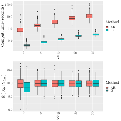
Figure 2: Computational complexity and estimation of a posterior mean as a function of the number of backward samples. Results are shown for the state of the art acceptance-rejection algorithm and the proposed backward importance sampling technique.

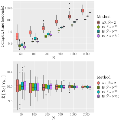
Figure 3: Computational complexity and estimation of a posterior mean as a function of the number of particles. Results are shown for the state of the art acceptance-rejection algorithm and the proposed backward importance sampling technique. The number of backward samples is set to 2 for the AR, and $N/10$ for the IS.

5.3 Recursive maximum likelihood estimation in the Sine model

Online recursive maximum likelihood using pseudo marginal SMC is illustrated for the same Sine model. As mentionned, a GPE estimator of the transition density can be computed. Following the idea of this computation, it is possible to obtain an unbiased estimate of the gradient of the log-transition density and thus compute and unbiased estimate of the key quantity given in (7). To the best of our knowledge, this estimator is new, and given in appendix A. Using the Exact algorithm of [Beskos et al., 2006a] a data set of 5000 points (displayed in Figure 4), was simulated whith the true parameter $\theta_{*}=\pi/4$. As in the previous section, particle smoothing was performed, using the same particle filter, with $N=100$ particles and ${\widetilde{N}}=10$ backward samples in our backward importance sampling procedure. In this setup, we explore three key features of our estimator.

Sensitivity to the starting point $\hat{\theta}_{0}$. The inference procedure was performed on the same data set from 50 different starting points uniformly chosen in $(0,2\pi)$. The gradient step size $\gamma_{k}$ of equation (9) was chosen constant (and equal to 0.5) for the first 300 time steps, and then decreasing with a rate proportional to $k^{-0.6}$. Results are given Figure 5. There is no sensitivity to the starting point of the algorithm, and after a couple of hundred observations, the estimates all concentrate around the true value. As the gradient step size decreases, the estimates stay around the true value following autocorrelated patterns that are common to all trajectories.

Asymptotic normality. The inference procedure was performed on 50 different data sets simulated with the same $\theta_{*}$. The 50 estimates were obtained starting from the same starting point (fixed to $\theta_{*}$, as Figure 5 shows no sensitivity to the starting point). Figure 6 shows the results for the raw and the averaged estimates. The averaged estimates $(\widetilde{\theta}_{k})_{k\geqslant 0}$ consist in averaging the values produced by the estimation procedure after a burning phase of $n_{0}$ time steps (here $n_{0}=300$ time steps). This procedure allows to obtain an estimator whose convergence rate does not depend on the step sizes chosen by the user, see [Polyak and Juditsky, 1992, Kushner and Yin, 1997]. For all $0\leqslant k\leqslant n_{0}$, $\widetilde{\theta}_{k}=\widehat{\theta}_{k}$ and for all $k>n_{0}$,

$$\widetilde{\theta}_{k}=\frac{1}{k-n_{0}}\sum_{j=n_{0}+1}^{k}\widehat{\theta}_{j}\;.$$

The estimated distribution of the final estimates seems to be Gaussian, centered around the true value. This conjecture, which would extend the asymptotic normality obtained in [Gloaguen et al., 2021] for the original pseudo-marginal PaRIS, should be proven in future works.

Step size influence. To illustrate the influence of the gradient step sizes, different settings are considered. In each scenario, the sequence $(\gamma_{k})_{k\geqslant 0}$ is given by

$$\gamma_{k}=\gamma_{0}\mathds{1}_{\left\{k\leq n_{0}\right\}}+\frac{\gamma_{0}}{(k-n_{0})^{\kappa}}\mathds{1}_{\left\{k>n_{0}\right\}}\;,$$

where $\gamma_{0}=0.5$. In this experiment $\kappa\in\{0.5,0.6,0.7,0.8,0.9,1\}$. The results are shown in Figure 7. As expected, the raw estimator shows different rates of convergence depending on $\kappa$, whereas the averaged estimator has the same behavior in all cases.

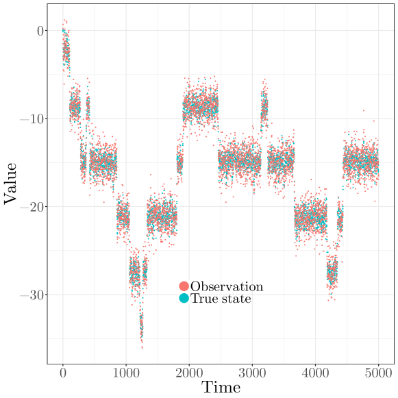
Figure 4: Data set simulated according to the SINE process, observed with noise at discrete time steps.

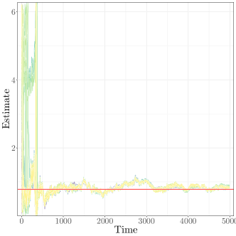
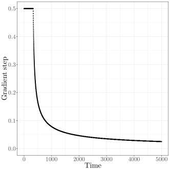
Figure 5: (Left) online estimation of $\theta$ for the data set presented in Figure 4. The algorithm is performed from 50 starting points. (Right) The gradient step sizes (defined in equation (9)).

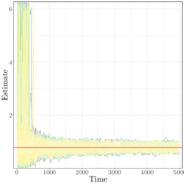
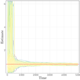
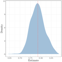
Figure 6: (Left) online estimation of $\theta$ for 50 different simulated data sets as presented in Figure 4. The algorithm is performed from 1 starting point with the gradient step size shown in Figure 5. (Center) Averaged estimator, where $\hat{\theta}$ is averaged after a burning phase of 300 time steps. (Right) Empirical distribution of $\hat{\theta}$. The red line is the value of $\theta^{*}$.

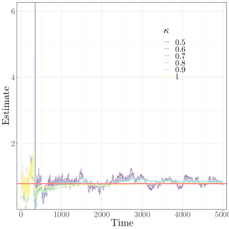
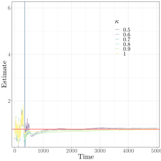
Figure 7: (Left) online estimation of $\theta$ for the data set presented in Figure 4, with different decreasing rates values $\kappa$. (Right) Averaged estimator, where $\hat{\theta}$ is averaged after a burning phase of 300 time steps.

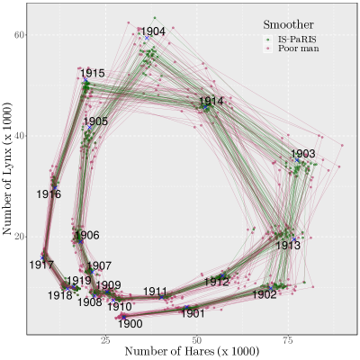
Figure 8: Estimated Hares-Lynx abundances using the Hudson bay company data set. Both our IS-PaRIS smoother and the poor man smoother are performed to approximate the MLE and solve the tracking problem. Blue crosses show the observations.

5.4 Multidimensional diffusion processes: Stochastic Lotka-Volterra model

This section sets the focus on a stochastic model describing in continuous time the population dynamics in a predator-prey system, as fully discussed in [Hening and Nguyen, 2018]. The bivariate process $(X_{t})_{t\geqslant 0}$ of predators and preys abundances is assumed to follow the stochastic Lotka-Volterra model:

$$\mathrm{d}X_{t}=\alpha_{\theta}(X_{t})\mathrm{d}t+\begin{pmatrix}X_{1}(t)&0\\ 0&X_{2}(t)\end{pmatrix}\Gamma\mathrm{d}\mathbf{W}_{t}\;,\$$ (17)

where $\mathbf{W}_{t}$ is a vector of independent standard Wiener processes, $\Gamma$ a $2\times 2$ matrix, and for $x=(x_{1},x_{2})^{T}:$

$$\alpha_{\theta}(x)=\begin{pmatrix}x_{1}(a_{10}-a_{11}x_{1}-a_{12}x_{2})\\ x_{2}(-a_{20}+a_{21}x_{1}-a_{22}x_{2})\end{pmatrix}\;.$$

In this context, the unknow parameter to be estimated is $\theta=(a_{10},a_{11},a_{12},a_{20},a_{21},a_{22},\Gamma)$. The observation model follows a widespread framework in ecology where the abundance of preys and predators are observed through some abundance index at discrete times $t_{0},\dots,t_{n}$:

$$Y_{t_{k}}=\begin{pmatrix}\text{c}_{1}X_{1}(t_{k})\mathrm{e}^{\epsilon^{(1)}_{t_{k}}}\\ \text{c}_{2}X_{2}(t_{k})\mathrm{e}^{\epsilon^{(2)}_{t_{k}}}\end{pmatrix}\;,$$ (18)

where $\text{c}=(\text{c}_{1},\text{c}_{2})^{T}$ is known (the observed fraction of the population) and $\{\epsilon_{t_{k}}=(\epsilon^{(1)}_{t_{k}},\epsilon^{(2)}_{t_{k}})\}_{1\leqslant k\leqslant n}$ are i.i.d. random variables distributed as a $\mathcal{N}_{2}(-\text{diag}\ \Sigma/2,\Sigma)$ where $\Sigma$ is an unknown 2 $\times$ 2 covariance matrix. It is straightforward to show that for a generic $\theta$, in the SDE defined by (17), the drift function cannot be written (even after the Lamperti transform) as the gradient of a potential. Therefore, the General Poisson estimator cannot be used as an unbiased estimator of the transition density. Following Section 4.1, an almost surely positive unbiased estimate of the transition density is obtained by combining the Wald’s trick to the parametrix estimators of [Fearnhead et al., 2017]. The proposal distribution for the particle filter is again a trade off between model dynamics and the observation model (full details are given in the appendix). The simulated set of particles is used to obtain estimates of the true abundances given the observations, both on synthetic and real data.

Synthetic data

In a first approach, simulated data are obtained from the model given by (17) and (18) for a known set of parameters. Chosen values of $\theta$, $\Sigma$, $\text{c}_{1}$ and $\text{c}_{2}$ for the experiment are given in the appendix. The model is used to simulate abundances indexes $Y_{0},\dots Y_{300}$ at times $t_{0}=0,\dots,t_{300}=3$. The associated time series (after a division by the known constant c) is shown in Figure 9 (left panel). In this experiment, the goal is to obtain an estimate of the actual predator-prey abundances given all the observed abundances indexes $Y_{0:n}$. Our estimate is given by the set of conditional expectations $\{\mathbb{E}[X_{k}|Y_{0:n}]\}_{k=0,\dots,n}$, approximated using our backward importance sampling PaRIS smoother, which is run using the true parameters. Figure 9 shows the estimated abundance trajectory over time. The proposed backward importance sampling smoother manages to estimate efficiently the actual abundance from noisy data and a model with an intractable transition density.

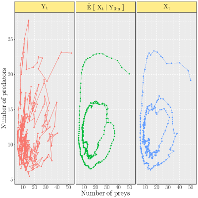
Figure 9: Estimated predator-prey abundances (center) in a stochastic Lotka Volterra model using our backward sampling estimate on simulated abundance indexes (left). Right panel shows the ground truth.

Hares and lynx data

In this section, the model defined by equations (17) and (18) is applied to the Hudson Bay company data, giving the number of hares and lynx trapped in Canada during the first 20 years of the 20th century (available in [Odum and Barrett, 1971]). As parameters are unknown in this case, maximum likelihood inference is performed using an EM [Dempster et al., 1977] algorithm to obtain an estimate $\hat{\theta}$. The E step is performed using the BIS smoother. At each iteration, the estimator $\theta_{k}$ is updated by finding a parameter $\theta_{k+1}$ for which $\hat{Q}(\theta_{k+1},\theta_{k})>\hat{Q}(\theta_{k},\theta_{k})$, with a gradient free evolution strategy [Hansen, 2006]. The last estimate $\hat{\theta}$ obtained with this EM algorithm is used to estimate the actual abundances in the model (similarly to the synthetic data case). Figure 8 shows estimates of $\mathbb{E}_{\hat{\theta}}\left[X_{k}|Y_{0:n}\right]$ obtained with 30 independent runs of our algorithm. The particle smoother is implemented using $N=200$ particles and $\tilde{N}=20$. The replicates show that the variance of our estimator (for a given set of observations) is much smaller than the one of the Poor Man’s smoother.

Appendix A Application to partially observed SDE

Let $(X_{t})_{t\geq 0}$ be defined as a weak solution to the following Stochastic Differential Equation (SDE) in $\mathbb{R}^{d}$:

$$X_{0}=x_{0}\quad\mbox{and}\quad\mathrm{d}X_{t}=\alpha_{\theta}(X_{t})\mathrm{d}t+\mathrm{d}W_{t}\;,$$ (19)

where $(W_{t})_{t\geqslant 0}$ is a standard Brownian motion, $\alpha_{\theta}:\mathbb{R}^{d}\to\mathbb{R}^{d}$ is the drift function . The inference procedure presented in this paper is applied in the case where the solution to (19) is supposed to be partially observed at times $t_{0}=0,\ldots,t_{n}$, for a given $n\geqslant 1$, through an observation process $(Y_{k})_{0\leqslant k\leqslant n}$ taking values in $\mathbb{R}^{m}$. For all $0\leqslant k\leqslant n$, the distribution of $Y_{k}$ given $(X_{t})_{t\geqslant 0}$ depends on $X_{k}=X_{t_{k}}$ only and has density $g_{k;\theta}$ with respect to $\nu$. The distribution of $X_{0}$ has density $\chi$ with respect to $\mu$ and for all $0\leqslant k\leqslant n-1$, the conditional distribution of $X_{k+1}$ given $(X_{t})_{0\leqslant t\leqslant k}$ has density $q_{k+1;\theta}(X_{k},\cdot)$ with respect to $\mu$.

A.1 Unbiased estimators of the transition densities

The algorithm described above strongly relies on assumption HH1. In the context of SDEs, when $g_{k+1;\theta}$ is available explicitly, this boils down to finding an unbiased estimate $\widehat{q}_{k+1;\theta}\langle\zeta\rangle(x,y)$ of $q_{k+1;\theta}(x,y)$ and defining

$$\mathsf{\ell}_{k;\theta}\langle\zeta\rangle(x,y)=\widehat{q}_{k+1;\theta}\langle\zeta\rangle(x,y)g_{k+1;\theta}(x_{k+1},Y_{k+1})\;.$$

A.2 General Poisson Estimators

In [Olsson et al., 2011] and [Gloaguen et al., 2018], General Poisson Estimators (GPEs) are used to obtain an unbiased estimate of the transition density. However, designing such estimators requires three strong assumptions [Beskos et al., 2006a].

1. The diffusion defined by (19) can be transformed into a unit diffusion through the Lamperti transform, with drift function $\tilde{\alpha}_{\theta}(x)$.

2. The drift of this unit diffusion can be expressed as the gradient of a potential function, i.e., there exists a twice differentiable function $A_{\theta}:\mathbb{R}^{d}\to\mathbb{R}$ such $\tilde{\alpha}_{\theta}=\nabla_{x}A_{\theta}$.

3. The function $x\mapsto(\|\tilde{\alpha}_{\theta}(x)\|^{2}+\Delta A_{\theta}(x))/2$ (where $\Delta$ denotes the Laplacian) is lower bounded.

Assumption (1) is used to define a proposal distribution absolutely continuous with respect to the target which is easy to sample from. Assumption (2) is necessary to obtain a tractable Radon-Nikodym derivative between the proposal and the target distributions using the Girsanov transformation. While these assumptions can be proved under mild assumptions for scalar diffusions, much stronger conditions are required in the multidimensional case [Aït-Shalia, 2008].

Let $\omega=(\omega_{s})_{0\leq s\leq t}$ be the realization of a Brownian Bridge starting at $x$ at time 0 and ending in $y$ at time $\Delta$. The distribution of $\omega$ is denoted by $\mathbb{W}_{x}^{\Delta,y}$. Moreover, suppose that for all $\theta\in\Theta$, $\alpha_{\theta}$ is of a gradient form $\alpha_{\theta}=\nabla_{x}A_{\theta}$ where $A_{\theta}:\mathbb{R}^{d}\to\mathbb{R}$ is a twice continuously differentiable function. Denoting, $\psi_{\theta}:\leavevmode\nobreak\ \leavevmode\nobreak\ x\mapsto\psi_{\theta}(x)=(\|\alpha_{\theta}(x)\|^{2}+\Delta A_{\theta}(x))/2$, by Girsanov theorem, for all $x,y\in\mathbb{R}^{d}\times\mathbb{R}^{d}$

$$q_{k+1;\theta}(x,y)=\phi_{\Delta_{k}}(x-y)\mathrm{exp}\left(A_{\theta}(y)-A_{\theta}(x)\right)\mathbb{E}_{\mathbb{W}_{x}^{\Delta_{k},y}}\left[\mathrm{exp}\left(-\int_{0}^{\Delta_{k}}\psi_{\theta}(\omega_{s})\mathrm{d}s\right)\right]\;,$$ (20)

where $\Delta_{k}=t_{k+1}-t_{k}$, for all $a>0$, $\phi_{a}$ is the probability density function of a centered Gaussian random variable with variance $a$. The transition density then cannot be computed as it involves an integration over the whole path between $x$ and $y$. To perform the algorithm proposed in this paper, we therefore have to design a positive an unbiased estimator of $q_{k+1;\theta}(x,y)$.

Unbiased GPE estimator for $q_{k+1;\theta}(x,y;\zeta)$.

Assume that there exist random variables $\underline{m}_{\theta}$ and $\overline{m}_{\theta}$ such that for all $0\leqslant s\leqslant\Delta_{k}$, $\underline{m}_{\theta}\leqslant\psi_{\theta}(\omega_{s})\leqslant\overline{m}_{\theta}$. Let $\kappa$ be a random variable taking values in $\mathbb{N}$ with distribution $\mu$, $\omega=(\omega_{s})_{0\leq s\leq\Delta_{k}}$ be the realization of a Brownian Bridge, and $(U_{j})_{1\leqslant j\leqslant\kappa}$ be independent uniform random variables on $(0,\Delta_{k})$ and $\zeta=(\kappa,\omega,U_{1},\ldots,U_{\kappa})$. As shown in [Fearnhead et al., 2008], equation (20) leads to a positive unbiased estimator given by

$$\widehat{q}_{k+1;\theta}(x,y;\zeta)=\phi_{\Delta_{k}}(x-y)\mathrm{exp}\left(A_{\theta}(y)-A_{\theta}(x)-\underline{m}_{\theta}\Delta_{k}\right)\prod_{j=1}^{\kappa}\frac{\overline{m}_{\theta}-\psi_{\theta}(\omega_{{U_{j}}})}{\overline{m}_{\theta}-\underline{m}_{\theta}}\;.$$

Unbiased GPE estimator of $\nabla_{\theta}\log q_{k+1;\theta}(x,y)$.

Let’s denote $\varphi_{\theta}:\leavevmode\nobreak\ x\mapsto\psi_{\theta}(x)-\underline{m}_{\theta}$. By (20),

$$\nabla_{\theta}\log q_{k+1;\theta}(x,y)=\nabla_{\theta}A_{\theta}(y)-\nabla_{\theta}A_{\theta}(x)-\nabla_{\theta}\underline{m}_{\theta}\Delta_{k}\\ -\frac{\mathbb{E}_{\mathbb{W}_{x}^{\Delta_{k},y}}\left[\left(\int_{0}^{\Delta_{k}}\nabla_{\theta}\varphi_{\theta}(\omega_{s})\mathrm{d}s\right)\mathrm{exp}\left(-\int_{0}^{\Delta_{k}}\varphi_{\theta}(\omega_{s})\mathrm{d}s\right)\right]}{\mathbb{E}_{\mathbb{W}_{x}^{\Delta_{k},y}}\left[\mathrm{exp}\left(-\int_{0}^{\Delta_{k}}\varphi_{\theta}(\omega_{s})\mathrm{d}s\right)\right]}\;.$$

On the other hand, the diffusion bridge $\mathbb{S}^{\Delta_{k},y}_{\theta,x}$ associated with the SDE (19) is absolutely continuous with respect to $\mathbb{W}_{x}^{\Delta_{k},y}$ with Radon-Nikodym derivative given by

$$\frac{\mathrm{d}\mathbb{S}^{\Delta_{k},y}_{\theta,x}}{\mathrm{d}\mathbb{W}_{x}^{\Delta_{k},y}}(\omega) =\left[q_{k+1;\theta}(x,y)\right]^{-1}\phi_{\Delta_{k}}(x-y)\mathrm{exp}\left(A_{\theta}(y)-A_{\theta}(x)-\underline{m}_{\theta}\Delta_{k}-\int_{0}^{\Delta_{k}}\varphi_{\theta}(\omega_{s})\mathrm{d}s\right)\;,$$

$$=\mathbb{E}_{\mathbb{W}_{x}^{\Delta_{k},y}}\left[\mathrm{exp}\left(-\int_{0}^{\Delta_{k}}\varphi_{\theta}(\omega_{s})\mathrm{d}s\right)\right]^{-1}\mathrm{exp}\left(-\int_{0}^{\Delta_{k}}\varphi_{\theta}(\omega_{s})\mathrm{d}s\right)\;.$$

This yields

$$\nabla_{\theta}\log q_{k+1;\theta}(x,y)=\left(\nabla_{\theta}A_{\theta}(y)-\nabla_{\theta}A_{\theta}(x)-\nabla_{\theta}\underline{m}_{\theta}\Delta_{k}\right)-\mathbb{E}_{\mathbb{S}_{\theta,x}^{\Delta_{k},y}}\left[\int_{0}^{\Delta_{k}}\nabla_{\theta}\varphi_{\theta}(\omega_{s})\mathrm{d}s\right]$$

and an unbiased estimator of $\nabla_{\theta}\log q_{k+1;\theta}(x,y)$ is given by

$$\mathsf{l}_{k+1;\theta}(x,y,\mathsf{s}^{\theta,x,y,\Delta_{k}}_{U})=\left(\nabla_{\theta}A_{\theta}(y)-\nabla_{\theta}A_{\theta}(x)-\nabla_{\theta}\underline{m}_{\theta}\Delta_{k}\right)-\Delta_{k}\nabla_{\theta}\varphi_{\theta}(\mathsf{s}^{\theta,x,y,\Delta_{k}}_{U})\;,$$

where $U$ is uniform on $(0,1)$ and independent of $\mathsf{s}^{\theta,x,y,\Delta_{k}}\sim\mathbb{S}_{\theta,x}^{\Delta_{k},y}$. In the context of GPE, $\mathsf{s}^{\theta,x,y,\Delta_{k}}$ can be simulated exactly using exact algorithms for diffusion processes proposed in [Beskos et al., 2006a].

A.3 Parametrix estimators

More recently, [Andersson and Kohatsu-Higa, 2017] and [Fearnhead et al., 2017] proposed an algorithm which can be used under weaker assumptions. This parametrix algorithm draws weighted skeletons using an importance sampling mechanism for diffusion processes. In this case, the sampled paths are not distributed as the target process but the weighted samples produce unbiased estimates of expectations of functionals of this process. To obtain an unbiased estimator $\widehat{q}_{k+1}\langle\zeta\rangle(x,y)$, the parametrix algorithm draws weighted skeletons at random times $s_{0}=0<s_{1}<\dots<s_{j}$, denoted by $\left\{(x_{s_{j}},\mathsf{w}_{s_{j}})\right\}_{j\geqslant 0}$, where $x_{0}=x$ and $\mathsf{w}_{0}=1$. The update times $(s_{j})_{j\geqslant 0}$ are instances of an inhomogeneous Poisson process of intensity $\lambda(t)$. Let $(x_{s_{j}},\mathsf{w}_{s_{j}})$ be the last weighted sample and $s_{j+1}$ be the next update time of the trajectory. While $s_{j+1}<\Delta t_{k}$, the new state is sampled using a simple Euler scheme, namely:

$$x_{s_{j+1}} :=x_{s_{j}}+\Delta s_{j}\alpha_{\theta}(x_{s_{j}})+(\Delta s_{j})^{1/2}\sigma_{\theta}(x_{s_{j}})\varepsilon_{j+1}\;,$$

where $\Delta s_{j}:=s_{j+1}-s_{j}$, $\Delta t_{k}=t_{k+1}-t_{k}$ and $\varepsilon_{j+1}\sim\mathcal{N}_{d}(0,I_{d})$. The proposal density associated with this procedure is denoted by $m_{j;\theta}\left(x_{s_{j}},\cdot,\Delta\tau_{j}\right)$. Let $\mathcal{K}^{\theta}$ (resp. $\mathcal{K}^{j,\theta}_{\mathrm{prop}}$) denote the Kolmogorov forward operator of the diffusion (resp. the Kolmogorov forward operator of the proposal distribution $m_{j;\theta}\left(x_{s_{j}},\cdot,\Delta s_{j}\right)$). The forward operators write, for any function $h:\mathbb{R}^{d}\rightarrow\mathbb{R}$,

$$\mathcal{K}^{\theta}h\left(y\right):=-\sum_{i=1}^{d}\frac{\partial}{\partial y_{i}}\left\{\alpha_{\theta,i}(y)h\left(y\right)\right\}+\sum_{i,\ell=1}^{d}\frac{1}{2}\frac{\partial^{2}}{\partial y_{i}\partial y_{\ell}}\left\{\gamma_{\theta,i,\ell}(y)h\left(y\right)\right\}\;,$$

where $\gamma_{\theta}=\sigma_{\theta}\sigma_{\theta}^{T}$. Then, following [Fearnhead et al., 2017], the weight is updated by

$$\mathsf{w}_{s_{j+1}}:=\mathsf{w}_{s_{j}}\rho^{\lambda}_{j}\left(x_{s_{j}},x_{s_{j+1}},\Delta s_{j}\right)\;,$$

where

$$\rho^{\lambda}_{j}\left(x,y,u\right):=1+\frac{\left(\mathcal{K}-\mathcal{K}^{j,\theta}_{\mathrm{prop}}\right)m_{j;\theta}\left(x,z,u\right)_{|z=y}}{\lambda(u)m_{j;\theta}\left(x,y,u\right)}\;.$$ (21)

It is worth noting that (21) can be computed using only first derivatives of $\alpha_{\theta}$ and second derivatives of $\sigma_{\theta}$. If $N_{k}$ is the number of Poisson events between $0$ and $\Delta t_{k}$, the parametrix unbiased estimate is then given by

$$\widehat{q}_{k+1}\langle\zeta_{k}\rangle(x,y)=\mathsf{w}_{s_{N_{k}}}m_{k;\theta}\left(x_{s_{N_{k}}},y,t_{k+1}-s_{N_{k}}\right)\;,$$

where $\zeta_{k}$ stands for all the randomness required to produce the parametrix estimator (Poisson process and Gaussian random variables).

The stability of this estimator is studied in [Fearnhead et al., 2017] which provides $\mathrm{L}_{p}$ controls for the weight $\mathsf{w}_{s_{N_{k}}}$. The parametrix algorithm mentioned above is a highly flexible procedure to obtain such an unbiased estimate for a much broader class of diffusions than Poisson based estimations which require strong assumptions. However, as the update (21) involves the difference of two Kolmogorov operators, the parametrix estimator of the transition density may be negative, and has no reason to satisfy (12).

References

- [Aït-Shalia, 2008] Aït-Shalia, Y. (2008). Closed-form likelihood expansions for multivariate diffusions. Annals of Statistics, 36(2):906–937.
- [Andersson and Kohatsu-Higa, 2017] Andersson, P. and Kohatsu-Higa, A. (2017). Unbiased simulation of stochastic differential equations using parametrix expansions. Bernoulli, 23(3):2028–2057.
- [Andrieu and Roberts, 2009] Andrieu, C. and Roberts, G. O. (2009). The pseudo-marginal approach for efficient Monte Carlo computations. The Annals of Statistics, 37(2):697 – 725.
- [Beskos et al., 2006a] Beskos, A., Papaspiliopoulos, O., and Roberts, G. O. (2006a). Retrospective exact simulation of diffusion sample paths with applications. Bernoulli, 12(6):1077–1098.
- [Beskos et al., 2006b] Beskos, A., Papaspiliopoulos, O., Roberts, G. O., and Fearnhead, P. (2006b). Exact and computationally efficient likelihood-based estimation for discretely observed diffusion processes (with discussion). Journal of the Royal Statistical Society: Series B (Statistical Methodology), 68(3):333–382.
- [Briers et al., 2010] Briers, M., Doucet, A., and Maskell, S. (2010). Smoothing algorithms for state–space models. Annals of the Institute of Statistical Mathematics, 62(1):61.
- [Candanedo et al., 2017] Candanedo, L. M., Feldheim, V., and Deramaix, D. (2017). A methodology based on hidden markov models for occupancy detection and a case study in a low energy residential building. Energy and Buildings, 148:327–341.
- [Cappé et al., 2005] Cappé, O., Moulines, E., and Rydén, T. (2005). Inference in Hidden Markov Models. Springer.
- [Cho et al., 2014] Cho, K., van Merriënboer, B., Gulcehre, C., Bougares, F., Schwenk, H., and Bengio, Y. (2014). Learning phrase representations using rnn encoder-decoder for statistical machine translation.
- [Del Moral et al., 2010] Del Moral, P., Doucet, A., and Singh, S. S. (2010). A backward particle interpretation of feynman-kac formulae. ESAIM: Mathematical Modelling and Numerical Analysis, 44(5):947–975.
- [Del Moral et al., 2015] Del Moral, P., Doucet, A., and Singh, S. S. (2015). Uniform stability of a particle approximation of the optimal filter derivative. SIAM Journal on Control and Optimization, 53(3):1278–1304.
- [Dempster et al., 1977] Dempster, A., Laird, N., and Rubin, D. (1977). Maximum likelihood from incomplete data via the EM algorithm (with discussion). 39:1–38.
- [Douc et al., 2011] Douc, R., Garivier, A., Moulines, E., and Olsson, J. (2011). Sequential monte carlo smoothing for general state space hidden markov models. The Annals of Applied Probability, 21(6):2109–2145.
- [Douc et al., 2014] Douc, R., Moulines, E., and Stoffer, D. (2014). Nonlinear time series: theory, methods and applications with R examples. CRC Press.
- [Dubarry and Le Corff, 2013] Dubarry, C. and Le Corff, S. (2013). Non-asymptotic deviation inequalities for smoothed additive functionals in nonlinear state-space models. Bernoulli, 19(5B):2222–2249.
- [Fearnhead et al., 2017] Fearnhead, P., Latuszynski, K., Roberts, G. O., and Sermaidis, G. (2017). Continuous-time importance sampling: Monte carlo methods which avoid time-discretisation error. arXiv preprint arXiv:1712.06201.
- [Fearnhead et al., 2010a] Fearnhead, P., Papaspiliopoulos, O., Roberts, G., and Stuart, A. (2010a). Random weight particle filtering of continuous time stochastic processes. Journal of the Royal Statistical Society: Series B (Statistical Methodology), 72(4):497–512.
- [Fearnhead et al., 2008] Fearnhead, P., Papaspiliopoulos, O., and Roberts, G. O. (2008). Particle filters for partially observed diffusions. Journal of the Royal Statistical Society: Series B (Statistical Methodology), 70(4):755–777.
- [Fearnhead et al., 2010b] Fearnhead, P., Wyncoll, D., and Tawn, J. (2010b). A sequential smoothing algorithm with linear computational cost. Biometrika, 97(2):447–464.
- [Gassiat et al., 2016] Gassiat, É., Cleynen, A., and Robin, S. (2016). Inference in finite state space non parametric hidden markov models and applications. Statistics and Computing, 26(1-2):61–71.
- [Gerber and Chopin, 2017] Gerber, M. and Chopin, N. (2017). Convergence of sequential quasi-Monte Carlo smoothing algorithms. Bernoulli, 23(4B):2951–2987.
- [Gloaguen et al., 2018] Gloaguen, P., Etienne, M.-P., and Le Corff, S. (2018). Online sequential monte carlo smoother for partially observed diffusion processes. EURASIP Journal on Advances in Signal Processing, 2018(1):9.
- [Gloaguen et al., 2021] Gloaguen, P., Le Corff, S., and Olsson, J. (2021). A pseudo-marginal sequential Monte Carlo online smoothing algorithm. working paper or preprint.
- [Gordon et al., 1993] Gordon, N. J., Salmond, D. J., and Smith, A. F. (1993). Novel approach to nonlinear/non-gaussian bayesian state estimation. In IEE proceedings F (radar and signal processing), volume 140, pages 107–113. IET.
- [Hansen, 2006] Hansen, N. (2006). The cma evolution strategy: a comparing review. In Towards a new evolutionary computation, pages 75–102. Springer.
- [Hening and Nguyen, 2018] Hening, A. and Nguyen, D. H. (2018). Persistence in stochastic lotka–volterra food chains with intraspecific competition. Bulletin of mathematical biology, 80(10):2527–2560.
- [Hochreiter and Schmidhuber, 1997] Hochreiter, S. and Schmidhuber, J. (1997). Long short-term memory. Neural Computation, 9:1735–1780.
- [Kushner and Yin, 1997] Kushner, H. J. and Yin, G. G. (1997). Stochastic Approximation Algorithms and Applications. Springer.
- [Le Gland and Mevel, 1997] Le Gland, F. and Mevel, L. (1997). Recursive estimation in HMMs. In Proc. IEEE Conf. Decis. Control, pages 3468–3473.
- [Martin et al., 2014] Martin, J. S., Jasra, A., Singh, S. S., Whiteley, N., Del Moral, P., and McCoy, E. (2014). Approximate Bayesian Computation for smoothing. Stochastic Analysis and Applications, 32:397–420.
- [Michelot et al., 2016] Michelot, T., Langrock, R., and Patterson, T. A. (2016). movehmm: an r package for the statistical modelling of animal movement data using hidden markov models. Methods in Ecology and Evolution, 7(11):1308–1315.
- [Mikolov et al., 2010] Mikolov, T., Karafiát, M., Burget, L., Černockỳ, J., and Khudanpur, S. (2010). Recurrent neural network based language model. In Eleventh annual conference of the international speech communication association.
- [Mozer, 1989] Mozer, M. C. (1989). A focused backpropagation algorithm for temporal pattern recognition. Complex Systems, 3.
- [Nguyen et al., 2017] Nguyen, T., Le Corff, S., and Moulines, É. (2017). On the two-filter approximations of marginal smoothing distributions in general state-space models. Advances in Applied Probability, 50(1):154–177.
- [Odum and Barrett, 1971] Odum, E. P. and Barrett, G. W. (1971). Fundamentals of ecology, volume 3. Saunders Philadelphia.
- [Olsson and Alenlöv, 2020] Olsson, J. and Alenlöv, J. W. (2020). Particle-based online estimation of tangent filters with application to parameter estimation in nonlinear state-space models. Annals of the Institute of Statistical Mathematics, 72(2):545–576.
- [Olsson et al., 2011] Olsson, J., Ströjby, J., et al. (2011). Particle-based likelihood inference in partially observed diffusion processes using generalised poisson estimators. Electronic Journal of Statistics, 5:1090–1122.
- [Olsson et al., 2017] Olsson, J., Westerborn, J., et al. (2017). Efficient particle-based online smoothing in general hidden markov models: the paris algorithm. Bernoulli, 23(3):1951–1996.
- [Polyak and Juditsky, 1992] Polyak, B. T. and Juditsky, A. B. (1992). Acceleration of stochastic approximation by averaging. SIAM J. Control Optim., 30(4):838–855.
- [Rabiner, 1989] Rabiner, L. (1989). A tutorial on hidden markov models and selected applications in speech recognition. In Proceedings of the IEEE, pages 257–286.
- [Särkkä, 2013] Särkkä, S. (2013). Bayesian Filtering and Smoothing. Cambridge University Press, New York, NY, USA.
- [Särkkä et al., 2007] Särkkä, S., Vehtari, A., and Lampinen, J. (2007). Rao-Blackwellized particle filter for multiple target tracking. Inofrmation Fusion, 8(1):2–15.
- [Sutskever et al., 2011] Sutskever, I., Martens, J., and Hinton, G. E. (2011). Generating text with recurrent neural networks. In ICML.
- [Sutskever et al., 2014] Sutskever, I., Vinyals, O., and Le, Q. V. (2014). Sequence to sequence learning with neural networks. arXiv preprint arXiv:1409.3215.
- [Tadić, 2010] Tadić, V. (2010). Analyticity, convergence, and convergence rate of recursive maximum-likelihood estimation in hidden Markov models. IEEE Transactions on Information Theory, 56:6406–6432.
- [Wang et al., 2017] Wang, X., Lebarbier, E., Aubert, J., and Robin, S. (2017). Variational inference for coupled hidden markov models applied to the joint detection of copy number variations. The International Journal of Biostatistics, 15.
- [Yau et al., 2011] Yau, C., Papaspiliopoulos, O., Roberts, G. O., and Holmes, C. (2011). Bayesian non-parametric hidden Markov models with applications in genomics. 73:1–21.
- [Yonekura and Beskos, 2020] Yonekura, S. and Beskos, A. (2020). Online smoothing for diffusion processes observed with noise. ArXiv:2003.12247.
- [Zucchini et al., 2017] Zucchini, W., Mac Donald, I., and Langrock, R. (2017). Hidden Markov models for time series: an introduction using R. CRC Press.