Quenched and Annealed Disorder Mechanisms in Comb-Models with Fractional Operators

Abstract

Recent experimental findings on anomalous diffusion have demanded novel models that combine annealed (temporal) and quenched (spatial or static) disorder mechanisms. The comb-model is a simplified description of diffusion on percolation clusters, where the comb-like structure mimics quenched disorder mechanisms and yields a subdiffusive regime. Here we extend the comb-model to simultaneously account for quenched and annealed disorder mechanisms. To do so, we replace usual derivatives in the comb diffusion equation by different fractional time-derivative operators and the conventional comb-like structure by a generalized fractal structure. Our hybrid comb-models thus represent a diffusion where different comb-like structures describe different quenched disorder mechanisms, and the fractional operators account for various annealed disorders mechanisms. We find exact solutions for the diffusion propagator and mean square displacement in terms of different memory kernels used for defining the fractional operators. Among other findings, we show that these models describe crossovers from subdiffusion to Brownian or confined diffusions, situations emerging in empirical results. These results reveal the critical role of interactions between geometrical restrictions and memory effects on modeling anomalous diffusion.

I Introduction

The development of the diffusion concept has always relied on the mutually-beneficial relationship between theory and experiments. Since Perrin’s experiments proving Einstein’s diffusion theory Perrin (1910), Brownian (usual) diffusion is well-known to display a Gaussian distribution and a linear time dependence of the mean square displacement (MSD). However, as deviations from these usual behaviors started to appear in experimental studies of disordered media and biological systems, the need to understand underlying microscopic mechanisms of these unusual dynamics has given rise to breakthrough theories in statistical physics.

The anomalous diffusion era started with the concept of waiting-time distribution in random walks, proposed independently by Lévy Lévy (1954), Smith Smith (1955), and Montroll and Weiss Montroll and Weiss (1965); but the continuous-time random walk (CTRW) emerged as the foundation of anomalous transport only after the works of Scher and Lax Scher and Lax (1973a, b) on unusual results for charge transport in amorphous semiconductors. These works use CTRW to describe heterogeneities of a medium in an annealed way, where the waiting-time distribution represents the environment randomness. The “second youth” of the CTRW Kutner and Masoliver (2017) is usually marked by its relationship with fractional diffusion equations Klafter et al. (1987); Hilfer and Anton (1995); Compte (1996); Barkai (2002), a formalism that becomes known as an efficient phenomenological description of anomalous diffusion in complex systems Meztler and Klafter (2000); West (2016); Kutner and Masoliver (2017).

Percolation theory Broadbent and Hammersley (1957) represents another significant breakthrough for the description of anomalous diffusion. As emphasized by Havlin and Ben-Avraham Havlin and Ben-Avraham (2002), the percolation model is a simple and purely geometrical approach to describe disordered media. While random walk processes are generalized in the CTRW model, in percolation processes, usual random walks take place in a disordered environment. In contrast to the CTRW framework, percolation theory thus describes a quenched disorder, where the randomness associated with geometrical constraints are constant in time. Under this context, de Gennes de Gennes (1976) coined the term “the ant in a labyrinth” to describe random walks in percolation lattices and established a paradigm of anomalous diffusion caused by geometrical structures Bouchaud and Georges (1990); Bok et al. (2009). This paradigm becomes well established mainly due to fractal geometry Mandelbrot and Blumen (1989), and it is essential in the study of porous media Havlin and Ben-Avraham (2002).

Diffusion also becomes an essential noninvasive tool to probe and characterize systems ranging from materials to living organisms Sen (2004); Waigh (2005); Kirstein et al. (2007); Wirtz (2009); Novikov et al. (2014); Papaioannou et al. (2017); Assaf et al. (2019); Song et al. (2019). These recent empirical results revealed a myriad of complex patterns that are usually not well described by analytical tools developed for amorphous solids and porous media. As argued by Metzler Metzler (2017), these novel experimental findings require researchers to come up with novel models. In this context, hybrid or mixed models of anomalous diffusion emerged as a significant modeling possibility Meroz et al. (2010); Weigel et al. (2011); Jeon et al. (2011); Tabei et al. (2013); Miyaguchi and Akimoto (2015); Golan and Sherman (2017); Furnival et al. (2017). Examples include CTRW on fractals Meroz et al. (2010); Weigel et al. (2011); Golan and Sherman (2017), CTRW combined with fractal Brownian motion Jeon et al. (2011); Tabei et al. (2013), quenched-trap model and fractal lattices Miyaguchi and Akimoto (2015), and CTRW combined with percolation theory Furnival et al. (2017). In general, these models share the idea of combining annealed (temporal) and quenched (spatial or static) disorder mechanisms.

Another model of anomalous diffusion of particular importance to the present work is the comb-model; a model emerged from studies of percolation threshold and anomalous diffusion on fractal structures Coniglio (1981); Stanley and Coniglio (1984); White and Barma (1984); Havlin et al. (1987). This model describes a diffusive process on a comb-like structure consisting of a “backbone” (a single infinite line in the $x$-direction) and “branches” (parallel lines in the $y$-direction that intersect the $x$-axis). The comb-model is a simplified description of the fractal geometry of percolation clusters, where the backbone represents the large bond and branches are the remaining bonds or “dangling ends” of percolation clusters (Figures 1a and 1b). The comb-model retains essential properties of diffusion on fractals, with the advantage of providing exact results on such complicated systems. Moreover, random walks on comb-like structures established the sojourn times of walkers in the teeth as the underlying mechanism of anomalous diffusion in the backbone.

Figure 1: The comb-model as simplified description of diffusion on percolation cluster. (a) Illustration of a percolation cluster where the continuous lines indicate the large bond and dashed lines are the dangling ends. The comb-model shown in (b) and modeled by Eq. (1) is a simplified description of the geometry in percolation clusters. Panels (c) and (d) compare the usual two-dimensional diffusive process with the diffusion on comb structure. The two-dimensional diffusion imposes no geometrical restriction on random walkers, while horizontal shifts occur only when $y=0$ in the comb-model; to accesses different branches, walkers must return to the backbone. Subdiffusive behavior in the backbone is a direct consequence of branches acting like traps.

Given the previously-mentioned experimental findings and because the quenched disorder is intrinsic to the comb structure, it is essential to account for annealed disorder in the comb-model. Here we propose such hybrid comb-models by generalizing the usual comb diffusion equation Arkhincheev and Baskin (1991) via different fractional time-derivative operators. In our hybrid comb-models, different comb-like structures describe quenched disorder, and fractional operators account for annealed disorder. By exploring different configurations where fractional operators act on the branches, backbone, or simultaneously on both, and also by replacing the usual comb structure by a generalized fractal structure, we find a series of nontrivial results that are useful for describing some recent empirical results reported for anomalous diffusion. Among other findings, we observe that these generalized comb-models describe restricted diffusion, Brownian diffusion, and crossovers from subdiffusion to restricted or Brownian diffusions.

The rest of this manuscript is organized as follows. In Section II, we define our generalized version of the comb-model and investigate its solutions under different situations. In Section III, we consider a fractal grid in place the single backbone structure and explore the effects of this modification on the diffusive behavior. Finally, we conclude this work in Section IV with a discussion and summary of our findings.

II Generalized Comb-Models with Fractional Operators

The diffusion equation for a comb structure was proposed by Arkhincheev and Baskin Arkhincheev and Baskin (1991) and represents a two-dimensional Einstein’s diffusion equation where the diffusive term in the $x$-direction is multiplied by a Dirac delta function $\delta(y)$, that is,

$$\frac{\partial}{\partial t}\rho(x,y;t)={\cal{D}}_{y}\frac{\partial^{2}}{\partial y^{2}}\rho(x,y;t)+\delta(y){\cal{D}}_{x}\frac{\partial^{2}}{\partial x^{2}}\rho(x,y;t).$$ (1)

Because of the delta function, diffusion in the $x$-direction only occurs over the backbone structure (when $y=0$). The diffusion in the $y$-direction creates the branch structures; a walker can only leave a branch or access other branches by returning to the backbone structure (Figures 1c and 1d). The geometrical restrictions in Eq. (1) mimic all features of early comb-models, including subdiffusive behavior in the backbone. The trapping times over the branches are also equivalent to a power-law behavior in the waiting-time distributions of a CTRW. The solutions of Eq. (1) are related to a time-fractional diffusion equation (with an anomalous exponent $\alpha_{x}=1/2$) describing the spreading behavior in the backbone Arkhincheev and Baskin (1991); Arkhincheev (1999); El-Wakil et al. (2002); Iomin and Baskin (2005). The diffusion over the backbone is also described by a time-fractional diffusion equation with exponent $\alpha_{x}=1/4$ in a three-dimensional comb structure and $\alpha_{x}=1/2N$ for an $N$-dimensional case Arkhincheev (1999). Extensions of Eq. (1) have been used to obtain a fractional diffusion equation with an absorbent term and a linear external force Zahran (2009) as well as to deal with generalized fractal structures in the backbone and branches (namely the fractal comb-model) Iomin (2011); Sandev et al. (2015a, 2016a, 2017a).

In this context, we propose to generalize the comb-model by including different fractional time-derivative operators on the diffusion terms, that is,

$$\frac{\partial}{\partial t}\rho(x,y;t)={\cal{F}}_{t,y}\left({\cal{D}}_{y}\frac{\partial^{2}}{\partial y^{2}}\rho(x,y;t)\right)+\delta(y){\cal{F}}_{t,x}\left({\cal{D}}_{x}\frac{\partial^{2}}{\partial x^{2}}\rho(x,y;t)\right)\,,$$ (2)

where ${\cal{F}}_{t,i}\{\cdots\}$ is an operator defined by the time derivative of a convolution integral between a function $f(x,y,t)$ and a memory kernel $\mathcal{K}_{i}(t)$ ($i\in\{x,y\}$), that is,

$${\cal{F}}_{t,i}\{f(x,y;t)\}=\frac{\partial}{\partial t}\int_{0}^{t}f(x,y;t^{\prime})\mathcal{K}_{i}(t-t^{\prime})\,dt^{\prime}\;.$$ (3)

The use of fractional derivatives in front of spatial operators is motivated by a possible connection with the linear-response theory Sokolov (2001). The memory kernel can also be connected with the waiting-time distribution of CTRW and represents a coarse-grained description of the environment’s randomness. Specifically, the kernel of the time-convoluted operator represents a density memory (a property of a collection of trajectories) and not a trajectory memory Cakir et al. (2007). A derivation of this integro-differential operator and the physical meaning of the memory kernel are given by Sokolov and Klafter Sokolov and Klafter (2005). It is worth mentioning that different operators Sokolov (2002); Lenzi et al. (2010); Chechkin et al. (2002) have been used to extend diffusion equations. For instance, the operator $\int_{0}^{t}f(x,y;t^{\prime})\mathcal{K}_{i}(t-t^{\prime})\,dt^{\prime}$ was considered by Sokolov Sokolov (2002) for identifying memory kernels that lead non-negative solutions (safe ones) and those that this condition is not guaranteed (dangerous ones).

The memory kernels $\mathcal{K}_{i}(t)$ define the integro-differential operators in Eq. (2) and establish a connection with fractional time-derivative operators. Thus, Eq. (3) represents a unified description for a broad class of situations where either singular or non-singular kernels describe different relaxation processes. Moreover, distinct kernels for the $x$ and $y$ directions yield anisotropic diffusion. Equations (2) and (3) recover the usual comb-model [Eq. (1)] when $\mathcal{K}_{x}(t)=\mathcal{K}_{y}(t)=1$. In the usual case, there are no memory effects, and geometrical restrictions of the comb-like structure are the only mechanism tied to the anomalous diffusion Sandev et al. (2015a); Iomin et al. (2018).

Different choices for $\mathcal{K}_{x}(t)$ and $\mathcal{K}_{y}(t)$ imply in extending the comb-model to different contexts that combine quenched and annealed disorders. One possibility is to consider power-law functions such as

$$\mathcal{K}_{i}(t)=\frac{t^{\alpha_{i}-1}}{\Gamma\left(\alpha_{i}\right)},$$ (4)

which are directly related to the Riemann-Liouville fractional operator Podlubny (1999) for $0<\alpha_{i}<1$. This fractional operator has been used to investigate several physical contexts, in particular the ones related to anomalous diffusion Meztler and Klafter (2000); Barkai (2001); Evangelista and Lenzi (2018).

Another possibility is to assume an exponential behavior for the kernels

$$\mathcal{K}_{i}(t) = {\cal{R}}(\alpha^{\prime}_{i})\exp\left(-\alpha^{\prime}_{i}\,t\right)\,,$$ (5)

where ${\cal{R}}(\alpha^{\prime}_{i})$ is a normalization constant. This choice corresponds to the Caputo-Fabrizio operator with $\alpha^{\prime}_{i}=\alpha_{i}/(1-\alpha_{i})$ Caputo and Fabrizio (2015); Hristov (2017); Tateishi et al. (2017). A remarkable feature of this exponential kernel is its connection with resetting processes Tateishi et al. (2017). In particular, by combining Eqs. (2), (3), and (5), we find

$$\frac{\partial}{\partial t}\rho(x,y;t)={\cal{D}}_{y}\frac{\partial^{2}}{\partial y^{2}}\rho(x,y;t)+\delta(y){\cal{D}}_{x}\frac{\partial^{2}}{\partial x^{2}}\rho(x,y;t)-\tilde{\alpha}\left(\rho(x,y,t)-\varphi(x,y)\right)\,,$$ (6)

where $\alpha_{x}=\alpha_{y}=\tilde{\alpha}$ and $\varphi(x,y)$ is the initial condition. Equation (6) extends the standard expressions used to analyze resetting processes by including a geometric constraint between the $x$ and $y$ directions. It is worth noticing that an exponential kernel leads to the Cattaneo equation in the approach of Sokolov Sokolov (2002), that is, a diffusion-wave equation different from Eq. (6). The kernel ${\cal K}_{\alpha_{i}}(t)\propto\,E_{\alpha}\left(-\overline{\alpha}t^{\alpha}\right)$, where

$$E_{\alpha}(z)=\sum_{k=0}^{\infty}\frac{z^{k}}{\Gamma(\alpha k+1)}$$ (7)

is the Mittag-Leffler function Podlubny (1999) with parameter $\alpha$ and $\overline{\alpha}$ a constant, somehow interpolates between the power-law and exponential cases and has been recently associated with fractional-time derivatives of distributed order Tateishi et al. (2017). It is worth mentioning that these non-singular kernels have been used to investigate different contexts such as diffusion Tateishi et al. (2017), heat processes Basa et al. (2019), groundwater flow Atangana and Baleanu (2017), and electrical circuits Gomez-Aguilar et al. (2016).

We now focus on the solutions of Eq. (2) in the Fourier-Laplace domain by using the Green function approach. After, we analyze particular cases related to the previous kernels. We consider Eq. (2) subjected to the initial condition $\rho(x,y,0)=\varphi(x,y)$, where $\varphi(x,y)$ is a normalized function, that is, $\int_{-\infty}^{\infty}dx\int_{-\infty}^{\infty}dy\,\varphi(x,y)=1$. We further assume $\rho(\pm\infty,y;t)=0$ and $\rho(x,\pm\infty;t)=0$ as boundary conditions. These unlimited boundary conditions avoid possible effects of confinement in a limited domain, making more explicit the impact of geometrical restrictions and fractional operators on the spreading behavior.

To obtain the solutions of Eq. (2), we first apply the Laplace transform $\left({\mathcal{L}}\left\{\rho(x,y;t)\right\}\right.=$ $\left.\int_{0}^{\infty}e^{-st}\rho(x,y;t)\,dt=\bar{\rho}(x,y;s)\right)$, yielding

$$s\bar{\rho}(x,y;s)-\varphi(x,y)=s\bar{\mathcal{D}}_{y}(s)\frac{\partial^{2}}{\partial y^{2}}\bar{\rho}(x,y;s)+\delta(y)s\bar{{\cal{D}}}_{x}(s)\frac{\partial^{2}}{\partial x^{2}}\bar{\rho}(x,y;s),$$ (8)

where $\bar{\mathcal{D}}_{y}(s)={\cal{D}}_{y}\bar{\mathcal{K}}_{y}(s)$ and $\bar{\mathcal{D}}_{x}(s)={\cal{D}}_{x}\bar{\mathcal{K}}_{x}(s)$. We next apply the Fourier transform $\left({\mathcal{F}}\left\{\rho(x,y;t)\right\}=\tilde{\rho}(k_{x},y;s)=\right.$ $\left.\int_{-\infty}^{\infty}e^{-ik_{x}x}\rho(x,y;t)\,dx\right.)$ on the $x$ variable of Eq. (8), yielding

$$s\bar{{\cal{D}}}_{y}(s)\frac{d^{2}}{dy^{2}}\bar{\rho}(k_{x},y;s)-s\left(1-\delta(y)\bar{{\cal{D}}}_{x}(s)k_{x}^{2}\right)\bar{\rho}(k_{x},y;s)=-\varphi(k_{x},y)\;.$$ (9)

By using the Green functions approach, the solution for Eq. (9) is written as

$$\bar{\rho}(k_{x},y;s)=-\int_{-\infty}^{\infty}dy^{\prime}\,\varphi(k_{x},y^{\prime})\bar{{\cal{G}}}(k_{x},y,y^{\prime};s)\,,$$ (10)

where the Green function ${\cal{G}}(k_{x},y,y^{\prime};s)$ is the solution of

$$s\bar{{\cal{D}}}_{y}(s)\frac{d^{2}}{dy^{2}}\bar{{\cal{G}}}(k_{x},y,y^{\prime};s)-\left(s+\delta(y)s\bar{{\cal{D}}}_{x}(s)k_{x}^{2}\right)\bar{{\cal{G}}}(k_{x},y,y^{\prime};s)=\delta(y-y^{\prime})$$ (11)

subjected to the condition $\bar{{\cal{G}}}(k_{x},\pm\infty,\bar{y};s)=0$.

After some calculations, we can show that the solution for Eq. (11) is

$$\tilde{\bar{{\cal{G}}}}(k_{x},y,y^{\prime};s)=-\frac{1}{2s\sqrt{\bar{{\cal{D}}}_{y}(s)}}e^{-\frac{1}{\sqrt{\bar{{\cal{D}}}_{y}(s)}}|y-y^{\prime}|}-\frac{\bar{{\cal{D}}}_{x}(s)k_{x}^{2}}{2\sqrt{\bar{{\cal{D}}}_{y}(s)}}e^{-\frac{1}{\sqrt{\bar{{\cal{D}}}_{y}(s)}}|y|}\bar{{\cal{G}}}(k_{x},0,y^{\prime};s),$$ (12)

where

$$\!\!\!\!\!\!\tilde{\bar{{\cal{G}}}}(k_{x},0,y^{\prime};s)=\frac{e^{-\frac{1}{\sqrt{{\cal{D}}_{y}(s)}}|y^{\prime}|}}{s\left({\cal{D}}_{x}(s)k_{x}^{2}+2\sqrt{{\cal{D}}_{y}(s)}\right)}\;$$ (13)

represents the propagator for the backbone structure (at $y=0$). The term ${\cal{D}}_{y}(s)$ in Eq. (13) indicates that the backbone diffusion explicitly depends on the diffusion occurring along the branches; in other words, memory effects on branches directly affect the diffusion on the backbone.

The Green function related to Eq. (11) subjected to previous boundary condition is thus given by

$$\!\!\!\!\!\!\bar{{\cal{G}}}(k_{x},y,y^{\prime};s) = -\frac{1}{2s\sqrt{\bar{{\cal{D}}}_{y}(s)}}e^{-\frac{1}{\sqrt{\bar{{\cal{D}}}_{y}(s)}}|y-y^{\prime}|}+\frac{\bar{{\cal{D}}}_{x}(s)k_{x}^{2}}{\bar{{\cal{D}}}_{x}(s)k_{x}^{2}+2\sqrt{\bar{{\cal{D}}}_{y}(s)}}\frac{1}{2s\sqrt{\bar{{\cal{D}}}_{y}(s)}}e^{-\frac{1}{\sqrt{\bar{{\cal{D}}}_{y}(s)}}\left(|y|+|y^{\prime}|\right)}$$ (14)

$$= -\frac{1}{2s\sqrt{\bar{{\cal{D}}}_{y}(s)}}\left(e^{-\frac{1}{\sqrt{\bar{{\cal{D}}}_{y}(s)}}|y-y^{\prime}|}-e^{-\frac{1}{\sqrt{\bar{{\cal{D}}}_{y}(s)}}\left(|y|+|y^{\prime}|\right)}\right)$$

$$- \frac{1}{s\left(2\sqrt{\bar{{\cal{D}}}_{y}(s)}+\bar{{\cal{D}}}_{x}(s)k_{x}^{2}\right)}e^{-\frac{1}{\sqrt{\bar{{\cal{D}}}_{y}(s)}}\left(|y|+|y^{\prime}|\right)}\;.$$

After performing the inverse Fourier transform on $x$-direction $({\mathcal{F}}^{-1}\left\{\tilde{\rho}(k_{x},y;t)\right\}$ $=$ $\rho(x,y;t)$ $=$ $\int_{-\infty}^{\infty}e^{ik_{x}x}\tilde{\rho}(k_{x},y;t)\,dk_{x})$, we obtain

$${\cal{G}}(x,y,y^{\prime};s) = -\frac{\delta(x)}{2s\sqrt{\bar{{\cal{D}}}_{y}(s)}}\left(e^{-\frac{|y-y^{\prime}|}{\sqrt{\bar{{\cal{D}}}_{y}(s)}}}-e^{-\frac{1}{\sqrt{\bar{{\cal{D}}}_{y}(s)}}\left(|y|+|y^{\prime}|\right)}\right)$$ (15)

$$- \frac{1}{2s\sqrt{2\bar{{\cal{D}}}_{x}(s)\sqrt{\bar{{\cal{D}}}_{y}(s)}}}e^{-\sqrt{\frac{2\sqrt{\bar{{\cal{D}}}_{y}(s)}}{\bar{{\cal{D}}}_{x}(s)}}|x|}e^{-\frac{1}{\sqrt{{\cal{D}}_{y}(s)}}\left(|y|+y^{\prime}|\right)}\;.$$

The result in Eq. (15) is completely general and can be used to describe different diffusive processes depending on the kernel of the integro-differential operator. For example, for $\bar{{\cal{K}}}_{x}(s)=1/s^{\alpha_{x}}$ and $\bar{{\cal{K}}}_{y}(s)=1/s^{\alpha_{y}}$, the inverse Laplace transform of Eq. (15) is

$${\cal{G}}(x,y,y^{\prime};t)=-\frac{\delta(x)}{2\sqrt{{\cal{D}}_{y}t^{\alpha_{y}}}}\left\{{{\Large{H}}}_{1,1}^{1,0}\left[\frac{|y-y^{\prime}|}{\sqrt{{\cal{D}}_{y}t^{\alpha_{y}}}}\left|{}_{\left(0,1\right)}^{\left(1-\frac{\alpha_{y}}{2},\frac{\alpha_{y}}{2}\right)}\right.\right]-{{\Large{H}}}_{1,1}^{1,0}\left[\frac{|y|+|y^{\prime}|}{\sqrt{{\cal{D}}_{y}t^{\alpha_{y}}}}\left|{}_{\left(0,1\right)}^{\left(1-\frac{\alpha_{y}}{2},\frac{\alpha_{y}}{2}\right)}\right.\right]\right\}$$

$$- \frac{1}{2\sqrt{2{\cal{D}}_{x}\sqrt{{{\cal{D}}}_{y}}}}\int_{0}^{t}\frac{dt^{\prime}}{(t-t^{\prime})t^{\prime\alpha_{+}}}{{\Large{H}}}_{1,1}^{1,0}\left[\sqrt{\frac{2\sqrt{{\cal{D}}_{y}t^{\alpha_{y}}}}{{\cal{D}}_{x}t^{\alpha_{x}}}}|x|\left|{}_{\left(0,1\right)}^{\left(1-\alpha_{+},\alpha_{-}\right)}\right.\right]{{\Large{H}}}_{1,1}^{1,0}\left[\frac{|y|+|y^{\prime}|}{\sqrt{{\cal{D}}_{y}t^{\gamma_{y}}}}\left|{}_{\left(0,1\right)}^{\left(0,\frac{\alpha_{y}}{2}\right)}\right.\right]\;,$$

where $\alpha_{+}=\alpha_{x}/2+\alpha_{y}/4$, $\alpha_{-}=\alpha_{x}/2-\alpha_{y}/4$, and $H_{p,q}^{m,n}\left[z\left|{}^{(a_{p},A_{p})}_{(b_{q},B_{q})}\right.\right]$ is the Fox H function Mathai et al. (2009). The case ${\cal{K}}_{x}(s)=1/(s+\alpha)$ and ${\cal{K}}_{y}(s)=1/(s+\alpha)$ (where $\alpha^{\prime}_{x}=\alpha^{\prime}_{y}=\alpha$) lead us to

$${\cal{G}}(x,y,y^{\prime};t)=-\delta(x)\int_{0}^{t}dt^{\prime}\,k(t,t^{\prime})\frac{e^{-\alpha t^{\prime}}}{\sqrt{4\pi D_{y}t}}\!\left\{\!e^{-\frac{|y-y^{\prime}|^{2}}{4D_{y}t^{\prime}}}-e^{-\frac{(|y|+|y^{\prime}|)^{2}}{4D_{y}t^{\prime}}}\right\}$$

$$- \int_{0}^{t}\!\!dt^{\prime}\,k(t,t^{\prime})\!\!\int_{0}^{t^{\prime}}\!\!dt^{\prime\prime}\,\!\frac{|y|+|y^{\prime}|}{\sqrt{8D_{x}t^{\prime\prime}\sqrt{D_{y}t^{\prime\prime}}}}{{\Large{H}}}_{1,1}^{1,0}\left[\left(\frac{4D_{y}}{D_{x}^{2}t^{\prime\prime}}\right)^{\frac{1}{4}}|x|\left|{}_{\left(\frac{3}{4},\frac{1}{4}\right)}^{\left(\frac{1}{4},\frac{1}{4}\right)}\right.\right]\frac{e^{-\frac{(|y|+|y^{\prime}|)^{2}}{4D_{y}(t^{\prime}-t^{\prime\prime})}}}{\sqrt{4\pi\left[D_{y}\left(t^{\prime}-t^{\prime\prime}\right)\right]^{3}}}\;,$$

with $k(t,t^{\prime})=\alpha+\delta(t-t^{\prime})$ and $D_{x(y)}={\cal{D}}_{x(y)}{\cal{R}}(\alpha_{x(y)})$. Differently from Eq. (II), Eq. (II) has a stationary solution (a time-independent solution ${\cal{G}}_{st}(x,y,y^{\prime})=\lim_{t\rightarrow\infty}{\cal{G}}(x,y,y^{\prime};t)$) given by

$${\cal{G}}_{st}(x,y,y^{\prime}) = -\sqrt{\frac{\alpha}{4{D}_{y}}}\delta(x)\left(e^{-\sqrt{\frac{\alpha}{D_{y}}}|y-y^{\prime}|}-e^{-\sqrt{\frac{\alpha}{D_{y}}}\left(|y|+|y^{\prime}|\right)}\right)$$ (18)

$$- \sqrt{\frac{\alpha\sqrt{\alpha}}{8D_{x}\sqrt{D_{y}}}}e^{-\sqrt{\frac{2\alpha}{D_{x}}\sqrt{\frac{D_{y}}{\alpha}}}|x|}e^{-\sqrt{\frac{\alpha}{{D}_{y}}}\left(|y|+|y^{\prime}|\right)}\;.$$

This result is obtained from an arbitrary condition where

$$\lim_{s\rightarrow 0}\bar{{\cal{K}}}_{x}(s)=const\;\;\;{\text{and}}\;\;\;\lim_{s\rightarrow 0}\bar{{\cal{K}}}_{y}(s)=const,$$

which implies in $\lim_{s\rightarrow 0}\left(s\bar{{\cal{G}}}(x,y,y^{\prime};s)\right)={\cal{G}}_{st}(x,y,y^{\prime})$. Figure 2 illustrates the behavior of Eq. (10) when considering the Green function of Eq. (18). In this stationary limit, the solution in Eq. (10) is

$$\rho_{st}(x,y)=\int_{-\infty}^{\infty}dx^{\prime}\int_{-\infty}^{\infty}dy^{\prime}\,\varphi(x^{\prime},y^{\prime}){\cal{G}}_{st}(x-x^{\prime},y,y^{\prime})\;.$$ (19)

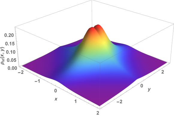
Figure 2: Behavior of the stationary distribution obtained from Eq. (19) with Green function given by Eq. (18). For simplicity, we consider the initial condition $\varphi(x,y)\propto e^{-x^{2}/\sigma_{x}^{2}-y^{2}/\sigma_{y}^{2}}/\left(\sigma_{x}\sigma_{y}\right)$, where $\sigma_{x}=\sigma_{y}=1/5$), $\sqrt{\alpha/D_{y}}=1$, and $\sqrt{\alpha/D_{x}}=1$ (in arbitrary units).

The MSD also carries information about the medium structure. We thus use the previous results to investigate how the MSD in each direction changes under those different scenarios. To do so and avoid transient behaviors related to the initial position of the walkers, we consider the initial condition $\varphi(x,y)=\delta(x)\delta(y)$. Under these assumptions, the MSD in the Laplace domain for each direction is

$$\bar{\sigma}_{y}^{2}(s)=\left\langle\left(y-\langle y\rangle\right)^{2}\right\rangle = 2\bar{{\cal{D}}}_{y}(s)/s\;\;\;{\text{and}}$$ (20)

$$\bar{\sigma}_{x}^{2}(s)=\left\langle\left(x-\langle x\rangle\right)^{2}\right\rangle = \bar{{\cal{D}}}_{x}(s)/\left(s\sqrt{\bar{{\cal{D}}}_{y}(s)}\right).$$ (21)

Equations (20) and (21) show that the MSD in the $y$-direction depends only on its memory kernel, while the MSD in the $x$-direction depends on both memory kernels. These features naturally emerge in the time-domain; indeed, by performing the inverse Laplace transform, we find

$$\sigma_{y}^{2}(t)=2\int_{0}^{t}dt^{\prime}\,{\cal{D}}_{y}(t^{\prime})\;\;\;{\text{and}}\;\;\;\sigma_{x}^{2}(t)=\frac{{\cal{D}}_{x}}{\sqrt{{\cal{D}}_{y}}}\int_{0}^{t}dt^{\prime}\,\zeta_{x,y}(t^{\prime})$$

where

$$\zeta_{x,y}(t)=\mathcal{L}^{-1}\left\{\frac{\bar{\mathcal{K}}_{x}(s)}{\sqrt{\bar{\mathcal{K}}_{y}(s)}}\right\}.$$ (22)

These dependencies are a direct consequence of the comb structure and are somehow related to the results of Ref. Ribeiro et al. (2014). The authors of that work have simulated fractional Brownian walks on a comb-like structure and reported that memory effects (associated with Hurst exponents) in $x$-direction do not affect the diffusive behavior in the $y$-direction; but, in the backbone, they found a nontrivial interplay between long-range memories in $x$ and $y$-directions.

We now consider the behavior of the system in each direction. To do so, we note that the Green function for the probability distribution function along the backbone $\mathcal{G}_{1}(x,t)=\int_{-\infty}^{\infty}dy\,\rho(x,y,t)$ satisfies the following generalized diffusion equation

$$\frac{\partial}{\partial t}\mathcal{G}_{1}(x,t)=\frac{\mathcal{D}_{x}}{2\sqrt{\mathcal{D}_{y}}}\frac{\partial}{\partial t}\int_{0}^{t}dt^{\prime}\,\zeta_{x,y}(t-t^{\prime})\frac{\partial^{2}}{\partial x^{2}}\mathcal{G}_{1}(x,t^{\prime})\;.$$ (23)

Similarly, the corresponding generalized diffusion equation for the Green function along the branches $\mathcal{G}_{2}(y,t)=\int_{-\infty}^{\infty}dx\,\rho(x,y,t)$ is

$$\frac{\partial}{\partial t}\mathcal{G}_{2}(y,t)=\mathcal{D}_{y}\frac{\partial}{\partial t}\int_{0}^{t}dt^{\prime}\,\mathcal{K}_{y}(t-t^{\prime})\frac{\partial^{2}}{\partial y^{2}}\mathcal{G}_{2}(y,t^{\prime}).$$ (24)

These two forms suggest that both Eqs. (23) and (24) have similar mathematical properties. By following Refs. Sandev et al. (2017b, 2018), we can verify that the probability distribution functions $\mathcal{G}_{1}(x,t)$ and $\mathcal{G}_{2}(y,t)$ are non-negative if: $1/\left[s\bar{\zeta}_{x,y}(s)\right]$ and $1/\left[s\bar{\mathcal{K}}_{y}(s)\right]$ are completely monotone functions; and $1/\bar{\zeta}_{x,y}(s)$ and $1/\bar{\mathcal{K}}_{y}(s)$ are Bernstein functions. Moreover, by following the results of Ref. Sokolov (2001), we can further verify that Eqs. (23) and (24) fulfill the Nyquist theorem, and consequently, their solutions are thermodynamically sound.

To investigate the interplay between mechanisms of annealed (memory kernels) and quenched (comb-like structure) disorders, we start considering several definitions for the fractional time operators. For the sake of comparison, it is worth remembering that ordinary derivatives (usual comb-model) imply in $\mathcal{K}_{x}(t)=\mathcal{K}_{y}(t)=\delta(t)$, that in turn lead to $\sigma_{y}^{2}(t)\propto t$ and $\sigma_{x}^{2}(t)\propto t^{1/2}$ Arkhincheev and Baskin (1991).

We first consider the Riemann-Liouville operator, yielding the kernels $\bar{{\cal{K}}}_{\alpha_{x}}(s)\propto 1/s^{\alpha_{x}}$ ($0<\alpha_{x}<1$) and $\bar{{\cal{K}}}_{\alpha_{y}}(s)\propto 1/s^{\alpha_{y}}$ ($0<\alpha_{y}<1$). These memory kernels are related to the Green function given by Eq. (II), and their corresponding MSDs are

$$\sigma_{y}^{2}(t) = 2\mathcal{D}_{y}\,\mathcal{L}^{-1}\left\{s^{-\alpha_{y}-1}\right\}=2\mathcal{D}_{y}\frac{t^{\alpha_{y}}}{\Gamma(1+\alpha_{y})}\;\;\;\;\ \text{and}$$ (25)

$$\sigma_{x}^{2}(t) = \frac{\mathcal{D}_{x}}{\sqrt{\mathcal{D}_{y}}}\mathcal{L}^{-1}\left\{s^{-\alpha_{x}+\alpha_{y}/2-1}\right\}=\frac{\mathcal{D}_{x}}{\sqrt{\mathcal{D}_{y}}}\frac{t^{\alpha_{x}-\alpha_{y}/2}}{\Gamma(1+\alpha_{x}-\alpha_{y}/2)}.$$ (26)

Equation (25) shows that the diffusion in branches is independent of the backbone dynamics; it only depends on its memory effects. However, the MSD in the backbone depends on memory effects in both directions, as shown in Eq. (26).

By imposing the conditions of non-negativity to the corresponding solution, we find that $\alpha_{x}>\alpha_{y}/2$. To better understand this condition, let us examine some limiting cases. When $\alpha_{x}=1$ (ordinary derivative in the backbone) and $0<\alpha_{y}<1$ (memory effects in the branches), the backbone diffusion is enhanced if $1/2<1-\alpha_{y}/2<1$. This result is intriguing and counter-intuitive because, as the branches act like traps, we could initially presume that the slower the diffusion in the branches, the more subdiffusive is the diffusion on the backbone; but quite the opposite happens. When the spread over the branches is subdiffusive, the walkers stay closer to the backbone and their probability of returning to the backbone increases, enhancing the diffusion in the $x$-direction. This phenomenon is related to the so-called “subdiffusion paradox” reported in cell environments Sereshki et al. (2012); Barkai et al. (2012); Barr et al. (2015). Although subdiffusion reduces the exploration area, it increases the likelihood of walkers to stay close to specific targets Golding and Cox (2006); Guigas and Weiss (2008). In contrast, for $1/2<\alpha_{x}<1$ (memory effects in the backbone) and $\alpha_{y}=1$ (ordinary derivative in the branches), the spread in the backbone is even more subdiffusive if $0<\alpha_{x}-1/2<1/2$. Thus, the backbone subdiffusion is governed by the interplay of two mechanisms: the trapping in the branches and the memory effects in the backbone. Furthermore, an essential feature of Eqs. (25) and (26) is scale invariance, that is, the effects of geometrical restrictions and memory effects are the same in all time-scales. This last behavior is illustrated in Figure 3 for $\alpha_{x}=1$ and $\alpha_{y}=1$ (solid black line).

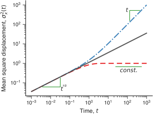
Figure 3: Behavior of the MSD $\sigma_{x}^{2}$ versus $t$ for different kernels. The solid black line refers to subdiffusion when $\bar{{\cal{K}}}_{x}(s)\propto 1/s^{\alpha_{x}}$ and $\bar{{\cal{K}}}_{y}(s)\propto 1/s^{\alpha_{y}}$, where we have chosen ${\cal{D}}_{x}/\sqrt{{\cal{D}}_{y}}=1$, $\alpha_{x}=1$, and $\alpha_{y}=1$. The dot-dashed blue line corresponds to usual diffusion obtained as the asymptotic behavior for $\bar{{\cal{K}}}_{x}(s)\propto 1/s^{\alpha_{x}}$ and $\bar{{\cal{K}}}_{y}(s)\propto 1/\left(s+\alpha^{\prime}_{y}\right)$, where, for simplicity, we have chosen ${\cal{D}}_{x}/\sqrt{{\cal{D}}_{y}{\cal{R}}(\alpha_{y})}=1$, $\alpha_{x}=1$, and $\alpha_{y}=1$. The dashed red line corresponds to $\bar{{\cal{K}}}_{x}(s)\propto 1/(s+\alpha_{x})$ with $\bar{{\cal{K}}}_{y}(s)\propto 1/(s+\alpha_{y})$ (the case with stationary state), where we have chosen ${\cal{R}}(\alpha_{x}){\cal{D}}_{x}/\sqrt{{\cal{D}}_{y}{\cal{R}}(\alpha_{y}})=1$, $\alpha_{x}=1$, and $\alpha_{y}=1$.

As a second example, we investigate an anisotropic case characterized by different memory kernels for $x$ and $y$ directions. We maintain the same power-law kernel for the backbone, that is, ${\cal{K}}_{\alpha_{x}}(s)\propto 1/s^{\alpha_{x}}$ (with $1/2\leq\alpha_{x}<1$ to ensure non-negative solutions), and consider an exponential memory kernel ${\cal{K}}_{\alpha_{y}}(s)\propto 1/\left(s+\alpha^{\prime}_{y}\right)$ for the branches, with $\alpha^{\prime}_{y}=\alpha_{y}/(1-\alpha_{y})$ and $0<\alpha_{y}<1$. These choices correspond to the Riemann-Liouville fractional operator in the $x$-direction and the Caputo-Fabrizio operator in the $y$-direction. Under these conditions, we find the MSDs

$$\sigma_{y}^{2}(t) = 2D_{y}\,\mathcal{L}^{-1}\left\{\frac{s^{-1}}{s+\alpha^{\prime}_{y}}\right\}=2\frac{D_{y}}{\alpha^{\prime}_{y}}\left(1-e^{-\alpha^{\prime}_{y}t}\right)\;\;\;\text{and}\;\;\;$$ (27)

$$\sigma_{x}^{2}(t) = \frac{\mathcal{D}_{x}}{\sqrt{D_{y}}}\mathcal{L}^{-1}\left\{\frac{s^{-\alpha_{x}-1}}{\left(s+\alpha^{\prime}_{y}\right)^{-1/2}}\right\}=\frac{\mathcal{D}_{x}}{\sqrt{D_{y}}}t^{\alpha_{x}-1/2}E_{1,\alpha_{x}+1/2}^{-1/2}(-\alpha_{y}t),$$ (28)

where

$$E_{\alpha,\beta}^{\delta}(z)=\sum_{k=0}^{\infty}\frac{(\delta)_{k}}{\Gamma(\alpha k+\beta)}\frac{z^{k}}{k!}$$ (29)

is the three-parameter Mittag-Leffler function Prabhakar (1971), and $(\delta)_{k}=\Gamma(\gamma+k)/\Gamma(\gamma)$ represents the Pochhammer symbol Prabhakar (1971). For the calculations of Eqs. (27) and (28) we have used that Prabhakar (1971)

$$\mathcal{L}\left\{t^{\beta-1}E_{\alpha,\beta}^{\delta}(-\nu t^{\alpha})\right\}(s)=\frac{s^{\alpha\delta-\beta}}{\left(s^{\alpha}+\nu\right)^{\delta}},$$ (30)

where $\Re(s)>|\nu|^{1/\alpha}$.

Equation (27) shows the isolated effects of the exponential memory kernel. We notice that the exponential term approaches zero for long times, and the MSD thus reaches a plateau of saturation. This behavior describes a confined (localized, restricted, or corralled) diffusion, where $\alpha^{\prime}_{y}$ can be associated with a saturation rate, and the asymptotic value of the MSD represents the magnitude of the confinement region. MSDs having the general form of Eq. (27), that is,

$$\sigma^{2}(t)=A_{\infty}(1-e^{-\xi t}),$$ (31)

are well-known to emerge in Ornstein-Uhlenbeck processes Wang and Uhlenbeck (1945) and restricted diffusion confined within reflecting boundaries Kusumi et al. (1993). However, the restricted diffusion observed here occurs without external forces or finite boundary conditions, a remarkable feature of the Caputo-Fabrizio operator that has also been reported in Ref. Tateishi et al. (2017).

The confined diffusion observed in Eq. (31) suggests a relationship between the exponential kernels and stationary states (stochastic localization phenomena). Indeed, the same equation emerges in the work Méndez and Campos Méndez and Campos (2016), where a CTRW model for diffusion with resetting (walkers return to the origin with a resetting probability $r$) was proposed. A connection between fractional diffusion equations with the Caputo-Fabrizio operator and diffusion with stochastic resetting was also established in Ref. Tateishi et al. (2017). Méndez and colleagues Méndez et al. (2015) also studied a CTRW on a comb structure subjected to a bias parameter on the branches, where Eq. (31) appears as an asymptotic behavior for the backbone diffusion when the walker is biased to stay along the branches. The authors of Ref. Ribeiro et al. (2014) verified that normal diffusion emerges on the backbone when a fractional Brownian motion with long-range anti-persistent correlations occurs on the branches. By studying a minimal random walk model with infinite memory (walkers preferentially return to previously visited sites), Boyer and Solis-Salas Boyer and Solis-Salas (2014) established a connection between long-range memory and stationary states of MSD and demonstrated how to infer memory strength use in animals (monkeys).

In this context, we can verify whether the relation between the Caputo-Fabrizio operator and confined diffusion is valid for the comb-model from the evolution of Eq. (28). To do so, we calculate the asymptotic limits of Eqs. (27) and (28) for short- and long-times, that is,

$$\sigma_{y}^{2}(t) \sim 2\mathcal{D}_{y}\,\left\{\begin{array}[]{c l}\alpha^{\prime}_{y}t,&t\rightarrow 0,\\ 1,&t\rightarrow\infty,\end{array}\right.~{}~{}\text{and}$$ (34)

$$\sigma_{x}^{2}(t) \sim \frac{\mathcal{D}_{x}}{\sqrt{D_{y}}}\left\{\begin{array}[]{c l}\frac{t^{\alpha_{x}-1/2}}{\Gamma(\alpha_{x}+1/2)},&t\rightarrow 0,\\ \frac{t^{\alpha_{x}}}{\Gamma(\alpha_{x}+1)},&t\rightarrow\infty.\end{array}\right.$$ (37)

In previous calculations, we use the formula Sandev et al. (2015b); Garra and Garrappa (2018)

$$E_{\alpha,\beta}^{\delta}(-z)=\frac{z^{-\delta}}{\Gamma(\delta)}\sum_{k=0}^{\infty}\frac{\Gamma(\delta+k)}{\Gamma(\beta-\alpha(\delta+n))}\frac{(-z)^{-n}}{n!},$$ (38)

for $0<\alpha<2$ and $z\rightarrow\infty$, from which we find the asymptotic behavior

$$E_{\alpha,\beta}^{\delta}(-t^{\alpha})\simeq\frac{t^{-\alpha\delta}}{\Gamma(\beta-\alpha\delta)},\quad t\rightarrow\infty.$$ (39)

Equations (34) and (37) show that Brownian motion governs the branches dynamics at short-times, promoting enhanced subdiffusion in the backbone with $0<\alpha^{\prime}_{x}-1/2<1/2$ and $\alpha^{\prime}_{y}=1$ (as discussed earlier). In the long-time limit, a stationary state emerges in the branches, and the backbone dynamics only depends on its power-law memory kernel. In particular, there is a crossover from subdiffusion ($\sigma_{x}^{2}(t)\propto t^{1/2}$) to Brownian diffusion ($\sigma_{x}^{2}(t)\propto t$) when $\alpha_{x}=1$ (dot-dashed blue line in Figure 3). We thus find an intriguing result where the interplay between geometrical restriction and memory effects (mechanisms associated with subdiffusion) produces usual Brownian motion. Similar behavior also emerges for power-law memory kernels when $\alpha_{x}\rightarrow 1$ and $\alpha_{y}\rightarrow 0$, for suitable combinations of Hurst exponents in fractional Brownian motions over a comb structure (Figure 5 of Ref. Ribeiro et al. (2014)), and without memory effects when the branches of the comb are finite Havlin and Ben-Avraham (2002); Berezhkovskii et al. (2015); Arkhincheev (2007). However, the results of Eqs. (34) and (37) are obtained with no memory effects in the $x$-direction and the stationary state is a consequence of the exponential memory kernel valid for $0<\alpha^{\prime}_{y}<1$.

The crossover is an essential feature of our model and provides insights into the time scale that each mechanism of subdiffusion is most relevant. As we already discussed, the dynamics in short-times is the same as the usual comb-model; therefore, subdiffusion is caused by geometrical restrictions. On the other hand, the exponential memory kernel produces a dynamics similar to a random walk with a high probability of returning to the origin. Since the backbone is at the origin, walkers along the branches tend to stay confined near the backbone because of memory effects, which in turn produces Brownian diffusion on the backbone. The memory effects along the branches thus dominate longer time scales. This interpretation is somehow in agreement with the results on anisotropic diffusion of entangled biofilaments reported in Ref. Tsang et al. (2017), where the authors have written: “The physical reason is that linear macromolecules become transiently localized in directions transverse to their backbone but diffuse with relative ease parallel to it.” In particular, they obtained an empirical MSD $\sim t^{0.2}$ for the transversal direction and a MSD $\sim t^{0.9}$ for the parallel direction of such macromolecules. Liang Hong and co-workers also reported a gradual crossover from subdiffusion to Brownian diffusion on the mobility of water molecules on protein surfaces Tan et al. (2018). They further argued that a broad distribution of trapping times causes the subdiffusion; however, water molecules start jumping to the empty sites as the trappings become occupied, resulting in the Brownian diffusion.

We can further investigate the effects of exponential memory kernels simultaneously acting on the backbone and branches, that is, $\bar{{\cal{K}}}_{\alpha_{x}}(s)\propto 1/(s+\alpha^{\prime}_{x})$ and $\bar{{\cal{K}}}_{\alpha_{y}}(s)\propto 1/(s+\alpha^{\prime}_{y})$. These memory kernels are related to the Green functions given by Eqs. (II) and (18), where $\alpha^{\prime}_{x}=\alpha^{\prime}_{y}=\alpha$ is also a condition ensuring the non-negativity of the corresponding solution. If our interpretation of the exponential memory kernel is valid, we expected stationary states to emerge even in the backbone dynamics. This hypothesis is corroborated by Figure 2 and the results for MSD

$$\sigma_{y}^{2}(t) = 2\mathcal{D}_{y}\,\mathcal{L}^{-1}\left\{\frac{s^{-1}}{s+\alpha}\right\}=2\frac{D_{y}}{\alpha}\left(1-e^{-\alpha t}\right)\;\;\;\text{and}$$ (40)

$$\sigma_{x}^{2}(t) = \frac{D_{x}}{\sqrt{D_{y}}}\mathcal{L}^{-1}\left\{\frac{\sqrt{s+\alpha}}{s(s+\alpha)}\right\}=\frac{D_{x}}{\sqrt{D_{y}}}\frac{1}{\sqrt{\alpha}}\mathrm{erf}\left(\sqrt{\alpha t}\right),$$ (41)

where $\mathrm{erf}(x)$ is the error function. These results show that the behavior on both directions reaches a stationary state for long times, that is, $\sigma_{y}^{2}(t)$ and $\sigma_{x}^{2}(t)$ approach a constant plateau when $t\rightarrow\infty$. Figure 3 shows the behavior of $\sigma_{x}^{2}(t)$ for different time scales (dashed red line). Once again, a crossover characterizes the backbone dynamics and the system evolves from subdiffusion to confined diffusion (stationary state). The quenched mechanism dominates at short-time scales and the annealed mechanism predominates in the long-run. It is noteworthy that confined diffusion on both $x$ and $y$ directions has been experimentally observed in the crowded environment of living cells such as in lateral diffusion of membrane receptors Kusumi et al. (1993) and diffusion of protein aggregates in live E. coli cells Coquel et al. (2013).

III Generalized Fractal Structure of Backbones

We now focus on generalizing the quenched disorder mechanism of the comb-model (Eq. 2) by changing its geometrical restrictions. Instead of multiplying the diffusion term in the $x$-direction by a single delta function $\delta(y)$, we consider a multiplication by $\sum_{l_{j}\in\mathcal{S}_{\nu}}\delta(y-l_{j})$ to obtain an infinite number of backbones, where the position of the backbones $l_{j}$ $(j=1,2,\dots)$ belong to a fractal set $\mathcal{S}_{\nu}$ with fractal dimension $0<\nu<1$. These geometrical restrictions characterize a fractal grid Sandev et al. (2015a, 2016a, 2017a), as illustrated in Figure 4 for the one-third Cantor set ($\nu\simeq 0.631$) at the third step of the iteration. Under these conditions, the diffusion equation for the fractal comb-model is

$$\frac{\partial}{\partial t}\rho(x,y;t)={\cal{F}}_{t,y}\left({\cal{D}}_{y}\frac{\partial^{2}}{\partial y^{2}}\rho(x,y;t)\right)+\sum_{l_{j}\in\mathcal{S}_{\nu}}\delta(y-l_{j}){\cal{F}}_{t,x}\left({\cal{D}}_{x}\frac{\partial^{2}}{\partial x^{2}}\rho(x,y;t)\right).$$ (42)

We proceed by defining the generalized diffusion equation governing the dynamics on the backbones. By applying the Laplace transform in Eq. (42), we have

$$\!\!\!\!s\bar{\rho}(x,y;s)-\varphi(x,y)=s{\cal{D}}_{y}\bar{\mathcal{K}}_{y}(s)\frac{\partial^{2}}{\partial y^{2}}\bar{\rho}(x,y;s)+\sum_{l_{j}\in\mathcal{S}_{\nu}}\delta(y-l_{j})s{\cal{D}}_{x}\bar{\mathcal{K}}_{x}(s)\frac{\partial^{2}}{\partial x^{2}}\bar{\rho}(x,y;s).$$ (43)

By following the procedures of Ref. Sandev et al. (2016a) and considering a suitable initial condition, we can represent the probability distribution function as

$$\bar{\rho}(x,y;s)=\bar{f}(x,s)\exp\left(-\frac{|y|}{\sqrt{\mathcal{D}_{y}\bar{\mathcal{K}}_{y}(s)}}\right).$$ (44)

Note that the exponential term carries information about the diffusion in the branches. From Eq. (44), we find a relation for the probability distribution of the $x$-direction in the Laplace domain, that is,

$$\bar{\mathcal{G}}_{1}(x;s)=2\sqrt{\mathcal{D}_{y}\bar{\mathcal{K}}_{y}(s)}\bar{f}(x,s).$$ (45)

On the other hand, we also have that $\bar{\mathcal{G}}_{1}(x,t)=\int_{-\infty}^{\infty}dy\,\bar{\rho}(x,y,t)$ and by integrating Eq. (43), we find

$$s\bar{\mathcal{G}}_{1}(x;s)-\Phi(x)=s{\cal{D}}_{x}\bar{\mathcal{K}}_{x}(s)\frac{\partial^{2}}{\partial x^{2}}\sum_{l_{j}\in\mathcal{S}_{\nu}}\bar{\rho}(x,y=l_{j};s)\;,$$ (46)

where $\Phi(x)=\int_{-\infty}^{\infty}dy\,\varphi(x,y)$, and $\bar{\rho}(x,y=l_{j};s)$ represents the probability distribution function for the backbone in the position $l_{j}$.

Figure 4: Example of a fractal comb structure. The one-third Cantor set (at the third step of construction) provides the rule to locate the backbones perpendicularly to the $y$-axis. The location of the branches is distributed continuously along the backbones, that is, walkers access the branches through any position on the backbones. This spatial configuration characterizes a fractal grid.

The summation $\sum_{l_{j}\in\mathcal{S}_{\nu}}\bar{\rho}(x,y=l_{j};s)$ can be formally replaced by integration to fractal measure $\mu_{\nu}\sim l^{\nu}$, where $\sum_{l_{j}\in\mathcal{S}_{\nu}}\delta(l-l_{j})\rightarrow\frac{1}{\Gamma(\nu)}l^{\nu-1}$ is the fractal density, that is, $d\mu_{\nu}=\frac{1}{\Gamma(\nu)}l^{\nu-1}\,dl$ Tarasov (2004). Therefore, from Eqs. (44) and (45), we obtain

$$\sum_{l_{j}\in\mathcal{S}_{\nu}}\bar{\rho}(x,y=l_{j};s) = \sum_{l_{j}\in\mathcal{S}_{\nu}}\bar{f}(x,s)\exp\left(-\frac{|l_{j}|}{\sqrt{\mathcal{D}_{y}\bar{\mathcal{K}}_{y}(s)}}\right)$$ (47)

$$= \bar{f}(x,s)\frac{1}{\Gamma(\nu)}\int_{0}^{\infty}dl\,l^{\nu-1}e^{-\frac{l}{\sqrt{\mathcal{D}_{y}\bar{\mathcal{K}}_{y}(s)}}}$$

$$= \bar{f}(x,s)\left[\mathcal{D}_{y}\bar{\mathcal{K}}_{y}(s)\right]^{\nu/2}=\frac{1}{2\mathcal{D}_{y}^{\frac{1-\nu}{2}}}\left[\bar{\mathcal{K}}_{y}(s)\right]^{-\frac{1-\nu}{2}}\bar{\mathcal{G}}_{1}(x;s).$$

We observe in Eq. (47) that the power-law exponents of the diffusion coefficient and memory kernel of $y$-direction contains all information about the fractal structure of backbones. Hence, by using the result of Eq. (47) in Eq. (46), we find

$$s\bar{\mathcal{G}}_{1}(x;s)-\Phi(x)=\frac{\mathcal{D}_{x}}{2\mathcal{D}_{y}^{\frac{1-\nu}{2}}}s\frac{\bar{\mathcal{K}}_{x}(s)}{\left[\bar{\mathcal{K}}_{y}(s)\right]^{\frac{1-\nu}{2}}}\frac{\partial^{2}}{\partial x^{2}}\bar{\mathcal{G}}_{1}(x;s).$$ (48)

The inverse Laplace transform of Eq. (48) yields the generalized diffusion equation

$$\frac{\partial}{\partial t}\mathcal{G}_{1}(x;t)=\left(\frac{\mathcal{D}_{x}}{2\mathcal{D}_{y}^{\frac{1-\nu}{2}}}\right)\frac{\partial}{\partial t}\int_{0}^{t}dt^{\prime}\,\eta(t-t^{\prime})\frac{\partial^{2}}{\partial x^{2}}\mathcal{G}_{1}(x;t^{\prime}),$$ (49)

where the memory kernel $\eta(t)$ depends on both annealed and quenched disorder mechanisms, as given by

$$\eta(t)=\mathcal{L}^{-1}\left\{\frac{\bar{\mathcal{K}}_{x}(s)}{\left[\bar{\mathcal{K}}_{y}(s)\right]^{\frac{1-\nu}{2}}}\right\}.$$ (50)

By using Eq. (49), we obtain the general expression for the MSD of a comb structure related to the fractal dimension $0<\nu<1$ in the Laplace domain, that is,

$$\sigma_{x}^{2}(t)=2\left(\frac{\mathcal{D}_{x}}{2\mathcal{D}_{y}^{\frac{1-\nu}{2}}}\right)\mathcal{L}^{-1}\left\{\frac{\bar{\mathcal{K}}_{x}(s)}{s[\bar{\mathcal{K}}_{y}(s)]^{\frac{1-\nu}{2}}}\right\}.$$ (51)

We note again that probability distributions along the backbones structure should be non-negative; therefore: $1/\left[s\bar{\eta}(s)\right]=\left[\bar{\mathcal{K}}_{y}(s)\right]^{\frac{1-\nu}{2}}/\left[s\bar{\mathcal{K}}_{x}(s)\right]$ should be completely monotone function, and $1/\bar{\eta}(s)=\left[\bar{\mathcal{K}}_{y}(s)\right]^{\frac{1-\nu}{2}}/\bar{\mathcal{K}}_{x}(s)$ should be a Bernstein function.

To investigate the isolated effects of geometrical restrictions of the fractal grid, we consider the case $\bar{\mathcal{K}}_{x}(t)=\bar{\mathcal{K}}_{y}(t)=1$ (that is, $\bar{\mathcal{K}}_{x}(s)=\bar{\mathcal{K}}_{y}(s)=1/s$) where the MSD recovers the result of Ref. Sandev et al. (2015a), that is,

$$\sigma_{x}^{2}(t)=2\left(\frac{\mathcal{D}_{x}}{2\mathcal{D}_{y}^{\frac{1-\nu}{2}}}\right)\mathcal{L}^{-1}\left\{\frac{s^{-1}}{s^{1-\frac{1-\nu}{2}}}\right\}=2\frac{\mathcal{D}_{x}}{2\mathcal{D}_{y}^{\frac{1-\nu}{2}}}\frac{t^{\frac{1+\nu}{2}}}{\Gamma\left(1+\frac{1+\nu}{2}\right)}.$$ (52)

The power-law behavior ($\sigma_{x}^{2}(t)\simeq t^{\frac{1+\nu}{2}}$) indicates a scale invariance, and because the exponent depends on $\nu$, we infer that the fractal grid affects the spreading dynamics in all time scales. The overall effect is a subdiffusive dynamics with $\frac{1}{2}<\frac{1+\nu}{2}<1$; however, the subdiffusion in a fractal grid is faster than the usual comb-model ($\sigma_{x}^{2}(t)\simeq t^{1/2}$ Arkhincheev and Baskin (1991), corresponding to $\nu=0$ in our case). This behavior occurs because the set of backbones increases the possibilities of diffusion in the $x$-direction. For example, a fractal grid with $\nu\simeq 0.631$ (the one-third Cantor set) implies in $\sigma_{x}^{2}(t)\simeq t^{0.816}$. Moreover, Eq. (52) connects the anomalous diffusion exponent with the fractal dimension of the backbone structure, a result that was experimentally observed in diffusion in porous and structurally inhomogeneous media Zhokh et al. (2018).

One example of the interplay between this generalized geometrical restriction and the effect of memory kernels is given by $\bar{\mathcal{K}}_{x}(s)=\bar{\mathcal{K}}_{y}(s)=1/s^{\alpha}$. This choice yields a fractional diffusion equation for a fractal grid given by

$$\frac{\partial}{\partial t}\rho(x,y;t)={{}_{RL}}D_{t}^{1-\alpha}\left[{\cal{D}}_{y}\frac{\partial^{2}}{\partial y^{2}}\rho(x,y;t)+{\cal{D}}_{x}\sum_{l_{j}\in\mathcal{S}_{\nu}}\delta(y-l_{j})\frac{\partial^{2}}{\partial x^{2}}\rho(x,y;t)\right]\,,$$ (53)

and whose MSD is

$$\sigma_{x}^{2}(t)=2\left(\frac{\mathcal{D}_{x}}{2\mathcal{D}_{y}^{\frac{1-\nu}{2}}}\right)\mathcal{L}^{-1}\left\{s^{-\frac{\alpha+\nu}{2}-1}\right\}=2\left(\frac{\mathcal{D}_{x}}{2\mathcal{D}_{y}^{\frac{1-\nu}{2}}}\right)\frac{t^{\frac{\alpha+\nu}{2}}}{\Gamma\left(\frac{\alpha+\nu}{2}\right)}.$$ (54)

The power-law exponent $\frac{\alpha+\nu}{2}$ is associated with the two anomalous diffusion mechanisms: memory effects (related to $\alpha$) and the fractal structure restriction (given by $\nu$). The interplay between these mechanisms produces subdiffusive regimes between the limit cases of restricted and Brownian diffusion, that is, $0<\frac{\alpha+\nu}{2}<1$. The case of a single backbone ($\nu=0$) yields $\sigma_{x}^{2}(t)\simeq t^{\alpha/2}$, as reported in Ref. Sandev et al. (2016b). From the general formula of Eq. (51), we further conclude that the MSD along the $x$-direction is stationary (case of localization) if $\bar{\mathcal{K}}_{x}(s)\propto\left[\bar{\mathcal{K}}_{y}(s)\right]^{\frac{1-\nu}{2}}$, and that normal diffusion along the $x$-direction occurs for $\bar{\mathcal{K}}_{x}(s)\propto s^{-1}\left[\bar{\mathcal{K}}_{y}(s)\right]^{\frac{1-\nu}{2}}$. A remarkable feature of these conditions is that both memory kernels must have the same effects of geometrical restrictions.

IV Discussion and Conclusions

Over this work, we showed that our generalized comb-models account for annealed and quenched disorder mechanisms. We believe these comb-models with fractional time-derivative operators are a reasonable abstraction for systems where the interplay between temporal and spatial disorders is present. For these hybrid models, we considered different memory kernels for the backbone and branch structures, and a fractal generalization of the geometrical restrictions. We obtained general solutions for the diffusion propagator and the MSD in terms of these memory kernels. With these solutions, we discussed particular cases based on the temporal evolution of the MSD and inferred time scales associated with each disorder mechanism. These results thus provide theoretical knowledge about the importance of interactions between geometrical restrictions and memory effects on anomalous diffusion.

We argued that the behaviors obtained from our models are consistent with other theoretical and experimental results. In its usual form, the comb-model is a subdiffusive model with $\sigma_{x}^{2}\propto t^{1/2}$. However, depending on the memory kernels and number of backbones (single or fractal set), our generalized comb-models also describe restricted diffusion, Brownian diffusion, and display a crossover from subdiffusion to these situations.

For power-law memory kernels, the MSD is scale-invariant and the diffusive regime depends on the values of memory exponents $0<\alpha_{x}<1$ and $0<\alpha_{y}<1$ with $\alpha_{x}>\alpha_{y}/2$. Scale invariance is also a feature of the fractal grid structure of backbones. In this case, there is an enhancement of the diffusion (when compared with the usual comb-model) and the anomalous exponent depends on the fractal dimension ($\frac{1}{2}<\frac{1+\nu}{2}<1$). By including power-law memory effects on the fractal grid, we obtained an anomalous exponent $0<\frac{\alpha+\nu}{2}<1$ with $\alpha=\alpha_{x}=\alpha_{y}$. Overall, these results from our generalized comb-models are consistent with simulations of fractal Brownian motion Ribeiro et al. (2014) and a biased CTRW Méndez et al. (2015) on comb-like structures.

When the memory kernel acting on the branches is exponential, we showed that the behavior of the MSD in the $y$-direction is similar to those reported in diffusion with explicit confinement (external forces or limited boundaries) or having a bias to return to the origin. The spread in the branches thus follows Brownian diffusion for short-time scales and becomes confined near to the backbone for long times. Because of this high probability of returning to the backbone, the long-time behavior in $x$-direction only depends on its memory kernel. The overall effect of an exponential kernel is a crossover between diffusive regimes. This crossover occurs from subdiffusion to Brownian diffusion when walkers have no memory in the backbone. Thus, we observed that the interplay between two subdiffusion mechanisms (geometrical restrictions and memory effects) may lead to the usual Brownian motion. This crossover and its physical explanation also appear consistent with experimental results of anisotropic diffusion of entangled biofilaments Tsang et al. (2017) and the mobility of water molecules on protein surfaces Tan et al. (2018). On the other hand, when an exponential memory kernel acts on the backbone, we obtained a crossover from subdiffusion to confined diffusion. This result also appears consistent with the MSD observed in lateral diffusion of membrane receptors Kusumi et al. (1993) and diffusion of protein aggregates in live E. coli cells Coquel et al. (2013). Moreover, we found that the confinement effects of exponential memory kernels are independent of the parameters $\alpha^{\prime}_{y}$ and $\alpha^{\prime}_{x}$.

In spite of its simplicity, our generalized comb-model may have an important role in the statistical mechanics of disordered media. This model can be used as a simple explanation for unusual transport properties caused by quenched disorder or to annealed disorder. It also has the advantage of providing exact solutions related to sub- and superdiffusive behaviors. Our comb-models are also relevant for investigating the interplay between temporal and spatial disorder mechanisms and for describing crossovers from subdiffusion to confined or Brownian diffusion.

References

- Perrin (1910) J. Perrin, Brownian Movement and Molecular Reality (Taylor and Francis, London, 1910).
- Lévy (1954) P. Lévy, Proc. Int. Congress of Math. 3, 416 (1954).
- Smith (1955) W. L. Smith, Proc. Roy. Soc. Ser. A 232, 6 (1955).
- Montroll and Weiss (1965) E. W. Montroll and G. H. Weiss, J. Math. Phys. 6, 167 (1965).
- Scher and Lax (1973a) H. Scher and M. Lax, Phys. Rev. B 7, 4491 (1973a).
- Scher and Lax (1973b) H. Scher and M. Lax, Phys. Rev. B 7, 4502 (1973b).
- Kutner and Masoliver (2017) R. Kutner and J. Masoliver, Eur. Phys. J. B 50, 90 (2017).
- Klafter et al. (1987) J. Klafter, A. Blumen, and M. F. Shlesinger, Phys. Rev. A 35, 3081 (1987).
- Hilfer and Anton (1995) R. Hilfer and L. Anton, Phys. Rev. E 51, R848 (1995).
- Compte (1996) A. Compte, Phys. Rev. E 53, 4191 (1996).
- Barkai (2002) E. Barkai, Chem. Phys. 284, 13 (2002).
- Meztler and Klafter (2000) R. Meztler and J. Klafter, Phys Rep. 339, 1 (2000).
- West (2016) B. J. West, Fractional Calculus View of Complexity: Tomorrow’s Science (CRC Press, London, 2016).
- Broadbent and Hammersley (1957) S. Broadbent and J. Hammersley, Math. Proc. Cambridge 53, 629 (1957).
- Havlin and Ben-Avraham (2002) S. Havlin and D. Ben-Avraham, Adv. Phys. 51, 187 (2002).
- de Gennes (1976) P. G. de Gennes, La Recherche 7, 919 (1976).
- Bouchaud and Georges (1990) J. P. Bouchaud and A. Georges, Phys. Rep. 195, 127 (1990).
- Bok et al. (2009) J. Bok, J. Prost, and F. Brochard-Wyart, P.G. De Gennes’ Impact on Science – Volume I: Solid State and Liquid Crystals (World Scientific, 2009).
- Mandelbrot and Blumen (1989) B. B. Mandelbrot and A. Blumen, Proc. R. Soc. Lond. A 423, 3 (1989).
- Sen (2004) P. N. Sen, Concepts Magn. Reson. A23, 1 (2004).
- Waigh (2005) T. A. Waigh, Rep. Prog. Phys. 68, 685 (2005).
- Kirstein et al. (2007) J. Kirstein, B. Platschek, C.Jung, R. Brown, T. Bein, and C. Bräuchle, Nat. Mater. 6, 303 (2007).
- Wirtz (2009) D. Wirtz, Annu. Rev. Biophys. 38, 301 (2009).
- Novikov et al. (2014) D. S. Novikov, J. H. Jensen, J. A. Helpern, and E. Fieremans, Proc. Natl. Acad. Sci. USA 111, 5088 (2014).
- Papaioannou et al. (2017) A. Papaioannou, D. S. Novikov, E. Fieremans, and G. S. Boutis, Phys. Rev. E 96, 061101(R) (2017).
- Assaf et al. (2019) Y. Assaf, H. Johansen-Berg, and M. T. de Schotten, NMR Biomed. 32, e3762 (2019).
- Song et al. (2019) S. Song, S. J. Park, M. Kim, J. S. Kim, B. J. Sung, S. Lee, J.-H. Kim, and J. Sung, Proc. Natl. Acad. Sci. USA 116, 12733 (2019).
- Metzler (2017) R. Metzler, Biophys J. 112, 413 (2017).
- Meroz et al. (2010) Y. Meroz, I. M. Sokolov, and J. Klafter, Phys. Rev. E 81, 010101(R) (2010).
- Weigel et al. (2011) A. V. Weigel, B. Simon, M. M. Tamkun, and D. Krapfa, Proc. Natl. Acad. Sci. USA 108, 6438 (2011).
- Jeon et al. (2011) J.-H. Jeon, V. Tejedor, S. Burov, E. Barkai, C. Selhuber-Unkel, K. Berg-Sørensen, L. Oddershede, and R. Metzler, Phys. Rev. Lett. 106, 048103 (2011).
- Tabei et al. (2013) S. M. A. Tabei, S. Burov, H. Y. Kim, A. Kuznetsov, T. Huynh, J. Jureller, L. H. Philipson, A. R. Dinner, and N. F. Scherer, Proc. Natl. Acad. Sci USA 110, 4911–4916 (2013).
- Miyaguchi and Akimoto (2015) T. Miyaguchi and T. Akimoto, Phys. Rev. E 91, 010102(R) (2015).
- Golan and Sherman (2017) Y. Golan and E. Sherman, Nat. Commun. 8, 15851 (2017).
- Furnival et al. (2017) T. Furnival, R. K. Leary, E. C. Tyo, S.Vajda, Q. M. Ramasse, J. M. Thomas, P. D. Bristowe, and P. A. Midgleya, Chem. Phys. Lett. 683, 370 (2017).
- Coniglio (1981) A. Coniglio, Phys. Rev. Lett. 46, 250 (1981).
- Stanley and Coniglio (1984) H. E. Stanley and A. Coniglio, Phys. Rev. B 29, 522(R) (1984).
- White and Barma (1984) S. R. White and M. Barma, Phys. A: Math. Gen. 17, 2995 (1984).
- Havlin et al. (1987) S. Havlin, J. E. Kiefer, and G. H. Weiss, Phys. Rev. A 36, 1403 (1987).
- Arkhincheev and Baskin (1991) V. E. Arkhincheev and E. M. Baskin, Sov. Phys. JETP 73, 161 (1991).
- Arkhincheev (1999) V. E. Arkhincheev, J. Exp. Theor. Phys. 88, 710 (1999).
- El-Wakil et al. (2002) S. A. El-Wakil, M. A. Zahran, and E. M. Abulwafa, Physica A 303, 27 (2002).
- Iomin and Baskin (2005) A. Iomin and E. Baskin, Phys. Rev. E 71, 061101 (2005).
- Zahran (2009) M. A. Zahran, Appl. Math. Model. 33, 3088 (2009).
- Iomin (2011) A. Iomin, Phys. Rev. E 83, 052106 (2011).
- Sandev et al. (2015a) T. Sandev, A. Iomin, and H. Kantz, Phys. Rev. E 91, 032108 (2015a).
- Sandev et al. (2016a) T. Sandev, A. Iomin, and V. Méndez, J. Phys. A: Math. Theor. 49, 355001 (2016a).
- Sandev et al. (2017a) T. Sandev, A. Iomin, and H. Kantz, Phys. Rev. E 95, 052107 (2017a).
- Sokolov (2001) I. M. Sokolov, Phys. Rev. E 63, 056111 (2001).
- Cakir et al. (2007) R. Cakir, A. Krokhin, and P. Grigolini, Chaos Soliton Fract. 34, 19 (2007).
- Sokolov and Klafter (2005) I. M. Sokolov and J. Klafter, Chaos 15, 026103 (2005).
- Sokolov (2002) I. M. Sokolov, Phys. Rev. E 66, 041101 (2002).
- Lenzi et al. (2010) E. K. Lenzi, C. A. R. Yednak, and L. R. Evangelista, Phys. Rev. E 81, 011116 (2010).
- Chechkin et al. (2002) A. V. Chechkin, R. Gorenflo, and I. M. Sokolov, Phys. Rev. E 66, 046129 (2002).
- Iomin et al. (2018) A. Iomin, V. Mendez, and W. Horsthemke, Fractional Dynamics in Comb-like Structures (World Scientific, Singapore, 2018).
- Podlubny (1999) I. Podlubny, Fractional Differential Equations (Academic Press, San Diego, 1999).
- Barkai (2001) E. Barkai, Phys. Rev. E 63, 046118 (2001).
- Evangelista and Lenzi (2018) L. R. Evangelista and E. K. Lenzi, Fractional Diffusion Equations and Anomalous Diffusion (Cambridge University Press, Cambridge, 2018).
- Caputo and Fabrizio (2015) M. Caputo and M. Fabrizio, Progr. Fract. Differ. Appl. 1, 73 (2015).
- Hristov (2017) J. Hristov, Front. Fract. Calc. 1, 270 (2017).
- Tateishi et al. (2017) A. A. Tateishi, H. V. Ribeiro, and E. K. Lenzi, Front. Phys. 5, 52 (2017).
- Basa et al. (2019) E. Basa, B. Acay, and R. Ozarslan, Chaos 29, 023110 (2019).
- Atangana and Baleanu (2017) A. Atangana and D. Baleanu, J. Eng. Mech. 143, D4016005 (2017).
- Gomez-Aguilar et al. (2016) J. F. Gomez-Aguilar, V. F. Morales-Delgado, M. A. Taneco-Hernandez, D. Baleanu, R. F. Escobar-Jimanez, and M. M. AlQurashi, Entropy 18, 402 (2016).
- Mathai et al. (2009) A. M. Mathai, R. K. Saxena, and H. J. Haubold, The H-Function: Theory and Applications (Springer, New York, 2009).
- Ribeiro et al. (2014) H. V. Ribeiro, A. A. Tateishi, L. G. A. Alves, R. S. Zola, and E. K. Lenzi, New J. Phys. 16, 093050 (2014).
- Sandev et al. (2017b) T. Sandev, I. Sokolov, R. Metzler, and A. Chechkin, Chaos Soliton Fract. 102, 210 (2017b).
- Sandev et al. (2018) T. Sandev, R. Metzler, and A. Chechkin, Fract. Calc. Appl. Anal. 21, 10 (2018).
- Sereshki et al. (2012) L. E. Sereshki, M. A. Lomholt, and R. Metzler, Europhys. Lett. 97, 20008 (2012).
- Barkai et al. (2012) E. Barkai, Y. Garini, and R. Metzler, Phys. Today 65, 29 (2012).
- Barr et al. (2015) J. J. Barr et al., Proc. Natl. Acad. Sci USA 112, 313675–313680 (2015).
- Golding and Cox (2006) I. Golding and E. C. Cox, Phys. Rev. Lett. 96, 098102 (2006).
- Guigas and Weiss (2008) G. Guigas and M. Weiss, Biophys. J. 94, 90 (2008).
- Prabhakar (1971) T. R. Prabhakar, Yokohama Math. J. 19, 7 (1971).
- Wang and Uhlenbeck (1945) M. C. Wang and G. E. Uhlenbeck, Rev. Mod. Phys. 17, 323 (1945).
- Kusumi et al. (1993) A. Kusumi, Y. Sako, and M. Yamamoto, Biophys. J. 65, 2021 (1993).
- Méndez and Campos (2016) V. Méndez and D. Campos, Phys. Rev. E 93, 022106 (2016).
- Méndez et al. (2015) V. Méndez, A. Iomin, D. Campos, and W. Horsthemke, Phys. Rev. E 92, 062112 (2015).
- Boyer and Solis-Salas (2014) D. Boyer and C. Solis-Salas, Phys. Rev. Lett. 112, 240601 (2014).
- Sandev et al. (2015b) T. Sandev, A. Chechkin, H. Kantz, and R. Metzler, Fract. Calc. Appl. Anal. 18, 1006 (2015b).
- Garra and Garrappa (2018) R. Garra and R. Garrappa, Commun. Nonlin. Sci. Numer. Simul. 56, 314 (2018).
- Berezhkovskii et al. (2015) A. M. Berezhkovskii, L. Dagdug, and S. M. Bezrukov, J. Chem. Phys. 142, 134101 (2015).
- Arkhincheev (2007) V. E. Arkhincheev, Chaos 17, 043102 (2007).
- Tsang et al. (2017) B. Tsang, Z. E. Dell, L. Jiang, K. S. Schweizer, and S. Granick, Proc. Natl. Acad. Sci USA 114, 3322 (2017).
- Tan et al. (2018) P. Tan, Y. Liang, Q. Xu, E. Mamontov, J. Li, X. Xing, and L. Hong, Phys. Rev. Lett. 120, 248101 (2018).
- Coquel et al. (2013) A. S. Coquel, J. P. Jacob, M. Primet, A. Demarez, M. Dimiccoli, T. Julou, L. Moisan, A. B. Lindner, and H. Berry, PLoS Comput. Biol. 9, e1003038 (2013).
- Tarasov (2004) V. E. Tarasov, Chaos 14, 123 (2004).
- Zhokh et al. (2018) A. Zhokh, A. Trypolskyi, and P. Strizhak, Chem. Phys. 503, 71 (2018).
- Sandev et al. (2016b) T. Sandev, A. Iomin, H. Kantz, R. Metzler, and A. Chechkin, Math. Model. Nat. Phenom. 11, 18 (2016b).