Frustrations in the Ising chain with the third-neighbor interactions

Abstract

We study the frustration properties of the Ising model on a one-dimensional monoatomic equidistant lattice, taking into account the exchange interactions of atomic spins at the sites of the nearest, next-nearest, and third neighbors. The exact analytical expressions for the thermodynamic functions of the system are obtained using the Kramers–Wannier transfer matrix technique. Criteria for the emergence of magnetic frustrations in the presence of competition between the energies of exchange interactions are formulated. The points and intervals of the existence of frustrations, which depend on the values and signs of the exchange interactions, are found. The features of the entropy and heat capacity of this model in the frustration regime and its vicinity are investigated. Non-zero entropy values of the ground state of a frustrated system, as well as a two-peak temperature structure of the heat capacity in the vicinity of the frustration point, are found.

I Introduction

Spin systems with magnetic frustrations are a rapidly developing field of research in recent years, which covers a wide range of objects with special magnetic states, such as spin liquid, spin ice, as well as various incommensurate, helicoidal, chiral, and other exotic structures (Kassan-Ogly and Filippov, 2010; Normand, 2009; Balents, 2010; Lacroix et al., 2011; Sadoc and Mosseri, 1999; Kudasov et al., 2012; Diep, 2013; Vasiliev et al., 2018).

The phenomenon of magnetic frustration was discovered in the mid-seventies of the twentieth century in magnetic materials exhibiting unusual properties, which was explained by the strong degeneration of the ground state of the system and the impossibility of magnetic ordering even at zero temperature. Such magnetics by Gerard Toulouse in 1977 were called frustrated (Toulouse, 1977; Vannimenus and Toulouse, 1977).

The experimental material on frustrated magnetic systems in real crystals and noncrystalline materials is very rich and is replete with new phenomena and unusual properties. However, the proper interpretation and theoretical explanation of a multitude of experimental facts and new effects is currently absent, and a number of properties of the frustrated systems are not yet sufficiently understood.

In the present paper, we study the frustration properties of the one-dimensional Ising model on a monatomic equidistant lattice taking into account the exchange interactions of atomic spins on the sites of the nearest, next-nearest, and third neighbors. This model makes it possible to obtain an exact solution in the thermodynamic limit, and qualitatively consider the desired characteristics, including explaining the properties of magnetic materials caused by frustrations, which are not available for description within perturbation theory (Baxter, 1982).

Of course, the Ising model has long been widely used in the theory of magnetism and has a set of well-known solutions (Ising, 1925; Brush, 1967; Niss, 2005; Newell and Montroll, 1953), but no systematic description of its frustration properties has been carried out.

Thus, the computation of the thermodynamic characteristics of the Ising model allows one to find the essential information about the frustration of the system (Kassan-Ogly, 2001; Kassan-Ogly et al., 1989; Zarubin et al., 2016) and relate it to the experimental observables.

II Thermodynamic functions of the Ising chain

We will consider the one-dimensional classical Ising model taking into account the exchange interactions between atomic spins at the sites of the first (nearest), second (next-nearest), and third neighbors, which is given by the Hamiltonian

$$\mathscr{H}=-\sum_{p=1}^{b}\sum_{n=1}^{N-p}J_{p}\sigma_{n}\sigma_{n+p},$$ (1)

where $b$ is the number of exchange interactions of the chain spins in the model (in this case $b=3$), $J_{1}$ is the parameter of exchange interaction between the spins at the nearest neighbor sites in the linear lattice, $J_{2}$ is the parameter of exchange interaction between the spins at the next-nearest lattice sites, $J_{3}$ is the parameter of exchange interactions between the spins at the third neighbors, the symbol $\sigma_{n}$ denotes the $z$ projection of the atom spin operator located at the $n$-site and is equal to $\sigma=\pm 1$, and $N$ is the number of the chain sites.

In the Kramers–Wannier tansfer matrix method (Kramers and Wannier, 1941; Baxter, 1982) used with the Born–von Kármán cyclic boundary conditions are imposed

$$\sigma_{N+1}=\sigma_{1},$$

the partition function is

$$Z=\operatorname{\mathop{Tr}}\mathbf{V}^{N},$$ (2)

where $\mathbf{V}$ is the transfer matrix the elements of which are independent of the site index (Baxter, 1982) and are specified by the rule

$$V_{\sigma^{\prime\prime\prime}\sigma^{\prime\prime\prime\prime}\sigma^{\prime\prime\prime\prime\prime}}^{\sigma\sigma^{\prime}\sigma^{\prime\prime}}=\langle\sigma\sigma^{\prime}\sigma^{\prime\prime}|e^{K_{1}\sigma\sigma^{\prime}+K_{2}\sigma\sigma^{\prime\prime}+K_{3}\sigma\sigma^{\prime\prime\prime}}|\sigma^{\prime\prime\prime}\sigma^{\prime\prime\prime\prime}\sigma^{\prime\prime\prime\prime\prime}\rangle=\\ =e^{K_{1}\sigma\sigma^{\prime}+K_{2}\sigma\sigma^{\prime\prime}+K_{3}\sigma\sigma^{\prime\prime\prime}}\delta_{\sigma^{\prime}\sigma^{\prime\prime\prime}}\delta_{\sigma^{\prime\prime}\sigma^{\prime\prime\prime\prime}}$$ (3)

through dimensionless quantities

$$K_{1,2,3}=\beta J_{1,2,3},\quad\beta=\frac{1}{k_{\text{B}}T},$$

and $\delta_{\sigma^{\prime}\sigma^{\prime\prime}}$ is the Kronecker symbol,

Note that in further transformations, the Boltzmann constant $k_{\text{B}}$ will be put equal to unity, and the quantities $T$, $J_{2}$, and $J_{3}$ will be measured in the units of $|J_{1}|$, as is commonly accepted in the theory of low-dimensional systems.

The dimension of the square transfer matrix of a one-dimensional spin model is determined by the expression

$$d=c^{b},$$ (4)

where $c$ is the number of states at a site ($c=2$ in the classical Ising model), and $b$ is the number of exchange interactions of spins of the chain in the problem ($b=3$). Therefore, in the considered problem, the dimension of the transfer matrix is equal to

$$d=2^{3}.$$

The construction of the transfer matrix was carried out according to the scheme proposed in (Oguchi, 1965), and described in detail in (Zarubin et al., 2019a). We obtain that the transfer matrix has the following form

$$\mathbf{V}=\left(\begin{array}[]{cccccccc}e^{K_{1}+K_{2}+K_{3}}&e^{K_{1}+K_{2}-K_{3}}&0&0&0&0&0&0\\ 0&0&e^{K_{1}-K_{2}+K_{3}}&e^{K_{1}-K_{2}-K_{3}}&0&0&0&0\\ 0&0&0&0&e^{-K_{1}+K_{2}+K_{3}}&e^{-K_{1}+K_{2}-K_{3}}&0&0\\ 0&0&0&0&0&0&e^{-K_{1}-K_{2}+K_{3}}&e^{-K_{1}-K_{2}-K_{3}}\\ e^{-K_{1}-K_{2}-K_{3}}&e^{-K_{1}-K_{2}+K_{3}}&0&0&0&0&0&0\\ 0&0&e^{-K_{1}+K_{2}-K_{3}}&e^{-K_{1}+K_{2}+K_{3}}&0&0&0&0\\ 0&0&0&0&e^{K_{1}-K_{2}-K_{3}}&e^{K_{1}-K_{2}+K_{3}}&0&0\\ 0&0&0&0&0&0&e^{K_{1}+K_{2}-K_{3}}&e^{K_{1}+K_{2}+K_{3}}\end{array}\right).$$ (5)

The resulting matrix (5) can be reduced to the block form, and the characteristic equation of which is defined as

$$(\lambda^{4}+a_{3}\lambda^{3}+a_{2}\lambda^{2}+a_{1}\lambda+a_{0})(\lambda^{4}+b_{3}\lambda^{3}+b_{2}\lambda^{2}+b_{1}\lambda+b_{0})=0,$$ (6)

where the coefficients are

$$a_{3}=-2e^{K_{2}}\cosh(K_{1}+K_{3}),\quad b_{3}=-2e^{K_{2}}\sinh(K_{1}+K_{3}),$$

$$a_{2}=-b_{2}=2\sinh(2K_{2}),$$

$$a_{1}=4e^{-K_{2}}\sinh(2K_{3})\sinh(K_{1}-K_{3}),$$

$$b_{1}=-4e^{-K_{2}}\sinh(2K_{3})\cosh(K_{1}-K_{3}),$$

$$a_{0}=b_{0}=4\sinh^{2}(2K_{3}).$$

The principal (single largest real) eigenvalue of the matrix (5) determined from the equation (6), is expressed in radicals and has the following form

$$\lambda_{1}=-\frac{a_{3}}{4}-\Psi+\frac{1}{2}\sqrt{-4\Psi^{2}-2p+\frac{q}{S}},$$ (7)

$$p=a_{2}-\frac{3}{8}a_{3}^{2},\quad q=a_{1}-\frac{a_{2}a_{3}}{2}+\frac{a_{3}^{3}}{8},$$

$$\Psi=\frac{1}{2}\sqrt{-\frac{2}{3}p+\frac{1}{3}\left(\Theta+\frac{\Delta_{0}}{\Theta}\right)},$$

$$\Theta=\sqrt[3]{\frac{\Delta_{1}+\sqrt{\Delta_{1}^{2}-4\Delta_{0}^{3}}}{2}},$$

$$\Delta_{0}=12a_{0}-3a_{1}a_{3}+a_{2}^{2},$$

$$\Delta_{1}=-72a_{0}a_{2}+27a_{0}a_{3}^{2}+27a_{1}^{2}-9a_{1}a_{2}a_{3}+2a_{2}^{3}.$$

In the transfer matrix technique in the thermodynamic limit ($N\to\infty$), the partition function (2) is

$$Z=\lambda_{1}^{N},$$

where $\lambda_{1}$ is the principal eigenvalue of the transfer matrix, which for this type of matrix always exists by the Perron–Frobenius theorem (Domb, 1960; Horn and Johnson, 2013).

As a result, all thermodynamic functions of the system, including the Helmholtz free energy per spin,

$$F=-\frac{T}{N}\ln Z=-T\ln\lambda_{1},$$

entropy

$$S=-\frac{\partial F}{\partial T}=\ln\lambda_{1}+\frac{T}{\lambda_{1}}\frac{\partial\lambda_{1}}{\partial T},$$ (8)

and heat capacity

$$C=-T\frac{\partial^{2}F}{\partial T^{2}}=2\frac{T}{\lambda_{1}}\frac{\partial\lambda_{1}}{\partial T}+\frac{T^{2}}{\lambda_{1}}\frac{\partial^{2}\lambda_{1}}{\partial T^{2}}-\frac{T^{2}}{\lambda_{1}^{2}}\left(\frac{\partial\lambda_{1}}{\partial T}\right)^{2}$$ (9)

are defined only in terms of the principal eigenvalue of the transfer matrix (Baxter, 1982; Nolting and Ramakanth, 2009; Mussardo, 2010; Gould and Tobochnik, 2010).

At the end of this section, it should be said that we know only one paper (Martínez-Garcilazo et al., 2009), in which, for the one-dimensional Ising model, taking into account the interaction of spins at the sites of third neighbors, a transfer matrix is constructed and expressions for its eigenvalues are obtained in an explicit form. Unfortunately, the results described in (Martínez-Garcilazo et al., 2009) are not correct. This conclusion can be easily verified by obtaining an expression from the characteristic equation presented in (Martínez-Garcilazo et al., 2009) in the particular cases of smaller number of interactions in the model.

Taking into account the interaction only between the spins at the nearest neighbors in the chain, that is, when

$$K_{1}\neq 0,\quad K_{2}=0,\quad K_{3}=0,$$

we must get the well-known result of (Ising, 1925) for the characteristic equation that contains the principal eigenvalue, in the form of

$$\lambda-2\cosh K_{1}=0,$$

but from the paper (Martínez-Garcilazo et al., 2009), the characteristic equation is transformed to the form

$$\lambda-(2\cosh K_{1})^{3}=0.$$

Also, when taking into account the interaction between the spins at the first and second neighbors in the chain, where

$$K_{1}\neq 0,\quad K_{2}\neq 0,\quad K_{3}=0,$$

the characteristic equation that contains the principal eigenvalue, must have the form

$$\lambda^{2}-2\lambda e^{K_{2}}\cosh K_{1}+2\sinh(2K_{2})=0,$$

as shown in Refs. (Oguchi, 1965; Stephenson, 1970), but in the paper (Martínez-Garcilazo et al., 2009) the equation reduces to quite different form

$$\lambda^{2}-2\lambda e^{-K_{2}}[3\cosh K_{1}+e^{4K_{2}}\cosh(3K_{1})]+8\sinh^{3}(2K_{2})=0.$$

Obviously, the results of paper (Martínez-Garcilazo et al., 2009) are not correct.

Note that the characteristic equation obtained in our work (6), in both particular cases of the number of interactions in the system, gives the correct results.

III Magnetic phase diagram of the ground state of the system

The model contains only eight variants of the relationship of the parameters of the exchange interactions between the spins at the sites of the first, second, and third neighbors of the chain. These relations are

$$(J_{1}<0,J_{2}>0,J_{3}<0),\quad(J_{1}>0,J_{2}>0,J_{3}>0),$$ (10)

$$(J_{1}<0,J_{2}>0,J_{3}>0),\quad(J_{1}>0,J_{2}>0,J_{3}<0),$$ (11)

$$(J_{1}<0,J_{2}<0,J_{3}<0),\quad(J_{1}>0,J_{2}<0,J_{3}>0),$$ (12)

$$(J_{1}<0,J_{2}<0,J_{3}>0),\quad(J_{1}>0,J_{2}<0,J_{3}<0).$$ (13)

The first two sets (10) correspond to the aggravated antiferromagnetic and ferromagnetic types of exchange interactions. The last six sets of the parameters (11)–(13) define the system with competing exchange interactions between spins.

The magnetic phase diagram of the ground state of the model is determined by the behavior of the minimum energy of the spin system configurations at zero temperature, depending on the model parameters

$$E_{0}=\min\{E\},$$ (14)

where the configuration energy itself is an internal energy

$$U=-T^{2}\frac{\partial}{\partial T}\frac{F}{T}=\frac{T^{2}}{\lambda_{1}}\frac{\partial\lambda_{1}}{\partial T},$$

per lattice site at zero temperature

$$E=\lim_{T\to 0}U,$$

which is explicitly specified by the operator of the total energy of the system (1) and is found from the function

$$E=-\frac{1}{m}\sum_{i=1}^{m}\sum_{p=1}^{b}J_{p}\frac{\sigma_{i+b-p}\sigma_{i+b}+\sigma_{i+b}\sigma_{i+b+p}}{2},$$ (15)

where $m$ is the number of sites in the configuration, $b$ is the number of exchange interactions of the chain spins in the problem ($b=3$), $J_{p}$ is the parameter of the exchange interaction between lattice spins at neighboring sites of the $p$-level.

Only five types of spin configurations with minimal energy are realized in the ground state of the system, depending on the signs of the parameters of the exchange interactions of the chain spins.

The first type of spin configurations is characterized by antiferromagnetic ordering, which corresponds to a set

$$C_{\text{A}2}=\left\{\begin{array}[]{ccccccc}\uparrow&\downarrow&\uparrow&\downarrow&\uparrow&\downarrow&\cdots\\ \downarrow&\uparrow&\downarrow&\uparrow&\downarrow&\uparrow&\cdots\end{array}\right\},$$ (16)

consisting of two sequences (with alternating spin projections along and against the direction of the $z$-axis) with equal energies

$$E_{\text{A}2}=J_{1}-J_{2}+J_{3}.$$ (17)

For this configuration, we introduce the designation A2 (Zarubin et al., 2019a).

The second type of spin configurations is characterized by magnetic ordering with a tripling of the translation period (configuration designation A3),

$$C_{\text{A}3}=\left\{\begin{array}[]{ccccccc}\uparrow&\uparrow&\downarrow&\uparrow&\uparrow&\downarrow&\cdots\\ \uparrow&\downarrow&\uparrow&\uparrow&\downarrow&\uparrow&\cdots\\ \downarrow&\uparrow&\uparrow&\downarrow&\uparrow&\uparrow&\cdots\\ \downarrow&\downarrow&\uparrow&\downarrow&\downarrow&\uparrow&\cdots\\ \downarrow&\uparrow&\downarrow&\downarrow&\uparrow&\downarrow&\cdots\\ \uparrow&\downarrow&\downarrow&\uparrow&\downarrow&\downarrow&\cdots\end{array}\right\},$$ (18)

which consists of six configurations with equal energies

$$E_{\text{A}3}=\frac{J_{1}+J_{2}-3J_{3}}{3}.$$ (19)

The third type is determined by magnetic ordering with quadruple period (configuration designation A4),

$$C_{\text{A}4}=\left\{\begin{array}[]{ccccccc}\uparrow&\uparrow&\downarrow&\downarrow&\uparrow&\uparrow&\cdots\\ \uparrow&\downarrow&\downarrow&\uparrow&\uparrow&\downarrow&\cdots\\ \downarrow&\uparrow&\uparrow&\downarrow&\downarrow&\uparrow&\cdots\\ \downarrow&\downarrow&\uparrow&\uparrow&\downarrow&\downarrow&\cdots\end{array}\right\},$$ (20)

which consists of four configurations with equal energies

$$E_{\text{A}4}=J_{2}.$$ (21)

The fourth type is characterized by magnetic ordering with sextuple period (configuration designation A6),

$$C_{\text{A}6}=\left\{\begin{array}[]{ccccccc}\uparrow&\uparrow&\uparrow&\downarrow&\downarrow&\downarrow&\cdots\\ \uparrow&\uparrow&\downarrow&\downarrow&\downarrow&\uparrow&\cdots\\ \uparrow&\downarrow&\downarrow&\downarrow&\uparrow&\uparrow&\cdots\\ \downarrow&\downarrow&\downarrow&\uparrow&\uparrow&\uparrow&\cdots\\ \downarrow&\downarrow&\uparrow&\uparrow&\uparrow&\downarrow&\cdots\\ \downarrow&\uparrow&\uparrow&\uparrow&\downarrow&\downarrow&\cdots\end{array}\right\},$$ (22)

which consists of six configurations with equal energies

$$E_{\text{A}6}=\frac{-J_{1}+J_{2}+3J_{3}}{3}.$$ (23)

The fifth type of spin configurations is characterized by ferromagnetic ordering (configuration designation F2) with a set

$$C_{\text{F}2}=\left\{\begin{array}[]{ccccccc}\uparrow&\uparrow&\uparrow&\uparrow&\uparrow&\uparrow&\cdots\\ \downarrow&\downarrow&\downarrow&\downarrow&\downarrow&\downarrow&\cdots\end{array}\right\},$$ (24)

which consists of two sequences (along and against the direction of the $z$-axis) with equal energies

$$E_{\text{F}2}=-(J_{1}+J_{2}+J_{3}).$$ (25)

Other types of magnetic ordering, i.e. spin configurations with quintuple, septuple, or higher increase in the translation period, do not have the minimum ground state energy at any ratios of the exchange parameters of the system.

Recall that the above configurations of the ground state correspond to the following designations $\langle 1\rangle$, $\langle 12\rangle$, $\langle 2\rangle$, $\langle 3\rangle$, $\langle\infty\rangle$ introduced in (Fisher and Selke, 1980, 1981) and widely used in the ANNNI model (Selke et al., 1985; Selke, 1988; Yeomans, 1988).

Thus, the spin configurations under consideration have corresponding energies in the following ranges of interaction parameters

$$E_{0}=\begin{cases}E_{\text{A}2},&J_{1}\leqslant J_{2}\land J_{1}\leqslant 2J_{2}-J_{3}\\ &\land J_{1}\leqslant 2J_{2}-3J_{3}\land J_{1}\leqslant-J_{3},\\ E_{\text{A}3},\quad&J_{1}\leqslant-J_{2}\land J_{1}\geqslant 2J_{2}-3J_{3}\\ &\land J_{1}\leqslant 2J_{2}+3J_{3},\\ E_{\text{A}4},&J_{1}\leqslant-2J_{2}+3J_{3}\land J_{1}\geqslant 2J_{2}-J_{3}\\ &\land J_{1}\geqslant 2J_{2}+3J_{3}\land J_{1}\leqslant-2J_{2}-J_{3},\\ E_{\text{A}6},&J_{1}\geqslant J_{2}\land J_{1}\geqslant-2J_{2}+3J_{3}\\ &\land J_{1}\leqslant-2J_{2}-3J_{3},\\ E_{\text{F}2},&J_{1}\geqslant-J_{2}\land J_{1}\geqslant-J_{3}\\ &\land J_{1}\geqslant-2J_{2}-J_{3}\\ &\land J_{1}\geqslant-2J_{2}-3J_{3}.\end{cases}$$

From this expression, we can obtain the ratios of the exchange parameters of the model at which the rearrangement of the ordering structure of the spin configurations of the ground state occurs,

$$J_{1}=\begin{cases}-J_{3},&J_{2}>J_{3}\land J_{2}>-J_{3},\\ 2J_{2}-3J_{3},&J_{2}\leqslant J_{3}\land J_{3}>0,\\ 2J_{2}-J_{3},&J_{2}<J_{3}\land J_{3}<0,\\ J_{2},&J_{2}>J_{3}\land J_{2}<-J_{3},\\ -J_{2},&J_{2}<J_{3}\land J_{2}>-J_{3},\\ 2J_{2}+3J_{3},&J_{2}\leqslant-J_{3}\land J_{3}>0,\\ -2J_{2}+3J_{3},\quad&J_{2}\leqslant J_{3}\land J_{3}<0,\\ -2J_{2}-J_{3},&J_{2}<-J_{3}\land J_{3}>0,\\ -2J_{2}-3J_{3},&J_{2}\leqslant-J_{3}\land J_{3}<0,\end{cases}$$

with the formation of a complicated structure of the boundaries of the regions of these configurations, as shown in the magnetic phase diagram of the spin system (Price, 1983; Barreto and Yeomans, 1985; Selke et al., 1985), and presented in Fig. 1.

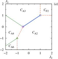
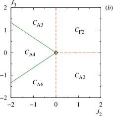
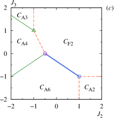
Figure 1: Magnetic phase diagram of the ground state of the Ising chain with the exchange interactions of spins at the sites of the linear chain of the first, second, and third neighbors with (a) antiferromagnetic ($J_{1}=-1$), (b) missing ($J_{1}=0$) and (c) ferromagnetic ($J_{1}=+1$) interactions between the spins at the sites of nearest neighbors

Note that the structure of the magnetic phase diagram (see Fig. 1a and 1c) is antisymmetric with respect to the replacement

$$\{J_{1},J_{3}\}\Leftrightarrow\{-J_{1},-J_{3}\},$$ (26)

which, upon further analysis of the model, allows one to consider the behavior of thermodynamic quantities with only one sign of the parameter of the exchange interaction between spins at the sites of the nearest neighbors and at the same time fully describe the thermodynamics of the system.

In the magnetic phase diagram, with the antiferromagnetic spin exchange parameter at the sites of the second neighbors ($J_{2}<0$) at zero temperature, a point is formed at the following ratios of the model parameters

$$J_{2}=-|J_{1}|/2,\quad J_{3}=0,$$ (27)

which delimits three regions of spin configurations $C_{\text{A}4}$, $C_{\text{A}3}$ and $C_{\text{A}2}$ for the antiferromagnetic parameter of the exchange interaction between the spins at the sites of the first neighbors ($J_{1}<0$), or the regions of $C_{\text{A}4}$, $C_{\text{A}6}$ and $C_{\text{F}2}$ with the ferromagnetic parameter ($J_{1}>0$). This triple point (27) in the phase diagram (Fig. 1) is marked by a circlet and has the ground state energy equal to $E=-|J_{1}|/2$.

In the case of a zero value of the spin exchange parameter at the sites of the first neighbors ($J_{1}=0$), the triple point in the phase diagram (27) shifts to the position where the values of all exchange parameters are zero,

$$J_{1}=J_{2}=J_{3}=0.$$ (28)

This point in the magnetic phase diagram (Fig. 1b) is indicated by a rhombus, it is already common for the five spin configuration regions of $C_{\text{A}2}$, $C_{\text{A}6}$, $C_{\text{A}4}$, $C_{\text{A}3}$, and $C_{\text{F}2}$, and has the energy equal to zero, $E=0$.

Note that this fact does not contradict the Gibbs phase rule, since the considered spin system at a given point (28) is defined as an Ising paramagnet in an absolutely frustrated state (Zarubin et al., 2019a).

Depending on the signs of the parameters of the exchange interactions of spins at the sites of the first and third neighbors at the point (27), the following boundaries of the regions of spin configurations are formed.

In the antiferro-antiferro-antiferromagnetic variant of the parameters of the exchange interactions between the spins at the sites of the nearest, second and third neighbors ($J_{1}<0$, $J_{2}<0$, $J_{3}<0$) and with an increase of the parameter $|J_{3}|$, in the phase diagram from the point (27) a linear segment is formed

$$J_{3}=-J_{1}+2J_{2},\quad J_{1}<J_{2}<J_{1}/2,\quad J_{1}<J_{3}<0,$$ (29)

defining the common boundary of the configuration regions $C_{\text{A}4}$ and $C_{\text{A}2}$, which has the energy $E=J_{2}$.

Also, with an increase of the parameter $|J_{3}|$, and in the ferro-antiferro-ferromagnetic variant of the exchange interaction parameters ($J_{1}>0$, $J_{2}<0$, $J_{3}>0$), from the point (27) a line segment is formed

$$J_{3}=-J_{1}-2J_{2},\quad-J_{1}<J_{2}<-J_{1}/2,\quad 0<J_{3}<J_{1},$$ (30)

defining the boundary of the configuration regions $C_{\text{A}4}$ and $C_{\text{F}2}$, which has an energy $E=J_{2}$.

The considered segments of the boundaries of the phase diagram (29) and (30) start at the point (27), and with a further increase of the parameter $|J_{3}|$ end in position

$$J_{2}=-|J_{1}|,\quad J_{3}=J_{1},$$ (31)

in which there arises another spin configuration $C_{\text{A}6}$ with the antiferromagnetic parameter of the exchange interaction between the spins at the sites of the first neighbors ($J_{1}<0$) or the configuration $C_{\text{A}3}$ with the ferromagnetic parameter ($J_{1}>0$). The triple point (31) in the phase diagram (Fig. 1) is marked by a triangle and has the energy $E=-|J_{1}|$.

With a further increase of the parameter $|J_{3}|$ in the phase diagram at the point (31) the boundaries of already three regions of spin configurations are formed.

Thus, in the antiferro-antiferro-antiferromagnetic variant of the parameters of the exchange interactions between the spins at the sites of the nearest, second, and third neighbors ($J_{1}<0$, $J_{2}<0$, $J_{3}<0$), the lines emerging from the point (31) defining the boundaries of the spin configurations $C_{\text{A}4}$, $C_{\text{A}6}$ and $C_{\text{A}2}$ are given by

$$J_{3}=\frac{J_{1}+2J_{2}}{3},\quad J_{2}\leqslant J_{1},\quad J_{3}\leqslant J_{1},$$ (32)

for regions $C_{\text{A}4}$ and $C_{\text{A}6}$ with the energy of states at the boundary $E=J_{2}$, and also

$$J_{2}=J_{1},\quad J_{3}<-|J_{1}|$$ (33)

for the boundary between the configurations $C_{\text{A}6}$ and $C_{\text{A}2}$ with the energy $E=J_{3}$.

In the ferro-antiferro-ferromagnetic variant of the exchange interaction parameters ($J_{1}>0$, $J_{2}<0$, $J_{3}>0$), the lines emerging from the point (31) defining the boundaries of the spin configurations $C_{\text{A}4}$, $C_{\text{A}3}$ and $C_{\text{F}2}$ are given by the expressions

$$J_{3}=\frac{J_{1}-2J_{2}}{3},\quad J_{2}<J_{1}/2,$$ (34)

$$J_{2}=-J_{1},\quad J_{3}>|J_{1}|,$$ (35)

and the energies of states on these lines are respectively equal to $E=J_{2}$ and $E=-J_{3}$.

On the other hand, in the antiferro-antiferro-ferromagnetic variant of the exchange interaction parameters ($J_{1}<0$, $J_{2}<0$, $J_{3}>0$) with increasing parameter $|J_{3}|$ at the point (27) in the phase diagram the segments

$$J_{3}=\frac{J_{1}-2J_{2}}{3},\quad J_{2}\leqslant-J_{1},\quad J_{3}\geqslant J_{1},$$ (36)

are formed, defining the corresponding boundaries of the configuration regions $C_{\text{A}4}$ and $C_{\text{A}3}$ with the ground state energy equal to $E=J_{2}$, and also the segments

$$J_{3}=-\frac{J_{1}-2J_{2}}{3},\quad J_{1}/2<J_{2}\leqslant-J_{1},\quad 0<J_{3}\leqslant-J_{1},$$ (37)

are formed, defining the boundaries of the configuration regions $C_{\text{A}3}$ and $C_{\text{A}2}$ with the energy

$$E=\frac{J_{1}-J_{3}}{2}.$$ (38)

In the ferro-antiferro-antiferromagnetic variant of the exchange interaction parameters ($J_{1}>0$, $J_{2}<0$, $J_{3}<0$), the boundaries are formed at the point (27), which are described by the expressions

$$J_{3}=\frac{J_{1}+2J_{2}}{3},\quad J_{2}<-J_{1}/2$$ (39)

for regions of spin configurations $C_{\text{A}4}$ and $C_{\text{A}6}$, and

$$J_{3}=-\frac{J_{1}+2J_{2}}{3},\quad-J_{1}/2<J_{2}\leqslant J_{1},\quad-J_{1}\leqslant J_{3}<0,$$ (40)

for regions $C_{\text{A}6}$ and $C_{\text{F}2}$. The energies of the system at zero temperature on the lines (39) and (40) are respectively equal to $E=J_{2}$ and

$$E=-\frac{J_{1}-J_{3}}{2}.$$

Depending on the sign of the exchange interaction parameters between the spins at the sites of the nearest neighbors, the segments (37) or (40) determine the boundaries in the phase diagram, which, passing through the position

$$J_{2}=0,\quad J_{3}=-J_{1}/3,$$ (41)

connect the point (27) with the point

$$J_{2}=|J_{1}|,\quad J_{3}=-J_{1}.$$ (42)

The triple point (42) in the phase diagram (Fig. 1) is marked by a square and has the energy $E=-|J_{1}|$.

In the antiferro-ferro-ferromagnetic variant of the exchange interaction parameters ($J_{1}<0$, $J_{2}>0$, $J_{3}>0$) and with increasing parameter $|J_{3}|$ at the triple point in the magnetic phase diagram (42), another configuration region $C_{\text{F}2}$ is formed, the boundaries of which with the corresponding regions of the spin configurations $C_{\text{A}3}$ and$C_{\text{A}2}$ are defined by the following linear laws (35) and

$$J_{2}>|J_{1}|,\quad J_{3}=-J_{1}.$$ (43)

The energies of the ground state of the system in the positions (35) and (43) are respectively equal to $E=-J_{3}$ and $E=-J_{2}$.

On the other hand, in the ferro-ferro-antiferromagnetic variant of the exchange interactions parameters ($J_{1}>0$, $J_{2}>0$, $J_{3}<0$) and with increasing parameter $|J_{3}|$ at the triple point in the magnetic phase diagram (42), another configuration region $C_{\text{A}2}$ is formed, the boundaries of which with the corresponding regions of the spin configurations $C_{\text{A}6}$ and $C_{\text{F}2}$ are determined by the linear laws (33) and (43) with the corresponding energies $E=J_{3}$ and $E=-J_{2}$.

Note that in the case of zero exchange interaction between the spins at the sites of the nearest neighbors ($J_{1}=0$), the above segments of the boundary between the configurations $C_{\text{A}4}$ and $C_{\text{F}2}$ (29); $C_{\text{A}4}$ and $C_{\text{F}2}$ (30), as well as $C_{\text{A}3}$ and $C_{\text{F}2}$ (37); $C_{\text{A}6}$ and $C_{\text{F}2}$ (40) are absent, i.e. all the triple points described above are combined where the quintuple point is formed, as one can see in Fig. 1b.

Thus, the lines in the magnetic phase diagram of the ground state demonstrate the boundaries of the regions of spin configurations on which a qualitative change in the structure of magnetic ordering of the ground state occurs.

In Fig. 1 dashed lines indicate the boundaries (determined by the following relations of the model parameters (43), (35), (29) and (33) with the antiferromagnetic parameter of the exchange interaction between the spins at the sites of the first neighbors ($J_{1}<0$), as well as (43), (33), (30) and (35) with the ferromagnetic exchange interaction parameter ($J_{1}>0$)), on which the rearrangement of the ground state ordering occurs, and the number of configurations of the system with minimum energy is equal to the sum of the configurations of the regions adjacent to the boundary.

The solid lines in Fig. 1 indicate the boundaries (determined by the following relations of the model parameters (32), (34) and (37) with the antiferromagnetic parameter ($J_{1}<0$), as well as (34), (32) and (40) with the ferromagnetic parameter ($J_{1}>0$)), on which the number of configurations of the system with the minimum energy is greater than the sum of the configurations of the adjacent regions of the phase diagram.

Such a multitude of spin configurations of the system at zero temperature is associated with the rearrangement of the magnetic structure and the appearance at the given phase a point (in the thermodynamic limit) of an infinite number of spin configurations, including a violation of translational invariance.

This situation can be demonstrated by the following example. Note that in the phase diagram shown in Fig. 1a, the boundary indicated by the solid line (37), with the energy (38]) corresponds to the adjacent regions of the spin configurations $C_{\text{A}2}$ and $C_{\text{A}3}$ with the corresponding energies (17) and (19). In the antiferro-ferro-ferromagnetic variant of the exchange interaction parameters, there are other configuration sequences, for example,

$$\left\{\begin{array}[]{ccccccccc}\uparrow&\downarrow&\uparrow&\downarrow&\downarrow&\uparrow&\downarrow&\uparrow&\cdots\\ \downarrow&\uparrow&\downarrow&\downarrow&\uparrow&\downarrow&\downarrow&\uparrow&\cdots\end{array}\right\},$$

with the same energy

$$E_{\text{A}x}=\frac{J_{1}-J_{3}}{2}$$ (44)

or

$$\left\{\begin{array}[]{ccccccccccccc}\uparrow&\uparrow&\downarrow&\uparrow&\downarrow&\uparrow&\uparrow&\downarrow&\uparrow&\downarrow&\uparrow&\downarrow&\cdots\\ \uparrow&\downarrow&\downarrow&\uparrow&\downarrow&\uparrow&\uparrow&\downarrow&\uparrow&\downarrow&\uparrow&\downarrow&\cdots\\ \downarrow&\uparrow&\downarrow&\uparrow&\uparrow&\downarrow&\uparrow&\uparrow&\downarrow&\uparrow&\downarrow&\uparrow&\cdots\\ \downarrow&\downarrow&\uparrow&\downarrow&\uparrow&\uparrow&\downarrow&\uparrow&\downarrow&\uparrow&\downarrow&\uparrow&\cdots\end{array}\right\}$$

with the energy

$$E_{\text{A}y}=\frac{2J_{1}-J_{2}}{3},$$ (45)

which also have minimal ground state energy only at the phase boundary of the regions under consideration (38), as shown in Fig. 2.

Figure 2: The energies of the ground state of spin configurations depending on the ferromagnetic exchange interaction parameter between spins at the sites of third neighbors ($J_{3}\geqslant 0$) in the magnetic phase space region, where $J_{1}=-1$ and $J_{2}=+1$. The frustration regime in the system occurs at the point $J_{3}=+1$. The solid lines indicate the energies $E_{\text{A}2}$ (17) and $E_{\text{A}3}$ (19), the dashed line indicates $E_{\text{A}x}$ (44), the dotted line indicates $E_{\text{A}y}$ (45), and the thick solid line indicates the minimum energy $E_{0}$ (14)

In the terminology of the works (Fisher and Selke, 1981; Pokrovskii and Uimin, 1982; Selke et al., 1985; Barreto and Yeomans, 1985; Yeomans, 1987, 1988), in the magnetic phase diagram of the ground state (Fig. 1), the triple points described above are called mutiphase points, and solid lines are called mutiphase lines.

IV Residual entropy of the system at zero temperature

In the magnetic phase diagram of the ground state of the model with competing exchange interactions of spins at the sites of the first, second, and third neighbors (Fig. 1) in the regions outside the boundaries of the spin configurations and at the boundaries marked by the dashed lines, the corresponding values of the zero-temperature (residual) entropy are zero,

$$\lim_{T\to 0}S=0,$$ (46)

and at the boundaries indicated by solid lines, the entropy of the ground state is no longer zero,

$$\lim_{T\to 0}S>0.$$ (47)

This result (47) does not contradict the third law of thermodynamics, since the entropy is determined

$$S-S_{0}=\intop_{T_{0}}^{T}\frac{\delta Q}{T}$$ (48)

up to the integration constant $S_{0}\geqslant 0$. This constant is chosen equal to zero ($S_{0}=0$) only in the formulation of the Nernst–Planck theorem for equilibrium systems with nondegenerate ground state (Sommerfeld, 1956).

On the other hand, if the Gibbs entropy of the ground state of the system is greater than zero,

$$S(T=0)=\ln W>0,$$

this suggests that the system experiences degeneracy of the ground state, since the statistical weight characterizing the multiplicity of degeneracy of the system is greater than unity ($W>1$) (Nolting, 2018).

Thus, the state of a system in which the entropy of the ground state is not zero (47) should be called frustrated (Zarubin et al., 2019a).

It should be noted that, in contrast to the situation with a smaller number of interactions in the Ising model (Zarubin et al., 2019a), in the case under consideration there are much more relations of exchange interaction parameters in the system, at which the frustrated system behaves differently.

For example, in the magnetic phase diagram in the absence of exchange between the spins of the chain (28) at the quintuple point marked by rhombus in Fig. 1b, a paramagnetic state is realized, characterized by that all configurations of the system have the same probability and have the same zero energy. The entropy of such a state of the system is equal to the natural logarithm of two,

$$S=\ln 2\approx 0.693,$$ (49)

and is the same at any temperature. From this it is clear that the Ising paramagnet is an absolutely frustrated system (Zarubin et al., 2019a).

With the ratio of the exchange interaction parameters of the model (27) at the triple point marked in the phase diagram (Fig. 1) by a circlet, the entropy at zero temperature is equal to the natural logarithm of the golden ratio,

$$\lim_{T\to 0}S=\ln\frac{1+\sqrt{5}}{2}\approx 0.481.$$ (50)

In the phase diagram (Fig. 1), thick solid lines indicate the boundaries of the regions of spin configurations with the ratios of the exchange parameters (37) and (40), as well as square marks indicate triple points (42), at which the residual entropy is equal to

$$\lim_{T\to 0}S=\ln\left[\frac{1}{3}\left(1+\vartheta_{2}+\frac{1}{\vartheta_{2}}\right)\right]\approx 0.382,$$ (51)

$$\vartheta_{2}=\sqrt[3]{\frac{3^{3}+2+\sqrt{(3^{3}+2^{2})3^{3}}}{2}}.$$

Also, thin solid lines mark the boundaries of the configurations when the ratio of the model parameters (32) and (34), as well as triangular points indicate the triple points (31) in the phase diagram (Fig. 1), at which the residual entropy has the following value

$$\lim_{T\to 0}S=\ln\left[\frac{1}{3}\left(\vartheta_{3}+\frac{3}{\vartheta_{3}}\right)\right]\approx 0.281,$$ (52)

$$\vartheta_{3}=\sqrt[3]{\frac{3^{3}+\sqrt{(3^{3}-2^{2})3^{3}}}{2}}.$$

Note that the positions of the frustration of the system in the phase diagram correspond to multiphase points and lines in (Barreto and Yeomans, 1985; Selke et al., 1985).

It should be noted, that the expressions presented above for zero-temperature entropy can be written as

$$S=\ln x_{\text{max}},$$

where the argument of the natural logarithm is the statistical weight of the system, which is defined as the maximum real root of the corresponding equation. Thus for residual entropy (50) this equation has the form

$$x^{2}-x-1=0,$$

for (51) is

$$x^{3}-x^{2}-1=0,$$

and for entropy (52) this equation is

$$x^{3}-x-1=0.$$

For the presented equations, there always exists a single positive real root.

V Thermodynamics of the system in the frustration regime and its vicinity

The thermodynamic functions of the model demonstrate a complicated temperature behavior at various ratios of the parameters of the exchange interaction of spins at the sites of the first, second, and third neighbors.

At zero temperature, the entropy of the Ising chain has either a zero value (46) or a finite value in the frustration regime, with values (49), (50), (51) or (52), as well as at an infinitely high temperature (for any values of the exchange parameters of the model), the entropy of the system is equal to the natural logarithm of two,

$$\lim_{T\to\infty}S=\ln 2,$$ (53)

where the statistical weight of the system ($W=2$) corresponds to the number of states at the site in the model.

Thus, when the temperature changes, the entropy of the system has values in the range

$$0\leqslant S\leqslant\ln 2.$$

Figure 3 shows the entropy behavior of the model outside the frustration regime (line 1), in the frustration regime (lines 2, 3, 4), as well as in the completely frustrated system regime (line 5). At an infinitely high temperature and any values of the exchange interaction parameters of the system, the entropy tends to a finite value equal to (53).

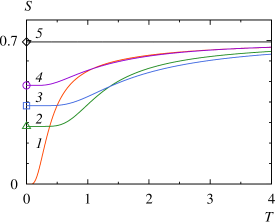
Figure 3: The temperature dependence of the entropy (8) of the Ising chain at five points in the magnetic phase space, where the ratios of the parameters of the exchange interactions of spins are ($J_{1}=-1$, $J_{2}=-0.7$, $J_{3}=-0.4$) for line 1, ($J_{1}=J_{2}=J_{3}=-1$) for line 2, ($J_{1}=-J_{2}=-J_{3}=-1$) for 3, ($J_{1}=-1$, $J_{2}=-1/2$, $J_{3}=0$) for 4, and ($J_{1}=J_{2}=J_{3}=0$) for 5

In turn, the heat capacity of the system is zero for any ratio of the exchange parameters of the spins, and at zero and infinitely high temperatures,

$$\lim_{T\to 0}C=0,\quad\lim_{T\to\infty}C=0.$$ (54)

At intermediate temperatures, the heat capacity has a maximum, which splits into several peaks in the vicinity of the frustration point. For various ratios of the model parameters, several types (scenarios) of the behavior of the temperature evolution of heat capacity are formed.

For example, in the case of the antiferro-antiferro-antiferromagnetic variant of the exchange interaction parameters of the model ($J_{1}<0$, $J_{2}<0$, $J_{3}<0$) with the ratio of the quantities $J_{2}\leqslant J_{1}$ and $J_{3}\leqslant J_{1}$, frustration occurs in the system at a certain ratio of the model parameters (31), therefore, only in this case, the residual entropy is not equal to zero (52), and for all other ratios of the parameters in this interval of values, the entropy of the ground state is zero (46), as shown in Fig. 4. The temperature dependence of entropy at the point of frustration (31) and its small vicinity is presented in more detail in Fig. 5.

In the considered range of model parameters, the temperature dependence of the heat capacity of the system far from the frustration position (31) has one broad maximum, and when approaching the frustration point, this peak splits and an additional sharp peak forms at low temperatures, as shown in Fig. 6. In the vicinity of the frustration regime, the sharp peak (increasing in amplitude and decreasing in width) disappears in full at the frustration point, where only one broad maximum remains (see Fig. 7) (Zarubin et al., 2019b).

Figure 4: The temperature evolution of the entropy (8) of the Ising chain in the antiferro-antiferro-antiferromagnetic variant of the parameters of the exchange interactions of spins, where $J_{1}=J_{2}=-1$, and $J_{3}<0$

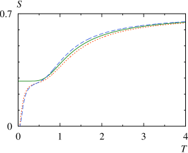
Figure 5: The temperature dependence of the entropy (8) of the Ising chain in the vicinity of the frustration point (31) of the system, where the parameters of the exchange interactions of spins are equal to $J_{1}=J_{2}=-1$, and the values of $J_{3}=\{-1.1,-1,-0.9\}$ correspond to the dotted, solid, and dashed lines

Figure 6: The temperature evolution of the heat capacity (9) of the Ising chain in the antiferro-antiferro-antiferromagnetic variant of the parameters of the exchange interactions of spins, where $J_{1}=J_{2}=-1$, and $J_{3}<0$

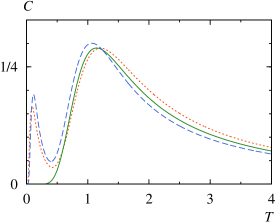
Figure 7: The temperature evolution of the heat capacity (9) of the Ising chain in the vicinity of the frustration point (31) of the system, where the parameters of the exchange interactions of spins are $J_{1}=J_{2}=-1$, and the values of $J_{3}=\{-1.1,-1,-0.9\}$ correspond to the dotted, solid, and dashed lines

Thus, the first scenario of the temperature evolution of the heat capacity peaks in the frustration regime in the system is realized.

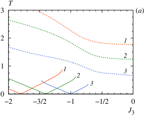
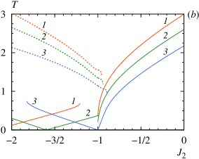
Figure 8: The temperature dependence of the positions of the peaks of the heat capacity (9) of the Ising chain in the antiferro-antiferro-antiferromagnetic variant of the parameters of the exchange interactions of spins ($J_{1}=-1$, $J_{2}<0$, $J_{3}<0$) at the ratio of quantities ($J_{2}\leqslant J_{1}$ and $J_{3}\leqslant J_{1}$), where the numbering of the lines corresponds to the sequential order of values of parameters, where $J_{2}=\{-2.2,-1.6,-1\}$ for the upper (a), and $J_{3}=\{-1.8,-1.4,-1\}$ for the lower (b) graphs

Figure 9: The temperature evolution of the entropy (a) and heat capacity (b) of the Ising chain in the antiferro-antiferro-antiferromagnetic variant of the parameters of the exchange interactions of spins, where $J_{1}=-1$, $J_{2}<0$, and $J_{3}=-1.4$

The evolution of the positions of the heat capacity peaks versus temperature in the range of model parameters (32) for several values of the exchange interaction parameters is shown in Fig. 8. The behavior of the low-temperature peak in this figure is indicated by a solid line, and the evolution of the peak formed at somewhat higher temperatures is shown by a dashed line.

The most distinctly the first scenario of the temperature behavior of the heat capacity peaks is shown in Fig. 8a.

Note that in Fig. 8b a more complicated behavior of the heat capacity peaks was demonstrated, since in the considered range of exchange interaction parameter values, the rearrangement of the ordering of the spin configuration of the ground state occurs twice (for the ratios of the model parameters (32) and (33)). In the first case (32), the system experiences frustrations at spin ordering rearrangement, and in the second case (33) there are no frustrations (see Fig. 9a).

The temperature evolution of entropy and heat capacity is shown in Fig. 9 for the model parameters corresponding to line 2 in Fig. 8b. It can be seen in Fig. 9a that the zero-temperature entropy at the boundary of spin configurations (32) at the frustration point is not zero, but at the boundary (33) at the point where frustration does not occur, the residual entropy is zero.

Figure 9b shows that the temperature function of the heat capacity of the system at the phase separation boundary (32), on which frustration occurs, always has one maximum, and when deviating from these boundaries, the heat capacity behavior noticeably changes, forming a second peak. At the boundary (33), at which frustration of the system does not occur, the temperature evolution of the heat capacity has a more complicated behavior, which will be discussed later.

In the case of the antiferro-antiferro-ferromagnetic variant of the exchange interaction parameters of the model ($J_{1}<0$, $J_{2}<0$, $J_{3}>0$) with the ratio of the quantities ($J_{2}<J_{1}/2$), the system has frustrations at certain ratio of the model parameters (34) with a non-zero value of the residual entropy equal to (52). In this range of exchange interaction parameter values, the temperature evolution of entropy and heat capacity is qualitatively similar to the first scenario described above.

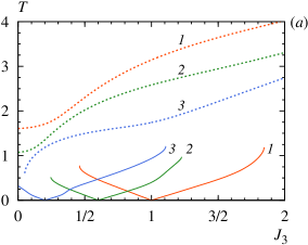
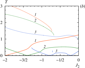
Figure 10: The temperature dependence of the positions of the peaks of the heat capacity (9) of the Ising chain in the antiferro-antiferro-ferromagnetic variant of the parameters of the exchange interactions of spins ($J_{1}=-1$, $J_{2}<0$, $J_{3}>0$) for the ratio of quantities ($J_{2}<J_{1}/2$), where the numbering of the lines corresponds to the sequential values of parameter $J_{2}=\{-2,-1.4,-0.8\}$ for the upper (a), and $J_{3}=\{+1,+0.6,+0.2\}$ for the lower (b) graphs

Figure 11: The temperature evolution of the entropy (a) and heat capacity (b) of the Ising chain in the antiferro-antiferro-ferromagnetic variant of the parameters of the exchange interactions of spins, where $J_{1}=-1$, $J_{2}<0$, and $J_{3}=+0.2$

The temperature evolution of the positions of the heat capacity peaks is shown in Fig. 10. As can be seen from the heat capacity behavior in Fig. 8a and 10a the positions evolution is qualitatively similar.

It should be noted that Fig. 10b shows a complicated evolution of the positions of the heat capacity peaks, which is associated with the existence of two relations of the model parameters in the range of their values at which the system experiences frustrations, (34) and (37).

This situation is demonstrated by the temperature dependences of entropy and heat capacity in Fig. 11, which correspond to line 3 in Fig. 10b.

The residual entropy at the boundaries of spin configurations (34) and (37) at the frustration points is not equal to zero, as can be seen in Fig. 11a.

Figure 11b shows that the temperature dependence of the heat capacity of the system at the phase separation boundaries (34) and (37), on which frustrations arise, always has only one maximum, and when deviating from these boundaries, the heat capacity behavior changes, forming another peak in the vicinity of the boundary.

The second scenario of the formation of the temperature dependence of the heat capacity of the system occurs in the antiferro-antiferro-ferromagnetic variant of the exchange interaction parameters of the model ($J_{1}<0$, $J_{2}<0$, $J_{3}>0$). The frustrations exist in the considered interval of values of the variables of the model.

At first, frustrations arise at a point corresponding to the ratio of the exchange interaction parameters of the model ($J_{2}=J_{1}/2$ and $J_{3}=0$), at which the value of residual entropy is greater than zero and equal to the value (50).

Secondly, frustrations exist in the range of exchange interaction parameters ($J_{1}/2<J_{2}\leqslant 0$ and $0<J_{3}\leqslant-J_{1}/3$) on the phase separation boundary determined by the ratio (37), while the residual entropy is equal to the value (51).

In this case, in the range of model parameters ($J_{1}/2\leqslant J_{2}\leqslant 0$ and $0\leqslant J_{3}\leqslant-J_{1}/3$), the temperature behavior of the heat capacity peaks in the vicinity of the system frustration regime is different from the first scenario described earlier. In this case, far from the frustration regime, the temperature dependence of the heat capacity has only one maximum, and when approaching the frustration point, this peak splits into sharp and broad maxima, and a broad maximum appears and forms already. Also, when approaching the frustration point, these heat capacity maxima diverge and the sharp peak disappears at the frustration point, and when moving away from this point the broad maximum disappears.

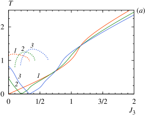
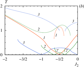
Figure 12: The temperature dependence of the positions of the peaks of the heat capacity (9) of the Ising chain in the antiferro-antiferro-ferromagnetic variant of the parameters of the exchange interactions of spins ($J_{1}=-1$, $J_{2}<0$, $J_{3}>0$) for the ratio of quantities ($J_{1}/2<J_{2}\leqslant 0$ and $0<J_{3}\leqslant-J_{1}/3$), where the numbering of the lines corresponds to the sequential values of parameter $J_{2}=\{-0.5,-0.2,0\}$ for the upper (a), and $J_{3}=\{0,+0.1,+1/3\}$ for the lower (b) graphs

The second scenario of the formation and behavior of the temperature evolution of the peaks of the heat capacity of the system considered here is shown in Fig. 12.

Figure 12b shows a more complicated behavior of the positions of the heat capacity peaks, which is associated with the existence of two relations of the model parameters in this region of their values, for which there are frustrations in the system, (34) and (37). In the considered range of model parameter values, the temperature dependences of entropy and heat capacity were already shown in Fig. 11, for line 2 in Fig. 12b.

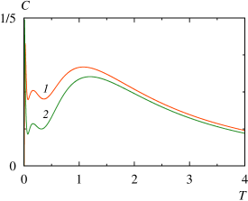
Figure 16: The temperature dependence of the heat capacity of the Ising chain (9) in the vicinity of the frustration points (34) and (37) of the system, where the parameters of the exchange interactions of spins are equal to $J_{1}=-1$, $J_{3}=+0.1$, and the values of $J_{2}=-0.612$ and $J_{2}=-0.365$ correspond to lines 1 and 2 on the graph

It should be noted here that a third peak may appear on the temperature evolution of the heat capacity in the antiferro-antiferro-ferromagnetic variant of the model exchange interaction parameters ($J_{1}<0$, $J_{2}<0$, $J_{3}>0$) in the range from (34) to (37), i.e. near the existence of two frustrated states of the spin system (see lines 2’ in Fig. 12). This small broad maximum arising between the sharp and large broad peaks is shown in Fig. 16.

The third scenario arises in the antiferro-ferro-ferromagnetic variant of the exchange interaction parameters of the model ($J_{1}<0$, $J_{2}>0$, $J_{3}>0$) for the ratios ($0<J_{2}\leqslant-J_{1}$ and $-J_{1}/3<J_{3}\leqslant-J_{1}$). In this range of model parameters with the ratios of exchange interactions (37), the residual entropy is equal to a nonzero value (51), which demonstrates the existence of frustration in the system.

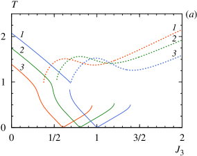
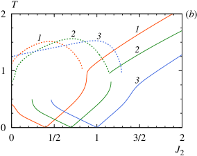
Figure 13: The temperature dependence of the positions of the peaks of the heat capacity (9) of the Ising chain in the antiferro-ferro-ferromagnetic variant of the parameters of the exchange interactions of spins ($J_{1}=-1$, $J_{2}>0$, $J_{3}>0$) for the ratio of quantities ($0<J_{2}\leqslant-J_{1}$ and $-J_{1}/3<J_{3}\leqslant-J_{1}$), where the numbering of the lines corresponds to the sequential values of parameter $J_{2}=\{+0.4,+0.7,+1\}$ for the upper (a), and $J_{3}=\{+0.6,+0.8,+1\}$ for the lower (b) graphs

In this case, the temperature evolution of the heat capacity peaks demonstrates somewhat different behavior from the previously described scenarios. When approaching the position of frustration (37), the peak splits into a broad and sharp peaks, while the sharp peak formed at low temperatures disappears at the point of frustration. When moving away from the frustration point towards small values of the exchange interaction between the spins at the sites of third neighbors ($J_{3}$), the broad peak disappears (see Fig. 13a), and when moving away from this point towards large values of the parameter $J_{3}$, the sharp peak disappears, and only one broad maximum of the function remains. When parameter $J_{2}$ changes (see Fig. 13b), the temperature evolution of the heat capacity peaks is similar to that described earlier, but with inverted behavior.

Obviously, the heat capacity of the system here demonstrates the third scenario of the formation of the temperature evolution of the behavior of the maxima. This behavior is a combination of the two previous scenarios.

This is shown that in Fig. 13 on one side of the frustration point (37) for small values of $J_{3}$ (or large for $J_{2}$) the heat capacity behaves similarly to the second scenario of peak development (see Fig. 12), and for values of $J_{3}$ greater (or less for $J_{2}$) than frustration values (37), the heat capacity behaves already as in the case of the first scenario (see Fig. 10).

Note that the peak splitting described above in three scenarios during the temperature evolution of the magnetic contribution to heat capacity is observed in real rare-earth antiferromagnets (Wada et al., 1995; Berton et al., 1985; Avila et al., 2004; Goruganti et al., 2008; Chang et al., 2010; Romero et al., 2013; Diep, 2013; Kamikawa et al., 2015; Müller et al., 2015) and actinide compounds (Santini et al., 1999), as well as a number of organometallic coordination polymers (Tran and Światek Tran, 2008; Rams et al., 2017), molecular (Fu et al., 2010) and quasi-one-dimensional frustrated (Ahmed et al., 2015) magnets.

It is important to note that the magnetic phase diagram of the ground state also contains the boundaries of the regions of spin configurations on which frustration does not occur (dashed lines in Fig. 1). In such cases, the entropy of the ground state of the system is zero (46), but the rearrangement of the configurations still leads to a change in the behavior of the temperature dependence of the heat capacity peaks of the system, which is quite different from that described above.

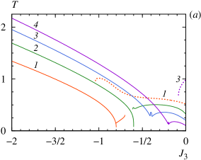
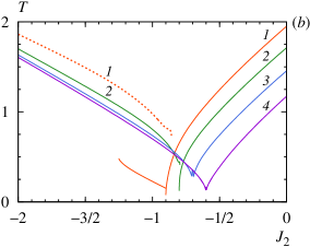
Figure 14: The temperature dependence of the positions of the peaks of the heat capacity (9) of the Ising chain in the antiferro-antiferro-antiferromagnetic variant of the parameters of the exchange interactions of spins ($J_{1}=-1$, $J_{2}<0$, $J_{3}<0$) for the ratio of quantities ($J_{1}<J_{2}<J_{1}/2$ and $J_{1}<J_{3}<0$), where the numbering of the lines corresponds to the sequential values of parameter $J_{2}=\{-0.9,-0.8,-0.7,-0.6\}$ for the upper (a), and $J_{3}=\{-0.8,-0.6,-0.4,-0.2\}$ for the lower (b) graphs

These situations are observed in the magnetic phase diagram in several cases. Firstly, in the antiferro-antiferro-antiferromagnetic variant of the exchange interaction parameters of the model ($J_{1}<0$, $J_{2}<0$, $J_{3}<0$) for the ratio of quantities ($J_{1}<J_{2}<J_{1}/2$ and $J_{1}<J_{3}<0$) at the boundary of the regions of spin configurations (29), as well as for the ratio of quantities ($J_{2}=J_{1}$ and $J_{3}<-|J_{1}|$) on the boundary (33). The behavior of the heat capacity peaks is shown in Fig. 14 and 8.

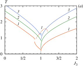
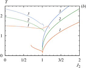
Figure 15: The temperature dependence of the positions of the peaks of the heat capacity (9) of the Ising chain in the antiferro-ferro-ferromagnetic variant of the parameters of the exchange interactions of spins ($J_{1}=-1$, $J_{2}>0$, $J_{3}>0$) for the ratio of quantities ($J_{2}>-J_{1}$ and $J_{3}>-J_{1}$), where the numbering of the lines corresponds to the sequential values of parameter $J_{2}=\{+1.2,+1.6,+2\}$ for the upper (a), and $J_{3}=\{+1.2,+1.6,+2\}$ for the lower (b) graphs

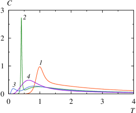
Figure 17: The temperature evolution of the heat capacity (9) of the Ising chain near the magnetic phase boundary, where the ratios of the parameters of the exchange interactions of spins are $J_{1}=-1$ and $J_{2}=-0.9$, and the line numbering corresponds to the sequential values of the parameter $J_{3}=\{-1.5,-0.9,-0.8,-0.5\}$

Secondly, frustrations are absent in the antiferro-ferro-ferromagnetic variant of the exchange interaction parameters of the model ($J_{1}<0$, $J_{2}>0$, $J_{3}>0$) for the ratio of quantities ($J_{2}>-J_{1}$ and $J_{3}>-J_{1}$) at the boundaries of the configuration regions of the ground state (43) and (35). The behavior of the heat capacity peaks is shown in Fig. 15.

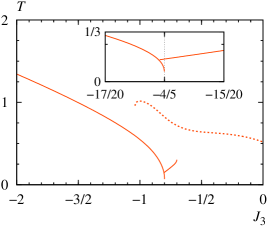
Figure 18: The temperature dependence of the positions of the peaks of the heat capacity (9) of the Ising chain in the antiferro-ferro-ferromagnetic variant of the parameters of the exchange interactions of spins ($J_{1}=-1$, $J_{2}>0$, $J_{3}>0$) near the magnetic phase boundary $C_{\text{A}4}$–$C_{\text{A}2}$ (see Fig. 1a), where the ratio of the parameters of the exchange interactions of spins are $J_{1}=-1$, $J_{2}=-0.9$, and $J_{3}<0$

Figure 19: The temperature evolution of the heat capacity (9) of the Ising chain in the antiferro-antiferro-antiferromagnetic variant of the parameters of the exchange interactions of spins, where $J_{1}=-1$, $J_{2}=-0.9$, and $J_{3}<0$

In the cases presented (with the ratio of the exchange interaction parameters corresponding to the separation boundaries of the configurations of the ground state considered), the position of the maximum temperature dependence of the heat capacity formed at low temperatures does not reach zero temperatures and does not vanished, and the heat capacity peaks are large and small the values of the exchange interaction parameter do not converge at one point on the phase boundary at zero temperature (line 3 in Fig. 17). This behavior of the heat capacity peaks at low temperatures demonstrates the possibility of the formation of metastable states (see the inset in Fig. 18).

In the indicated ranges of the parameters of the exchange interaction of spins at the lattice sites in the vicinity of the interphase boundary and near the point of frustration of the system, it is possible to split the maximum and form a two-peak structure of the temperature dependence of the heat capacity, which differs from the heat capacity structure near the frustration regime, as shown in Fig. 19.

This situation is possible due to the fact that the second (broad) peak has a extension when the ratio of exchange interaction parameters near the frustration point changes, as can be seen from Fig. 8. In this case, the sharp peak in heat capacity can be quite high and narrow at low temperatures and with a ratio of exchange interaction parameters near the separation boundary of the configuration regions (line 2 in Fig. 17).

In the end, it should be noted that in the antiferro-ferro-antiferromagnetic variant of the exchange interaction parameters of the model ($J_{1}<0$, $J_{2}>0$, $J_{3}<0$), the situation of competition between the exchange interactions of the model does not appear and therefore changes in the ordering of the spin configuration are not formed. The entropy of the ground state is always zero, and the heat capacity of such a system has only one broad peak.

VI Conclusions

In this work, the exact analytic expressions for the entropy and heat capacity of the one-dimensional Ising model are obtained using the Kramers–Wannier transfer matrix method taking into account the exchange interactions of spins at the sites of the first, second, and third neighbors. Based in the magnetic phase diagram of the model, the analysis of configurational features of the ground state and frustration properties of the system is carried out.

Criteria are formulated and relationships of model parameters are determined for which magnetic frustrations arise in the considered one-dimensional spin systems. It was found out that the frustrations are caused by competition between the energies of the exchange interactions of spins. Thus, it was shown that in the frustration regime the system undergoes a rearrangement of the magnetic ordering structure of the ground state, which begins to include many spin configurations comparable to the size of the system, including the absence of translational invariance.

The characteristic behavior of the entropy and heat capacity of the system in the regime of frustration and near it is analyzed, a cardinal difference in the behavior of the magnetic system in the frustration region and outside it is shown.

It has been determined that the most important evidence of the existence of magnetic frustrations in the system is the nonzero value of the residual entropy in this regime, and this property does not contradict the third law of thermodynamics. It is also shown that the residual entropy can have the same nonzero value for entire intervals of model parameter values.

It was found that one of the common features of frustrated systems is the effect of peak splitting on the temperature evolution of the magnetic contribution of the heat capacity in the immediate vicinity of the frustration regime, which can be observed in real antiferromagnets based on rare-earth metals and actinide compounds, as well as a number of organometallic coordination polymers, molecular and quasi-one-dimensional frustrated magnets.

Differences in the formation of the structure of the temperature evolution of the heat capacity are revealed, which demonstrate three scenarios in the behavior of the heat capacity peaks in the frustration region of the system for various values of the ratios of the exchange interaction parameters of the model.

The most important difference in the temperature dependence of the heat capacity in the region of frustration and outside it lies in the specific features of the behavior of the heat capacity peak at low temperatures with the ratio of the model parameters corresponding to the boundaries of the spin configurations. In the cases under consideration, out of frustration regime the indicated heat capacity peak does not reach zero temperatures and does not disappear at the separation boundary of spin configurations. This peak can have a large hight, which distinguishes it from the corresponding peaks of heat capacity in the region of existence of system frustrations.

It is shown in the work that the heat capacity of the system near the boundary of the phase diagram outside the frustration region demonstrates a transition to the metastable state.

Thus, the proposed analysis scheme allows us to consider a wide range of phenomena in one-dimensional (or quasi-one-dimensional) magnetic systems with frustrations and to describe their relationship with the features of thermodynamic functions. The mathematical apparatus developed in the work makes it possible to solve similar problems in more complicated models of statistical physics, in particular, in multicomponent spin models with discrete symmetry and an arbitrary spin value.

References

- Kassan-Ogly and Filippov (2010) F. A. Kassan-Ogly and B. N. Filippov, Bull. Russ. Acad. Sci. Phys. 74, 1452 (2010).
- Normand (2009) B. Normand, Contemp. Phys. 50, 533 (2009).
- Balents (2010) L. Balents, Nature 464, 199 (2010).
- Lacroix et al. (2011) C. Lacroix, P. Mendels, and F. Mila, eds., Introduction to frustrated magnetism: Materials, experiments, theory (Springer, Berlin, Heidelberg, 2011).
- Sadoc and Mosseri (1999) J.-F. Sadoc and R. Mosseri, Geometrical frustration (Cambridge University Press, New York, 1999).
- Kudasov et al. (2012) Y. B. Kudasov, A. S. Korshunov, V. N. Pavlov, and D. A. Maslov, Phys. Usp. 55, 1169 (2012).
- Diep (2013) H. T. Diep, ed., Frustrated spin systems, 2nd ed. (World Scientific, New Jersey, 2013).
- Vasiliev et al. (2018) A. N. Vasiliev, O. S. Volkova, E. A. Zvereva, and M. M. Markina, Low dimensional magnetism (Fizmatlit, Moscow, 2018) [in Russian].
- Toulouse (1977) G. Toulouse, Commun. Phys. 2, 115 (1977).
- Vannimenus and Toulouse (1977) J. Vannimenus and G. Toulouse, J. Phys. C: Solid State Phys. 10, L537 (1977).
- Baxter (1982) R. J. Baxter, Exactly solved models in statistical mechanics (Academic Press, London, 1982).
- Ising (1925) E. Ising, Z. Physik 31, 253 (1925).
- Brush (1967) S. G. Brush, Rev. Mod. Phys. 39, 883 (1967).
- Niss (2005) M. Niss, Arch. Hist. Exact Sci. 59, 267 (2005).
- Newell and Montroll (1953) G. F. Newell and E. W. Montroll, Rev. Mod. Phys. 25, 353 (1953).
- Kassan-Ogly (2001) F. A. Kassan-Ogly, Phase Transitions 74, 353 (2001).
- Kassan-Ogly et al. (1989) F. A. Kassan-Ogly, E. V. Kormiltsev, V. E. Naish, and I. V. Sagaradze, Sov. Phys. Solid State 31, 43 (1989).
- Zarubin et al. (2016) A. V. Zarubin, F. A. Kassan-Ogly, and A. I. Proshkin, Mater. Sci. Forum 845, 122 (2016).
- Kramers and Wannier (1941) H. A. Kramers and G. H. Wannier, Phys. Rev. 60, 252 (1941).
- Oguchi (1965) T. Oguchi, J. Phys. Soc. Jpn. 20, 2236 (1965).
- Zarubin et al. (2019a) A. V. Zarubin, F. A. Kassan-Ogly, A. I. Proshkin, and A. E. Shestakov, J. Exp. Theor. Phys. 128, 778 (2019a).
- Domb (1960) C. Domb, Adv. Phys. 9, 149 (1960).
- Horn and Johnson (2013) R. A. Horn and C. R. Johnson, Matrix analysis, 2nd ed. (Cambridge University Press, Cambridge, 2013).
- Nolting and Ramakanth (2009) W. Nolting and A. Ramakanth, Quantum theory of magnetism (Springer, Berlin, Heidelberg, 2009).
- Mussardo (2010) G. Mussardo, Statistical field theory: An introduction to exactly solved models in statistical physics (Oxford University Press, Oxford, New York, 2010).
- Gould and Tobochnik (2010) H. Gould and J. Tobochnik, Statistical and thermal physics: With computer applications (Princeton University Press, Princeton, 2010).
- Martínez-Garcilazo et al. (2009) J. P. Martínez-Garcilazo, R. Márquez-Islas, and C. Ramírez-Romero, Rev. mex. fís. E 55, 136 (2009).
- Stephenson (1970) J. Stephenson, Can. J. Phys. 48, 1724 (1970).
- Fisher and Selke (1980) M. E. Fisher and W. Selke, Phys. Rev. Lett. 44, 1502 (1980).
- Fisher and Selke (1981) M. E. Fisher and W. Selke, Phil. Trans. R. Soc. A 302, 1 (1981).
- Selke et al. (1985) W. Selke, M. Barreto, and J. Yeomans, J. Phys. C: Solid State Phys. 18, L393 (1985).
- Selke (1988) W. Selke, Phys. Reports 170, 213 (1988).
- Yeomans (1988) J. Yeomans, “The theory and application of axial Ising models,” in Solid state physics, Vol. 41, edited by H. Ehrenreich and D. Turnbull (Academic Press, San Diego, 1988) pp. 151–200.
- Price (1983) G. D. Price, Phys. Chem. Miner. 10, 77 (1983).
- Barreto and Yeomans (1985) M. Barreto and J. Yeomans, Physica A 134, 84 (1985).
- Pokrovskii and Uimin (1982) V. L. Pokrovskii and G. V. Uimin, Sov. Phys. JETP 55, 950 (1982).
- Yeomans (1987) J. Yeomans, “The application of axial ising models to the description of modulated order,” in Incommensurate crystals, liquid crystals, and quasi-crystals, edited by J. F. Scott and N. A. Clark (Plenum Press, New York, 1987).
- Sommerfeld (1956) A. Sommerfeld, Thermodynamics and statistical mechanics (Academic Press, New York, 1956).
- Nolting (2018) W. Nolting, Theoretical physics 8: Statistical physics (Springer, Cham, 2018).
- Zarubin et al. (2019b) A. V. Zarubin, F. A. Kassan-Ogly, and A. I. Proshkin, J. Phys.: Conf. Ser. 1389, 012009 (2019b).
- Wada et al. (1995) H. Wada, H. Imai, and M. Shiga, J. Alloys Compd. 218, 73 (1995).
- Berton et al. (1985) A. Berton, J. Chaussy, J. Flouquet, J. Odin, J. Peyrard, and F. Holtzberg, Phys. Rev. B 31, 4313 (1985).
- Avila et al. (2004) M. A. Avila, S. L. Bud’ko, and P. C. Canfield, J. Magn. Magn. Mater. 270, 51 (2004).
- Goruganti et al. (2008) V. Goruganti, K. D. D. Rathnayaka, J. H. Ross, Y. Öner, C. S. Lue, and Y. K. Kuo, J. Appl. Phys. 103, 073919 (2008).
- Chang et al. (2010) L. J. Chang, M. Prager, J. Perßon, J. Walter, E. Jansen, Y. Y. Chen, and J. S. Gardner, J. Phys.: Condens. Matter 22, 076003 (2010).
- Romero et al. (2013) M. A. Romero, A. A. Aligia, J. G. Sereni, and G. Nieva, J. Phys.: Condens. Matter 26, 025602 (2013).
- Kamikawa et al. (2015) S. Kamikawa, I. Ishii, Y. Noguchi, H. Goto, T. K. Fujita, F. Nakagawa, H. Tanida, M. Sera, and T. Suzuki, Phys. Procedia 75, 187 (2015).
- Müller et al. (2015) R. A. Müller, A. Desilets-Benoit, N. Gauthier, L. Lapointe, A. D. Bianchi, T. Maris, R. Zahn, R. Beyer, E. Green, J. Wosnitza, Z. Yamani, and M. Kenzelmann, Phys. Rev. B 92, 184432 (2015).
- Santini et al. (1999) P. Santini, R. Lémanski, and P. Erdős, Adv. Phys. 48, 537 (1999).
- Tran and Światek Tran (2008) V. H. Tran and B. Światek Tran, Dalton Trans. , 4860 (2008).
- Rams et al. (2017) M. Rams, Z. Tomkowicz, M. Böhme, W. Plass, S. Suckert, J. Werner, I. Jess, and C. Näther, Phys. Chem. Chem. Phys. 19, 3232 (2017).
- Fu et al. (2010) Z.-D. Fu, P. Kögerler, U. Rücker, Y. Su, R. Mittal, and T. Brückel, New J. Phys. 12, 083044 (2010).
- Ahmed et al. (2015) N. Ahmed, A. A. Tsirlin, and R. Nath, Phys. Rev. B 91, 214413 (2015).