Adaptivity of Stochastic Gradient Methods for Nonconvex Optimization

Abstract

Adaptivity is an important yet under-studied property in modern optimization theory. The gap between the state-of-the-art theory and the current practice is striking in that algorithms with desirable theoretical guarantees typically involve drastically different settings of hyperparameters, such as step-size schemes and batch sizes, in different regimes. Despite the appealing theoretical results, such divisive strategies provide little, if any, insight to practitioners to select algorithms that work broadly without tweaking the hyperparameters. In this work, blending the “geometrization” technique introduced by Lei & Jordan (2016) and the SARAH algorithm of Nguyen et al. (2017), we propose the Geometrized SARAH algorithm for non-convex finite-sum and stochastic optimization. Our algorithm is proved to achieve adaptivity to both the magnitude of the target accuracy and the Polyak-Łojasiewicz (PL) constant, if present. In addition, it achieves the best-available convergence rate for non-PL objectives simultaneously while outperforming existing algorithms for PL objectives.

1 Introduction

We study smooth nonconvex problems of the form

$$\min_{x\in\mathbb{R}^{d}}\left\{f(x)\overset{\triangle}{=}\mathbb{E}{f_{\xi}(x)}\right\}\,,$$ (1)

where the randomness comes from the selection of data points and is represented by the index $\xi$. If the number of indices $n$ is finite, then we talk about empirical risk minimization and $\mathbb{E}{f_{\xi}(x)}$ can be written in the finite-sum form, $\nicefrac{{1}}{{n}}\sum_{i=1}^{n}f_{i}(x)$. If $n$ is not finite or if it is infeasible to process the entire dataset, we are in the online learning setting, where one obtains independent samples of $\xi$ at each step. We assume that an optimal solution $x^{\star}$ of (1) exists and its value is finite: $f(x^{\star})>-\infty$.

1.1 The many faces of stochastic gradient descent

We start with a brief review of relevant aspects of gradient-based optimization algorithms. Since the number of functions $n$ can be large or even infinite, algorithms that process subsamples are essential. The canonical example is Stochastic Gradient Descent (SGD) (Nemirovsky & Yudin, 1983; Nemirovski et al., 2009; Gower et al., 2019), in which updates are based on single data points or small batches of points. The terrain around the basic SGD method has been thoroughly explored in recent years, resulting in theoretical and practical enhancements such as Nesterov acceleration (Allen-Zhu, 2017), Polyak momentum (Polyak, 1964; Sutskever et al., 2013), adaptive step sizes (Duchi et al., 2011; Kingma & Ba, 2014; Reddi et al., 2019; Malitsky & Mishchenko, 2019), distributed optimization (Ma et al., 2017; Alistarh et al., 2017; Stich, 2018), importance sampling (Zhao & Zhang, 2015; Qu et al., 2015), higher-order optimization (Tripuraneni et al., 2018; Kovalev et al., 2019b), and several other useful techniques.

Table 1: Complexity to reach an $\epsilon$-approximate first-order stationary points ($\mathbb{E}{\left\lVert\nabla f(x)\right\rVert^{2}}\leq\epsilon^{2}$ with $L,\sigma^{2},\Delta_{f}=O(1)$).

Method	Complexity	Required knowledge
GD Nesterov (2018)	${\cal O}\left(\frac{n}{\epsilon^{2}}\right)$	$L$
SVRG Reddi et al. (2016)	${\cal O}\left(n+\frac{n^{2/3}}{\epsilon^{2}}\right)$	$L$
SCSG Lei et al. (2017)	$\tilde{{\cal O}}\left(\frac{1}{\epsilon^{10/3}}\wedge\frac{n^{2/3}}{\epsilon^{2}}\right)$	$L$
SNVRG Zhou et al. (2018)	$\tilde{{\cal O}}\left(\frac{1}{\epsilon^{3}}\wedge\frac{\sqrt{n}}{\epsilon^{2}}\right)$	$L,\sigma^{2},\epsilon$
	$\tilde{{\cal O}}\left(n+\frac{\sqrt{n}}{\epsilon^{2}}\right)$	$L$
SARAH Variants Fang et al. (2018)	$\mathcal{O}\left(n+\frac{\sqrt{n}}{\epsilon^{2}}\right)$	$L$
Wang et al. (2018); Nguyen et al. (2019)
Q-Geom-SARAH (Theorem 3)	${\color[rgb]{1,0,0}\tilde{\mathcal{O}}\left(\left\{n^{3/2}+\frac{\sqrt{n}}{\mu}\right\}\wedge\frac{1}{\epsilon^{3}}\wedge\frac{\sqrt{n}}{\epsilon^{2}}\right)}$	$L$
E-Geom-SARAH (Theorem 4)	${\color[rgb]{1,0,0}\tilde{\mathcal{O}}\bigg{(}\left(\frac{1}{\mu\wedge\epsilon}\right)^{2(1+\delta)}\wedge\left\{n+\frac{\sqrt{n}}{\mu}\right\}\wedge\frac{1}{\epsilon^{4}}\wedge\frac{\sqrt{n}}{\epsilon^{2}}\bigg{)}}$	$L$
Non-adaptive Geom-SARAH (Theorem 5)	${\color[rgb]{1,0,0}\mathcal{O}\left(\left\{\frac{1}{\epsilon^{4/3}(\mu\wedge\epsilon)^{2/3}}\wedge n\right\}+\frac{1}{\mu}\left\{\frac{1}{\epsilon^{4/3}(\mu\wedge\epsilon)^{2/3}}\wedge n\right\}^{1/2}\right)}$	$L,\sigma^{2},\epsilon,\mu$

A particularly productive approach to enhancing SGD has been to make use of variance reduction, in which the classical stochastic gradient direction is modified in various ways so as to drive the variance of the gradient estimator towards zero. This significantly improves the convergence rate and may also enhance the quality of the output solution. The first variance-reduction method was SAG (Roux et al., 2012), closely followed by many more, for instance, SDCA (Shalev-Shwartz & Zhang, 2013), SVRG (Johnson & Zhang, 2013), S2GD (Konečný & Richtárik, 2013), SAGA (Defazio et al., 2014a), FINITO (Defazio et al., 2014b), $\epsilon\mathcal{N}$-SAGA (Hofmann et al., 2015), q-SAGA (Hofmann et al., 2015), QUARTZ (Qu et al., 2015), SCSG (Lei et al., 2017), SARAH (Nguyen et al., 2017), S2CD (Konečný et al., 2017), k-SVRG (Raj & Stich, 2018), SNVRG (Zhou et al., 2018), JacSketch (Gower et al., 2018), Spider (Fang et al., 2018), SpiderBoost (Wang et al., 2018), L-SVRG (Kovalev et al., 2019a) and GJS (Hanzely & Richtárik, 2019). A unified analysis of many of these methods can be found in Gorbunov et al. (2020).

1.2 The dilemma of parameter tuning

Formally, each iteration of vanilla and variance-reduced SGD methods can be written in the generic form

$$x^{+}=x-\eta g,$$ (2)

where $x\in\mathbb{R}^{d}$ is the current iterate, $\eta>0$ is a step size and $g\in\mathbb{R}^{d}$ is a stochastic estimator of the true gradient $\nabla f(x)$.

A major drawback of many such methods is their dependence on parameters that are unlikely to be known in a real-world machine-learning setting. For instance, they may require the knowledge of a uniform bound on the variance or second moment of the stochastic estimators of the gradient which is simply not available, and might not even hold in practice. Moreover, some algorithms perform well in either low precision or high precision regimes and in order to make them perform well in all regimes, they require knowledge of extra parameters, such as target accuracy, which may be difficult to tune. Another related issue is the lack of adaptivity of many SGD variants to different modelling regimes. For example, in order to obtain good theoretical and experimental behavior for non-convex $f$, one needs to run a custom variant of the algorithm if the function is known to satisfy some extra assumptions such as the Polyak-Łojasiewicz (PL) inequality. As a consequence, practitioners are often forced to spend valuable time and resources tuning various parameters and hyper-parameters of their methods, which poses serious issues in implementation and practical deployment.

Table 2: Complexity to reach an $\epsilon$-approximate solution ( $\mathbb{E}{f(x)-f(x^{\star})}\leq\epsilon^{2}$ with $L,\sigma^{2},\Delta_{f}=O(1)$).

Method	Complexity	Required Knowledge
SVRG Li & Li (2018)	$\tilde{{\cal O}}\left(n+\frac{n^{2/3}}{\mu}\right)$	$L$
SCSG Lei et al. (2017)	$\tilde{{\cal O}}\left(\left(\frac{1}{\mu\epsilon^{2}}\wedge n\right)+\frac{1}{\mu}\left(\frac{1}{\mu\epsilon^{2}}\wedge n\right)^{2/3}\right)$	$L,\sigma^{2},\epsilon,\mu$
	$\tilde{{\cal O}}\left(n+\frac{n^{2/3}}{\mu}\right)$	$L$
SNVRG Zhou et al. (2018)	$\tilde{{\cal O}}\left(\left(\frac{1}{\mu\epsilon^{2}}\wedge n\right)+\frac{1}{\mu}\left(\frac{1}{\mu\epsilon^{2}}\wedge n\right)^{1/2}\right)$	$L,\sigma^{2},\epsilon,\mu$
	$\tilde{{\cal O}}\left(n+\frac{\sqrt{n}}{\mu}\right)$	$L$
SARAH Variants Wang et al. (2018); Nguyen et al. (2019)	$\tilde{\mathcal{O}}\left(n+\frac{1}{\mu^{2}}\right)$	$L$
Q-Geom-SARAH (Theorem 3)	${\color[rgb]{1,0,0}\tilde{\mathcal{O}}\left(\left(\frac{1}{\mu^{2}\wedge\mu\epsilon^{2}}\right)^{3(1+\delta)/2}\wedge\left\{n^{3/2}+\frac{\sqrt{n}}{\mu}\right\}\right)}$	$L$
E-Geom-SARAH (Theorem 4)	${\color[rgb]{1,0,0}\tilde{\mathcal{O}}\bigg{(}\left(\frac{1}{\mu^{2}\wedge\mu\epsilon^{2}}\right)^{1+\delta}\wedge\left\{n+\frac{\sqrt{n}}{\mu}\right\}\bigg{)}}$	$L$

1.3 The search for adaptive methods

The above considerations motivate us to impose some algorithm design restrictions so as to resolve the aforementioned issues. First of all, good algorithms should be adaptive in the sense that they should perform comparably to methods with tuned parameters without an a-priori knowledge of the optimal parameter settings. In particular, in the non-convex regime, we might wish to design an algorithm that does not invoke nor need any bound on the variance of the stochastic gradient, or any predefined target accuracy in its implementation. In addition, we should desire algorithms which perform well if the Polyak-Lojasiewicz PL constant (or strong convexity parameter) $\mu$ happens to be large and yet are able to converge even if $\mu=0$; all automatically, without the need for the method to be altered by the practitioner.

There have been several works on this topic, originating from works studying asymptotic rate for SGD with stepsize ${\cal O}(t^{-\alpha})$ for $\alpha\in(\nicefrac{{1}}{{2}},1)$ Ruppert (1988); Polyak (1990); Polyak & Juditsky (1992) up to the most recent paper Lei & Jordan (2019) which focuses on convex optimization (e.g. Moulines & Bach, 2011; Bach & Moulines, 2013; Flammarion & Bach, 2015; Dieuleveut et al., 2017; Xu et al., 2017; Levy et al., 2018; Chen et al., 2018; Xu et al., 2019; Vaswani et al., 2019; Lan et al., 2019; Hazan & Kakade, 2019).

This line of research has shown that algorithms with better complexity can be designed in a finite-sum setting with some levels of adaptivity, generally using the previously mentioned technique–variance reduction. Unfortunately, while these algorithms show some signs of adaptivity, e.g., they do not require the knowledge of $\mu$, they usually fail to adapt to more than one regimes at once: strongly-convex vs convex loss functions, non-convex vs gradient-dominated regime and low vs high precision. To the best of our knowledge, the only paper that tackles multiple such issues is the work of Lei & Jordan (2019). However, even this work does not provide full adaptivity as it focuses on the convex setting. We are not aware of any work which manages to provide a fully adaptive algorithm in the non-convex setting.

1.4 Contributions

In this work we present a new method—the geometrized stochastic recursive gradient (Geom-SARAH) algorithm—that exhibits adaptivity to the PL constant, target accuracy and to the variance of stochastic gradients. Geom-SARAH is a double-loop procedure similar to the SVRG or SARAH algorithms. Crucially, our algorithm does not require the computation of the full gradient in the outer loop as performed by other methods, but makes use of stochastic estimates of gradients in both the outer loop and the inner loop. In addition, by exploiting a randomization technique “geometrization” that allows certain terms to telescope across the outer loop and the inner loop, we obtain a significantly simpler analysis. As a byproduct, this allows us to obtain adaptivity, and our rates either match the known lower bounds Fang et al. (2018) or achieve the same rates as existing state-of-the-art specialized methods, perhaps up to a logarithmic factor; see Table 1 and 2 for the comparison of two versions of Geom-SARAH with existing methods. On a side note, we develop a non-adaptive version of Geom-SARAH (the last row of Table 1) that strictly outperforms existing methods in PL settings. Interestingly, when $\epsilon\sim\mu$, our complexity even beats the best available rate for strongly convex functions (Allen-Zhu, 2018).

We would like to point out that our notion of adaptivity is different from the one pursued by algorithms such as AdaGrad Duchi et al. (2011) or Adam Kingma & Ba (2014); Reddi et al. (2019), where they focus on the geometry of the loss surface. In our case, we focus on adaptivity to different parameters and regimes.

2 Preliminaries

2.1 Basic notation and definitions

We use $\left\lVert\cdot\right\rVert$ to denote standard Euclidean norm, we write either $\min\{a,b\}$ (resp. $\max\{a,b\}$) or $a\wedge b$ (resp. $a\vee b$) to denote minimum and maximum, and we use standard big ${\cal O}$ notation to leave out constants. We adopt the computational cost model of the IFO framework introduced by Agarwal & Bottou (2014) in which upon query $x$, the IFO oracle samples $i$ and out outputs the pair $(f_{i}(x),\nabla f_{i}(x))$. A single such query incurs a unit cost.

Assumption 1.

The stochastic gradient of $f$ is $L$-Lipschitz in expectation. That is,

$$\mathbb{E}{\left\lVert\nabla f_{\xi}(x)-\nabla f_{\xi}(y)\right\rVert}\leq L\left\lVert x-y\right\rVert,\quad\forall x,y\in\mathbb{R}^{d}.$$ (3)

Assumption 2.

The stochastic gradient of $f$ has uniformly bounded variance. That is, there exists $\sigma^{2}>0$ such that

$$\mathbb{E}\left\lVert\nabla f_{\xi}(x)-\nabla f(x)\right\rVert^{2}\leq\sigma^{2},\quad\forall x\in\mathbb{R}^{d}.$$ (4)

Assumption 3.

$f$ satisfies the PL condition with parameter $\mu\geq 0$. That is,

$$\left\lVert\nabla f(x)\right\rVert^{2}\geq 2\mu(f(x)-f(x^{\star})),\quad\forall x\in\mathbb{R}^{d},$$ (5)

where $x^{\star}=\arg\min f(x)$.

We denote $\Delta_{f}\overset{\triangle}{=}f(x_{0})-f(x^{\star})$ to be functional distance to optimal solution.

For non-convex objectives, our goal is to output an $\epsilon$-approximate first-order stationary point, which is summarized in the following definition.

Definition 1.

We say that $x\in\mathbb{R}^{d}$ is an $\epsilon$-approximate first-order stationary point of (1) if

$$\left\lVert\nabla f(x)\right\rVert^{2}\leq\epsilon^{2}.$$

For a gradient dominated function, the quantity of the interest is the functional distance from an optimum, characterized in the following definition.

Definition 2.

We say that $x\in\mathbb{R}^{d}$ is an $\epsilon$-accurate solution of (1) if

$$f(x)-f(x^{\star})\leq\epsilon^{2}.$$

2.2 Accuracy independence and almost universality

We review two fundamental definitions introduced by Lei & Jordan (2019) that serve as a building block for desirable “parameter-free” optimization algorithms. We refer to the first property as $\epsilon$-independence.

Definition 3.

An algorithm is $\epsilon$-independent if it guarantees convergence at all target accuracies $\epsilon>0$.

This is a crucial property as the desired target accuracy is usually not known a-priori. Moreover, an $\epsilon$-independent algorithm can provide convergence to any precision without the need for a manual adjustment of the algorithm or its parameters. To illustrate this, we consider Spider Fang et al. (2018) and Spiderboost Wang et al. (2018) algorithms. Both of these enjoy the same complexity ${\cal O}(n+\nicefrac{{\sqrt{n}}}{{\epsilon^{2}}})$ for non-convex smooth functions, but the stepsize for Spider is $\epsilon$-dependent, making it impractical as this value is often hard to tune.

The second property is inspired by the notion of universality (Nesterov, 2015), requiring for an algorithm to not rely on any a-priori knowledge of smoothness or any other parameter such as the bound on variance.

Definition 4.

An algorithm is almost universal if it only requires the knowledge of the smoothness parameter $L$.

There are several algorithms that satisfy both properties for smooth non-convex optimization, including SAGA, SVRG Reddi et al. (2016), Spiderboost Wang et al. (2018), SARAH Nguyen et al. (2017), and SARAH-SGD Tran-Dinh et al. (2019). Unfortunately, these algorithms are not able to provide a good result in both low and high precision regimes, and in order to perform well, they require the knowledge of extra parameters. This is not the case for our algorithm which is both almost universal and $\epsilon$-independent. Moreover, our method is adaptive to the PL constant $\mu$, and to low and high precision regimes.

2.3 Geometric distribution

Finally, we introduce an important technical tool behind the design of our algorithm, the geometric distribution, denoted by $N\sim\mathrm{Geom}(\gamma)$. Recall that

$$\operatorname{Prob}(N=k)=\gamma^{k}(1-\gamma),\forall k=1,2,\dots,$$

where an elementary calculation shows that

$${\rm E}_{\mathrm{Geom}(\gamma)}\left[N\right]=\frac{\gamma}{1-\gamma}.$$

We use the geometric distribution mainly due to its following property, which helps us to significantly simplify the analysis of our algorithm.

Lemma 1.

Let $N\sim\mathrm{Geom}(\gamma)$. Then for any sequence $D_{0},D_{1},\ldots$ with $\mathbb{E}{|D_{N}|}<\infty$,

$$\mathbb{E}{D_{N}-D_{N+1}}=\frac{1}{\mathbb{E}{N}}(D_{0}-\mathbb{E}{D_{N}}).$$ (6)

Remark 1.

The requirement $\mathbb{E}|D_{N}|<\infty$ is essential. A useful sufficient condition is $|D_{k}|=O(\mathrm{Poly}(k))$ because a geometric random variable has finite moments of any order.

3 Algorithm

  Input: stepsizes $\{\eta_{j}\}$, big-batch sizes $\{B_{j}\}$, expected inner-loop queries $\{m_{j}\}$, mini-batch sizes $\{b_{j}\}$, initializer $\tilde{x}_{0}$, tail-randomized fraction $\delta$

  for $j=1,\dots\lceil(1+\delta)T\rceil$ do

     $x^{(j)}_{0}=\tilde{x}_{j-1}$

     Sample $J_{j}$, $|J_{j}|=B_{j}$

     $v^{(j)}_{0}=\frac{1}{B_{j}}\sum_{i\in J_{j}}\nabla f_{i}(x^{(j)}_{0})$

     Sample $N_{j}\sim\text{Geom}(\gamma_{j})$ s.t. $\mathbb{E}{N_{j}}=\nicefrac{{m_{j}}}{{b_{j}}}$

     for $k=0,\dots,N_{j}-1$ do

        $x^{(j)}_{k+1}=x^{(j)}_{k}-\eta_{j}v^{(j)}_{k}$

        Sample $I^{(j)}_{k}$, $|I^{(j)}_{k}|=b_{j}$

        $\displaystyle v^{(j)}_{k+1}=\frac{1}{b_{j}}\sum_{i\in I^{(j)}_{k}}(\nabla f_{i}(x^{(j)}_{k+1})-\nabla f_{i}(x^{(j)}_{k}))+v^{(j)}_{k}$

     end for

  end for

  Generate $\mathcal{R}(T)$ supported on $\{T,\ldots,\lceil(1+\delta)T\rceil\}$ with $\displaystyle\operatorname{Prob}(\mathcal{R}(T)=j)=\nicefrac{{\eta_{j}m_{j}}}{{\sum_{j=T}^{\lceil(1+\delta)T\rceil}\eta_{j}m_{j}}}$

  Output: $\tilde{x}_{\mathcal{R}(T)}$

Algorithm 1 Geom-SARAH

The algorithm that we propose can be seen as a combination of the structure of SCSG methods Lei & Jordan (2016); Lei et al. (2017) and the SARAH biased gradient estimator

$$v^{(j)}_{k+1}=\frac{1}{b_{j}}\sum_{i\in I^{(j)}_{k}}\left(\nabla f_{i}(x^{(j)}_{k+1})-\nabla f_{i}(x^{(j)}_{k})\right)+v^{(j)}_{k}$$

due to its recent success in the non-convex setting. Our algorithm consists of several epochs. In each epoch, we start with an initial point $x^{(j)}_{0}$ from which the gradient estimator is computed using $B_{j}$ sampled indices, which is not necessarily the full gradient as in the case of classic SARAH or SVRG algorithm. After this step, we incorporate geometrization of the inner-loop, where the epoch length is sampled from a geometric distribution with predefined mean $m_{j}$ and in each step of the inner-loop, the SARAH gradient estimator with batch size $b_{j}$ is used to update the current solution estimate. At the end of each epoch, the last point is taken as the initial estimate for consecutive epoch. The output of our algorithm is then a random iterate $\tilde{x}_{\mathcal{R}(T)}$, where the index $\mathcal{R}(T)$ is sampled such that $\operatorname{Prob}(\mathcal{R}(T)=j)=\nicefrac{{\eta_{j}m_{j}}}{{\sum_{j=T+1}^{\lceil(1+\delta)T\rceil}\eta_{j}m_{j}}}$ for $j=T,\dots,\lceil(1+\delta)T\rceil$. Note that $\mathcal{R}(T)=T$ when $\delta=0$. This procedure can be seen tail-randomized iterate which as an analogue of tail-averaging in the convex-case Rakhlin et al. (2011). For functions $f$ with finite support (finite $n$), the sampling procedure in Algorithm 1 is sampling without replacement. For the infinite support, this is just $B_{j}$ or $b_{j}$ i.i.d. samples, respectively. The pseudo-code is shown in Algorithm 1.

Define $T_{g}(\epsilon)$ and $T_{f}(\epsilon)$ as the iteration complexity to find an $\epsilon$-approximate first-order stationary point and an $\epsilon$-approximate solution, respectively:

$$T_{g}(\epsilon)\overset{\triangle}{=}\min\{T\;:\;\mathbb{E}\left\lVert\nabla f(\tilde{x}_{\mathcal{R}(T)})\right\rVert^{2}\leq\epsilon^{2},\forall T^{\prime}\geq T\}.$$ (7)

and

$$T_{f}(\epsilon)\overset{\triangle}{=}\min\{T\;:\;\mathbb{E}(f(\tilde{x}_{\mathcal{R}(T)})-f(x^{\star}))\leq\epsilon^{2},\forall T^{\prime}\geq T\},$$ (8)

where $\tilde{x}_{\mathcal{R}(T)}$ is output of given algorithm.

The query complexity to find an $\epsilon$-approximate first-order stationary point and an $\epsilon$-approximate solution are defined as $\mathrm{Comp}_{g}(\epsilon)$ and $\mathrm{Comp}_{f}(\epsilon)$, respectively.

Remark 2.

Note that in Definition 2 and equation (8), we use $\epsilon^{2}$ instead of commonly used $\epsilon$. We decided to use $\epsilon^{2}$ because we examine both $\epsilon$-approximate first-order stationary point and an $\epsilon$-approximate solution together and these two are connected via (5), which justifies our choice to use $\epsilon^{2}$ for both. This implies that for fair comparison with previous methods, one needs to either use $\sqrt{\epsilon}$ instead of $\epsilon$ for our rates or $\epsilon^{2}$ instead of $\epsilon$ for previous works.

It is easy to see that

$$\mathbb{E}\mathrm{Comp}_{g}(\epsilon) =\sum_{j=1}^{\lceil(1+\delta)T_{g}(\epsilon)\rceil}(2m_{j}+B_{j})$$

$$\mathbb{E}\mathrm{Comp}_{f}(\epsilon) =\sum_{j=1}^{\lceil(1+\delta)T_{f}(\epsilon)\rceil}(2m_{j}+B_{j}),$$

4 Convergence Analysis

We conduct the analysis of our method in the way, where we first look at the progress of inner cycle for which we establish bounds on the norm of the gradient, which is subsequently used to prove convergence of the full algorithm. We assume $f$ to be $L$-smooth and satisfy PL condition with $\mu$ which can be equal to zero.

4.1 One Epoch Analysis

We start from a one-epoch analysis that connects consecutive iterates. It lays the foundation for complexity analysis. The analysis is similar to Elibol et al. (2020) and presented in Appendix A.

Theorem 2.

Assume that $\eta_{j}$ and $m_{j}$ are picked such that

$$2\eta_{j}L\leq\min\left\{1,\frac{b_{j}}{\sqrt{m_{j}}}\right\}.$$ (9)

Then under assumptions 1 and 2,

$$\mathbb{E}\|\nabla f(\tilde{x}_{j})\|^{2}\leq\frac{2b_{j}}{\eta_{j}m_{j}}\mathbb{E}(f(\tilde{x}_{j-1})-f(\tilde{x}_{j}))+\frac{\sigma^{2}I(B_{j}<n)}{B_{j}}$$

4.2 Complexity Analysis

We consider two versions of our algorithm–Q-Geom-SARAH and E-Geom-SARAH. These two version differs only in the way how we select the big batch size $B_{j}$ for our algorithm. For Q-Geom-SARAH, we select quadratic growth of $B_{j}$ and E-Geom-SARAH, this is selected to be exponential. The convergence guarantees follow with all proofs relegated to Appendix A.

Theorem 3 (Q-Geom-SARAH).

Set the hyperparameters as

$$\eta_{j}=\frac{b_{j}}{2L\sqrt{m_{j}}},\quad b_{j}\leq\sqrt{m_{j}},\quad m_{j}=B_{j}=j^{2}\wedge n,\quad\delta=1.$$

Let

$$\Delta=\Delta_{f}+\frac{\sigma^{2}}{L}\log n.$$

Then

$$\mathbb{E}\mathrm{Comp}_{g}(\epsilon)=\mathcal{O}\bigg{(}\left\{\frac{L^{3}}{\mu^{3}}+\frac{\sigma^{3}}{\epsilon^{3}}+\log^{3}\left(\frac{\mu\Delta}{\epsilon^{2}}\right)\right\}\wedge$$

$$\left\{n^{3/2}+\left(n+\frac{\sqrt{n}L}{\mu}\right)\log\left(\frac{L\Delta}{\sqrt{n}\epsilon^{2}}\right)\right\}\wedge\frac{(L\Delta)^{3/2}}{\epsilon^{3}}\wedge\frac{\sqrt{n}L\Delta}{\epsilon^{2}}\bigg{)},$$

and

$$\mathbb{E}\mathrm{Comp}_{f}(\epsilon)= \mathcal{O}\bigg{(}\left\{\frac{L^{3}}{\mu^{3}}+\frac{\sigma^{3}}{\mu^{3/2}\epsilon^{3}}+\log^{3}\left(\frac{\Delta}{\epsilon^{2}}\right)\right\}$$

$$\wedge\left\{n^{3/2}+\left(n+\frac{\sqrt{n}L}{\mu}\right)\log\left(\frac{\Delta}{\epsilon^{2}}\right)\right\}\bigg{)},$$

where $\mathcal{O}$ only hides universal constants.

Remark 3.

Theorem 3 continues to hold if $\eta L=\theta b_{j}/\sqrt{m_{j}}$ for any $0<\theta<1/2$ and $m_{j},B_{j}\in[a_{1}j^{2},a_{2}j^{2}]$ for some $0<a_{1}<a_{2}<\infty$ for sufficiently large $j$.

First we notice that the logarithm factors are smaller than $\log(\Delta/\epsilon)$ due to the multiplier $\mu$ and $1/\sqrt{n}$. If $\mu$ is small or $n$ is large, they can be as small as $O(1)$. In general, to ease comparison, we ignore the logarithm factors. Then Theorem 3 implies that $\Delta=\tilde{\mathcal{O}}\left(\Delta_{f}+\sigma^{2}\right)$,

$$\begin{split}\mathbb{E}\mathrm{Comp}_{g}(\epsilon)=&\tilde{\mathcal{O}}\bigg{(}\left\{\frac{L^{3}}{\mu^{3}}+\frac{\sigma^{3}}{\epsilon^{3}}\right\}\wedge\left\{n^{3/2}+\frac{\sqrt{n}L}{\mu}\right\}\\ &\wedge\frac{(L\Delta_{f})^{3/2}+\sigma^{3}}{\epsilon^{3}}\wedge\frac{\sqrt{n}(L\Delta_{f}+\sigma^{2})}{\epsilon^{2}}\bigg{)},\end{split}$$ (10)

and

$$\mathbb{E}\mathrm{Comp}_{f}(\epsilon)=\tilde{\mathcal{O}}\left(\left\{\frac{L^{3}}{\mu^{3}}+\frac{\sigma^{3}}{\mu^{3/2}\epsilon^{3}}\right\}\wedge\left\{n^{3/2}+\frac{\sqrt{n}L}{\mu}\right\}\right).$$ (11)

Theorem 3 shows an unusually strong adaptivity in that the last two terms match the state-of-the-art complexity (e.g. Fang et al., 2018) for general smooth non-convex optimization while it may be further improved when PL constant is large without any tweaks.

There is a gap between the complexity of Q-Geom-SARAH and the best achievable rate by non-adaptive algorithms in the PL case. This motivates us to consider another variant of Geom-SARAH that performs better for PL objectives while still have guarantees for general smooth nonconvex objectives. Let $\mathrm{es}$ denote the exponential square-root, i.e.

$$\mathrm{es}(x)=\exp\{\sqrt{x}\}.$$ (12)

It is easy to see that

$$\log x=\mathcal{O}(\mathrm{es}(\log x))$$

and

$$\mathrm{es}(\log x)=\mathcal{O}\left(x^{a}\right)\mbox{ for any }a>0.$$

Theorem 4 (E-Geom-SARAH).

Fix any $\alpha>1$ and $\delta\in(0,1]$. Set the hyperparameters as

$$\eta_{j}=\frac{b_{j}}{2L\sqrt{m_{j}}},\quad b_{j}\leq\sqrt{m_{j}},$$

where

$$m_{j}=\alpha^{2j}\wedge n,\quad B_{j}=\lceil\alpha^{2j}\wedge n\rceil.$$

Let

$$\Delta^{\prime}=\Delta_{f}+\frac{\sigma^{2}}{L}.$$

Then

$$\mathbb{E}\mathrm{Comp}_{g}(\epsilon)=$$

$$\mathcal{O}\bigg{(}\left\{\frac{L^{2(1+\delta)}}{\mu^{2(1+\delta)}}\mathrm{es}\left(2\log_{\alpha}\left\{\frac{\mu\Delta^{\prime}}{\epsilon^{2}}\right\}\right)+\left(\frac{\sigma}{\epsilon}\right)^{2(1+\delta)}\right\}\log^{2}n$$

$$\wedge\left\{n\log\left(\frac{L}{\mu}\right)+\left(n+\frac{\sqrt{n}L}{\mu}\right)\log\left(\frac{L\Delta^{\prime}}{\sqrt{n}\epsilon^{2}}\right)\right\}$$

$$\wedge\frac{(L\Delta^{\prime})^{2}}{\delta^{2}\epsilon^{4}}\wedge\frac{\sqrt{n}L\Delta^{\prime}\log n}{\delta\epsilon^{2}}\bigg{)},$$

and

$$\mathbb{E}\mathrm{Comp}_{f}(\epsilon)=$$

$$\mathcal{O}\bigg{(}\left\{\frac{L^{2(1+\delta)}}{\mu^{2(1+\delta)}}\mathrm{es}\left(2\log_{\alpha}\left\{\frac{\Delta^{\prime}}{\epsilon^{2}}\right\}\right)+\left(\frac{\sigma^{2}}{\mu\epsilon^{2}}\right)^{1+\delta}\right\}\log^{2}n$$

$$\wedge\left\{n\log\left(\frac{L}{\mu}\right)+\left(n+\frac{\sqrt{n}L}{\mu}\right)\log\left(\frac{\Delta^{\prime}}{\epsilon^{2}}\right)\right\}\bigg{)},$$

where $\mathcal{O}$ only hides universal constants and constants that depend on $\alpha$.

Ignoring the logarithm factors and $\mathrm{es}(\cdot)$ factors and setting $\delta=O(1)$, Theorem 4 implies

$$\mathbb{E}\mathrm{Comp}_{g}(\epsilon)=\tilde{\mathcal{O}}\bigg{(}\left\{\frac{L^{2(1+\delta)}}{\mu^{2(1+\delta)}}+\left(\frac{\sigma}{\epsilon}\right)^{2(1+\delta)}\right\}$$

$$\quad\wedge\left\{n+\frac{\sqrt{n}L}{\mu}\right\}\wedge\frac{(L\Delta_{f})^{2}+\sigma^{4}}{\epsilon^{4}}\wedge\frac{\sqrt{n}(L\Delta_{f}+\sigma^{2})}{\epsilon^{2}}\bigg{)},$$

and

$$\mathbb{E}\mathrm{Comp}_{f}(\epsilon)=$$

$$\quad\tilde{\mathcal{O}}\left(\left\{\frac{L^{2(1+\delta)}}{\mu^{2(1+\delta)}}+\left(\frac{\sigma^{2}}{\mu\epsilon^{2}}\right)^{1+\delta}\right\}\wedge\left\{n+\frac{\sqrt{n}L}{\mu}\right\}\right).$$

Note that in order to provide convergence result for all three cases we need $\delta$ to be arbitrarily small positive constant, thus one might almost ignore factor $1+\delta$ in the complexity results. Recall that $\delta=0$ implies $\mathcal{R}(T)=T$ meaning that the output of an algorithm is the last iterate, which is common setting, e.g. for Spiderboost or SARAH, under assumption $\mu>0$.

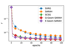
(a) mushrooms

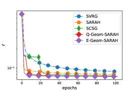
(b) w8a

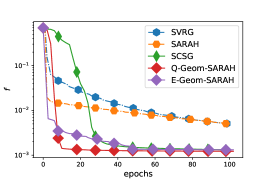
(c) ijcnn1

Figure 1: Comparison of convergence with respect to functional value for different high precision VR methods.

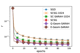
(a) mushrooms

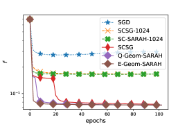
(b) w8a

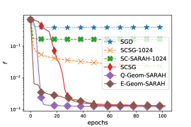
(c) ijcnn1

Figure 2: Comparison of convergence with respect to functional value for different low precision VR methods.

4.3 Better rates for non-adaptive Geom-SARAH

In this section, we provide the versions of our algorithms, which are neither almost universal nor $\epsilon$-independent, but they either reach the known lower bounds or best achievable results known in literature. We include this result for two reasons. Firstly, we want to show there is a small gap between results in Section 4.2 and the best results, which might be obtained. We conjecture that this gap is inevitable. Secondly, our complexity result for the functional gap beats the best known complexity result known in literature which is $\mathcal{O}\left(\log^{3}B\left[B+\frac{\sqrt{B}}{\mu}\right]\log(\frac{1}{\epsilon})\right)$, where $B=\mathcal{O}\left(\frac{\sigma^{2}}{\mu\epsilon^{2}}\wedge n\right)$ (Zhou et al., 2018) , where our complexity result does not involve $\log^{3}B$ factor. Finally, we obtain very interesting result for the norm of the gradient, which we discuss later in this section. The proofs are relegated into Appendix A.

Theorem 5 (Non-adaptive).

Set the hyperparameters as

$$\eta_{j}=\frac{b_{j}}{2L\sqrt{m_{j}}},\quad b_{j}\leq\sqrt{m_{j}},\quad B_{j}=m_{j}=B.$$

1. If $B=\left(\frac{\sigma^{2}}{4\mu\epsilon^{2}}\wedge n\right)$ and $\delta=0$ then

   $$\mathbb{E}\mathrm{Comp}_{f}(\epsilon)=\mathcal{O}\left(\left(B+\frac{\sqrt{B}L}{\mu}\right)\log\left(\frac{\Delta_{f}}{\epsilon^{2}}\right)\right)$$

2. If $B=\left(\left\{\frac{8\sigma^{2}}{\epsilon^{2}}+\frac{8\sigma^{4/3}L^{2/3}}{\epsilon^{4/3}\mu^{2/3}}\right\}\wedge n\right)$ and $\delta=0$ then

   $$\mathbb{E}\mathrm{Comp}_{g}(\epsilon)=\mathcal{O}\left(\left(B+\frac{\sqrt{B}L}{\mu}\right)\log\frac{L\Delta_{f}}{\sqrt{B}\epsilon^{2}}\right),$$

Looking into these result, there is one important thing to note. While these methods reach state-of-the-art performance for PL objectives, they provide no guarantees for the case $\mu=0$.

For the ease of presentation we assume $\sigma^{2},\Delta_{f},L={\cal O}(1)$. For Q-Geom-SARAH, we can see that in term of $\tilde{{\cal O}}$ notation, we match the best reachable rate in case $\mu=0$. For the case $\mu>0$, we see slight degradation in performance for both high and low precision regimes. For E-Geom-SARAH, we can see a bit different results. There is a $\nicefrac{{1}}{{\epsilon}}$ degradation comparing to the low precision case and exact match for high precision case with $\mu=0$. For the case $\mu>0$, E-Geom-SARAH matches the best achievable rate for high precision and also for in low precision regime in the case when rate is dominated by factor $\nicefrac{{1}}{{\epsilon^{2}}}$. Comparison to other methods together with the dependence on parameters can be found in Tables 1 and 2.

One interesting fact to note is that in the second case of Theorem 5, if $\mu\sim\epsilon$ and $L,\Delta_{f},\sigma^{2}=\mathcal{O}(1)$, $B\sim 1/\epsilon^{2}$ and

$$\mathbb{E}\mathrm{Comp}_{g}(\epsilon)=\mathcal{O}\left(\frac{1}{\epsilon^{2}}\log\left(\frac{1}{\epsilon}\right)\right).$$

This is even logarithmically better than the rate $\mathcal{O}(\epsilon^{-2}\log^{3}(1/\mu))$ obtained by Allen-Zhu (2018) for strongly-convex functions. Note that a strongly convex function with modulus $\mu$ is always $\mu$-PL. We plan to further investigate this strong result in the future.

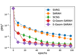
(a) mushrooms

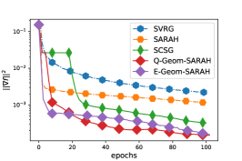
(b) w8a

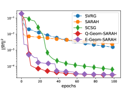
(c) ijcnn1

Figure 3: Comparison of convergence with respect to norm of the gradient for different high precision VR methods.

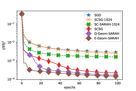
(a) mushrooms

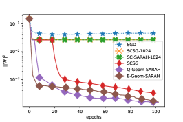
(b) w8a

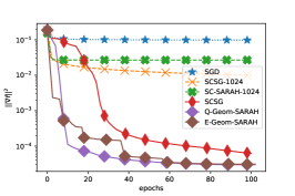
(c) ijcnn1

Figure 4: Comparison of convergence with respect to norm of the gradient for different low precision VR methods.

5 Experiments

To support our theoretical result, we conclude several experiments using logistic regression with non-convex penalty. The objective that we minimize is of the form

$$-\frac{1}{n}\sum_{i=1}^{n}\left[f_{i}(x)\overset{\triangle}{=}\log\left(1+e^{-y_{i}w_{i}^{\top}x}\right)+\frac{\lambda}{2}\sum_{j=1}^{d}\frac{x_{j}^{2}}{1+x_{j}^{2}}\right],$$

where $w_{i}$’s are the features, $y_{i}$’s the labels and $\lambda>0$ is a regularization parameter. This fits to our framework with $L_{f_{i}}=\nicefrac{{\left\lVert a_{i}\right\rVert^{2}}}{{4}}+\lambda$. We compare our adaptive methods against state-of-the-art methods in this framework–SARAH Nguyen et al. (2019), SVRG Reddi et al. (2016), Spiderboost Wang et al. (2018), adaptive and fixed version of SCSG Lei et al. (2017) with big batch sizes $B=cj^{3/2}\wedge n$ for some constant $c$. We use all the methods with their theoretical parameters. We use SARAH and Spiderboost with constant step size $\nicefrac{{1}}{{2L}}$, which implies batch size to be $b=\sqrt{n}$. In this scenario, Spiderboost and SARAH are the same algorithm and we refer to both as SARAH. The same step size is also used for SVRG which requires batch size $b=n^{2/3}$. The same applies to SCSG and our methods and we adjust parameter accordingly, e.g. this applies that for our methods we set $b_{j}=\sqrt{m_{j}}$. For E-Geom-SARAH, we chose $\alpha=2$. We also include SGD methods with the same step size for comparison. All the experiments are run with $\lambda=0.1$. We use three dataset from LibSVM: mushrooms ($n=8,124,p=112$), w8a ($n=49,749,p=300$), and ijcnn1 ($n=49,990,p=22$).

We run two sets of experiments– low and high precision. Firstly, we compare our adaptive methods with the ones that can guarantee convergence to arbitrary precision $\epsilon$ – SARAH, SVRG and adaptive SCSG. Secondly, we conclude the experiment where we compare our adaptive methods against ones that should provide better convergence in low precision regimes– SARAH and SVRG with big batch size $B=1024$, adaptive SCSG and SGD with batch size equal to $32$. For all the experiments, we display functional value and norm of the gradient with respect to number of epochs (IFO calls divided by $n$). For all Figures 1, 2, 3 and 4, we can see that our adaptive method perfoms the best in all the regimes and the only method that reaches comparable performance is SCSG.

6 Conclusion

We have presented two new methods Q-Geom-SARAH and E-Geom-SARAH, a gradient-based algorithm for the non-convex finite-sum/online optimization problem. We have shown that our methods are both $\epsilon$-independent and almost-universal algorithms. We obtain these properties via geometrization and careful batch size construction. Our methods provide strictly better results comparing to other methods as these are the only methods which can adapt to multiple regimes, i.e. low/high precision or PL with $\mu=0/\mu>0$. Moreover, we show that the obtained complexity is closed to or even matches the best achievable one in all the regimes.

Appendix

Appendix A Proofs

A.1 Proof of Lemma 1

By definition,

$$E(D_{N}-D_{N+1}) =\sum_{n\geq 0}(D_{k}-D_{k+1})\cdot\gamma^{k}(1-\gamma)$$

$$=(1-\gamma)(D_{0}-\sum_{k\geq 1}D_{k}(\gamma^{k-1}-\gamma^{k}))=(1-\gamma)\left(\frac{1}{\gamma}D_{0}-\sum_{k\geq 0}D_{k}(\gamma^{k-1}-\gamma^{k})\right)$$

$$=(1-\gamma)\left(\frac{1}{\gamma}D_{0}-\frac{1}{\gamma}\sum_{k\geq 0}D_{k}\gamma^{k}(1-\gamma)\right)=\frac{1-\gamma}{\gamma}(D_{0}-\mathbb{E}{D_{N}}),$$

where the last equality is implied by the condition that $\mathbb{E}{|D_{N}|}<\infty$.

In order to use Lemma 1, one needs to show $\mathbb{E}{|D_{N}|}<\infty$. We start with the following lemma as the basis to apply geometrization. The proof is distracting and relegated to the end of this section.

Lemma 6.

Assume that $\eta_{j}L\leq 1$. Then $\mathbb{E}|D_{N_{j}}^{(s)}|<\infty$ for $s=1,2,3$, where

$$D_{k}^{(1)}=\mathbb{E}_{j}\left\lVert\nu^{(j)}_{k}-\nabla f(x^{(j)}_{k})\right\rVert^{2},\quad D_{k}^{(2)}=\mathbb{E}_{j}f(x^{(j)}_{k}),\quad D_{k}^{(3)}=\mathbb{E}_{j}\left\lVert\nabla f(x^{(j)}_{k})\right\rVert^{2},$$

and $\mathbb{E}_{j}$ denotes the expectation over the randomness in $j$-th outer loop.

Based on Lemma 6, we prove two lemmas, which helps us to establish the sequence that is used to prove convergence. Throughout the rest of the section we assume that assumption 1 and 2 hold.

Lemma 7.

For any $j$,

$$\mathbb{E}_{j}\left\lVert\nu^{(j)}_{N_{j}}-\nabla f(\tilde{x}_{j})\right\rVert^{2}\leq\frac{m_{j}\eta_{j}^{2}L^{2}}{b_{j}^{2}}\mathbb{E}_{j}\left\lVert\nu^{(j)}_{N_{j}}\right\rVert^{2}+\frac{\sigma^{2}I(B_{j}\leq n)}{B_{j}},$$

where $\mathbb{E}_{j}$ denotes the expectation over the randomness in $j$-th outer loop.

Proof.

Let $\mathbb{E}_{j,k}$ and $\operatorname{Var}_{j,k}$ denote the expectation and variance operator over the randomness of $\mathcal{I}^{(j)}_{k}$. Since $\mathcal{I}^{(j)}_{k}$ is independent of $x^{(j)}_{k}$,

$$\mathbb{E}_{j,k}\nu^{(j)}_{k+1}=\nu^{(j)}_{k}+(\nabla f(x^{(j)}_{k+1})-\nabla f(x^{(j)}_{k})).$$

Thus,

$$\nu^{(j)}_{k+1}-\nabla f(x^{(j)}_{k+1})=\nu^{(j)}_{k}-\nabla f(x^{(j)}_{k})+\left(\nu^{(j)}_{k+1}-\nu^{(j)}_{k}-\mathbb{E}_{j,k}(\nu^{(j)}_{k+1}-\nu^{(j)}_{k})\right).$$

Since $\mathcal{I}^{(j)}_{k}$ is independent of $(\nu^{(j)}_{k},x^{(j)}_{k})$,

$$\operatorname{Cov}_{j,k}\left(\nu^{(j)}_{k}-\nabla f(x^{(j)}_{k}),\nu^{(j)}_{k+1}-\nu^{(j)}_{k}\right)=0.$$

As a result,

$$\mathbb{E}_{j,k}\left\lVert\nu^{(j)}_{k+1}-\nabla f(x^{(j)}_{k+1})\right\rVert^{2}=\left\lVert\nu^{(j)}_{k}-\nabla f(x^{(j)}_{k})\right\rVert^{2}+\operatorname{Var}_{j,k}(\nu^{(j)}_{k+1}-\nu^{(j)}_{k}).$$ (13)

By Lemma 14,

$$\operatorname{Var}_{j,k}(\nu^{(j)}_{k+1}-\nu^{(j)}_{k})=\operatorname{Var}\left(\frac{1}{b_{j}}\sum_{i\in\mathcal{I}^{(j)}_{k}}(\nabla f_{i}(x^{(j)}_{k+1})-\nabla f_{i}(x^{(j)}_{k}))\right)$$

$$\leq\frac{1}{b_{j}}\frac{1}{n}\sum_{i=1}^{n}\left\lVert\nabla f_{i}(x^{(j)}_{k+1})-\nabla f_{i}(x^{(j)}_{k})-(\nabla f(x^{(j)}_{k+1})-\nabla f(x^{(j)}_{k}))\right\rVert^{2}$$ (14)

$$\leq\frac{1}{b_{j}}\frac{1}{n}\sum_{i=1}^{n}\left\lVert\nabla f_{i}(x^{(j)}_{k+1})-\nabla f_{i}(x^{(j)}_{k})\right\rVert^{2}.$$

Finally by assumption 1,

$$\frac{1}{n}\sum_{i=1}^{n}\left\lVert\nabla f_{i}(x^{(j)}_{k+1})-\nabla f_{i}(x^{(j)}_{k})\right\rVert^{2}\leq L^{2}\left\lVert x^{(j)}_{k+1}-x^{(j)}_{k}\right\rVert^{2}=\eta_{j}^{2}L^{2}\left\lVert\nu^{(j)}_{k}\right\rVert^{2}.$$

By (13),

$$\mathbb{E}_{j,k}\left\lVert\nu^{(j)}_{k+1}-\nabla f(x^{(j)}_{k+1})\right\rVert^{2}=\left\lVert\nu^{(j)}_{k}-\nabla f(x^{(j)}_{k})\right\rVert^{2}+\frac{\eta_{j}^{2}L^{2}}{b_{j}}\left\lVert\nu^{(j)}_{k}\right\rVert^{2}.$$

Let $k=N_{j}$ and take expectation over all randomness in $\mathbb{E}_{j}$. By Lemma 6, we can apply Lemma 1 on $D_{k}=\mathbb{E}_{j}\left\lVert\nu^{(j)}_{k}-\nabla f(x^{(j)}_{k})\right\rVert^{2}$. Then we have

$$0 \leq\mathbb{E}_{j}\left(\|\nu^{(j)}_{N_{j}}-\nabla f(x^{(j)}_{N_{j}})\|^{2}-\|\nu^{(j)}_{N_{j}+1}-\nabla f(x^{(j)}_{N_{j}+1})\|^{2}\right)+\frac{\eta_{j}^{2}L^{2}}{b_{j}}\mathbb{E}_{j}\|\nu^{(j)}_{N_{j}}\|^{2}$$

$$=\frac{b_{j}}{m_{j}}\mathbb{E}_{j}\left(\|\nu^{(j)}_{0}-\nabla f(x^{(j)}_{0})\|^{2}-\|\nu^{(j)}_{N_{j}}-\nabla f(x^{(j)}_{N_{j}})\|^{2}\right)+\frac{\eta_{j}^{2}L^{2}}{b_{j}}\mathbb{E}_{j}\|\nu^{(j)}_{N_{j}}\|^{2}.$$

Finally, by Lemma 14,

$$\mathbb{E}_{j}\|\nu^{(j)}_{0}-\nabla f(x^{(j)}_{0})\|^{2}\leq\frac{\sigma^{2}I(B_{j}<n)}{B_{j}}.$$ (15)

The proof is then completed. ∎

Lemma 8.

For any $j$,

$$\mathbb{E}_{j}\left\lVert\nabla f(\tilde{x}_{j})\right\rVert^{2}\leq\frac{2b_{j}}{\eta_{j}m_{j}}\mathbb{E}_{j}(f(\tilde{x}_{j-1})-f(\tilde{x}_{j}))+\mathbb{E}_{j}\left\lVert\nu^{(j)}_{N_{j}}-\nabla f(\tilde{x}_{j})\right\rVert^{2}-(1-\eta_{j}L)\mathbb{E}_{j}\left\lVert\nu^{(j)}_{N_{j}}\right\rVert^{2},$$

where $\mathbb{E}_{j}$ denotes the expectation over the randomness in $j$-th outer loop.

Proof.

By assumption (1),

$$f(x^{(j)}_{k+1}) \leq f(x^{(j)}_{k})+\left\langle\nabla f(x^{(j)}_{k}),x^{(j)}_{k+1}-x^{(j)}_{k}\right\rangle+\frac{L}{2}\left\lVert x^{(j)}_{k}-x^{(j)}_{k+1}\right\rVert^{2}$$

$$=f(x^{(j)}_{k})-\eta\left\langle\nabla f(x^{(j)}_{k}),\nu^{(j)}_{k}\right\rangle+\frac{\eta_{j}^{2}L}{2}\left\lVert\nu^{(j)}_{k}\right\rVert^{2}$$

$$=f(x^{(j)}_{k})+\frac{\eta_{j}}{2}\left\lVert\nu^{(j)}_{k}-\nabla f(x^{(j)}_{k})\right\rVert^{2}-\frac{\eta_{j}}{2}\left\lVert\nabla f(x^{(j)}_{k})\right\rVert^{2}-\frac{\eta_{j}}{2}\left\lVert\nu^{(j)}_{k}\right\rVert^{2}+\frac{\eta_{j}^{2}L}{2}\left\lVert\nu^{(j)}_{k}\right\rVert^{2}.$$ (16)

Let $j=N_{j}$ and take expectation over all randomness in $\mathbb{E}_{j}$. By Lemma 6, we can apply Lemma 1 with $D_{k}=\mathbb{E}_{j}f(x^{(j)}_{k})$ and $D_{k}=\mathbb{E}_{j}\left\lVert\nabla f(x^{(j)}_{k})\right\rVert^{2}$. Thus,

$$0 \leq\mathbb{E}_{j}\left(f(x^{(j)}_{N_{j}})-f(x^{(j)}_{N_{j}+1})\right)+\frac{\eta_{j}}{2}\mathbb{E}_{j}\left\lVert\nu^{(j)}_{N_{j}}-\nabla f(x^{(j)}_{N_{j}})\right\rVert^{2}-\frac{\eta_{j}}{2}\mathbb{E}_{j}\left\lVert\nabla f(x^{(j)}_{N_{j}})\right\rVert^{2}-\frac{\eta_{j}}{2}(1-\eta_{j}L)\mathbb{E}_{j}\left\lVert\nu^{(j)}_{N_{j}}\right\rVert^{2}$$

$$=\frac{b_{j}}{m_{j}}\mathbb{E}_{j}\left(f(x^{(j)}_{0})-f(x^{(j)}_{N_{j}})\right)+\frac{\eta_{j}}{2}\mathbb{E}_{j}\left\lVert\nu^{(j)}_{N_{j}}-\nabla f(x^{(j)}_{N_{j}})\right\rVert^{2}-\frac{\eta_{j}}{2}\mathbb{E}_{j}\left\lVert\nabla f(x^{(j)}_{N_{j}})\right\rVert^{2}-\frac{\eta_{j}}{2}(1-\eta_{j}L)\mathbb{E}_{j}\left\lVert\nu^{(j)}_{N_{j}}\right\rVert^{2}$$

$$=\frac{b_{j}}{m_{j}}\mathbb{E}_{j}\left(f(\tilde{x}_{j-1})-f(\tilde{x}_{j})\right)+\frac{\eta_{j}}{2}\mathbb{E}_{j}\left\lVert\nu^{(j)}_{N_{j}}-\nabla f(x^{(j)}_{N_{j}})\right\rVert^{2}-\frac{\eta_{j}}{2}\mathbb{E}_{j}\left\lVert\nabla f(\tilde{x}_{j})\right\rVert^{2}-\frac{\eta_{j}}{2}(1-\eta_{j}L)\mathbb{E}_{j}\left\lVert\nu^{(j)}_{N_{j}}\right\rVert^{2}.$$

The proof is then completed. ∎

Theorem 2 is then proved by combining Lemma 7 and Lemma 8.

Proof of Theorem 2.

By Lemma 7 and Lemma 8,

$$\mathbb{E}\|\nabla f(\tilde{x}_{j})\|^{2} \leq\frac{2b_{j}}{\eta_{j}m_{j}}\mathbb{E}(f(\tilde{x}_{j-1})-f(\tilde{x}_{j}))+\frac{\sigma^{2}I(B_{j}<n)}{B_{j}}-\left(1-\eta_{j}L-\frac{m_{j}\eta_{j}^{2}L^{2}}{b_{j}^{2}}\right)\mathbb{E}\|\nu^{(j)}_{N_{j}}\|^{2}.$$

Under condition (9),

$$1-\eta_{j}L-\frac{m_{j}(\eta_{j}L)^{2}}{b_{j}^{2}}\geq 1-\frac{1}{2}-\frac{1}{4}\geq 0,$$

which concludes the proof. ∎

Proof of Lemma 6.

By (14) and assumption 2,

$$\operatorname{Var}_{j,k}(\nu^{(j)}_{k+1}-\nu^{(j)}_{k}) \leq\frac{2}{b_{j}n}\left(\sum_{i=1}^{n}\left\lVert\nabla f_{i}(x^{(j)}_{k+1})-\nabla f(x^{(j)}_{k+1})\right\rVert^{2}+\sum_{i=1}^{n}\left\lVert\nabla f_{i}(x^{(j)}_{k})-\nabla f(x^{(j)}_{k})\right\rVert^{2}\right)$$

$$\leq\frac{4\sigma^{2}}{b_{j}}\leq 4\sigma^{2}.$$

By (13) and taking expectation over all randomness in epoch $j$,

$$\mathbb{E}_{j}\left\lVert\nu^{(j)}_{k+1}-\nabla f(x^{(j)}_{k+1})\right\rVert^{2}\leq\mathbb{E}_{j}\left\lVert\nu^{(j)}_{k}-\nabla f(x^{(j)}_{k})\right\rVert^{2}+4\sigma^{2}.$$

Then

$$\mathbb{E}_{j}\left\lVert\nu^{(j)}_{k}-\nabla f(x^{(j)}_{k})\right\rVert^{2}\leq\left\lVert\nu^{(j)}_{0}-\nabla f(x^{(j)}_{0})\right\rVert^{2}+4k\sigma^{2}\leq(4k+1)\sigma^{2}=\mathrm{poly}(k),$$ (17)

where the last inequality uses (15). By remark 1, we obtain that $\mathbb{E}|D_{N_{j}}^{(1)}|<\infty$.

On the other hand, by (16), since $\eta_{j}L\leq 1$,

$$f(x^{(j)}_{k+1})+\frac{\eta_{j}}{2}\left\lVert\nabla f(x^{(j)}_{k})\right\rVert^{2}\leq f(x^{(j)}_{k})+\frac{\eta_{j}}{2}\left\lVert\nu^{(j)}_{k}-\nabla f(x^{(j)}_{k})\right\rVert^{2}\leq f(x^{(j)}_{k})+(2k+1)\eta_{j}\sigma^{2},$$

where the last inequality uses (17). Let

$$M^{(j)}_{k}=f(x^{(j)}_{k+1})-f(x^{\star})+\frac{\eta_{j}}{2}\left\lVert\nabla f(x^{(j)}_{k})\right\rVert^{2}.$$

Then

$$M^{(j)}_{k}\leq M^{(j)}_{k-1}+(2k+1)\eta_{j}\sigma^{2}.$$

Applying the above inequality recursively, we have

$$M^{(j)}_{k}\leq M^{(j)}_{0}+(k^{2}+2k)\eta_{j}\sigma^{2}=\mathrm{poly}(k).$$

As a result,

$$0\leq f(x^{(j)}_{k+1})-f(x^{\star})\leq M^{(j)}_{k-1}=\mathrm{poly}(k),\quad 0\leq\left\lVert\nabla f(x^{(j)}_{k})\right\rVert^{2}\leq\frac{1}{\eta_{j}}M^{(j)}_{k}=\mathrm{poly}(k).$$

By remark 1, we obtain that

$$\mathbb{E}|f(x^{(j)}_{N_{j}})-f(x^{\star})|<\infty,\quad\mathbb{E}|D_{N_{j}}^{(3)}|=\mathbb{E}\left\lVert\nabla f(x^{(j)}_{N_{j}})\right\rVert^{2}<\infty.$$

Since $f(x^{\star})>-\infty$, $\mathbb{E}|D_{N_{j}}^{(2)}|<\infty$. ∎

A.2 Preparation for Complexity Analysis

Although Theorem 3 and 4 consider the tail-randomized iterate, we start by studying two conventional output – the randomized iterate and the last iterate. Throughout this subsection we let

$$\lambda_{j}=\eta_{j}m_{j}/b_{j}.$$

The first lemma states a bound for expected gradient norm of the randomized iterate.

Lemma 9.

Given any positive integer $T$, let $\mathcal{R}$ be a random variable supported on $\{1,\ldots,T\}$ with

$$\mathbb{P}(\mathcal{R}=j)\propto\lambda_{j}$$

Then

$$\mathbb{E}\left\lVert\nabla f(x_{\mathcal{R}})\right\rVert^{2}\leq\frac{2\mathbb{E}\left(f(\tilde{x}_{0})-f(x^{\star})\right)+\sigma^{2}\sum_{j=1}^{T}\lambda_{j}I(B_{j}<n)/B_{j}}{\sum_{j=1}^{T}\lambda_{j}}$$

Proof.

By Theorem 2,

$$\lambda_{j}\mathbb{E}\left\lVert\nabla f(\tilde{x}_{j})\right\rVert^{2}\leq 2\left(\mathbb{E}f(\tilde{x}_{j-1})-\mathbb{E}f(\tilde{x}_{j})\right)+\frac{\sigma^{2}\lambda_{j}I(B_{j}<n)}{B_{j}}.$$

By definition,

$$\mathbb{E}\left\lVert\nabla f(x_{\mathcal{R}})\right\rVert^{2}=\frac{\sum_{j=1}^{T}\mathbb{E}\left\lVert\nabla f(\tilde{x}_{j})\right\rVert^{2}\lambda_{j}}{\sum_{j=1}^{T}\lambda_{j}}$$

$$\leq\frac{2\sum_{j=1}^{T}\left(\mathbb{E}f(\tilde{x}_{j-1})-\mathbb{E}f(\tilde{x}_{j})\right)+\sigma^{2}\sum_{j=1}^{T}\lambda_{j}I(B_{j}<n)/B_{j}}{\sum_{j=1}^{T}\lambda_{j}}$$

$$=\frac{2\left(\mathbb{E}f(\tilde{x}_{0})-\mathbb{E}f(\tilde{x}_{T})\right)+\sigma^{2}\sum_{j=1}^{T}\lambda_{j}I(B_{j}<n)/B_{j}}{\sum_{j=1}^{T}\lambda_{j}}.$$

The proof is then completed by the fact that $f(\tilde{x}_{T})\geq f(x^{\star})$. ∎

The next lemma provides contraction results for expected gradient norm and function value suboptimality of the last iterate.

Lemma 10.

Define the following Lyapunov function

$$\mathcal{L}_{j}=\mathbb{E}\left(\lambda_{j}\left\lVert\nabla f(\tilde{x}_{j})\right\rVert^{2}+2(f(\tilde{x}_{j})-f(x^{\star}))\right).$$

Then under the assumption 3 with $\mu$ possibly being zero,

$$\mathcal{L}_{j}\leq\frac{1}{\mu\lambda_{j-1}+1}\mathcal{L}_{j-1}+\frac{\sigma^{2}\lambda_{j}I(B_{j}<n)}{B_{j}},$$ (18)

and

$$\mathbb{E}\left(f(\tilde{x}_{j})-f(x^{\star})\right)\leq\frac{1}{\mu\lambda_{j}+1}\mathbb{E}\left(f(\tilde{x}_{j-1})-f(x^{\star})\right)+\frac{\lambda_{j}}{\mu\lambda_{j}+1}\frac{\sigma^{2}I(B_{j}<n)}{2B_{j}}.$$ (19)

Proof.

When $\mu=0$, the lemma is a direct consequence of Theorem 2. Assume $\mu>0$ throughout the rest of the proof. Let

$$\chi_{j}=\frac{\mu\lambda_{j}}{\mu\lambda_{j}+1}.$$

Then by assumption 3,

$$\mathbb{E}(f(\tilde{x}_{j})-f(x^{\star})) =(1-\chi_{j})\mathbb{E}(f(\tilde{x}_{j})-f(x^{\star}))+\chi_{j}\mathbb{E}(f(\tilde{x}_{j})-f(x^{\star}))$$

$$\leq(1-\chi_{j})\mathbb{E}(f(\tilde{x}_{j})-f(x^{\star}))+\frac{\chi_{j}}{2\mu}\mathbb{E}\left\lVert\nabla f(\tilde{x}_{j})\right\rVert^{2}$$

$$=\frac{1}{2(\mu\lambda_{j}+1)}\left(\lambda_{j}\mathbb{E}\left\lVert\nabla f(\tilde{x}_{j})\right\rVert^{2}+2\mathbb{E}(f(\tilde{x}_{j})-f(x^{\star}))\right)$$

$$=\frac{1}{2(\mu\lambda_{j}+1)}\mathcal{L}_{j}.$$

By Theorem 2,

$$\mathcal{L}_{j} \leq 2\mathbb{E}(f(\tilde{x}_{j-1})-f(x^{\star}))+\frac{\sigma^{2}\lambda_{j}I(B_{j}<n)}{B_{j}}$$

$$\leq\frac{1}{\mu\lambda_{j-1}+1}\mathcal{L}_{j-1}+\frac{\sigma^{2}\lambda_{j}I(B_{j}<n)}{B_{j}}.$$

On the other hand, by Theorem 5,

$$2\mu\mathbb{E}(f(\tilde{x}_{j})-f(x^{\star}))\leq\mathbb{E}\|\nabla f(\tilde{x}_{j})\|^{2}\leq\frac{2}{\lambda_{j}}\mathbb{E}(f(\tilde{x}_{j-1})-f(\tilde{x}_{j}))+\frac{\sigma^{2}I(B_{j}<n)}{B_{j}}.$$

Rearranging terms concludes the proof. ∎

The third lemma shows that $\mathcal{L}_{j}$ and $\mathbb{E}(f(\tilde{x}_{j})-f(x^{\star}))$ are uniformly bounded.

Lemma 11.

For any $j>0$,

$$\mathcal{L}_{j}\leq\Delta_{L}\overset{\triangle}{=}2\Delta_{f}+\left(\sum_{t:B_{t}<n}\frac{\lambda_{t}}{B_{t}}\right)\sigma^{2}.$$

Proof.

By (18), since $\mu\geq 0$,

$$\mathcal{L}_{j}\leq\mathcal{L}_{j-1}+\frac{\sigma^{2}\lambda_{j}I(B_{j}<n)}{B_{j}}.$$

Moreover, by Theorem 2,

$$\mathcal{L}_{1}\leq 2\mathbb{E}(f(\tilde{x}_{0})-f(x^{\star}))+\frac{\lambda_{1}\sigma^{2}I(B_{1}<n)}{B_{1}}.$$

Telescoping the above inequalities yields the bound for $\mathcal{L}_{j}$. ∎

The last lemma states refined bounds for $\mathbb{E}\left\lVert\nabla f(\tilde{x}_{j})\right\rVert^{2}$ and $\mathbb{E}(f(\tilde{x}_{j})-f(x^{\star}))$ based on Lemma 10 and Lemma 11.

Lemma 12.

Fix any constant $c\in(0,1)$. Suppose $B_{j}$ can be written as

$$B_{j}=\lceil\tilde{B}_{j}\wedge n\rceil,$$

for some strictly increasing sequence $\tilde{B}_{j}$. Assume that $\lambda_{j}$ is non-decreasing and

$$\frac{\tilde{B}_{j-1}\lambda_{j}}{\tilde{B}_{j}\lambda_{j-1}}\geq\sqrt{c}.$$

Let

$$T_{\mu}(c)=\min\{j:\lambda_{j}>1/\mu c\},\quad T_{n}=\min\{j:\tilde{B}_{j}\geq n\},$$

where $T_{\mu}(c)=\infty$ if no such $j$ exists, e.g. for $\mu=0$. Then for any $j>T_{\mu}(c)$,

$$\mathbb{E}\left\lVert\nabla f(\tilde{x}_{j})\right\rVert^{2}\leq\min\left\{\left(\prod_{t=T_{\mu}(c)}^{j-1}\frac{1}{\mu\lambda_{t}}\right)\frac{\Delta_{L}}{\lambda_{j}}+\frac{\sigma^{2}I(j>T_{\mu}(c))}{(1-\sqrt{c})\tilde{B}_{j}},\left(\frac{1}{\mu\lambda_{T_{n}}+1}\right)^{(j-T_{n})_{+}}\frac{\Delta_{L}}{\lambda_{j}}\right\},$$

and

$$\mathbb{E}\left(f(\tilde{x}_{j})-f(x^{\star})\right)\leq\min\left\{\left(\prod_{t=T_{\mu}(c)+1}^{j}\frac{1}{\mu\lambda_{t}}\right)\Delta_{L}+\frac{\sigma^{2}I(j>T_{\mu}(c))}{2(1-\sqrt{c})\mu\tilde{B}_{j}},\left(\frac{1}{\mu\lambda_{T_{n}}+1}\right)^{(j-T_{n})_{+}}\Delta_{L}\right\},$$

where $\prod_{t=a}^{b}c_{t}=1$ if $a>b$.

Proof.

We first prove the bounds involving $T_{\mu}(c)$. Assume $T_{\mu}(c)<\infty$. Then for $j>T_{\mu}(c)$,

$$\frac{1}{\mu\lambda_{j}+1}\leq\frac{1}{\mu\lambda_{j-1}+1}<\frac{1}{\mu\lambda_{j-1}}<c.$$ (20)

By (18), (19) and the condition that $\lambda_{j}\geq\lambda_{j-1}$, we have

$$\mathcal{L}_{j}\leq\frac{1}{\mu\lambda_{j-1}}\mathcal{L}_{j-1}+\frac{\sigma^{2}\lambda_{j}I(B_{j}<n)}{B_{j}}\leq\frac{1}{\mu\lambda_{j-1}}\mathcal{L}_{j-1}+\frac{\sigma^{2}\lambda_{j}}{\tilde{B}_{j}},$$

and

$$\mathbb{E}\left(f(\tilde{x}_{j})-f(x^{\star})\right) \leq\frac{1}{\mu\lambda_{j}}\mathbb{E}\left(f(\tilde{x}_{j-1})-f(x^{\star})\right)+\frac{\sigma^{2}I(B_{j}<n)}{2\mu B_{j}}$$

$$\leq\frac{1}{\mu\lambda_{j}}\mathbb{E}\left(f(\tilde{x}_{j-1})-f(x^{\star})\right)+\frac{\sigma^{2}}{2\mu\tilde{B}_{j}}.$$

Applying the above inequalities recursively and using Lemma 11 and (20), we obtain that

$$\lambda_{j}\mathbb{E}\left\lVert\nabla f(\tilde{x}_{j})\right\rVert^{2} \leq\mathcal{L}_{j}\leq\left(\prod_{t=T_{\mu}(c)}^{j-1}\frac{1}{\mu\lambda_{t}}\right)\mathcal{L}_{T_{\mu}(c)}+\sigma^{2}\sum_{t=T_{\mu}(c)+1}^{j}\frac{c^{j-t}\lambda_{t}}{\tilde{B}_{t}}$$

$$\stackrel{{\scriptstyle(i)}}{{\leq}}\left(\prod_{t=T_{\mu}(c)}^{j-1}\frac{1}{\mu\lambda_{t}}\right)\Delta_{L}+\sigma^{2}\sum_{t=T_{\mu}(c)+1}^{j}\frac{(\sqrt{c})^{j-t}\lambda_{j}}{\tilde{B}_{j}}$$

$$=\left(\prod_{t=T_{\mu}(c)}^{j-1}\frac{1}{\mu\lambda_{t}}\right)\Delta_{L}+\frac{\sigma^{2}\lambda_{j}}{(1-\sqrt{c})\tilde{B}_{j}}$$

where (i) uses the condition that $\tilde{B}_{j-1}\lambda_{j}/\tilde{B}_{j}\lambda_{j-1}\geq\sqrt{c}$ and thus $B_{t}\geq B_{j}(\sqrt{c})^{(j-t)}$. Similarly,

$$\mathbb{E}\left(f(\tilde{x}_{j})-f(x^{\star})\right)\leq\left(\prod_{t=T_{\mu}(c)+1}^{j}\frac{1}{\mu\lambda_{t}}\right)\Delta_{L}+\frac{\sigma^{2}}{2(1-\sqrt{c})\mu\tilde{B}_{j}}.$$

Next, we prove the bounds involving $T_{n}$. Similar to the previous step, the case with $j\leq T_{n}$ can be easily proved. When $j>T_{n}$, $B_{j}=n$ and thus

$$\mathcal{L}_{j}\leq\left(\frac{1}{\mu\lambda_{T_{n}}+1}\right)\mathcal{L}_{j-1},\quad\mathbb{E}\left(f(\tilde{x}_{j})-f(x^{\star})\right)\leq\left(\frac{1}{\mu\lambda_{T_{n}}+1}\right)\mathbb{E}\left(f(\tilde{x}_{j-1})-f(x^{\star})\right).$$

This implies the bounds involving $T_{n}$. ∎

Combining Lemma 9 and Lemma 12, we obtain the convergence rate of the randomized iterate.

Theorem 13.

Given any positive integer $T$, let $\mathcal{R}$ be a random variable supported on $\{T,\ldots,\lceil(1+\delta)T\rceil\}$ with

$$\mathbb{P}(\mathcal{R}=j)\propto\lambda_{j}.$$

Then under the settings of Lemma 12,

$$\mathbb{E}\left\lVert\nabla f(\tilde{x}_{\mathcal{R}})\right\rVert^{2}\leq\min\bigg{\{} \left(\prod_{t=T_{\mu}(c)}^{T-1}\frac{1}{\mu\lambda_{t}}\right)\frac{\Delta_{L}}{\lambda_{T}}+\frac{\sigma^{2}I(T>T_{\mu}(c))}{(1-\sqrt{c})\tilde{B}_{T}},\left(\frac{1}{\mu\lambda_{T_{n}}+1}\right)^{(T-T_{n})_{+}}\frac{\Delta_{L}}{\lambda_{T}},$$

$$\quad\frac{2\Delta_{L}+\sigma^{2}\sum_{j=T}^{\lceil(1+\delta)T\rceil}\lambda_{j}I(B_{j}<n)/B_{j}}{\sum_{j=T}^{\lceil(1+\delta)T\rceil}\lambda_{j}}\bigg{\}},$$

and

$$\mathbb{E}\left(f(\tilde{x}_{\mathcal{R}})-f(x^{\star})\right)\leq\min\left\{\left(\prod_{t=T_{\mu}(c)+1}^{T}\frac{1}{\mu\lambda_{t}}\right)\Delta_{L}+\frac{\sigma^{2}I(T>T_{\mu}(c))}{2(1-\sqrt{c})\mu\tilde{B}_{T}},\left(\frac{1}{\mu\lambda_{T_{n}}+1}\right)^{(T-T_{n})_{+}}\Delta_{L}\right\},$$

where $\prod_{t=a}^{b}c_{t}=1$ if $a>b$.

Proof.

By Lemma 12, for any $j\in[T,\lceil(1+\delta)T\rceil]$,

$$\mathbb{E}\left\lVert\nabla f(\tilde{x}_{j})\right\rVert^{2} \leq\min\left\{\left(\prod_{t=T_{\mu}(c)}^{j-1}\frac{1}{\mu\lambda_{t}}\right)\frac{\Delta_{L}}{\lambda_{j}}+\frac{\sigma^{2}I(j>T_{\mu}(c))}{(1-\sqrt{c})\tilde{B}_{j}},\left(\frac{1}{\mu\lambda_{T_{n}}+1}\right)^{(j-T_{n})_{+}}\frac{\Delta_{L}}{\lambda_{j}}\right\}$$

$$\leq\min\left\{\left(\prod_{t=T_{\mu}(c)}^{j-1}\frac{1}{\mu\lambda_{t}}\right)\frac{\Delta_{L}}{\lambda_{T}}+\frac{\sigma^{2}I(T>T_{\mu}(c))}{(1-\sqrt{c})\tilde{B}_{j}},\left(\frac{1}{\mu\lambda_{T_{n}}+1}\right)^{(j-T_{n})_{+}}\frac{\Delta_{L}}{\lambda_{T}}\right\}.$$

As a result,

$$\mathbb{E}\left\lVert\nabla f(\tilde{x}_{\mathcal{R}})\right\rVert^{2}=\frac{\sum_{j=T+1}^{\lceil(1+\delta)T\rceil}\lambda_{j}\mathbb{E}\left\lVert\nabla f(\tilde{x}_{j})\right\rVert^{2}}{\sum_{j=T+1}^{\lceil(1+\delta)T\rceil}\lambda_{j}}$$

$$\leq\min\left\{\left(\prod_{t=T_{\mu}(c)}^{T-1}\frac{1}{\mu\lambda_{t}}\right)\frac{\Delta_{L}}{\lambda_{T}}+\frac{\sigma^{2}I(T>T_{\mu}(c))}{(1-\sqrt{c})\tilde{B}_{j}},\left(\frac{1}{\mu\lambda_{T_{n}}+1}\right)^{(T-T_{n})_{+}}\frac{\Delta_{L}}{\lambda_{T}}\right\}.$$

Similarly we can prove the bound for $\mathbb{E}(f(\tilde{x}_{j})-f(x^{\star}))$. To prove the third bound for $\mathbb{E}\left\lVert\nabla f(\tilde{x}_{\mathcal{R}})\right\rVert^{2}$, we first notice that $\tilde{x}_{\mathcal{R}}$ can be regarded as the randomized iterate with $\tilde{x}_{T}$ being the initializer. By Lemma 9,

$$\mathbb{E}\left\lVert\nabla f(\tilde{x}_{\mathcal{R}})\right\rVert^{2}\leq\frac{2\mathbb{E}\left(f(\tilde{x}_{T})-f(x^{\star})\right)+\sigma^{2}\sum_{j=T+1}^{\lceil(1+\delta)T\rceil}\lambda_{j}I(B_{j}<n)/B_{j}}{\sum_{j=T+1}^{\lceil(1+\delta)T\rceil}\lambda_{j}}.$$

By Lemma 11,

$$\mathbb{E}\left(f(\tilde{x}_{T})-f(x^{\star})\right)\leq\Delta_{L},$$

which concludes the proof. The bound for $\mathbb{E}(f(\tilde{x}_{\mathcal{R}})-f(x^{\star}))$ can be proved similarly. ∎

A.3 Complexity Analysis: Proof of Theorem 3

Under this setting,

$$2\lambda_{j}L=\frac{2\eta_{j}m_{j}}{b_{j}}=\sqrt{m_{j}}=jI(j<\sqrt{n})+\sqrt{n}I(j\geq\sqrt{n}).$$

Let $c=1/8$. It is easy to verify that $\tilde{B}_{j-1}\lambda_{j}/\tilde{B}_{j}\lambda_{j-1}\geq 1/2>\sqrt{c}$. Moreover, by Lemma 16,

$$L\sum_{t:B_{t}<n}\frac{\lambda_{t}}{B_{t}}=\sum_{t<\sqrt{n}}\frac{1}{t}\leq 1+\log\sqrt{n}.$$

Recalling the definition of $\Delta_{L}$ in Lemma 11,

$$\Delta_{L}\leq 2\Delta_{f}+\left(\sum_{t:B_{t}<n}\frac{\lambda_{t}}{B_{t}}\right)\sigma^{2}\leq 2\left(\Delta_{f}+\frac{\sigma^{2}}{L}\log n\right)=\mathcal{O}(\Delta).$$ (21)

Now we treat each of the three terms in the bound of $\mathbb{E}\left\lVert\nabla f(\tilde{x}_{j})\right\rVert^{2}$ in Theorem 13 separately.

(First term.) Write $T_{\mu}$ for $T_{\mu}(c)=T_{\mu}(1/8)$. By definition,

$$T_{\mu}=\min\left\{j:\lambda_{j}\geq\frac{8}{\mu}\right\}=\left\{\begin{array}[]{ll}\left\lceil 16L/\mu\right\rceil&\left(\left\lceil 16L/\mu\right\rceil\leq\sqrt{n}\right)\\ \infty&(\mathrm{otherwise})\end{array}\right.$$

Let

$$T_{g1}(\epsilon)=T_{\mu}+\frac{\log(16\mu\Delta_{L}/\epsilon^{2})}{\log 8}+\frac{2\sigma}{\epsilon}.$$

When $T_{g1}(\epsilon)=\infty$, it is obvious that $T_{g}(\epsilon)\leq T_{g1}(\epsilon)$. When $T_{g1}(\epsilon)<\infty$, for any $T\geq T_{g1}(\epsilon)$,

$$\left(\prod_{t=T_{\mu}}^{T-1}\frac{1}{\mu\lambda_{t}}\right)\frac{\Delta_{L}}{\lambda_{T}}\leq c^{T-T_{\mu}}\frac{\Delta_{L}}{\lambda_{T}}\leq\left(\frac{1}{8}\right)^{\frac{\log(16\mu\Delta_{L}/\epsilon^{2})}{\log 8}}\frac{\Delta_{L}}{\lambda_{T_{\mu}}}=\frac{\epsilon^{2}}{16\mu\lambda_{T_{\mu}}}\leq\frac{\epsilon^{2}}{2}.$$

Note that $\tilde{B}_{j}=j^{2}$ in this case,

$$\frac{\sigma^{2}}{(1-\sqrt{c})\tilde{B}_{T}}\leq\frac{2\sigma^{2}}{T^{2}}\leq\frac{\epsilon^{2}}{2}.$$

Recalling the definition (7) of $T_{g}(\epsilon)$, we obtain that

$$T_{g}(\epsilon)\leq T_{g1}(\epsilon).$$

(Second term.) By definition,

$$T_{n}=\min\{j:B_{j}=n\}=\lceil\sqrt{n}\rceil,\quad\lambda_{T_{n}}=T_{n}/2L.$$

Let

$$T_{g2}(\epsilon)=T_{n}+\left(1+\frac{2L}{\mu\sqrt{n}}\right)\log\left(\frac{2L\Delta_{L}}{\sqrt{n}\epsilon^{2}}\right).$$

By Lemma 16,

$$T_{g2}(\epsilon)-T_{n}\geq\frac{\log(2L\Delta_{L}/\sqrt{n}\epsilon^{2})}{\log(1+\mu\sqrt{n}/2L)}.$$

When $T\geq T_{g2}(\epsilon)$,

$$\left(\frac{1}{\mu\lambda_{T_{n}}+1}\right)^{(T-T_{n})_{+}}\frac{\Delta_{L}}{\lambda_{T}}\leq\frac{\sqrt{n}\epsilon^{2}}{2L\Delta_{L}}\frac{\Delta_{L}}{\lambda_{T_{n}}}\leq\epsilon^{2}.$$

Therefore, we have

$$T_{g}(\epsilon)\leq T_{g2}(\epsilon).$$

(Third term.) Note that

$$2L\sum_{j=T}^{2T}\lambda_{j}I(B_{j}<n)/B_{j}=\sum_{j=T}^{2T}I(j<\sqrt{n})/j\leq\sum_{j=T}^{2T}I(j<\sqrt{n})/T\leq\frac{T+1}{T}\leq 2.$$

and

$$2L\sum_{j=T}^{2T}\lambda_{j}=\sum_{j=T}^{2T}\left(jI(j<\sqrt{n})+\sqrt{n}I(j\geq\sqrt{n})\right)\geq\sum_{j=T}^{2T}(T\wedge\sqrt{n})\geq T^{2}\wedge\sqrt{n}T.$$

Let

$$\tilde{\Delta}_{L}=2L\Delta_{L}+2\sigma^{2}.$$

By Theorem 13,

$$\mathbb{E}\left\lVert\nabla f(\tilde{x}_{j})\right\rVert^{2}\leq\frac{\tilde{\Delta}_{L}}{T^{2}\wedge\sqrt{n}T}.$$

Let

$$T_{g3}(\epsilon)=\frac{\sqrt{\tilde{\Delta}_{L}}}{\epsilon}+\frac{\tilde{\Delta}_{L}}{\sqrt{n}\epsilon^{2}}.$$

If $T\geq T_{g3}(\epsilon)$,

$$\frac{\tilde{\Delta}_{L}}{T^{2}\wedge\sqrt{n}T}\leq\max\left\{\frac{\tilde{\Delta}_{L}}{T^{2}},\frac{\tilde{\Delta}_{L}}{\sqrt{n}T}\right\}\leq\epsilon^{2},$$

Therefore,

$$T_{g}(\epsilon)\leq T_{g3}(\epsilon).$$

Putting three pieces together, we conclude that

$$T_{g}(\epsilon)\leq T_{g1}(\epsilon)\wedge T_{g2}(\epsilon)\wedge T_{g3}(\epsilon).$$

In this case, the expected computational complexity is

$$\mathbb{E}\mathrm{Comp}_{g}(\epsilon) =\sum_{j=1}^{2T_{g}(\epsilon)}(2m_{j}+B_{j})=3\sum_{j=1}^{2T_{g}(\epsilon)}(j^{2}\wedge n)$$

$$\leq 3\min\left\{\sum_{j=1}^{2T_{g}(\epsilon)}j^{2},nT_{g}(\epsilon)\right\}=\mathcal{O}\left(T_{g}^{3}(\epsilon)\wedge nT_{g}(\epsilon)\right).$$

Dealing with $T_{g1}(\epsilon)$ and $T_{g2}(\epsilon)$. First we prove that

$$\left(T_{g1}^{3}(\epsilon)\wedge nT_{g1}(\epsilon)\right)\wedge\left(T_{g2}^{3}(\epsilon)\wedge nT_{g2}(\epsilon)\right)$$

$$= \mathcal{O}\left(\left\{\frac{L^{3}}{\mu^{3}}+\frac{\sigma^{3}}{\epsilon^{3}}+\log^{3}\left(\frac{\mu\Delta_{L}}{\epsilon^{2}}\right)\right\}\wedge\left\{n^{3/2}+\left(n+\frac{\sqrt{n}L}{\mu}\right)\log\left(\frac{L\Delta_{L}}{\sqrt{n}\epsilon^{2}}\right)\right\}\right).$$ (22)

We distinguish two cases.

• If $T_{\mu}\leq T_{n}$, since $T_{g2}(\epsilon)>T_{n}$ and $T_{n}^{3}\leq nT_{n}$then

  $$\left(T_{g1}^{3}(\epsilon)\wedge nT_{g1}(\epsilon)\right)\wedge\left(T_{g2}^{3}(\epsilon)\wedge nT_{g2}(\epsilon)\right)=T_{g1}^{3}(\epsilon),$$

  which proves (22).

• If $T_{\mu}>T_{n}$, then

  $$\left(T_{g1}^{3}(\epsilon)\wedge nT_{g1}(\epsilon)\right)\wedge\left(T_{g2}^{3}(\epsilon)\wedge nT_{g2}(\epsilon)\right)\leq nT_{g2}(\epsilon).$$

  It is left to prove

  $$n^{3/2}+\left(n+\frac{\sqrt{n}L}{\mu}\right)\log\left(\frac{L\Delta_{L}}{\sqrt{n}\epsilon^{2}}\right)=\mathcal{O}\left(\frac{L^{3}}{\mu^{3}}+\frac{\sigma^{3}}{\epsilon^{3}}+\log^{3}\left(\frac{\mu\Delta_{L}}{\epsilon^{2}}\right)\right).$$

  Since $T_{\mu}>\sqrt{n}/2$, we have $\sqrt{n}=\mathcal{O}\left(\frac{L}{\mu}\right)$. This entails that

  $$n^{3/2}=\mathcal{O}\left(\frac{L^{3}}{\mu^{3}}\right),\quad\mbox{and}\quad n+\frac{\sqrt{n}L}{\mu}=\mathcal{O}\left(\frac{L^{2}}{\mu^{2}}\right).$$

  As a result,

  $$\left(n+\frac{\sqrt{n}L}{\mu}\right)\log\left(\frac{L\Delta_{L}}{\sqrt{n}\epsilon^{2}}\right)=\mathcal{O}\left(\frac{L^{2}}{\mu^{2}}\left\{\log\left(\frac{\mu\Delta_{L}}{\epsilon^{2}}\right)+\log\left(\frac{L}{\sqrt{n}\mu}\right)\right\}\right)$$

  $$= \mathcal{O}\left(\frac{L^{2}}{\mu^{2}}\left\{\log\left(\frac{\mu\Delta_{L}}{\epsilon^{2}}\right)+\log\left(\frac{L}{\mu}\right)\right\}\right).$$

  (22) is then proved by the fact that

  $$\frac{L^{2}}{\mu^{2}}\log\left(\frac{\mu\Delta_{L}}{\epsilon^{2}}\right)\leq\frac{L^{3}}{\mu^{3}}+\log^{3}\left(\frac{\mu\Delta_{L}}{\epsilon^{2}}\right),\quad\frac{L^{2}}{\mu^{2}}\log\left(\frac{L}{\mu}\right)=\mathcal{O}\left(\frac{L^{3}}{\mu^{3}}\right).$$

Dealing with $T_{g3}(\epsilon)$. We prove that

$$T_{g3}^{3}(\epsilon)\wedge nT_{g3}(\epsilon)=\mathcal{O}\left(\frac{\tilde{\Delta}_{L}^{3/2}}{\epsilon^{3}}\wedge\frac{\sqrt{n}\tilde{\Delta}_{L}}{\epsilon^{2}}\right).$$ (23)

We distinguish two cases.

• If $\tilde{\Delta}_{L}\leq n\epsilon^{2}$, then

  $$\frac{\tilde{\Delta}_{L}}{\sqrt{n}\epsilon^{2}}\leq\frac{\sqrt{\tilde{\Delta}_{L}}}{\epsilon}\leq\sqrt{n},\quad\mbox{and}\quad\frac{\tilde{\Delta}_{L}^{3/2}}{\epsilon^{3}}\leq\frac{\sqrt{n}\tilde{\Delta}_{L}}{\epsilon^{2}}.$$

  As a result,

  $$T_{g3}(\epsilon)=\mathcal{O}\left(\frac{\sqrt{\tilde{\Delta}_{L}}}{\epsilon}\right).$$

  Thus,

  $$T_{g3}^{3}(\epsilon)\wedge nT_{g3}(\epsilon)=\mathcal{O}\left(T_{g3}^{3}(\epsilon)\right)=\mathcal{O}\left(\frac{\tilde{\Delta}_{L}^{3/2}}{\epsilon^{3}}\right)=\mathcal{O}\left(\frac{\tilde{\Delta}_{L}^{3/2}}{\epsilon^{3}}\wedge\frac{\sqrt{n}\tilde{\Delta}_{L}}{\epsilon^{2}}\right).$$

• If $\tilde{\Delta}_{L}\geq n\epsilon^{2}$, then

  $$\frac{\tilde{\Delta}_{L}}{\sqrt{n}\epsilon^{2}}\geq\frac{\sqrt{\tilde{\Delta}_{L}}}{\epsilon}\geq\sqrt{n},\quad\mbox{and}\quad\frac{\tilde{\Delta}_{L}^{3/2}}{\epsilon^{3}}\geq\frac{\sqrt{n}\tilde{\Delta}_{L}}{\epsilon^{2}}.$$

  As a result,

  $$T_{g3}(\epsilon)=\mathcal{O}\left(\frac{\tilde{\Delta}_{L}}{\sqrt{n}\epsilon^{2}}\right).$$

  Therefore,

  $$T_{g3}^{3}(\epsilon)\wedge nT_{g3}(\epsilon)=\mathcal{O}\left(nT_{g3}(\epsilon)\right)=\mathcal{O}\left(\frac{\sqrt{n}\tilde{\Delta}_{L}}{\epsilon^{2}}\right)=\mathcal{O}\left(\frac{\tilde{\Delta}_{L}^{3/2}}{\epsilon^{3}}\wedge\frac{\sqrt{n}\tilde{\Delta}_{L}}{\epsilon^{2}}\right).$$

(23) is then proved by putting two pieces together..

Summary Putting (22) and (23) together and using the fact that $\tilde{\Delta}_{L}=\mathcal{O}(L\Delta)$ and $\Delta_{L}=\mathcal{O}(\Delta)$, we prove the bound for $\mathbb{E}\mathrm{Comp}_{g}(\epsilon)$. As for $\mathbb{E}\mathrm{Comp}_{f}(\epsilon)$, by Theorem 13, we can directly apply (22) by replacing $\Delta_{L}/\lambda_{T}$ by $\Delta_{L}$ and $\sigma^{2}$ with $\sigma^{2}/\mu$.

A.4 Complexity Analysis: Proof of Theorem 4

Under this setting,

$$2\lambda_{j}L=\frac{2\eta_{j}m_{j}}{b_{j}}=\sqrt{m_{j}}=\alpha^{j}I(j<\log_{\alpha}n)+\sqrt{n}I(j\geq\log_{\alpha}n).$$

Let $c=1/4\alpha^{4}$. Then

$$\frac{\tilde{B}_{j-1}\lambda_{j}}{\tilde{B}_{j}\lambda_{j-1}}\geq\frac{1}{\alpha^{2}}>\sqrt{c}.$$

On the other hand,

$$L\sum_{t:B_{t}<n}\frac{\lambda_{t}}{B_{t}}=\frac{1}{2}\sum_{t<\sqrt{n}}\alpha^{-t}\leq\frac{1}{2(1-\alpha^{-1})}=\frac{\alpha}{2(\alpha-1)}.$$

Recalling the definition of $\Delta_{L}$ in Lemma 11,

$$\Delta_{L}\leq 2\Delta_{f}+\left(\sum_{t:B_{t}<n}\frac{\lambda_{t}}{B_{t}}\right)\sigma^{2}\leq 2\Delta_{f}+\frac{\alpha}{2(\alpha-1)}\frac{\sigma^{2}}{L}=\mathcal{O}(\Delta^{\prime}).$$ (24)

As in the proof of Theorem 3, we treat each of the three terms in the bound of $\mathbb{E}\left\lVert\nabla f(\tilde{x}_{j})\right\rVert^{2}$ in Theorem 13 separately.

(First term.) Write $T_{\mu}$ for $T_{\mu}(c)=T_{\mu}(1/4\alpha^{4})$. By definition,

$$T_{\mu}=\min\left\{j:\lambda_{j}>\frac{4\alpha^{2}}{\mu}\right\}=\left\{\begin{array}[]{ll}\left\lceil\log_{\alpha}\left(8L/\mu\right)\right\rceil+4&\left(\left\lceil 8L\alpha^{4}/\mu\right\rceil\leq\sqrt{n}\right)\\ \infty&(\mathrm{otherwise})\end{array}\right.,$$

and

$$T_{n}=\min\{j:B_{j}=n\}=\lceil(\log_{\alpha}n)/2\rceil.$$

Let

$$A(\epsilon)=\max\left\{T_{\mu}+\sqrt{2\log_{\alpha}\left(\frac{2\mu\Delta_{L}}{\epsilon^{2}}\right)},\log_{\alpha}\left(\frac{2\sigma}{\epsilon}\right)\right\},$$

and

$$T_{g1}(\epsilon)=A(\epsilon)I(A(\epsilon)\leq T_{n})+\infty I(A(\epsilon)>T_{n}).$$

When $T_{g1}(\epsilon)=\infty$, it is obvious that $T_{g}(\epsilon)\leq T_{g1}(\epsilon)=\infty$. When $T_{g1}(\epsilon)<\infty$, i.e. $T_{\mu}\leq A(\epsilon)\leq T_{n}$, for any $T\geq T_{g1}(\epsilon)$,

$$\left(\prod_{t=T_{\mu}}^{T-1}\frac{1}{\mu\lambda_{t}}\right)\frac{\Delta_{L}}{\lambda_{T}}=\left(\prod_{t=T_{\mu}}^{T}\frac{1}{\mu\lambda_{t}}\right)(\mu\Delta_{L})\leq\exp\left\{-\sum_{t=T_{\mu}}^{T\wedge A(\epsilon)}\log(\mu\lambda_{t})\right\}(\mu\Delta_{L}).$$

For any $t\in[T_{\mu},A(\epsilon)]$, since $t\leq T_{n}$, we have $\lambda_{t}=\alpha^{t}$ and thus

$$\log(\mu\lambda_{t})=\log(\mu\lambda_{T_{\mu}})+(\log\alpha)(t-T_{\mu})\geq(\log\alpha)(t-T_{\mu}).$$

Then

$$\sum_{t=T_{\mu}}^{T\wedge A(\epsilon)}\log(\mu\lambda_{t})\geq\frac{\log\alpha}{2}(\lfloor A(\epsilon)\rfloor-T_{\mu})^{2}\geq\log\left(\frac{2\mu\Delta_{L}}{\epsilon^{2}}\right).$$

This implies that

$$\left(\prod_{t=T_{\mu}}^{T-1}\frac{1}{\mu\lambda_{t}}\right)\frac{\Delta_{L}}{\lambda_{T}}\leq\frac{\epsilon^{2}}{2}.$$

On the other hand, note that $\tilde{B}_{j}=\alpha^{2j}$ in this case, when $T>T_{g1}(\epsilon)$,

$$T_{g1}(\epsilon)\geq\frac{\log(2\sigma/\epsilon)}{\log\alpha}\Longrightarrow\frac{\sigma^{2}}{(1-\sqrt{c})\tilde{B}_{T}}\leq\frac{\epsilon^{2}}{4(1-\sqrt{c})}\leq\frac{\epsilon^{2}}{2},$$

where the last inequality follows from the fact that

$$4(1-\sqrt{c})=4\left(1-\frac{1}{2\alpha^{2}}\right)\geq 2.$$

Putting pieces together we have

$$T_{g}(\epsilon)\leq T_{g1}(\epsilon).$$

(Second term.) Let

$$T_{g2}(\epsilon)=T_{n}+\left(1+\frac{2L}{\mu\sqrt{n}}\right)\log\left(\frac{2L\Delta_{L}}{\sqrt{n}\epsilon^{2}}\right).$$

Using the same argument as in the proof of Theorem 3,

$$T_{g}(\epsilon)\leq T_{g2}(\epsilon).$$

(Third term.) Note that

$$2L\sum_{j=T}^{\lceil(1+\delta)T\rceil}\lambda_{j}I(B_{j}<n)/B_{j}=\sum_{j=T}^{\lceil(1+\delta)T\rceil}I(j<\sqrt{n})\alpha^{-j}\leq\sum_{j=1}^{\infty}\alpha^{-j}=\frac{1}{\alpha-1}.$$

and

$$2L\sum_{j=T}^{\lceil(1+\delta)T\rceil}\lambda_{j} =\sum_{j=T}^{\lceil(1+\delta)T\rceil}\left(\alpha^{j}I(j<T_{n})+\sqrt{n}I(j\geq T_{n})\right)$$

$$\geq\sum_{j=T+1}^{\lceil(1+\delta)T\rceil}(\alpha^{j}\wedge\sqrt{n})\geq\alpha^{\lceil(1+\delta)T\rceil}\wedge\delta\sqrt{n}T.$$

Let

$$\tilde{\Delta}_{L}=2L\Delta_{L}+\sigma^{2}/(\alpha-1).$$

By Theorem 13,

$$\mathbb{E}\left\lVert\nabla f(\tilde{x}_{j})\right\rVert^{2}\leq\frac{2\Delta_{L}+\sigma^{2}/(\alpha-1)}{\alpha^{\lceil(1+\delta)T\rceil}\wedge\delta\sqrt{n}T}=\frac{\tilde{\Delta}_{L}}{\alpha^{\lceil(1+\delta)T\rceil}\wedge\delta\sqrt{n}T}.$$

Let

$$T_{g3}(\epsilon)=\max\left\{\frac{1}{1+\delta}\log_{\alpha}\left(\frac{\tilde{\Delta}_{L}}{\epsilon^{2}}\right),\frac{\tilde{\Delta}_{L}}{\delta\sqrt{n}\epsilon^{2}}\right\}.$$

Then

$$T_{g}(\epsilon)\leq T_{g3}(\epsilon).$$

Putting three pieces together, we conclude that

$$T_{g}(\epsilon)\leq T_{g1}(\epsilon)\wedge T_{g2}(\epsilon)\wedge T_{g3}(\epsilon).$$

In this case, the expected computational complexity is

$$\mathbb{E}\mathrm{Comp}_{g}(\epsilon) =\sum_{j=1}^{\lceil(1+\delta)T_{g}(\epsilon)\rceil}(2m_{j}+B_{j})=3\sum_{j=1}^{\lceil(1+\delta)T_{g}(\epsilon)\rceil}(\alpha^{2j}\wedge n)$$

$$\leq 3\min\left\{\sum_{j=1}^{\lceil(1+\delta)T_{g}(\epsilon)\rceil}\alpha^{2j},nT_{g}(\epsilon)\right\}=\mathcal{O}\left(\alpha^{2(1+\delta)T_{g}(\epsilon)}\wedge nT_{g}(\epsilon)\right).$$

Dealing with $T_{g1}(\epsilon)$ and $T_{g2}(\epsilon)$. First we prove that

$$\left(\alpha^{2(1+\delta)T_{g1}(\epsilon)}\wedge nT_{g1}(\epsilon)\right)\wedge\left(\alpha^{2(1+\delta)T_{g2}(\epsilon)}\wedge nT_{g2}(\epsilon)\right)$$

$$= \mathcal{O}\left(\left\{\frac{L^{2(1+\delta)}}{\mu^{2(1+\delta)}}\mathrm{es}\left(2\log_{\alpha}\left\{\frac{\mu\Delta_{L}}{\epsilon^{2}}\right\}\right)+\frac{\sigma^{2(1+\delta)}}{\epsilon^{2(1+\delta)}}\right\}\log^{2}n\wedge\left\{n\log\left(\frac{L}{\mu}\right)+\left(n+\frac{\sqrt{n}L}{\mu}\right)\log\left(\frac{L\Delta_{L}}{\sqrt{n}\epsilon^{2}}\right)\right\}\right).$$ (25)

We distinguish two cases.

• If $T_{g1}(\epsilon)\leq T_{n}/(1+\delta)$, since $T_{g2}(\epsilon)>T_{n}$,

  $$\left(\alpha^{2(1+\delta)T_{g1}(\epsilon)}\wedge nT_{g1}(\epsilon)\right)\wedge\left(\alpha^{2(1+\delta)T_{g2}(\epsilon)}\wedge nT_{g2}(\epsilon)\right)=\alpha^{2(1+\delta)T_{g1}(\epsilon)}$$

  $$=\mathcal{O}\left(\frac{L^{2(1+\delta)}}{\mu^{2(1+\delta)}}\mathrm{es}\left(2\log_{\alpha}\left\{\frac{\mu\Delta_{L}}{\epsilon^{2}}\right\}\right)+\frac{\sigma^{2(1+\delta)}}{\epsilon^{2(1+\delta)}}\right)$$

  $$=\mathcal{O}\left(\left\{\frac{L^{2(1+\delta)}}{\mu^{2(1+\delta)}}\mathrm{es}\left(2\log_{\alpha}\left\{\frac{\mu\Delta_{L}}{\epsilon^{2}}\right\}\right)+\frac{\sigma^{2(1+\delta)}}{\epsilon^{2(1+\delta)}}\right\}\log^{2}n\right),$$

  which proves (25).

• If $T_{g1}(\epsilon)>T_{n}/(1+\delta)$, then

  $$\left(\alpha^{2(1+\delta)T_{g1}(\epsilon)}\wedge nT_{g1}(\epsilon)\right)\wedge\left(\alpha^{2(1+\delta)T_{g2}(\epsilon)}\wedge nT_{g2}(\epsilon)\right)\leq nT_{g2}(\epsilon)$$

  $$\,\,=\mathcal{O}\left(n\log\left(\frac{L}{\mu}\right)+\left(n+\frac{\sqrt{n}L}{\mu}\right)\log\left(\frac{L\Delta_{L}}{\sqrt{n}\epsilon^{2}}\right)\right).$$

  It is left to prove that

  $$n\log\left(\frac{L}{\mu}\right)+\left(n+\frac{\sqrt{n}L}{\mu}\right)\log\left(\frac{L\Delta_{L}}{\sqrt{n}\epsilon^{2}}\right)$$

  $$= \mathcal{O}\left(\left\{\frac{L^{2(1+\delta)}}{\mu^{2(1+\delta)}}\mathrm{es}\left(2\log_{\alpha}\left\{\frac{\mu\Delta_{L}}{\epsilon^{2}}\right\}\right)+\frac{\sigma^{2(1+\delta)}}{\epsilon^{2(1+\delta)}}\right\}\log^{2}n\right).$$ (26)

  We consider the following two cases.

  • If $L/\mu>\sqrt{n}$,

    $$n\log\left(\frac{L}{\mu}\right)+\left(n+\frac{\sqrt{n}L}{\mu}\right)\log\left(\frac{L\Delta_{L}}{\sqrt{n}\epsilon^{2}}\right)\leq\frac{\sqrt{n}L}{\mu}\log\left(\frac{L}{\mu}\right)+\frac{2\sqrt{n}L}{\mu}\log\left(\frac{L\Delta_{L}}{\sqrt{n}\epsilon^{2}}\right)$$

    $$=\mathcal{O}\left(\frac{\sqrt{n}L}{\mu}\log\left\{\frac{L^{2}\Delta_{L}}{\mu\sqrt{n}\epsilon^{2}}\right\}\right)=\mathcal{O}\left(\frac{\sqrt{n}L}{\mu}\log\left(\frac{\mu\Delta_{L}}{\epsilon^{2}}\right)+\frac{\sqrt{n}L}{\mu}\log\left(\frac{1}{\sqrt{nL^{2}}\mu^{2}}\right)\right)$$

    The first term can be bounded by

    $$\frac{\sqrt{n}L}{\mu}\log\left(\frac{\mu\Delta_{L}}{\epsilon^{2}}\right)\leq\frac{L^{2}}{\mu^{2}}\log\left(\frac{\mu\Delta_{L}}{\epsilon^{2}}\right)=\mathcal{O}\left(\frac{L^{2(1+\delta)}}{\mu^{2(1+\delta)}}\mathrm{es}\left(2\log_{\alpha}\left\{\frac{\mu\Delta_{L}}{\epsilon^{2}}\right\}\right)\log^{2}n\right).$$

    To bound the second term, we consider two cases.

    • If $L/\mu>n$,

      $$\frac{\sqrt{n}L}{\mu}\log\left(\frac{L^{2}}{\sqrt{n}\mu^{2}}\right)\leq\frac{2L^{3/2}}{\mu^{3/2}}\log\left(\frac{L}{\mu}\right)=\mathcal{O}\left(\frac{L^{2}}{\mu^{2}}\right)$$

      $$\,\,=\mathcal{O}\left(\frac{L^{2(1+\delta)}}{\mu^{2(1+\delta)}}\mathrm{es}\left(2\log_{\alpha}\left\{\frac{\mu\Delta_{L}}{\epsilon^{2}}\right\}\right)\log^{2}n\right).$$

    • If $\sqrt{n}<L/\mu<n$,

      $$\frac{\sqrt{n}L}{\mu}\log\left(\frac{L^{2}}{\sqrt{n}\mu^{2}}\right)\leq\frac{2L\sqrt{n}\log n}{\mu}\leq\frac{2L^{2}\log n}{\mu^{2}}=\mathcal{O}\left(\frac{L^{2(1+\delta)}}{\mu^{2(1+\delta)}}\mathrm{es}\left(2\log_{\alpha}\left\{\frac{\mu\Delta_{L}}{\epsilon^{2}}\right\}\right)\log^{2}n\right).$$

    (26) is then proved by putting pieces together.

  • If $L/\mu\leq\sqrt{n}$.

    $$n\log\left(\frac{L}{\mu}\right)+\left(n+\frac{\sqrt{n}L}{\mu}\right)\log\left(\frac{L\Delta_{L}}{\sqrt{n}\epsilon^{2}}\right)\leq n\log n+2n\log\left(\frac{L\Delta_{L}}{\sqrt{n}\epsilon^{2}}\right)$$

    $$=n\log n+2n\log\left(\frac{L}{\mu\sqrt{n}}\right)+2n\log\left(\frac{\mu\Delta_{L}}{\epsilon^{2}}\right)=\mathcal{O}\left(n\log n+n\log_{\alpha}\left(\frac{\mu\Delta_{L}}{\epsilon^{2}}\right)\right)$$

    Since $T_{g1}(\epsilon)>T_{n}/(1+\delta)$,

    $$n\leq\alpha^{2(1+\delta)T_{g1}(\epsilon)}=\mathcal{O}\left(\frac{L^{2(1+\delta)}}{\mu^{2(1+\delta)}}\mathrm{es}\left(2\log_{\alpha}\left\{\frac{\mu\Delta_{L}}{\epsilon^{2}}\right\}\right)+\frac{\sigma^{2(1+\delta)}}{\epsilon^{2(1+\delta)}}\right).$$ (27)

    It is left to prove that

    $$\frac{n}{\log^{2}n}\log_{\alpha}\left(\frac{\mu\Delta_{L}}{\epsilon^{2}}\right)=\mathcal{O}\left(\frac{L^{2(1+\delta)}}{\mu^{2(1+\delta)}}\mathrm{es}\left(2\log_{\alpha}\left\{\frac{\mu\Delta_{L}}{\epsilon^{2}}\right\}\right)+\frac{\sigma^{2(1+\delta)}}{\epsilon^{2(1+\delta)}}\right).$$ (28)

    We distinguish two cases.

    • If $\log_{\alpha}(\mu\Delta_{L}/\epsilon^{2})\leq 2\log^{2}n$, (28) is proved by (27).

    • If $\log_{\alpha}(\mu\Delta_{L}/\epsilon^{2})>2\log^{2}n$,

      $$\mathrm{es}\left(2\log_{\alpha}\left\{\frac{\mu\Delta_{L}}{\epsilon^{2}}\right\}\right)\geq\mathrm{es}\left(\log_{\alpha}\left\{\frac{\mu\Delta_{L}}{\epsilon^{2}}\right\}/2\right)^{2}\geq n\cdot\mathrm{es}\left(\log_{\alpha}\left\{\frac{\mu\Delta_{L}}{\epsilon^{2}}\right\}/2\right).$$

      Note that

      $$\log_{\alpha}\left(\frac{\mu\Delta_{L}}{\epsilon^{2}}\right)=\mathcal{O}\left(\mathrm{es}\left(\log_{\alpha}\left\{\frac{\mu\Delta_{L}}{\epsilon^{2}}\right\}/2\right)\right).$$

      Therefore,

      $$\frac{n}{\log^{2}n}\log_{\alpha}\left\{\frac{\mu\Delta_{L}}{\epsilon^{2}}\right\}=\mathcal{O}\left(\mathrm{es}\left(2\log_{\alpha}\left\{\frac{\mu\Delta_{L}}{\epsilon^{2}}\right\}\right)\right),$$

      which proves (28).

Therefore, (26) is proved.

Dealing with $T_{g3}(\epsilon)$. If $\delta=0$, the bound is infinite and thus trivial. Assume $\delta>0$. We prove that

$$\alpha^{2(1+\delta)T_{g3}(\epsilon)}\wedge nT_{g3}(\epsilon)=\mathcal{O}\left(\frac{\tilde{\Delta}_{L}^{2}}{\delta^{2}\epsilon^{4}}\wedge\frac{\sqrt{n}\tilde{\Delta}_{L}\log n}{\delta\epsilon^{2}}\right).$$ (29)

Let

$$h(y)=\frac{1}{1+\delta}\log_{\alpha}(y)-\frac{y}{\delta\sqrt{n}}.$$

It is easy to see that

$$h^{\prime}(y)=\frac{1}{y(1+\delta)\log\alpha}-\frac{1}{\delta\sqrt{n}}.$$

Thus $h(y)$ is decreasing on $[0,y^{*}]$ and increasing on $[y^{*},\infty)$ where

$$y^{*}=\frac{\delta\sqrt{n}}{(1+\delta)\sqrt{\alpha}}.$$

Now we distinguish two cases.

• If $h(y^{*})\leq 0$, then $h(y)\leq 0$ for all $y>0$ and thus $h(\tilde{\Delta}_{L}/\epsilon^{2})\leq 0$. As a result,

  $$h\left(\frac{\tilde{\Delta}_{L}}{\epsilon^{2}}\right)\leq 0\Longrightarrow T_{g3}(\epsilon)\leq\frac{\tilde{\Delta}_{L}}{\delta\sqrt{n}\epsilon^{2}}.$$

  If $\tilde{\Delta}_{L}/\delta\epsilon^{2}\leq\sqrt{n}$,

  $$T_{g3}(\epsilon)=\mathcal{O}(1)\Longrightarrow\alpha^{2(1+\delta)T_{g3}(\epsilon)}\wedge nT_{g3}(\epsilon)=\mathcal{O}(1),$$

  and hence (29) is proved by recalling the footnote in page 1. Otherwise, note that

  $$\alpha^{2(1+\delta)T_{g3}(\epsilon)}\wedge nT_{g3}(\epsilon)=\mathcal{O}(nT_{g3}(\epsilon))=\mathcal{O}\left(\frac{\sqrt{n}\tilde{\Delta}_{L}}{\delta\epsilon^{2}}\right).$$

  Since $\tilde{\Delta}_{L}/\delta\epsilon^{2}>\sqrt{n}$,

  $$\frac{\sqrt{n}\tilde{\Delta}_{L}}{\delta\epsilon^{2}}=\mathcal{O}\left(\frac{\tilde{\Delta}_{L}^{2}}{\delta^{2}\epsilon^{4}}\right).$$

  Therefore, (29) is proved.

• If $h(y^{*})>0$, noting that $h(0)=h(\infty)=-\infty$, there must exist $0<y_{1}^{*}<y^{*}<y_{2}^{*}<\infty$ such that $h(y_{1}^{*})=h(y_{2}^{*})=0$ and $h(y)\geq 0$ iff $y\in[y_{1}^{*},y_{2}^{*}]$. First we prove that

  $$y_{1}^{*}=\mathcal{O}\left(1\right),\quad y_{2}^{*}=\mathcal{O}(\delta\sqrt{n}\log n).$$ (30)

  As for $y_{1}^{*}$, if $y^{*}\leq 4$, then $y_{1}^{*}\leq y^{*}=\mathcal{O}(1)$. If $y^{*}>4$, let

  $$y=1+\frac{4}{y^{*}}.$$

  Now we prove $y_{1}^{*}\leq y$. It is sufficient to prove $h(y)\geq 0$ and $y\leq y^{*}$. In fact, a simple algebra shows that

  $$h(y^{*})\geq 0\Longrightarrow y^{*}\geq e\Longrightarrow y\leq 4\leq y^{*}.$$

  On the other hand, by Lemma 16

  $$\log y\geq\frac{4/y^{*}}{1+4/y^{*}}\geq\frac{2}{y^{*}}.$$

  Recalling that $y^{*}=\delta\sqrt{n}/(1+\delta)\log\alpha$,

  $$h(y)\geq\frac{2}{(1+\delta)(\log\alpha)y^{*}}-\frac{1}{\delta\sqrt{n}}\left(1+\frac{4}{y^{*}}\right)=\frac{1}{\delta\sqrt{n}}\left(2-1-\frac{4}{y^{*}}\right)\geq 0.$$

  Therefore, $y_{1}^{*}=\mathcal{O}(1)$.

  As for $y_{2}^{*}$, let $C>0$ be any constant, then for sufficiently large $C$,

  $$(C+1)\delta\sqrt{n}\log_{\alpha}n\geq y^{*}=\frac{\delta\sqrt{n}}{(1+\delta)\log\alpha}.$$

  On the other hand,

  $$h((C+1)\delta\sqrt{n}\log_{\alpha}(n))=\log_{\alpha}(C\log_{\alpha}n)-C\log_{\alpha}(\delta\sqrt{n}).$$

  Then for sufficiently large $C$,

  $$h((C+1)\delta\sqrt{n}\log_{\alpha}(n))\leq 0.$$

  Recalling that $h(y)$ is decreasing on $[y^{*},\infty)$ and $h(y_{2}^{*})=0$, (30) must hold. Based on (30), (29) can be equivalently formulated as

  $$\alpha^{2(1+\delta)T_{g3}(\epsilon)}\wedge nT_{g3}(\epsilon)=\mathcal{O}\left(\frac{\tilde{\Delta}_{L}^{2}}{\delta^{2}\epsilon^{2}}\left\{\frac{\tilde{\Delta}_{L}^{2}}{\epsilon^{2}}\wedge y_{2}^{*}\right\}\right).$$ (31)

  Now we consider three cases.

  • If $\tilde{\Delta}_{L}/\epsilon^{2}\geq y_{2}^{*}$,

    $$h\left(\frac{\tilde{\Delta}_{L}}{\epsilon^{2}}\right)\leq 0\Longrightarrow T_{g3}(\epsilon)=\frac{\tilde{\Delta}_{L}}{\delta\sqrt{n}\epsilon^{2}}.$$

    Then

    $$\alpha^{2(1+\delta)T_{g3}(\epsilon)}\wedge nT_{g3}(\epsilon)=\mathcal{O}(nT_{g3}(\epsilon))=\mathcal{O}\left(\frac{\sqrt{n}\tilde{\Delta}_{L}}{\delta\epsilon^{2}}\right)=\mathcal{O}\left(\frac{\tilde{\Delta}_{L}}{\delta^{2}\epsilon^{2}}y_{2}^{*}\right)$$

    where the last equality uses the fact that

    $$y_{2}^{*}\geq y^{*}=\frac{\delta\sqrt{n}}{(1+\delta)\log\alpha}.$$

    This proves (31).

  • If $\tilde{\Delta}_{L}/\epsilon^{2}\leq y_{1}^{*}$,

    $$h\left(\frac{\tilde{\Delta}_{L}}{\epsilon^{2}}\right)\leq 0\Longrightarrow T_{g3}(\epsilon)=\frac{\tilde{\Delta}_{L}}{\delta\sqrt{n}\epsilon^{2}}.$$

    By (30),

    $$T_{g3}(\epsilon)=\mathcal{O}(1)\Longrightarrow\alpha^{2(1+\delta)T_{g3}(\epsilon)}\wedge nT_{g3}(\epsilon)=\mathcal{O}(1),$$

    and hence (29) is proved by recalling the footnote in page 1.

  • If $\tilde{\Delta}_{L}/\epsilon^{2}\in[y_{1}^{*},y_{2}^{*}]$,

    $$h\left(\frac{\tilde{\Delta}_{L}}{\epsilon^{2}}\right)\geq 0\Longrightarrow T_{g3}(\epsilon)=\frac{1}{1+\delta}\log_{\alpha}\left(\frac{\tilde{\Delta}_{L}}{\epsilon^{2}}\right).$$

    Then

    $$\alpha^{2(1+\delta)T_{g3}(\epsilon)}\wedge nT_{g3}(\epsilon)=\mathcal{O}\left(\alpha^{2(1+\delta)T_{g3}(\epsilon)}\right)=\mathcal{O}\left(\frac{\tilde{\Delta}_{L}^{2}}{\epsilon^{4}}\right)=\mathcal{O}\left(\frac{\tilde{\Delta}_{L}}{\epsilon^{2}}\left\{\frac{\tilde{\Delta}_{L}}{\epsilon^{2}}\wedge y_{2}^{*}\right\}\right),$$

    which proves (31) since $\delta=O(1)$.

Summary Putting (25) and (29) together and using the fact that $\tilde{\Delta}_{L}=\mathcal{O}(L\Delta^{\prime})$ and $\Delta_{L}=\mathcal{O}(\Delta^{\prime})$, we prove the bound for $\mathbb{E}\mathrm{Comp}_{g}(\epsilon)$. As for $\mathbb{E}\mathrm{Comp}_{f}(\epsilon)$, by Theorem 13, we can directly apply (25) by replacing $\Delta_{L}/\lambda_{T}$ by $\Delta_{L}$ and $\sigma^{2}$ with $\sigma^{2}/\mu$.

A.5 Complexity analysis: Proof of Theorem 5

For the first claim, we set $\delta=0$ thus $\mathcal{R}(T)=T$. Applying (18) recursively with the fact $\sum_{i=0}^{T}1/(1+x)^{i}\leq\nicefrac{{(1+x)}}{{x}}$ for $x>0$, we obtain

$$\mathbb{E}\left(f(\tilde{x}_{\mathcal{R}(T)})-f(x^{\star})\right)\leq\frac{1}{\left(\mu\lambda+1\right)^{T}}\mathbb{E}\left(f(\tilde{x}_{0})-f(x^{\star})\right)+\frac{\sigma^{2}I(B<n)}{2\mu B},$$

where $\lambda=\nicefrac{{\sqrt{B}}}{{2L}}$. Setting $B=\left(n\wedge\frac{\sigma^{2}}{4\mu\epsilon^{2}}\right)$, the second term is less than $\nicefrac{{\epsilon^{2}}}{{2}}$. For $T\geq\left(1+\nicefrac{{2L}}{{\mu\sqrt{B}}}\right)\log\frac{2\Delta_{f}}{\epsilon^{2}}$ also the first term is less han $\nicefrac{{\epsilon^{2}}}{{2}}$ which follows from Lemma 16. As the cost of each epoch is $2B$ this result implies that the total complexity is

$$\mathcal{O}\left(\left(B+\frac{\sqrt{B}L}{\mu}\right)\log\frac{\Delta_{f}}{\epsilon^{2}}\right).$$

For the second claim, we use (18) recursively together with Theorem 2 and with the fact $\sum_{i=0}^{\infty}1/(1+x)^{i}\leq\nicefrac{{(1+x)}}{{x}}$ for $x>0$, we obtain

$$\mathcal{L}_{T}\leq\frac{\mathcal{L}_{1}}{(\mu\lambda+1)^{T-1}}+\frac{\sigma^{2}\lambda I(B<n)}{B}\frac{1+\lambda\mu}{\lambda\mu}.$$

Further by Theorem 2,

$$\mathcal{L}_{1}\leq 2\Delta_{f}+\frac{\sigma^{2}\lambda I(B<n)}{B}.$$

Using definition of $\mathcal{L}_{j}$ and $\delta=0$, we get

$$\mathbb{E}\|\nabla f(\tilde{x}_{\mathcal{R}(T)})\|^{2} \leq\frac{2\Delta_{f}}{\lambda(\mu\lambda+1)^{T-1}}+\frac{\sigma^{2}I(B<n)}{B}\left(2+\frac{1}{\lambda\mu}\right)$$

$$\leq\frac{2\Delta_{f}}{\lambda(\mu\lambda+1)^{T-1}}+\frac{\sigma^{2}I(B<n)}{B}\left(2+\frac{2L}{\sqrt{B}\mu}\right)$$

The choice of $B$ to be $\left(\left\{\frac{8\sigma^{2}}{\epsilon^{2}}+\frac{8\sigma^{4/3}L^{2/3}}{\epsilon^{4/3}\mu^{2/3}}\right\}\wedge n\right)$guarantees that the second term is less than $\nicefrac{{\epsilon^{2}}}{{2}}$. By the same reasoning as for the second claim, we obtain following complexity

$$\mathcal{O}\left(\left(B+\frac{\sqrt{B}L}{\mu}\right)\log\frac{L\Delta_{f}}{\sqrt{B}\epsilon^{2}}\right).$$

Appendix B Miscellaneous

Lemma 14.

Let $z_{1},\ldots,z_{M}\in\mathbb{R}^{d}$ be an arbitrary population and $\mathcal{J}$ be a uniform random subset of $[M]$ with size $m$. Then

$$\operatorname{Var}\left(\frac{1}{m}\sum_{j\in\mathcal{J}}z_{j}\right)\leq\frac{I(m<M)}{m}\cdot\frac{1}{M}\sum_{j=1}^{M}\|z_{j}\|_{2}^{2}.$$

Lemma 15.

For any positive integer $n$,

$$\sum_{t=1}^{n}\frac{1}{t}\leq 1+\log n.$$

Proof.

Since $x\mapsto 1/x$ is decreasing,

$$\sum_{t=1}^{n}\frac{1}{t}=1+\sum_{t=2}^{n}\frac{1}{t}\leq 1+\int_{1}^{n}\frac{dx}{x}=1+\log n.$$

∎

Lemma 16.

For any $x>0$,

$$\frac{1}{\log(1+x)}\leq 1+\frac{1}{x}.$$

Proof.

Let $g(x)=(1+x)\log(1+x)-x$. Then

$$g^{\prime}(x)=1+\log(1+x)-1=\log(1+x)\geq 0.$$

Thus $g$ is increasing on $[0,\infty)$. As a result, $g(x)\geq g(0)=0$. ∎

References

• Agarwal & Bottou (2014) Agarwal, A. and Bottou, L. A lower bound for the optimization of finite sums. arXiv preprint arXiv:1410.0723, 2014.
• Alistarh et al. (2017) Alistarh, D., Grubic, D., Li, J., Tomioka, R., and Vojnovic, M. Qsgd: Communication-efficient sgd via gradient quantization and encoding. In Advances in Neural Information Processing Systems, pp. 1709–1720, 2017.
• Allen-Zhu (2017) Allen-Zhu, Z. Katyusha: The first direct acceleration of stochastic gradient methods. The Journal of Machine Learning Research, 18(1):8194–8244, 2017.
• Allen-Zhu (2018) Allen-Zhu, Z. How to make the gradients small stochastically: Even faster convex and nonconvex sgd. In Advances in Neural Information Processing Systems, pp. 1157–1167, 2018.
• Bach & Moulines (2013) Bach, F. and Moulines, E. Non-strongly-convex smooth stochastic approximation with convergence rate $o(1/n)$. In Advances in Neural Information Processing Systems, pp. 773–781, 2013.
• Chen et al. (2018) Chen, Z., Xu, Y., Chen, E., and Yang, T. SADAGRAD: Strongly adaptive stochastic gradient methods. In International Conference on Machine Learning, pp. 912–920, 2018.
• Defazio et al. (2014a) Defazio, A., Bach, F., and Lacoste-Julien, S. Saga: A fast incremental gradient method with support for non-strongly convex composite objectives. In Advances in Neural Information Processing Systems, pp. 1646–1654, 2014a.
• Defazio et al. (2014b) Defazio, A., Domke, J., et al. Finito: A faster, permutable incremental gradient method for big data problems. In International Conference on Machine Learning, pp. 1125–1133, 2014b.
• Dieuleveut et al. (2017) Dieuleveut, A., Flammarion, N., and Bach, F. Harder, better, faster, stronger convergence rates for least-squares regression. The Journal of Machine Learning Research, 18(1):3520–3570, 2017.
• Duchi et al. (2011) Duchi, J., Hazan, E., and Singer, Y. Adaptive subgradient methods for online learning and stochastic optimization. Journal of Machine Learning Research, 12(Jul):2121–2159, 2011.
• Elibol et al. (2020) Elibol, M., Lei, L., and Jordan, M. I. Variance reduction with sparse gradients. arXiv preprint arXiv:2001.09623, 2020.
• Fang et al. (2018) Fang, C., Li, C. J., Lin, Z., and Zhang, T. Spider: Near-optimal non-convex optimization via stochastic path-integrated differential estimator. In Advances in Neural Information Processing Systems, pp. 689–699, 2018.
• Flammarion & Bach (2015) Flammarion, N. and Bach, F. From averaging to acceleration, there is only a step-size. In Conference on Learning Theory, pp.  658–695, 2015.
• Gorbunov et al. (2020) Gorbunov, E., Hanzely, F., and Richtárik, P. A unified theory of sgd: Variance reduction, sampling, quantization and coordinate descent. In The 23rd International Conference on Artificial Intelligence and Statistics, 2020.
• Gower et al. (2018) Gower, R. M., Richtárik, P., and Bach, F. Stochastic quasi-gradient methods: variance reduction via Jacobian sketching. arXiv:1805.02632, 2018.
• Gower et al. (2019) Gower, R. M., Loizou, N., Qian, X., Sailanbayev, A., Shulgin, E., and Richtárik, P. SGD: General analysis and improved rates. In Chaudhuri, K. and Salakhutdinov, R. (eds.), Proceedings of the 36th International Conference on Machine Learning, volume 97 of Proceedings of Machine Learning Research, pp.  5200–5209, Long Beach, California, USA, 09–15 Jun 2019. PMLR.
• Hanzely & Richtárik (2019) Hanzely, F. and Richtárik, P. One method to rule them all: variance reduction for data, parameters and many new methods. arXiv preprint arXiv:1905.11266, 2019.
• Hazan & Kakade (2019) Hazan, E. and Kakade, S. Revisiting the polyak step size. arXiv preprint arXiv:1905.00313, 2019.
• Hofmann et al. (2015) Hofmann, T., Lucchi, A., Lacoste-Julien, S., and McWilliams, B. Variance reduced stochastic gradient descent with neighbors. In Advances in Neural Information Processing Systems, pp. 2305–2313, 2015.
• Johnson & Zhang (2013) Johnson, R. and Zhang, T. Accelerating stochastic gradient descent using predictive variance reduction. In Advances in Neural Information Processing Systems, pp. 315–323, 2013.
• Kingma & Ba (2014) Kingma, D. P. and Ba, J. Adam: A method for stochastic optimization. arXiv preprint arXiv:1412.6980, 2014.
• Konečný & Richtárik (2013) Konečný, J. and Richtárik, P. Semi-stochastic gradient descent methods. arXiv preprint arXiv:1312.1666, 2013.
• Konečný et al. (2017) Konečný, J., Qu, Z., and Richtárik, P. S2CD: Semi-stochastic coordinate descent. Optimization Methods and Software, 32(5):993–1005, 2017.
• Kovalev et al. (2019a) Kovalev, D., Horváth, S., and Richtárik, P. Don’t jump through hoops and remove those loops: Svrg and katyusha are better without the outer loop. arXiv preprint arXiv:1901.08689, 2019a.
• Kovalev et al. (2019b) Kovalev, D., Mishchenko, K., and Richtárik, P. Stochastic newton and cubic newton methods with simple local linear-quadratic rates. arXiv preprint arXiv:1912.01597, 2019b.
• Lan et al. (2019) Lan, G., Li, Z., and Zhou, Y. A unified variance-reduced accelerated gradient method for convex optimization. arXiv preprint arXiv:1905.12412, 2019.
• Lei & Jordan (2016) Lei, L. and Jordan, M. I. Less than a single pass: Stochastically controlled stochastic gradient method. arXiv preprint arXiv:1609.03261, 2016.
• Lei & Jordan (2019) Lei, L. and Jordan, M. I. On the adaptivity of stochastic gradient-based optimization. arXiv preprint arXiv:1904.04480, 2019.
• Lei et al. (2017) Lei, L., Ju, C., Chen, J., and Jordan, M. I. Non-convex finite-sum optimization via scsg methods. In Advances in Neural Information Processing Systems, pp. 2348–2358, 2017.
• Levy et al. (2018) Levy, Y. K., Yurtsever, A., and Cevher, V. Online adaptive methods, universality and acceleration. In Advances in Neural Information Processing Systems, pp. 6500–6509, 2018.
• Li & Li (2018) Li, Z. and Li, J. A simple proximal stochastic gradient method for nonsmooth nonconvex optimization. In Advances in Neural Information Processing Systems, pp. 5564–5574, 2018.
• Ma et al. (2017) Ma, C., Konečný, J., Jaggi, M., Smith, V., Jordan, M. I., Richtárik, P., and Takáč, M. Distributed optimization with arbitrary local solvers. optimization Methods and Software, 32(4):813–848, 2017.
• Malitsky & Mishchenko (2019) Malitsky, Y. and Mishchenko, K. Adaptive gradient descent without descent. arXiv preprint arXiv:1910.09529, 2019.
• Moulines & Bach (2011) Moulines, E. and Bach, F. R. Non-asymptotic analysis of stochastic approximation algorithms for machine learning. In Advances in Neural Information Processing Systems, pp. 451–459, 2011.
• Nemirovski et al. (2009) Nemirovski, A., Juditsky, A., Lan, G., and Shapiro, A. Robust stochastic approximation approach to stochastic programming. SIAM Journal on Optimization, 19(4):1574–1609, 2009.
• Nemirovsky & Yudin (1983) Nemirovsky, A. S. and Yudin, D. B. Problem complexity and method efficiency in optimization. 1983.
• Nesterov (2015) Nesterov, Y. Universal gradient methods for convex optimization problems. Mathematical Programming, 152(1-2):381–404, 2015.
• Nesterov (2018) Nesterov, Y. Lectures on convex optimization, volume 137. Springer, 2018.
• Nguyen et al. (2017) Nguyen, L. M., Liu, J., Scheinberg, K., and Takáč, M. Sarah: A novel method for machine learning problems using stochastic recursive gradient. In Proceedings of the 34th International Conference on Machine Learning-Volume 70, pp.  2613–2621. JMLR. org, 2017.
• Nguyen et al. (2019) Nguyen, L. M., van Dijk, M., Phan, D. T., Nguyen, P. H., Weng, T.-W., and Kalagnanam, J. R. Finite-sum smooth optimization with sarah. def, 1:1, 2019.
• Polyak (1964) Polyak, B. T. Some methods of speeding up the convergence of iteration methods. USSR Computational Mathematics and Mathematical Physics, 4(5):1–17, 1964.
• Polyak (1990) Polyak, B. T. New stochastic approximation type procedures. Automat. i Telemekh, 7(98-107):2, 1990.
• Polyak & Juditsky (1992) Polyak, B. T. and Juditsky, A. B. Acceleration of stochastic approximation by averaging. SIAM journal on control and optimization, 30(4):838–855, 1992.
• Qu et al. (2015) Qu, Z., Richtárik, P., and Zhang, T. Quartz: Randomized dual coordinate ascent with arbitrary sampling. In Advances in Neural Information Processing Systems, pp. 865–873, 2015.
• Raj & Stich (2018) Raj, A. and Stich, S. U. k-svrg: Variance reduction for large scale optimization. arXiv preprint arXiv:1805.00982, 2018.
• Rakhlin et al. (2011) Rakhlin, A., Shamir, O., and Sridharan, K. Making gradient descent optimal for strongly convex stochastic optimization. arXiv preprint arXiv:1109.5647, 2011.
• Reddi et al. (2016) Reddi, S. J., Hefny, A., Sra, S., Poczos, B., and Smola, A. Stochastic variance reduction for nonconvex optimization. In International conference on machine learning, pp. 314–323, 2016.
• Reddi et al. (2019) Reddi, S. J., Kale, S., and Kumar, S. On the convergence of adam and beyond. arXiv preprint arXiv:1904.09237, 2019.
• Roux et al. (2012) Roux, N. L., Schmidt, M., and Bach, F. R. A stochastic gradient method with an exponential convergence _rate for finite training sets. In Advances in Neural Information Processing Systems, pp. 2663–2671, 2012.
• Ruppert (1988) Ruppert, D. Efficient estimators from a slowly convergent robbins-monro procedure. School of Oper. Res. and Ind. Eng., Cornell Univ., Ithaca, NY, Tech. Rep, 781, 1988.
• Shalev-Shwartz & Zhang (2013) Shalev-Shwartz, S. and Zhang, T. Stochastic dual coordinate ascent methods for regularized loss minimization. Journal of Machine Learning Research, 14(Feb):567–599, 2013.
• Stich (2018) Stich, S. U. Local sgd converges fast and communicates little. arXiv preprint arXiv:1805.09767, 2018.
• Sutskever et al. (2013) Sutskever, I., Martens, J., Dahl, G., and Hinton, G. On the importance of initialization and momentum in deep learning. In International Conference on Machine Learning, pp. 1139–1147, 2013.
• Tran-Dinh et al. (2019) Tran-Dinh, Q., Pham, N. H., Phan, D. T., and Nguyen, L. M. Hybrid stochastic gradient descent algorithms for stochastic nonconvex optimization. arXiv preprint arXiv:1905.05920, 2019.
• Tripuraneni et al. (2018) Tripuraneni, N., Stern, M., Jin, C., Regier, J., and Jordan, M. I. Stochastic cubic regularization for fast nonconvex optimization. In Advances in Neural Information Processing Systems, pp. 2899–2908, 2018.
• Vaswani et al. (2019) Vaswani, S., Mishkin, A., Laradji, I., Schmidt, M., Gidel, G., and Lacoste-Julien, S. Painless stochastic gradient: Interpolation, line-search, and convergence rates. arXiv preprint arXiv:1905.09997, 2019.
• Wang et al. (2018) Wang, Z., Ji, K., Zhou, Y., Liang, Y., and Tarokh, V. Spiderboost: A class of faster variance-reduced algorithms for nonconvex optimization. arXiv preprint arXiv:1810.10690, 2018.
• Xu et al. (2017) Xu, Y., Lin, Q., and Yang, T. Adaptive SVRG methods under error bound conditions with unknown growth parameter. In Advances in Neural Information Processing Systems, pp. 3279–3289, 2017.
• Xu et al. (2019) Xu, Y., Lin, Q., and Yang, T. Accelerate stochastic subgradient method by leveraging local growth condition. Analysis and Applications, 17(5):773–818, 2019.
• Zhao & Zhang (2015) Zhao, P. and Zhang, T. Stochastic optimization with importance sampling for regularized loss minimization. In International Conference on Machine Learning, pp.  1–9, 2015.
• Zhou et al. (2018) Zhou, D., Xu, P., and Gu, Q. Stochastic nested variance reduction for nonconvex optimization. In Proceedings of the 32nd International Conference on Neural Information Processing Systems, pp.  3925–3936. Curran Associates Inc., 2018.