Distributed Collaborative 3D-Deployment of UAV Base Stations for On-Demand Coverage

Abstract

Deployment of unmanned aerial vehicles (UAVs) performing as flying aerial base stations (BSs) has a great potential of adaptively serving ground users during temporary events, such as major disasters and massive events. However, planning an efficient, dynamic, and 3D deployment of UAVs in adaptation to dynamically and spatially varying ground users is a highly complicated problem due to the complexity in air-to-ground channels and interference among UAVs. In this paper, we propose a novel distributed 3D deployment method for UAV-BSs in a downlink network for on-demand coverage. Our method consists mainly of the following two parts: sensing-aided crowd density estimation and distributed push-sum algorithm. The first part estimates the ground user density from its observation through on-ground sensors, thereby allowing us to avoid the computationally intensive process of obtaining the positions of all the ground users. On the basis of the estimated user density, in the second part, each UAV dynamically updates its 3D position in collaboration with its neighboring UAVs for maximizing the total coverage. We prove the convergence of our distributed algorithm by employing a distributed push-sum algorithm framework. Simulation results demonstrate that our method can improve the overall coverage with a limited number of ground sensors. We also demonstrate that our method can be applied to a dynamic network in which the density of ground users varies temporally.

I Introduction

Unmanned aerial vehicle (UAV)-enabled networks have been gaining substantial attention because of their wide variety of applications including surveillance, military, and rescue operations [1]. In particular, deployment of UAVs performing as flying aerial base stations (BSs) to support existing cellular networks is a key application [2]. Typically, UAV-BSs can establish a line-of-sight (LoS) connection to on-ground users with high probability owing to their high altitudes. Thus, the user coverage can be improved significantly in an efficient manner [3]. In addition, since UAVs have high autonomous mobility, UAV-BSs can provide connections to on-ground users in disaster areas (e.g., flood- and earthquake-affected areas), or rural areas more robustly and cost-effectively than ground BSs of cellular networks [4]. Furthermore, rapid and flexible deployment of UAV-BSs can enable them to respond to the occurrence of hotspots in sports events and open-air concerts and can help achieve on-demand coverage for these.

Despite the potential benefits of UAV-BSs, determining the most effective deployment of UAVs poses several research challenges [2]. First, owing to the flexible mobility of UAVs, the 3D deployment problem of UAVs exhibits a higher degree of freedom and is more complicated than that of ground BSs. Furthermore, air-to-ground (A2G) channels have different characteristics from a terrestrial one because they are highly dependent on the altitudes of the UAVs and the blockage effect of obstacles (e.g., buildings) [5, 6]. Moreover, the deployment of multiple UAV-BSs induces an inter-cell interference problem, which may degrade the communication quality of users. Since the interference received from each UAV depends additionally on the A2G channel condition, the overall characteristics of interference and the signal-to-interference-plus-noise-ratio (SINR) of users are also exceedingly complicated. As a result, the optimal 3D deployment of UAVs considering the above factors is a significantly challenging problem.

Owing to the importance of the UAV deployment problem, there has been an increasing number of studies that address the aforementioned challenges [8, 7, 2]. However, there are few studies that consider the spatial and temporal variations of ground users. For example, the works [5, 8] proposed optimal UAV deployment methods that maximize the coverage area. However, in general, the density of users is spatially varied for several reasons, such as the higher densities at stations and sports events. Therefore, to maximize the user coverage, it is insufficient to maximize the coverage area, and the spatial inhomogeneous density of users must be considered.

Furthermore, the density of ground users varies temporally because they may leave and join the network at any time and move dynamically at each moment. Although several studies [7, 4] proposed optimal UAV deployment methods assuming that the specific positions of all the users are known, these positions may change temporally, and tracking all the user movements is unrealistic. In addition, these methods were fundamentally centralized approaches, which are unsuitable for a more dynamic network. This is because the computational expense is likely to escalate with an increase in the number of users or in the total area. Therefore, it is crucial to develop an efficient 3D deployment method for UAV-BSs that can respond to the spatial and temporal dynamics of users.

In this paper, we propose a novel distributed 3D deployment method for UAV-BSs in a downlink network. In our method, each UAV dynamically updates its 3D position by collaborating with neighboring UAVs so that the overall coverage of users is maximized in an on-demand manner. The distributed nature and incremental updates of our method enable it to be applied to spatially and temporally varying networks.

Our proposed method consists mainly of two key parts that address the above challenges in spatially and temporally varying ground users: i) sensing-aided crowd density estimation; and ii) distributed push-sum algorithm. The first part is used to estimate the density of users based on the information from ground sensors deployed in the network. As it is computationally intensive to obtain all the positions of ground users at each moment in time, we assume that ground users are distributed by a spatial point process. However, its intensity (density) function is also generally unavailable. For this problem, we assume that the ground sensors can detect users nearby them, and estimate the number of users, e.g., by a video surveillance system with human detection/tracking methods [9] and Wi-Fi access points with received signal strength indicator (RSSI)- or channel state information (CSI)-based sensing methods [10, 11]. Since the intensity of users is typically considered to be spatially correlated (e.g., road system), we infer the entire intensity function from periodically gathered sensing results.

In the second step, the UAVs dynamically optimize their positions in a distributed manner. Fundamentally, the challenge posed by distributed 3D UAV deployment is additional to the present problems such as the A2G channel characteristics. This is because the SINR of a user served by a UAV is affected by interference from other UAVs. Thus, to control the SINR of the user, each UAV needs to consider the positions of all the other UAVs and update its position so that the SINR of all users are improved, and not only its serving users is imporved. To address this problem, we apply a distributed push-sum algorithm framework [12, 13]. With this framework, UAVs incrementally optimize their 3D positions by collaborating with their neighbor UAVs. We also prove that the algorithm converges to a consensus among the UAVs. To the best of our knowledge, this is the first study to develop a distributed 3D UAV deployment method with guaranteed convergence. Regarding the performance metric of a UAV deployment, we adopt the total coverage of users, i.e., the total expected number of users whose SINR exceeds a certain threshold. By expressing the coverage probability of a user theoretically and analyzing the total coverage, we apply this performance metric to the distributed push-sum algorithm framework. Furthermore, we evaluate our method with extensive simulations. The results reveal that our method can successfully improve the overall coverage with a limited number of ground sensors. We also apply our method to a dynamic network scenario and demonstrate that it can respond to moving hotspots and provide coverage to users in an on-demand manner.

The remaining part of this paper is organized as follows. Section II summarizes related studies. In Section III, we describe our network model in detail. Section IV presents the proposed method. In Section V, we provide several simulation results. Finally, Section VI concludes our paper.

II Related Work

Since UAV-BSs can be potentially used for demanding future networks, several deployment methods have been proposed. In particular, several studies considered an optimal 3D-deployment of a single UAV. Al-Hourani et al. [5] presented the optimal altitude of a UAV that maximizes the coverage area. They also developed a closed-form expression of the LoS probability of a UAV based on a probabilistic LoS model provided by the International Telecommunication Union (ITU-R) [14]. Bor-Yaliniz et al. [4] proposed an efficient deployment method that maximizes the number of covered users. Alzenad et al. [15] further considered a scenario where users have heterogeneous quality of service (QoS) requirements.

In contrast to the single-UAV cases, multiple-UAV scenarios lead to an inter-cell interference problem. Mozaffari et al. [16] considered the interference among two UAVs and proposed an optimal placement method that maximizes the covered area. Moreover, the authors extended this method to a multiple-UAV scenario in [8]. Kalantari et al. [7] proposed a meta-heuristic-based optimal 3D placement algorithm that maximizes the user coverage using the minimum number of UAVs. Furthermore, the work [17] proposed a Q-learning-based 3D deployment method for maximizing the data rate of ground users. However, the above methods are fundamentally centralized and offline approaches. Since the 3D placement optimization problem of UAVs has a high degree of freedom and the computational cost increases with the number of users or deployment area, they are not applicable to dynamic scenarios in which the density of users changes temporally.

Despite the importance of the dynamic scenarios, dynamic and distributed UAV-BSs deployment problems have not been extensively studied. Several recently proposed dynamic deployment methods focused on constructing a desired formation for relay networks [18] or target tracking [19, 20]. Thus, they are not for UAV-BS networks, i.e., did not consider ground users or backbone networks. Zhao et al. [21] proposed a heuristic-based distributed motion-control method for UAV-BSs. However, they focused on the connectivity among UAVs and only UAVs’ horizontal movements. They did not consider the probabilistic characteristics of the SINR of users including A2G channel and interference. In contrast, we theoretically formulate the distributed UAV 3D deployment problem by considering interference among UAVs and the coverage probability of users. We also demonstrate that by controlling the UAV altitudes, the total coverage can be efficiently improved.

III Model Description

III-A Network modeling

In this paper, we consider a downlink network in which UAVs act as flying BSs and aim to enhance the communication quality of users. We first provide an overview of the network model. As shown in Fig. 1, the network consists mainly of four types of elements: UAVs, on-ground user equipments (UEs), on-ground sensors (GSs), and a remote gateway (RG). UAVs provide internet connections to the UEs by connecting to the RG, which also provides UAVs connections to back-bone networks (e.g., satellites and larger UAVs [21]). GSs are assumed to be capable of detecting UEs nearby the GSs and estimating their (average) number (e.g., Wi-Fi access points with RSSI- or CSI-based sensing methods [10, 11]). The sensing results observed at GSs are periodically reported to a central server through a wired or wireless link. Then, the central server estimates the entire intensity of the UEs and distributes it among the UAVs through the RG.

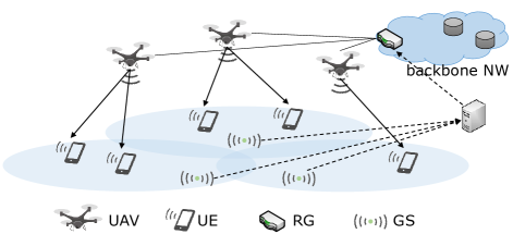
Figure 1: Illustration of UAV network model.

We now describe our model in detail. Table I summarizes the notations used in this paper. We assume that time is slotted as $t\in\{0,1,\dots\}\triangleq\mathbb{Z}_{+}$. Each time slot corresponds to the time at which the UAV positions are updated. We assume that the UAVs can move anywhere in a certain closed convex set $\Omega_{3}\subset\mathbb{R}^{2}\times\mathbb{R}_{+}$ where $\mathbb{R}_{+}=[0,\infty)$ and that the UEs are in a closed convex set $\Omega_{2}\subseteq\mathcal{P}(\Omega_{3})$ on the ground. Here, $\mathcal{P}:\mathbb{R}^{3}\to\mathbb{R}^{2}$ represents the projection from the 3D space to the plane (ground). Let $\mbox{\boldmath$u$}_{i}(t)=[u_{i0}(t),u_{i1}(t),u_{i2}(t)]^{\top}\in\Omega_{3}$ ($i\in\{1,\dots,U\}\triangleq\mathcal{U}$) denote the position of the $i$-th UAV at time $t\in\mathbb{Z}_{+}$. Here, $U$ denotes the total number of UAVs. We also write $\mbox{\boldmath$u$}(t)=[\mbox{\boldmath$u$}^{\top}_{1}(t),\dots,\mbox{\boldmath$u$}^{\top}_{U}(t)]^{\top}\in(\Omega_{3})^{U}$. Furthermore, we assume that the UEs are distributed according to a certain (inhomogeneous) spatial point process with an intensity function $\lambda(\mbox{\boldmath$y$})~{}(\mbox{\boldmath$y$}\in\Omega_{2})$. Although $\lambda(\cdot)$ depends on $t$ due to the dynamics of UEs, we omit the index for simplicity.

Next, we describe the activities of GSs. Let $\mbox{\boldmath$g$}_{n}\in\Omega_{2}~{}(n=1,\dots,N)$ denote the positions of GSs. Here, $N$ represents the total number of the GSs. The GSs are assumed to be capable of detecting and estimating the number of UEs around them by sensing and report their sensing results periodically at time $T_{k}\triangleq kT~{}(k\in\mathbb{Z}_{+})$. Here, $T$ denotes the sensing period and is assumed to be larger than UAVs’ update interval (i.e., $T\gg 1$) due to the computational time of sensing or crowd density estimation. Furthermore, let $x_{n}(T_{k})\in\mathbb{R}_{+}~{}(n=1,\dots,N)$ denote the sensing result reported from the $n$-th GS at time $T_{k}$, i.e., the (average) expected number of UEs per unit space in the neighborhood of $\mbox{\boldmath$g$}_{n}$. Thus, it can be regarded as an observation of $\lambda(\mbox{\boldmath$g$}_{n})$ at time $T_{k}$. We also express $\mbox{\boldmath$x$}(T_{k})=[x_{1}(T_{k}),\dots,x_{N}(T_{k})]^{\top}\in(\mathbb{R}_{+})^{N}$. Using $\mbox{\boldmath$x$}(T_{k})$, the crowd density estimation part infers the entire intensity function as $\widetilde{\lambda}_{k}(\mbox{\boldmath$y$})$ ($\mbox{\boldmath$y$}\in\Omega_{2}$). Note that we can easily consider the scenario where UAVs are equipped with sensors by taking into account sensing results at $\mbox{\boldmath$u$}_{i}(t)$’s. However, in this study, we assume that only GSs can perform sensing, for simplicity.

TABLE I: List of Notations

$\mbox{\boldmath$u$}_{i}(t)$, $\mbox{\boldmath$u$}(t)$	positions of $i$-th UAV and all UAVs at time $t$
$U$	total number of UAVs
$\mbox{\boldmath$g$}_{n}$	position of $n$-th GS
$N$	total number of GSs
$\lambda(\mbox{\boldmath$y$})$, $\widetilde{\lambda}(\mbox{\boldmath$y$})$	true and estimated intensity of UEs at $y$
$T$, $T_{k}$	sensing period and $k$-th sensing time
$x_{n}(T_{k})$, $\mbox{\boldmath$x$}(T_{k})$	sensing result at time $T_{k}$ from $n$-th or all GSs
$\theta_{i,y}(t)$	elevation angle from $y$ to $i$-th UAV at time $t$
$d_{i,y}$(t)	distance between $i$-th UAV and UE at $y$ at time $t$
$\mathcal{V}_{i}(\mbox{\boldmath$u$})$	UAV cell of $i$-th UAV
$\mathcal{N}_{i}(t)$	neighborhood of $i$-th UAV
$h_{i,y}(t)$	fading gain corresponding to $i$-th UAV and UE at $y$
$I_{i,y}(t)$	interference at UE at $y$ served by $i$-th UAV
$\sigma$	normalized thermal noise power
$\Theta$	SINR threshold

III-B Channel modeling and UAV-cell definition

We consider the following radio propagation model for UAV–UE channels. Due to the blockage effect in the A2G link, the link conditions can be divided into LoS and non-LoS (NLoS) conditions. We adopt a probabilistic LoS model similar to that in [5, 23], wherein a link condition ($\mathrm{L}:\mathrm{LoS}$, $\mathrm{N}:\mathrm{NLoS}$) is determined by the following probability:

$$\mathsf{P}(\mathrm{L};\theta_{i,y}(t)) ={1\over 1+b_{1}\exp(-b_{0}({180\over\pi}\theta_{i,y}(t)-b_{1}))},$$ (1)

$$\mathsf{P}(\mathrm{N};\theta_{i,y}(t)) =1-\mathsf{P}(\mathrm{L};\theta_{i,y}(t)),$$ (2)

where $b_{0}$ and $b_{1}$ are constants dependent on the environments (e.g., urban and rural) and are provided in [5], and $\theta_{i,y}(t)\in[0,\pi/2]$ is the elevation angle from a UE at $\mbox{\boldmath$y$}\in\Omega_{2}$ to the $i$-th UAV. Thus, if we denote $d_{i,y}(t)$ as the distance between the $i$-th UAV and a UE at $y$, $\theta_{i,y}(t)=\sin^{-1}(u_{i2}(t)/d_{i,y}(t))$. For simplicity, we assume that all the UAVs and UEs are equipped with omni-directional antennas. Although the channel condition is spatially and temporally correlated in general, for simplicity, we assume that they are independently determined at each time and position. We assume a distance-dependent path-loss model [23, 24] such that, for a distance $d$,

$$\ell_{q}(d)=\beta_{q}(\varepsilon_{0}+d)^{-\alpha_{q}}\quad\mbox{for $q\in\{\mathrm{L},\mathrm{N}\}$},$$

where $\alpha_{q}>2$ is a path-loss exponent, $\varepsilon_{0}>0$ denotes a constant to avoid a singularity at $d=0$, and $\beta_{q}>0$ is a constant that depends on the environment. Furthermore, we model the small-scale fading effect in UAV-UE channels with the independent Nakagami-$m$ fading similar to that in [24]. Let $h_{i,y}(t)$ denote the small-scale fading gain corresponding to the channel between the $i$-th UAV and a UE at $y$. Then, $h_{i,y}(t)$ is distributed according to the normalized gamma distribution with a parameter $m_{q}$ $(q\in\{\mathrm{L},\mathrm{N}\})$. For simplicity, we assume $m_{q}$ to be an integer throughout this paper. In addition, we omit the effects of shadowing and Doppler shift for mathematical tractability. The transmission power of each UAV is identical and is assumed to be normalized to one.

We next define the serving area of each UAV, i.e., a UAV-cell. In this paper, we assume that each UAV has a capacity sufficient for serving UEs. Moreover, each UE is assumed to associate with the UAV that provides the strongest average signal power. By definition, the average signal power from the $i$-th UAV to a UE at $y$ is expressed as

$$S_{i,y}(t)=\sum_{q\in\{\mathrm{L},\mathrm{N}\}}\mathsf{P}(q;\theta_{i,y}(t))\ell_{q}(d_{i,y}(t)).$$ (3)

The UAV-cell is then defined as a signal-weighted Voronoi cell, i.e., for the $i$-th UAV,

$$\mathcal{V}_{i}(\mbox{\boldmath$u$}(t))=\left\{\mbox{\boldmath$y$}\in\Omega_{2}\mid S_{i,y}(t)\geq S_{j,y}(t),\forall j\in\mathcal{U}\backslash\{i\}\right\}.$$ (4)

From this expression, we can construct an associated signal-weighted Delaunay graph $\mathcal{G}(t)$ by choosing the set of vertices as $\mathcal{U}$ and the set of edges as pairs of UAVs whose signal-weighted Voronoi cells are adjacent. Let $\mathcal{N}_{i}(t)$ denote the set of neighboring UAVs of the $i$-th UAV on the graph $\mathcal{G}(t)$. We assume that the $i$-th UAV can communicate with only $\mathcal{N}_{i}(t)$ in our distributed collaborative deployment method.

III-C Problem description

In this paper, we consider the total coverage of UEs, i.e., the total expected number of covered UEs, as the performance metric of UAV deployment. We assume that a UE is covered if the SINR at the UE exceeds a threshold $\Theta$. By considering a random channel condition and fading, the coverage probability of a UE at $y$ served by the $i$-th UAV is expressed as

$$C_{i,y}(\mbox{\boldmath$u$}(t)):=C_{i,y}(\mbox{\boldmath$u$}(t);\Theta)=\mathsf{P}(\mathsf{SINR}_{i,y}(t)>\Theta).$$ (5)

Here, $\mathsf{SINR}_{i,y}(t)$ is expressed as

$$\mathsf{SINR}_{i,y}(t)={h_{i,y}(t)\ell_{q}(d_{i,y}(t))\over I_{i,y}(t)+\sigma},$$ (6)

where $I_{i,y}(t)$ is the total interference power defined as

$$I_{i,y}(t)=\sum_{j\in\mathcal{U}\backslash\{i\}}h_{j,y}(t)\ell_{q}(d_{i,y}(t)),$$ (7)

and $\sigma$ denotes the thermal noise power and is assumed to be constant. By considering the coverage probability, we can characterize the communication quality of UEs more flexibly than the existing performance metrics based on mean path-loss [4, 15] or average SINR [7, 21]. By taking the expectation of the number of covered UEs on $\Omega_{2}$ and applying Campbell’s theorem [26], the total coverage can be expressed as

$$\int_{\Omega_{2}}\mathbb{E}[\mathbbold{1}(\mbox{UE at $\mbox{\boldmath$y$}$ is covered})]\lambda(\mbox{\boldmath$y$})\mathrm{d}\mbox{\boldmath$y$}$$

$$~{}~{}~{}~{}=\sum_{i\in\mathcal{U}}\int_{\mathcal{V}_{i}(\mbox{\boldmath$u$})}C_{i,y}(\mbox{\boldmath$u$})\lambda(\mbox{\boldmath$y$})\mathrm{d}\mbox{\boldmath$y$},$$ (8)

where $\mathbbold{1}(\cdot)$ denotes the indicator function.

We are now prepared to state our optimization problem. Our objective is to determine an optimal 3D deployment of UAVs that maximizes (8) in a distributed manner. Since the true intensity $\lambda(\mbox{\boldmath$y$})$ cannot be obtained in general, we use an estimated intensity for the deployment optimization instead.

Problem 1

Assume that i) each UAV $i$ $(i\in\mathcal{U})$ can communicate only with its neighborhood $\mathcal{N}_{i}(t)$ on $\mathcal{G}(t)$ and ii) the estimated intensity at $T_{k}$ ($k\in\mathbb{Z}_{+}$) based on sensing result $\mbox{\boldmath$x$}(T_{k})$ is given by $\widetilde{\lambda}_{k}(\mbox{\boldmath$y$})$. For each sensing period $k$, determine the optimal UAV deployment $\mbox{\boldmath$u$}\in(\Omega_{3})^{U}$ that maximizes the estimated total coverage $F(\mbox{\boldmath$u$}\mid\mbox{\boldmath$x$}(T_{k}))$ defined as

$$F(\mbox{\boldmath$u$}\mid\mbox{\boldmath$x$}(T_{k})) =\sum_{i\in\mathcal{U}}\int_{\mathcal{V}_{i}(\mbox{\boldmath$u$})}C_{i,y}(\mbox{\boldmath$u$})\widetilde{\lambda}_{k}(\mbox{\boldmath$y$})\mathrm{d}\mbox{\boldmath$y$}.$$ (9)

IV Distributed UAV 3D Deployment Method

In this section, we present the distributed collaborative UAV 3D deployment method. Our method mainly consists of two parts: i) sensing-aided crowd density estimation; and ii) distributed push-sum algorithm. At each sensing time $T_{k}$, GSs send $\mbox{\boldmath$x$}(T_{k})$ to a central server. The crowd estimation part then estimates $\lambda(\mbox{\boldmath$y$})$. During the $k$-th sensing period, UAVs update their 3D positions by using $\widetilde{\lambda}_{k}(\mbox{\boldmath$y$})$ via the distributed push-sum algorithm, which is aimed at solving Problem 1.

This section is organized as follows. We first analyze our performance metrics, namely the coverage probability and total coverage in Section IV-A. We then describe the crowd density estimation part in Section IV-B and present the distributed push-sum algorithm part in Section IV-C. Finally, we prove the convergence of the distributed algorithm in Section IV-D.

IV-A Coverage analysis

Since our distributed optimization method is gradient-based, we analyze the total coverage and derive its gradient in this section. We omit the index $t$ in this section because a fixed time is being considered. We start by deriving the theoretical expression of the coverage probability of UEs. By using the expressions of (5) and (6), we can obtain the following result. A sketch of the proof is provided in Appendix A.

Lemma 1

If the deployment of UAVs is $\mbox{\boldmath$u$}\in(\Omega_{3})^{U}$, the coverage probability $C_{i,y}(\mbox{\boldmath$u$})$ can be approximated by

$$C_{i,y}(\mbox{\boldmath$u$})\approx\widetilde{C}_{i,y}(\mbox{\boldmath$u$}) \triangleq\sum_{q_{0}\in\{\mathrm{L},\mathrm{N}\}}\mathsf{P}(q_{0};\theta_{i,y})\sum_{k=1}^{m_{q_{0}}}(-1)^{k+1}$$

$$\times{m_{q}\choose k}e^{-k\sigma\gamma_{q_{0},i,y}}\mathcal{L}_{I_{i,y}}(k\gamma_{q_{0},i,y}),$$ (10)

where $\gamma_{q,i,y}={\eta_{q}\Theta\over\ell_{q}(d_{i,y})}$ with $\eta_{q}=m_{q}(m_{q}!)^{-{1\over m_{q}}}$ for $q\in\{\mathrm{L},\mathrm{N}\}$, and $\mathcal{L}_{I_{i,y}}(s)$ is given by

$$\mathcal{L}_{I_{i,y}}(s)=\!\!\prod_{j\in\mathcal{U}\backslash\{i\}}\!\sum_{q_{j}\in\{\mathrm{N},\mathrm{L}\}}\!\!\!\mathsf{P}(q_{j};\theta_{j,y})\left(1+{s\ell_{q_{j}}(d_{j,y})\over m_{q_{j}}}\right)^{-m_{q_{j}}}\!\!\!\!\!\!\!\!.$$

On the basis of Lemma 1, we aim to solve Problem 1 through $\widetilde{C}_{i,y}(\mbox{\boldmath$u$})$ in what follows. In other words, we replace $C_{i,y}(\mbox{\boldmath$u$})$ in the objective function in (9) by $\widetilde{C}_{i,y}(\mbox{\boldmath$u$})$ and consider the optimization problem of the following function:

$$\widetilde{F}(\mbox{\boldmath$u$}\mid\mbox{\boldmath$x$}(T_{k})) =\sum_{i\in\mathcal{U}}\int_{\mathcal{V}_{i}(\mbox{\boldmath$u$})}\widetilde{C}_{i,y}(\mbox{\boldmath$u$})\widetilde{\lambda}_{k}(\mbox{\boldmath$y$})\mathrm{d}\mbox{\boldmath$y$}.$$ (11)

Furthermore, from (10), we can calculate the derivatives of $\widetilde{C}_{i,y}(\mbox{\boldmath$u$})$ with respect to $\mbox{\boldmath$u$}_{j}$, i.e.,

$$\widetilde{\mbox{\boldmath$c$}}^{j}_{i,y}(\mbox{\boldmath$u$})\triangleq{\mathrm{d}\over\mathrm{d}\mbox{\boldmath$u$}_{j}}\widetilde{C}_{i,y}(\mbox{\boldmath$u$}),\qquad i,j\in\mathcal{U}.\vspace{-1mm}$$

Since we can conveniently obtain $\widetilde{\mbox{\boldmath$c$}}^{j}_{i,y}(\mbox{\boldmath$u$})$ from Lemma 1, we omit their explicit expressions due to space limitations.

Next, we demonstrate that the derivative of $\widetilde{F}(\mbox{\boldmath$u$}\mid\mbox{\boldmath$x$})$ with respect to $\mbox{\boldmath$u$}_{j}$ can be approximated through $\widetilde{\mbox{\boldmath$c$}}_{i,y}^{j}(\mbox{\boldmath$u$})$. A sketch of the proof is provided in Appendix B. In what follows, we simply write $\widetilde{F}(\mbox{\boldmath$u$}):=\widetilde{F}(\mbox{\boldmath$u$}\mid\mbox{\boldmath$x$})$ for readability.

Lemma 2

If the estimated intensity function is $\widetilde{\lambda}(\mbox{\boldmath$y$})$ ($\mbox{\boldmath$y$}\in\Omega_{2}$),

$${\mathrm{d}\widetilde{F}(\mbox{\boldmath$u$})\over\mathrm{d}\mbox{\boldmath$u$}_{j}}\approx\sum_{i\in\mathcal{U}}\int_{\mathcal{V}_{i}(\mbox{\boldmath$u$})}\widetilde{\mbox{\boldmath$c$}}_{i,y}^{j}(\mbox{\boldmath$u$})\widetilde{\lambda}(\mbox{\boldmath$y$})\mathrm{d}\mbox{\boldmath$y$},\quad\mbox{$j\in\mathcal{U}$}.$$ (12)

According to Lemma 2, the gradient of $\widetilde{F}(\mbox{\boldmath$u$})$ exhibits the following useful (approximate) separation property, which enables us to optimize $\widetilde{F}(\mbox{\boldmath$u$})$ in a distributed manner:

$$\nabla\widetilde{F}(\mbox{\boldmath$u$}) \approx\sum_{i\in\mathcal{U}}\widehat{\mbox{\boldmath$f$}}_{i}(\mbox{\boldmath$u$}),$$ (13)

where, for $i\in\mathcal{U}$,

$$\widehat{\mbox{\boldmath$f$}}_{i}(\mbox{\boldmath$u$}) \triangleq\left[\int_{\mathcal{V}_{i}(\mbox{\boldmath$u$})}\widetilde{\mbox{\boldmath$c$}}_{i,y}^{j}(\mbox{\boldmath$u$})\widetilde{\lambda}(\mbox{\boldmath$y$})\mathrm{d}\mbox{\boldmath$y$}\right]^{\top}_{j\in\mathcal{U}}$$

$$=\int_{\mathcal{V}_{i}(\mbox{\boldmath$u$})}\nabla\widetilde{C}_{i,y}(\mbox{\boldmath$u$})\widetilde{\lambda}(\mbox{\boldmath$y$})\mathrm{d}\mbox{\boldmath$y$}.$$ (14)

The above relationship indicates that there exists $\widehat{F}(\mbox{\boldmath$u$})$ such that $\nabla\widehat{F}(\mbox{\boldmath$u$})=\sum_{i\in\mathcal{U}}\widehat{\mbox{\boldmath$f$}}_{i}(\mbox{\boldmath$u$})$ and $\widetilde{F}(\mbox{\boldmath$u$})\approx\widehat{F}(\mbox{\boldmath$u$})$.

IV-B Crowd density estimation

We next describe the crowd density estimation. The aim of this part is to estimate the intensity function from the sensing results at sensing time $T_{k}$ ($k\in\mathbb{Z}_{+}$), i.e., to obtain $\widetilde{\lambda}_{k}(\mbox{\boldmath$y$})$ from $\mbox{\boldmath$x$}(T_{k})$. Typically, the density of UEs is spatially correlated owing to geographical factors, such as roads and attractions. Thus, by modeling this spatial correlation, we infer the entire intensity function with a limited number of GSs.

For a fixed sensing time, we consider a spatial Gaussian process (GP) prior $\mathrm{GP}(\mu,k_{0}(\mbox{\boldmath$y$},\mbox{\boldmath$y$}^{\prime}))$ $(\mbox{\boldmath$y$},\mbox{\boldmath$y$}^{\prime}\in\mathbb{R}^{2})$ for $\lambda(\mbox{\boldmath$y$})$. Here, the constant $\mu$ expresses the mean of $\mathrm{GP}$ and corresponds to a prior expectation of $\lambda(\mbox{\boldmath$y$})$. Meanwhile, $k_{0}(\mbox{\boldmath$y$},\mbox{\boldmath$y$}^{\prime})$ is the kernel function of $\mathrm{GP}$ and represents the spatial correlation of $\lambda(\mbox{\boldmath$y$})$. In this paper, we adopt a well-accepted Gaussian kernel:

$$k_{0}(\mbox{\boldmath$y$},\mbox{\boldmath$y$}^{\prime})=A_{0}\exp\left(-{\|\mbox{\boldmath$y$}-\mbox{\boldmath$y$}^{\prime}\|^{2}\over A_{1}}\right),\qquad\mbox{\boldmath$y$},\mbox{\boldmath$y$}^{\prime}\in\mathbb{R}^{2},$$ (15)

where $\|\cdot\|$ denotes the Euclidean norm and $A_{0}$ and $A_{1}$ are constants. We assume that the parameters of GP (i.e., $\mu$, $A_{0}$, and $A_{1}$) are obtained from statistical data. GPs are widely used in modeling various spatial data [27] ranging from geology to environmental sciences. According to an established property of a GP, if we regard observations $\mbox{\boldmath$x$}(T_{k})$ as realizations of $\lambda(\mbox{\boldmath$g$}_{n})$ ($n=1,\dots,N$) at $T_{k}$, they are distributed with a multivariate Gaussian distribution. Furthermore, the posterior distribution of $\lambda(\mbox{\boldmath$y$})$ given $\mbox{\boldmath$x$}(T_{k})$ also becomes a Gaussian (e.g., [27]): as follows:

$$\lambda(\mbox{\boldmath$y$})\mid\mbox{\boldmath$x$}(T_{k}),\{\mbox{\boldmath$g$}_{n};n=1,\dots,N\}$$

$$\quad\sim\mathcal{N}(\mu_{y}(\mbox{\boldmath$x$}(T_{k})),k_{0}(\mbox{\boldmath$y$},\mbox{\boldmath$y$})-\mbox{\boldmath$k$}_{y}^{\top}\mbox{\boldmath$K$}^{-1}_{\!g}\mbox{\boldmath$k$}_{y}),$$ (16)

where

$$\mu_{y}(\mbox{\boldmath$x$}(T_{k})) =\mu+\mbox{\boldmath$k$}_{y}^{\top}\mbox{\boldmath$K$}_{\!g}^{-1}(\mbox{\boldmath$x$}(T_{k})-\mu\mbox{\boldmath$e$}),$$ (17)

$$\mbox{\boldmath$k$}_{y} =[k_{0}(\mbox{\boldmath$g$}_{1},\mbox{\boldmath$y$}),\dots,k_{0}(\mbox{\boldmath$g$}_{N},\mbox{\boldmath$y$})]^{\top},$$

$$[K_{\!g}]_{n,n^{\prime}} =k_{0}(\mbox{\boldmath$g$}_{n},\mbox{\boldmath$g$}_{n}^{\prime}),\qquad n,n^{\prime}=1,\dots,N,$$

and $e$ denotes a vector of ones with an appropriate dimension. As a result, UAVs can estimate the entire intensity from the observations $\mbox{\boldmath$x$}(T_{k})$ by setting

$$\widetilde{\lambda}_{k}(\mbox{\boldmath$y$})=\mu_{y}(\mbox{\boldmath$x$}(T_{k})),\qquad\mbox{\boldmath$y$}\in\Omega_{2}.$$ (18)

By substituting (18) into (11), $\widetilde{F}(\mbox{\boldmath$u$}\mid\mbox{\boldmath$x$}(T_{k}))$ in (11) is now rewritten as

$$\widetilde{F}(\mbox{\boldmath$u$}\mid\mbox{\boldmath$x$}(T_{k})) =\sum_{i\in\mathcal{U}}\int_{\mathcal{V}_{i}(\mbox{\boldmath$u$})}\widetilde{C}_{i,y}(\mbox{\boldmath$u$})\mu_{y}(\mbox{\boldmath$x$}(T_{k}))\mathrm{d}\mbox{\boldmath$y$}.$$ (19)

IV-C Distributed push-sum algorithm

In this section, we describe the distributed push-sum algorithm. In this part, UAVs update their positions and maximize (19) in a distributed manner. Our objective function (19) depends on the positions of all the UAVs. Therefore, it is not trivial to solve the problem in a distributed manner. However, the useful separation property of $\nabla\widetilde{F}(\mbox{\boldmath$u$})$ in (13) enables us to apply a distributed push-sum framework. This framework was first proposed by [12] for average computation. It was recently extended to a time varying network by [28], and to a non-convex optimization problem by Tatarenko and Touri [13].

To state the algorithm, we first introduce an extension $\widehat{\mbox{\boldmath$f$}}^{\ast}_{i}$ of $\widehat{\mbox{\boldmath$f$}}_{i}$ that is defined on $(\mathbb{R}^{3})^{U}$ and satisfies

$$\widehat{\mbox{\boldmath$f$}}^{\ast}_{i}(\mbox{\boldmath$u$})=\left\{\begin{array}[]{ll}\widehat{\mbox{\boldmath$f$}}_{i}(\mbox{\boldmath$u$}),&\mbox{\boldmath$u$}\in(\Omega_{3})^{U},\\ J\breve{\mbox{\boldmath$u$}},&\mbox{\boldmath$u$}\in\overline{D},\\ \end{array}\right.$$ (20)

where $\overline{D}$ denotes the complement of an open set $D\subset(\mathbb{R}^{3})^{U}$ disjoint with $(\Omega_{3})^{U}$. In addition, $J>0$ is a constant and $\breve{\mbox{\boldmath$u$}}$ denotes a unit vector directed from $u$ toward its closest point on the boundary of $(\Omega_{3})^{U}$. In the next section, we prove the existence of $\widehat{\mbox{\boldmath$f$}}^{\ast}_{i}$ that satisfies several conditions required for the convergence of the distributed push-sum algorithm.

Algorithm 1 Distributed push-sum algorithm

1:  Initialize: $\mbox{\boldmath$u$}^{[i]}(0)$, $\mbox{\boldmath$w$}^{[i]}(0)$, $\mbox{\boldmath$\xi$}^{[i]}(0)$ and $\phi^{[i]}(0)$;

2:  for $t=0,1,\dots$ do

3:     for each UAV $i$ do

4:        Update $\mathcal{N}_{i}$ and $\mathcal{V}_{i}(\mbox{\boldmath$u$})$ of UAV $i$;

5:        for each neighboring UAV $j$ do

6:            Send $\mbox{\boldmath$\xi$}^{[i]}(t)$ and $\phi^{[i]}(t)$ to UAV $j$; andReceive $\mbox{\boldmath$\xi$}^{[j]}(t)$ and $\phi^{[j]}(t)$ from UAV $j$;

7:        end for

8:         Update $\mbox{\boldmath$u$}^{[i]}(t)$, $\mbox{\boldmath$w$}^{[i]}(t)$, $\mbox{\boldmath$\xi$}^{[i]}(t)$ and $\phi^{[i]}(t)$ by (21);

9:         Update position of UAV $i$: $\mbox{\boldmath$u$}_{i}(t+1):=\mbox{\boldmath$u$}_{i}^{[i]}(t+1)$;

10:     end for

11:  end for

We now describe the algorithm in detail. The pseudo-code is given in Algorithm 1. Each UAV $i$ (i.e., the $i$-th UAV) maintains a $3U$-dimensional vector $\mbox{\boldmath$u$}^{[i]}(t)\in(\mathbb{R}^{3})^{U}$, which represents the pseudo positions of the UAVs. Here, pseudo indicates that this location information is local for the UAV $i$ and does not always represent the exact positions of the other UAVs (only $\mbox{\boldmath$u$}^{[i]}_{i}(t)$ expresses the exact position of the UAV $i$). This is because each UAV can only communicate with its neighboring UAVs. They also maintain auxiliary $3U$-dimensional vectors $\mbox{\boldmath$w$}^{[i]}(t)$, and $\mbox{\boldmath$\xi$}^{[i]}(t)$, and a scholar variable $\phi^{[i]}(t)$. In each time step, each UAV $i$ updates its local variables according to the following rules:

$$\mbox{\boldmath$w$}^{[i]}(t+1) :=\!\!\!\sum_{j\in\mathcal{N}_{i}(t)}{\mbox{\boldmath$\xi$}^{[j]}(t)\over d_{j}(t)},~{}\phi^{[i]}(t+1):=\!\!\!\sum_{j\in\mathcal{N}_{i}(t)}{\phi^{[j]}(t)\over d_{j}(t)},$$

$$\mbox{\boldmath$u$}^{[i]}(t+1) :={\mbox{\boldmath$w$}^{[i]}(t+1)\over\phi^{[i]}(t+1)},$$ (21)

$$\mbox{\boldmath$\xi$}^{[i]}(t+1) :=\mbox{\boldmath$w$}^{[i]}(t+1)$$

$$~{}~{}~{}+a(t+1)(\widehat{\mbox{\boldmath$f$}}^{\ast}_{i}(\mbox{\boldmath$u$}^{[i]}(t+1))+\mbox{\boldmath$\kappa$}^{[i]}(t+1)),$$

where $\mbox{\boldmath$\kappa$}^{[i]}(t)\in(\mathbb{R}^{3})^{U}$ are i.i.d. random vectors whose entries are independent random variables with zero mean and unit variance for all $t\in\mathbb{Z}_{+}$. Moreover, $\{a(t)\}$ is a positive non-increasing step-size sequence such that $a(t)=O({1\over t^{\nu}})$ $(\nu\in({1\over 2},1))$ and $d_{i}(t)$ is the node degree of the UAV $i$ on $\mathcal{G}(t)$.

The update rules in (21) can be interpreted simply as follows. Each UAV aims to reach a consensus among the UAVs by exchanging its local information with its neighbors and calculating their weighted sum. Furthermore, by combining with a gradient descent based on its local information (i.e., $\widehat{\mbox{\boldmath$f$}}^{\ast}_{i}(\mbox{\boldmath$u$})$), the consensus point is steered towards a critical point of the objective function. In addition, the random perturbation $\mbox{\boldmath$\kappa$}^{[i]}(t)$ ensures the convergence to a local optimum [13].

IV-D Proof of convergence

In this section, we prove that the distributed push-sum algorithm given in (21) converges to a local optimum of the objective function among all the UAVs by employing the framework in [13]. To do this, we first prove the existence of an extension $\widehat{\mbox{\boldmath$f$}}^{\ast}_{i}(\mbox{\boldmath$u$})$ $(i\in\mathcal{U})$ in (20) and the antiderivative $\widehat{F}^{\ast}(\mbox{\boldmath$u$})$ of $\sum_{i\in\mathcal{U}}\widehat{\mbox{\boldmath$f$}}^{\ast}_{i}(\mbox{\boldmath$u$})$ satisfying several regularity properties.

Lemma 3

There exist functions $\widehat{\mbox{\boldmath$f$}}^{\ast}_{i}(\mbox{\boldmath$u$})$ $(i\in\mathcal{U})$ and $\widehat{F}^{\ast}(\mbox{\boldmath$u$})$ on $(\mathbb{R}^{3})^{U}$ such that $\widehat{\mbox{\boldmath$f$}}^{\ast}_{i}(\mbox{\boldmath$u$})=\widehat{\mbox{\boldmath$f$}}_{i}(\mbox{\boldmath$u$})$ and $\widehat{F}^{\ast}(\mbox{\boldmath$u$})\approx\widetilde{F}(\mbox{\boldmath$u$})$ in $(\Omega^{3})^{U}$ and

1. $\widehat{\mbox{\boldmath$f$}}^{\ast}_{i}(\mbox{\boldmath$u$})$ is bounded on $(\mathbb{R}^{3})^{U}$ for all $i\in\cal U$;

2. $\widehat{\mbox{\boldmath$f$}}^{\ast}_{i}(\mbox{\boldmath$u$})$ is Lipchitz continuous on $(\mathbb{R}^{3})^{U}$ for all $i\in\cal U$;

3. $\nabla\widehat{F}^{\ast}(\mbox{\boldmath$u$})=\sum_{i\in\mathcal{U}}\widehat{\mbox{\boldmath$f$}}^{\ast}_{i}(\mbox{\boldmath$u$})$; and

4. $\lim_{\|\mbox{\boldmath$u$}\|\to\infty}\widehat{F}^{\ast}(\mbox{\boldmath$u$})=-\infty$.

Proof.

Due to space limitations, we provide only a summary of the proof. In what follows, we fix $i\in\mathcal{U}$ arbitrary. We can confirm that $\widetilde{\mbox{\boldmath$c$}}^{j}_{i,y}(\mbox{\boldmath$u$})$ $(j\in\mathcal{U})$ are all bounded on $(\Omega_{3})^{U}$. We can also confirm that $\mbox{\boldmath$\mu$}_{y}(\mbox{\boldmath$x$})$ is bounded on $\mbox{\boldmath$y$}\in\Omega_{2}$ (see (17)) and $\mathcal{V}_{i}(\mbox{\boldmath$u$})$ is a closed set. It then follows from (14) and (18) that $\widehat{\mbox{\boldmath$f$}}_{i}(\mbox{\boldmath$u$})$ is bounded on $(\Omega_{3})^{U}$. Furthermore, we can prove that $\widehat{\mbox{\boldmath$f$}}_{i}(\mbox{\boldmath$u$})$ is continuously differentiable in $(\Omega_{3})^{U}$ and the derivatives are bounded on $(\Omega_{3})^{U}$, which indicates that $\widehat{\mbox{\boldmath$f$}}_{i}(\mbox{\boldmath$u$})$ is Lipschitz continuous with a certain Lipschitz constant $L_{0}$. Thus, if we extend the domain of $\widehat{\mbox{\boldmath$f$}}_{i}(\mbox{\boldmath$u$})$ to $(\Omega_{3})^{U}\cup\overline{D}$ similarly as in (20), $\widehat{\mbox{\boldmath$f$}}_{i}(\mbox{\boldmath$u$})$ is bounded and Lipschitz continuous with $L_{0}$ on $(\Omega_{3})^{U}\cup\overline{D}$. It thus follows from Tietze’s extension theorem that there exists a bounded and Lipschitz continuous function $\widehat{\mbox{\boldmath$f$}}^{\ast}_{i}(\mbox{\boldmath$u$})$ on $(\mathbb{R}^{3})^{U}$ with $L_{0}$ such that $\widehat{\mbox{\boldmath$f$}}^{\ast}_{i}(\mbox{\boldmath$u$})=\widehat{\mbox{\boldmath$f$}}_{i}(\mbox{\boldmath$u$})$ in $(\Omega_{3})^{U}\cup\overline{D}$. These results indicate that the statements (i) and (ii) hold. Furthermore, by using $\sum_{i\in\mathcal{U}}\widehat{\mbox{\boldmath$f$}}^{\ast}_{i}(\mbox{\boldmath$u$})$ and (13), we can construct a continuously differentiable function $\widehat{F}^{\ast}(\mbox{\boldmath$u$})$ on $(\mathbb{R}^{3})^{U}$ such that $\widehat{F}^{\ast}(\mbox{\boldmath$u$})\approx\widetilde{F}(\mbox{\boldmath$u$})$ in $(\Omega^{3})^{U}$ and the statements (iii) and (iv) hold, which completes the proof. ∎

Combining Lemma 3 with the facts that $\widehat{\mbox{\boldmath$f$}}_{i}(\mbox{\boldmath$u$})$ is differentiable in $(\Omega_{3})^{U}$ and the sequence $\{\mathcal{G}(t)\}$ is strongly connected, i.e., the union of their edge sets is strongly connected, we can apply Theorem 5 in [13] to $\widehat{F}^{\ast}(\mbox{\boldmath$u$})\ (\approx\widetilde{F}(\mbox{\boldmath$u$}))$ and $\widehat{\mbox{\boldmath$f$}}^{\ast}_{i}(\mbox{\boldmath$u$})$ in Lemma 3 and prove the convergence of the algorithm.

Theorem 1

Each $\mbox{\boldmath$u$}^{[i]}(t)$ $(i\in\mathcal{U})$ and the average state variable ${1\over U}\sum_{i=1}^{U}\mbox{\boldmath$\xi$}^{[i]}(t)$ in the distributed push-sum algorithm in (21) converge to a point in the set of local maxima of $\widehat{F}^{\ast}(\mbox{\boldmath$u$})$ from any initial state.

V Simulation Results

We evaluate our distributed 3D UAV deployment method by conducting numerical simulations. In each simulation, we assume that $U=9$ UAVs are deployed over a ($5000$ m)² area ($\Omega_{2}$) with a maximum altitude 1500 m. We adopted values similar to those in [25, 24] for the parameters of the channel model associated with the $\mathrm{LoS}$ and $\mathrm{NLoS}$ conditions. We also considered sub-urban, urban, and dense-urban scenarios by selecting the values of $b_{0}$ and $b_{1}$ presented in [4]. The other parameters are listed in Table II unless otherwise stated. In addition, we randomly generated spatially correlated intensity by the following procedure. We first divided the whole area into $50\times 50$ small grids, and then sampled the values of $\lambda(\mbox{\boldmath$y$})$ in each grid from a multivariate Gaussian distribution whose covariance matrix is determined by the kernel function in (15).

TABLE II: Simulation Parameters

Parameter	Value	Parameter	Value
$b_{0}$, $b_{1}$	0.16, 9.61 (urban)	$\beta_{\mathrm{L}}$, $\beta_{\mathrm{N}}$	0.092, 0.035
	0.43, 4.88 (sub urban)	$m_{\mathrm{L}}$, $m_{\mathrm{N}}$	3, 2
	0.11, 12.08 (dense urban)	$\alpha_{\mathrm{L}}$, $\alpha_{\mathrm{N}}$	2, 3
$\mu$	100 m-2	$\sigma$	$-70$ dBm
$A_{0}$, $A_{1}$	10, (500)2	length of area	5000 m
$\Theta$	0 dB	default altitude	200 m

V-A Effectiveness of distributed push sum algorithm

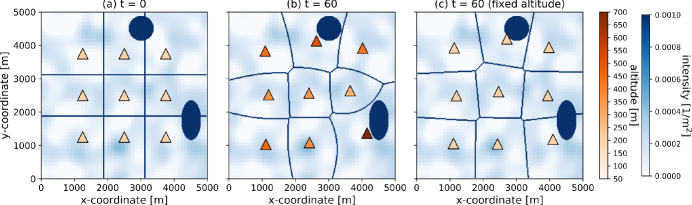
Figure 2: 3D UAV deployment in urban scenario (a) $t=0$ and (b) $t=60$, and (c) fixed altitude scenario $t=60$. Triangles represent horizontal positions of UAVs and their color depth represent altitudes. Depth of background color expresses intensity of UEs and dark ellipses represent artificially added hotspots.

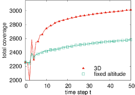
Figure 3: Comparison of process of total coverage with 3D deployment and fixed altitude scenarios.

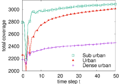
Figure 4: Comparison of process of total coverage with different scenarios.

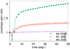
Figure 5: Comparison of process of ratio of coverages with different $\Theta$.

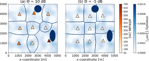
Figure 6: 3D UAV deployment in urban scenario at $t=60$.

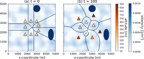
Figure 7: 3D UAV deployment starting from centered positions with $\Theta=0$ dB at (a) $t=0$ and (b) $t=100$.

We first focus on the performance of the distributed push-sum algorithm part and demonstrate its effectiveness. We also investigate the impacts of several parameters on the performance and the resulting UAV deployment. To achieve this, we focused on a sensing period, i.e., a fixed $T_{k}$, and assumed that all the UAVs knew the true $\lambda(\mbox{\boldmath$y$})$, i.e., $\lambda(\mbox{\boldmath$y$})\equiv\widetilde{\lambda}_{k}(\mbox{\boldmath$y$})$ ($\mbox{\boldmath$y$}\in\Omega_{2}$). We then set artificial hotspots, in which the intensity of UEs is $10\cdot\mu$ (see Fig. 3 (a)). In addition, the initial positions of the UAVs were uniformly arranged with the equal intervals.

Fig. 3 shows the 3D placement of the UAVs at $t=0,60$ in the urban scenario. We also plotted in Fig. 3 (c) the case where the altitudes of the UAVs were fixed at the default altitude by controlling only their horizontal movements. The triangles in the graphs express the positions of the UAVs, and their altitudes are represented by their color depth. Each cell corresponds to each UAV-cell. The background color depth expresses the intensity of UEs, and the dark ellipses correspond to the artificially added hotspots. We also illustrate the process of the total coverage (i.e., the objective function) in Fig. 3. Fig. 3 (a) and (b) reveal that the 3D positions of the UAVs and associated shapes of the UAV-cells dynamically adjusted to the hotspots so that each hotspot was fitted in a UAV-cell to avoid interference. As a result, the total coverage was significantly improved from the initial deployment (approximately 35 % higher). On the other hand, the total coverage was less improved in the fixed altitude scenario. Fig. 3 (b) also shows that the altitudes of the UAVs serving hotspots were higher than those of the other UAVs. Moreover, the altitudes of the UAVs changed more aggressively than their horizontal positions. This is because as the altitude of a UAV increases, the LoS probability increases, and thus the UAV-cell and the coverage probability also increase. These results indicate that the total coverage is more sensitive to the vertical movements of the UAVs than to their horizontal ones. Thus, their 3D position must be considered for an efficient UAV deployment optimization.

Fig. 5 shows the process of the total coverage in sub-urban, urban, and dense urban scenarios. Although the total coverage increased in all cases, their improvements varied depending on the scenarios. The reason for this can be considered as follows. Since the coverage area of a UAV is larger in the sub-urban scenario than the other scenarios [5, 4], the whole area was sufficiently covered even with an initial placement. Thus, the benefit of our method was smaller in the sub-urban scenario than the urban one. On the other hand, in the dense-urban scenario, ground UEs could not be covered by $U=9$ UAV-BSs due to the small coverage area.

We next investigate the impacts of the SINR threshold $\Theta$. To see the difference more clearly, we calculated the ratio of the total coverage at each step to that at $t=0$. Fig. 5 expresses the processes of the ratio with different $\Theta$. The graph shows that the improvement with higher $\Theta$ becomes larger, whereas that with $\Theta=-5$ dB was highly limited. This is because with low $\Theta$, the total coverage was already sufficient even in the initial step, and thus the objective function did not exhibit much potential for improvement. Meanwhile, when $\Theta=10$ dB, the total coverage became approximately two times of that in the initial step. This result indicates that our optimization method is highly efficient for a high SINR regime. We also illustrate the 3D deployment of the UAVs in Fig. 6 in each case. The deployment with $\Theta=10$ dB was similar to that with $\Theta=0$ dB, whereas the altitudes of the UAVs with $\Theta=-5$ dB were much lower than the other cases.

Finally, we demonstrate the impact of the initial positions of the UAVs. Fig. 7 shows the 3D deployment of the UAVs at $t=0,100$ when their initial positions were gathered at the center. The figures show that as the time elapsed, the positions of the UAVs adjusted to the hotspots and the UAVs maintained certain distances among themselves to reduce interference. In addition, the altitudes of the UAVs serving the hotspots became high again, whereas the resulting deployment was different from that in the previous scenario.

V-B Effect of crowd density estimation

We next focus on the effect of the crowd density estimation part. Unlike the previous scenario, we assumed that the intensity function is available only at randomly generated GSs (grids where GSs exist). The entire intensity was calculated by the crowd density estimation method described in Section IV-B. Since the number of GSs is likely to impact the performance, we evaluated it by considering the GS deployment ratio $r_{\mathrm{GS}}\in[0,1]$. This is defined as the ratio of the grids where GSs exist to the total grids. We regarded each grid as the sensing range of a GS and assumed that the intensity in each GS’s grid was obtained correctly. To evaluate the impact of $r_{\mathrm{GS}}$, we consider the coverage gain, which was calculated as the difference between the total coverage at $t=0$ and $30$. We first calculated the coverage gain in the case with complete information of true intensity, (i.e., $r_{\mathrm{GS}}=1$) as a baseline. We then calculated the ratio of the coverage gain with each $r_{\mathrm{GS}}$ to the baseline. Fig. 8 illustrates the result of the ratio of coverage gain. For each $r_{\mathrm{GS}}$, we generated 10 samples of the GS placement. The figure shows that as expected, as $r_{\mathrm{GS}}$ increases, the performance of of our method also increases. This is because the proposed algorithm optimizes the positions of UAVs by using $\widetilde{\lambda}(\mbox{\boldmath$y$})$ (see (11)). Thus, if the intensity function was incorrectly estimated, the proposed method failed to update the UAV placement effectively for improving the objective function. However, the simulation results demonstrate that even a small $r_{\mathrm{GS}}$ (e.g., $r_{\mathrm{GS}}=0.03$, 3 GS/km²) achieved 98% of the baseline in the urban scenario. This indicates that our method could improve the total coverage even with a limited number of GSs.

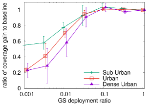
Figure 8: Ratio of coverage gain to baseline versus GS deployments ratio $r_{GS}$. Error bars represent 95 % confidence interval.

V-C Dynamic network scenario

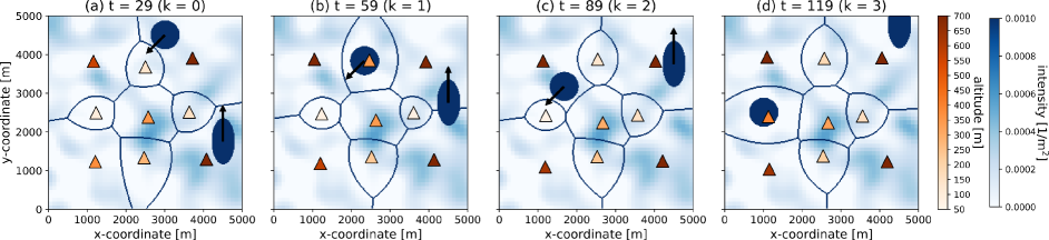
Figure 9: 3D UAV deployment process in dynamic network scenario at (a) $t=29~{}(k=0)$; (b) $t=59~{}(k=1)$; (c) $t=89~{}(k=2)$ and (d) $t=119~{}(k=3)$. Initial deployment of UAVs was the same as that in Fig. 3 (a). Hotspots are represented as dark ellipses, and arrows represent their moving directions.

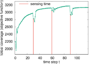
Figure 10: Process of total coverage. Vertical lines represent sensing times.

We next apply our algorithm to a more dynamic network, in which the positions of hotspots change dynamically. Unlike the previous examples, we consider multiple sensing periods and assume that hotspots move at each sensing time. We first artificially set hotspots on $\Omega_{2}$ similarly as those in Fig. 3. We then moved each of them in a predefined direction at $T_{k}$ $(k=1,2,3)$ with $T=30$. The initial deployment of UAVs $(T_{0}=0)$ was also the same as Fig. 3 (a). Fig. 9 illustrates the 3D deployment of UAVs at the end of each sensing period (e.g., (b) shows $t=59$, the end of the first sensing period ($k=1$)). We also show the process of the total coverage in Fig. 10. As the figures show, at each sensing time, the total coverage temporarily decreased due to the movement of the hotspots. However, as shown in Fig. 9, the UAVs adjusted their positions to the hotspot locations and successfully increased the total coverage. For example, in Fig. 9 (b) and (d), (i.e., $k=1,3$), the left hotspot moved to a position on the borders of UAV-cells. However, the UAVs changed their 3D positions and the shapes of the UAV-cells to reduce interference. Note that, at $t=59$ (b), the right hotspot is on the border of UAV cells. This is because our algorithm could not sufficiently optimize the UAV placement during a sensing period. However, the total coverage was successfully improved as shown in Fig. 10. Consequently, our method could respond to hotspots and provide coverage to UEs in a dynamic network in an on-demand manner.

VI Conclusion

In this paper, we proposed a distributed UAV-BS 3D deployment method for on-demand coverage. Since the specific positions of ground users may not be obtained in real networks, we proposed the sensing-aided crowd density estimation method. Furthermore, by adopting total coverage as the performance metric, we developed a push-sum-based distributed UAV 3D deployment algorithm. Several simulation results revealed that our method can improve the overall coverage of ground users with the aid of a limited number of sensors and can be applied to a dynamic network.

In our problem setting, we assumed that the UAVs exhibit identical transmission power. Thus, the joint optimization of 3D UAV deployment and energy consumption are topics for our future work. Furthermore, other physical constraints, such as the capacity of UAVs [7], and obstacle avoidance [21] should be considered while applying our method to a real network. Moreover, simulations considering more realistic user density, such as road constraints, remain for future work.

Appendix A: Proof of Lemma 1

By conditioning on the status of the desired channel between $\mbox{\boldmath$u$}_{i}$ and $y$, $C_{i,y}(\mbox{\boldmath$u$})$ can be rewritten as

$$C_{i,y}(\mbox{\boldmath$u$})=\sum_{q_{0}\in\{\mathrm{L},\mathrm{N}\}}\mathsf{P}(q_{0};\theta_{i,y})\mathsf{P}(\mathsf{SINR}_{i,y}>\Theta\mid q_{0}).$$ (22)

Since small-scale fading gain is distributed according to the normalized gamma distribution with the parameter $m_{q_{0}}$, by using (6), we obtain, for $q_{0}\in\{\mathrm{L},\mathrm{N}\}$

$$\mathsf{P}(\mathsf{SINR}_{i,y}>\Theta\mid q_{0})=\mathsf{P}\left({h_{i,y}}\left.>{\Theta(I_{i,y}+\sigma)\over\ell_{q_{0}}(d_{i,y})}\right|q_{0}\right)$$

$$\overset{(a)}{\approx}1-\mathbb{E}_{I_{i,y}}\left[\left(1-\exp\left(-{\eta_{q_{0}}\Theta(I_{i,y}+\sigma)\over\ell_{q_{0}}(d_{i,y})}\right)\right)^{m_{q_{0}}}\right]$$

$$=\sum_{k=1}^{m_{q_{0}}}(-1)^{k+1}{m_{q_{0}}\choose k}e^{-k\sigma\gamma_{q_{0},i,y}}\mathbb{E}_{I_{i,y}}\left[e^{-{\gamma_{q_{0},i,y}I_{i,y}}}\right]$$

$$\overset{(b)}{=}\sum_{k=1}^{m_{q_{0}}}(-1)^{k+1}{m_{q_{0}}\choose k}e^{-k\sigma\gamma_{q_{0},i,y}}\mathcal{L}_{I_{i,y}}(k\gamma_{q_{0},i,y}),$$ (23)

where we approximate the tail probability of the normalized gamma distribution in (a) by using the same method as in [25, 24], and we use the Laplace transform of $I_{i,y}$ in (b). Since the small-scale fading gain and channel condition are i.i.d. for each UAV–UE channel, $\mathcal{L}_{I_{i,y}}(s)$ can be calculated by

$$\mathcal{L}_{I_{i,y}}(s) =\mathbb{E}\left[\exp\left(-s\sum_{j\in\mathcal{U}\backslash\{i\}}h_{j,y}\ell_{q_{j}}(d_{j,y})\right)\right]$$

$$=\prod_{j\in\mathcal{U}\backslash\{i\}}\mathbb{E}\left[\exp\left(-sh_{j,y}\ell_{q}(\|\mbox{\boldmath$u$}_{j}-\mbox{\boldmath$y$}\|)\right)\right]$$

$$=\prod_{j\in\mathcal{U}\backslash\{i\}}\sum_{q_{j}\in\{\mathrm{L},\mathrm{N}\}}\!\!\!\mathsf{P}(q_{j};\theta_{j,y})\mathbb{E}\left[e^{-sh_{j,y}\ell_{q_{j}}(d_{j,y})}\mid q_{j}\right],$$

$$=\prod_{j\in\mathcal{U}\backslash\{i\}}\sum_{q\in\{\mathrm{LoS},\mathrm{NLoS}\}}\!\!\!\mathsf{P}(q;\theta_{j,y})\left(1+{s\ell_{q}(d_{j,y})\over m_{q}}\right)^{-m_{q}},$$

where the last equality follows from the Laplace transform of a gamma distribution with a parameter $m_{q}$. Finally, combining the above with (23) and substituting it into (22), we obtain (10).

Appendix B: Proof of Lemma 2

In this appendix, we provide an outline of the proof due to space limitations. First, for each UAV $j\in\mathcal{U}$, the boundary of $\mathcal{V}_{j}(\mbox{\boldmath$u$})$ is determined by only UAV $j$ and its neighbors $\mathcal{N}_{j}$ according to the definition of $\mathcal{V}_{j}(\mbox{\boldmath$u$})$. Thus, by differentiating $\widetilde{F}(\mbox{\boldmath$u$})$ with respect to $\mbox{\boldmath$u$}_{j}$, we obtain

$${\mathrm{d}\widetilde{F}(\mbox{\boldmath$u$})\over\mathrm{d}\mbox{\boldmath$u$}_{j}} =\sum_{i\in\mathcal{N}_{j}\cup\{j\}}{\mathrm{d}\over\mathrm{d}\mbox{\boldmath$u$}_{j}}\int_{\mathcal{V}_{i}(\mbox{\boldmath$u$})}\widetilde{C}_{i,y}(\mbox{\boldmath$u$})\widetilde{\lambda}(\mbox{\boldmath$y$})\mathrm{d}\mbox{\boldmath$y$}$$

$$~{}~{}~{}~{}+\sum_{i\notin\mathcal{N}_{j}}\int_{\mathcal{V}_{i}(\mbox{\boldmath$u$})}\widetilde{\mbox{\boldmath$c$}}^{j}_{i,y}(\mbox{\boldmath$u$})\widetilde{\lambda}(\mbox{\boldmath$y$})\mathrm{d}\mbox{\boldmath$y$}.$$

Therefore, it suffices to prove that

$$\sum_{i\in\mathcal{N}_{j}\cup\{j\}}\!\!{\mathrm{d}\over\mathrm{d}\mbox{\boldmath$u$}_{j}}\int_{\mathcal{V}_{i}(\mbox{\boldmath$u$})}\widetilde{C}_{i,y}(\mbox{\boldmath$u$})\widetilde{\lambda}(\mbox{\boldmath$y$})\mathrm{d}\mbox{\boldmath$y$}$$

$$\qquad\approx\sum_{i\in\mathcal{N}_{j}\cup\{j\}}\int_{\mathcal{V}_{i}(\mbox{\boldmath$u$})}\widetilde{\mbox{\boldmath$c$}}_{i,y}^{j}(\mbox{\boldmath$u$})\widetilde{\lambda}(\mbox{\boldmath$y$})\mathrm{d}\mbox{\boldmath$y$}.$$ (24)

Note that $\widetilde{C}_{i,y}(\mbox{\boldmath$u$})\widetilde{\lambda}(\mbox{\boldmath$y$})$ is continuously differentiable at any $\mbox{\boldmath$u$}\in(\Omega_{3})^{U}$ because $\widetilde{C}_{i,y}(\mbox{\boldmath$u$})$ is continuously differentiable in $(\Omega_{3})^{U}$ and $\widetilde{\lambda}(\mbox{\boldmath$y$})$ is bounded on $\mathcal{V}_{i}(\mbox{\boldmath$u$})$. Furthermore, for any fixed $\mbox{\boldmath$u$}^{\prime}\in(\Omega_{3})^{U}$, $\widetilde{C}_{i,y}(\mbox{\boldmath$u$}^{\prime})\widetilde{\lambda}(\mbox{\boldmath$y$})$ and $\widetilde{\mbox{\boldmath$c$}}_{i,y}^{j}(\mbox{\boldmath$u$}^{\prime})\widetilde{\lambda}(\mbox{\boldmath$y$})$ are both integrable on $\Omega_{2}$ because $\widetilde{C}_{i,y}(\mbox{\boldmath$u$})$, $\mbox{\boldmath$c$}_{i,y}^{j}(\mbox{\boldmath$u$})$ and $\widetilde{\lambda}(\mbox{\boldmath$y$})$ are all bounded on $\Omega_{2}$. Furthermore, according to (3) and (4), we can demonstrate that each $\mathcal{V}_{i}(\mbox{\boldmath$u$})$ $(i\in\mathcal{U})$ can be represented as a set difference of certain strictly star-shaped sets. This is because $\Omega_{2}$ is a convex set and the average signal power $S_{i,y}(t)$ is a monotonic decreasing and convex function of $d_{i,y}(t)$ (see (3)). Therefore, we can apply Proposition A.1 in [29] (see also Remark A.2 therein) to each integral on the left side of (24). As a result, $\int_{\mathcal{V}_{i}(\mbox{\boldmath$u$})}\widetilde{C}_{i,y}(\mbox{\boldmath$u$})\widetilde{\lambda}(\mbox{\boldmath$y$})\mathrm{d}\mbox{\boldmath$y$}$ ($i\in\mathcal{N}_{j}\cup\{j\}$) is continuously differentiable in $(\Omega_{3})^{U}$.

Moreover, we can approximate $\mathsf{SINR}_{i,y}(t)\approx\mathsf{SINR}_{j,y}(t)$ for neighboring UAVs $i,\ j\in\mathcal{U}$ and a UE at $y$ on the border of their UAV cells $\mathcal{V}_{i}$ and $\mathcal{V}_{j}$ (see also (4) and (6)). Thus, by proceeding in the same manner as in the proof of Theorem 2.2 in [29], we can prove that (24) holds, which completes the proof.

References

- [1] K. P. Valavanis and G. J. Vachtsevanos, Handbook of Unmanned Aerial Vehicles. Dordrecht: Springer, 2014.
- [2] M. Mozaffari, W. Saad, M. Bennis, Y.-H. Nam, and M. Debbah, “A tutorial on UAVs for wireless networks: Applications, challenges, and open problems,” IEEE Commun. Surveys Tuts., vol. 21, no. 3, pp. 2334–2360, Mar. 2019.
- [3] R. I. Bor-Yaliniz and H. Yanikomeroglu, “The new frontier in RAN heterogeneity: Multi-tier drone-cells,” IEEE Commun. Mag., vol. 54, no. 11, pp. 48–55, Nov. 2016.
- [4] R. I. Bor-Yaliniz, A. El-Keyi, and H. Yanikomeroglu, “Efficient 3-D placement of an aerial base station in next generation cellular networks,” In Proc. IEEE ICC, May 2016, pp. 1–5.
- [5] A. Al-Hourani, S. Kandeepan, and S. Lardner, “Optimal LAP altitude for maximum coverage,” IEEE Wireless Commun. Lett., vol. 3, no. 6, pp. 569–572, Dec. 2014.
- [6] A. Al-Hourani, S. Kandeepan, and A. Jamalipour, “Modeling air-to-ground path loss for low altitude platforms in urban environments,” In Proc. IEEE GLOBECOM, Dec. 2014, pp. 2898-2904.
- [7] E. Kalantari, H. Yanikomeroglu, and A. Yongacoglu, “On the number and 3D placement of drone base stations in wireless cellular networks,” In Proc. IEEE VTC-fall, Sept. 2016, pp. 1–6.
- [8] M. Mozaffari, W. Saad, M. Bennis, and M. Debbah, “Efficient deployment of multiple unmanned aerial vehicles for optimal wireless coverage,” IEEE Commun. Lett., vol. 20, no. 8, pp. 1647–1650, Aug. 2016.
- [9] S. A. M. Saleh, S. A. Suandi, and H. Ibrahim, “Recent survey on crowd density estimation and counting for visual surveillance,” Eng. Appl. Artif. Intell., vol. 41, pp. 103–114, May 2015.
- [10] L. Schauer, M. Werner, and P. Marcus, “Estimating crowd densities and pedestrian flows using Wi-Fi and bluetooth,” In Proc. MOBIQUITOUS, Dec. 2014, pp. 171–177.
- [11] W. Xi, J. Zhao, X.-Y. Li, K. Zhao, S. Tang, X. Liu, and Z. Jiang, “Electronic frog eye: Counting crowd using WiFi,” In Proc. IEEE INFOCOM, Apr. 2014, pp. 361–369.
- [12] D. Kempe, A. Dobra, and J. Gehrke, “Gossip-based computation of aggregate information,” In Proc. IEEE FOCS, Oct. 2003, pp. 482–491.
- [13] T. Tatarenko and B. Touri, “Non-convex distributed optimization,” IEEE Trans. Automat. Contr., vol. 62, no. 8, pp. 3744–3757, Jan. 2017.
- [14] ITU-R, “Rec. p.1410-2 propagation data and prediction methods for the design of terrestrial broadband millimetric radio access systems,” Series, Radiowave propagation, 2003.
- [15] M. Alzenad, A. El-Keyi, and H. Yanikomeroglu, “3-D Placement of an unmanned aerial vehicle base station for maximum coverage of users with different QoS requirements,” IEEE Wireless Commun. Lett., vol. 7, no. 1, pp. 38–41, Feb. 2018.
- [16] M. Mozaffari, W. Saad, M. Bennis, and M. Debbah, “Drone small cells in the clouds: Design, deployment and performance analysis,” In Proc. IEEE GLOBECOM, Dec. 2015, pp. 1–6.
- [17] R. Ghanavi, E. Kalantari, M. Sabbaghian, H. Yanikomeroglu, and A. Yongacoglu, “Efficient 3D aerial base station placement considering users mobility by reinforcement learning,” In Proc. WCNC, Apr. 2018, pp. 1–6.
- [18] D. Orfanus, E. P. de Freitas, and F. Eliassen, “Self-organization as a supporting paradigm for military UAV relay networks,” IEEE Commun. Lett., vol. 20, no. 4, pp. 804–807, Apr. 2016.
- [19] R. Dutta, L. Sun, and D. Pack, “A decentralized formation and network connectivity tracking controller for multiple unmanned systems,” IEEE Trans. Control Syst. Technol., vol. 26, no. 6, pp. 2206–2213, Nov. 2018.
- [20] H. Zhao, L. Mao, and J. Wei, “Coverage on demand: A simple motion control algorithm for autonomous robotic sensor networks,” Comput. Netw, vol. 135, pp. 190–200, Apr. 2018.
- [21] H. Zhao, H. Wang, W. Wu, and J. Wei, “Deployment algorithms for UAV airborne networks toward on-demand coverage,” IEEE J. Sel. Areas Commun., vol. 36, no. 9, pp. 2015–2031, Sept. 2018.
- [22] L. Kong, L. Ye, F. Wu, M. Tao, G. Chen, and A. V. Vasilakos, “Autonomous relay for millimeter-wave wireless communications,” IEEE J. Sel. Areas Commun., vol. 35, no. 9, pp. 2127–2136, Sept. 2017.
- [23] H. Wu, X. Tao, N. Zhang, and X. Shen, “Cooperative UAV cluster-assisted terrestrial cellular networks for ubiquitous coverage,” IEEE J. Sel. Areas Commun., vol. 36, no. 9, pp. 2045–2058, Sept. 2018.
- [24] Y. Zhu, G. Zheng, and M. Fitch, “Secrecy rate analysis of UAV-enabled mmWave networks using Matérn hardcore point processes,” IEEE J. Sel. Areas Commun., vol. 36, no. 7, pp. 1397–1409, Sept. 2018.
- [25] T. Bai and R. W. Heath, “Coverage and rate analysis for millimeter-wave cellular networks,” IEEE Trans. Wireless Commun, vol. 14, no. 2, pp. 1100–1114, Feb. 2015.
- [26] D. Stoyan, W. S. Kendall, and J. Mecke, Stochastic Geometry and its Applications. Chichester: John Wiley & Sons, 1995.
- [27] C. E. Rasmussen and C. K. I. Williams, Gaussian Processes for Machine Learning. Cambridge: MIT Press, 2006.
- [28] A. Nedić and A. Olshevsky, “Distributed optimization over time-varying directed graphs,” IEEE Trans. Automat. Contr., vol. 60, no. 3, pp. 601–615, Mar. 2015.
- [29] J. Cortés, S. Martínez, and F. Bullo, “Spatially-distributed coverage optimization and control with limited-range interactions,” ESAIM Cotr. Optim. Ca., vol. 11, no. 4, pp. 691–719, Oct. 2005.