Impact of magneto-rotational instability on grain growth in protoplanetary disks: I. Relevant turbulence properties

Abstract

Turbulence in the protoplanetary disks induces collisions between dust grains, and thus facilitates grain growth. We investigate the two fundamental assumptions of the turbulence in obtaining grain collisional velocities – the kinetic energy spectrum and the turbulence autocorrelation time – in the context of the turbulence generated by the magneto-rotational instability (MRI). We carry out numerical simulations of the MRI as well as driven turbulence, for a range of physical and numerical parameters. We find that the convergence of the turbulence $\alpha$-parameter does not necessarily imply the convergence of the energy spectrum. The MRI turbulence is largely solenoidal, for which we observe a persistent kinetic energy spectrum of $k^{-4/3}$. The same is obtained for solenoidal driven turbulence with and without magnetic field, over more than 1 dex near the dissipation scale. This power-law slope appears to be converged in terms of numerical resolution, and to be due to the bottleneck effect. The kinetic energy in the MRI turbulence peaks at the fastest growing mode of the MRI. In contrast, the magnetic energy peaks at the dissipation scale. The magnetic energy spectrum in the MRI turbulence does not show a clear power-law range, and is almost constant over approximately 1 dex near the dissipation scale. The turbulence autocorrelation time is nearly constant at large scales, limited by the shearing timescale, and shows a power-law drop close to $k^{-1}$ at small scales, with a slope steeper than that of the eddy crossing time. The deviation from the standard picture of the Kolmogorov turbulence with the injection scale at the disk scale height can potentially have a significant impact on the grain collisional velocities.

1. Introduction

Dust grains are the building blocks of planets. In order to build up millimeter sized pebbles observed in protoplanetary disks, and eventually planetesimals and planets, sub-micron sized interstellar dust grains must coagulate and grow in size for many orders of magnitude. The process of the dust grain growth in the protoplanetary disks has been modelled extensively in the literature (see reviews by Blum & Wurm 2008; Testi et al. 2014; Birnstiel et al. 2016). One of the fundamental parameter in the grain growth models is the collisional velocity between dust grains. Turbulent motions of the gas stir up dust grains, and they are among the dominant sources for collisional velocities of micro- to meter- sized grains (Birnstiel et al. 2011).

For the calculations of the grain collisional velocities induced by turbulence, the Kolmogorov energy spectrum $E(k)\propto k^{-5/3}$ is the standard underlying assumption in the literature. In the ground-laying works of Völk et al. (1980) and Markiewicz et al. (1991), the Kolmogorov spectrum is adopted. Subsequently an analytic solution is found by Ormel & Cuzzi (2007, hereafter OC2007), which is widely used in many modern grain growth models (e.g. Brauer et al. 2008; Birnstiel et al. 2010; Garaud et al. 2013). However, the Kolmogorov spectrum describes the hydrodynamic (HD) turbulence, and protoplanetary disks are known to be magnetized. Many alternative theories have been proposed for the magneto-hydrodynamic (MHD) turbulence. For example, the Iroshnikov–Kraichnan (IK) theory predicts $E(k)\propto k^{-3/2}$ (Iroshnikov 1964; Kraichnan 1965), and the Goldreich–Sridhar theory predicts $E(k_{\perp})\propto k_{\perp}^{-5/3}$ perpendicular to the mean magnetic field, and $E(k_{\parallel})\propto k_{\parallel}^{-2}$ parallel to the mean magnetic field. Moreover, in the case of a weak magnetic field, where the mean field orientation is varying on spacial and temporal scales of the turbulence cascade, it is unclear whether the theoretical predictions by the IK or Goldreich–Sridhar theories still hold.

One of the most likely mechanism for generating turbulence in the protoplanetary disks is the MRI. Numerical simulations also have been carried out to investigate the energy spectrum of turbulence generated by the magneto-rotational instabilities (MRI) in the protoplanetary disks (Fromang 2010; Lesur & Longaretti 2011; Walker et al. 2016). However, detailed studies of the MRI turbulence and its consequence on the grain collisional velocities in the protoplanetary disks have not been carried out before, and they are the aim of this work. Although non-ideal MHD effects are likely to be important in the protoplanetary disks due to the low ionization fraction (Zhu & Stone 2014; Bai 2017; Simon et al. 2018), we start with ideal MHD in this work, as a natural first step before including more complex physics. Even though the numerical dissipation is always present and does not necessarily behave similar to the physical dissipation, the ideal MHD simulation is still a useful tool, where the effect of numerical dissipation can be studied through varying the numerical resolution. We also note that, while turbulence is widely assumed to be present in protoplanetary disks, direct observational measurements have so far only been able to constrain the upper limits of the turbulent velocities in the outer disk, due to the limitations in resolution and sensitivity(Flaherty et al. 2015, 2018; Teague et al. 2016; Pinte et al. 2016).

In this paper, we investigate the energy spectrum and the autocorrelation time of the MRI turbulence in the protoplanetary disks, for a range of physical and numerical parameters. The structure of the paper is as follows: Section 2 introduces the turbulence properties that are important for grain collisional velocities, which we focus on in the rest of the paper. Section 3 describes the numerical methods, and Section 4 states the results. Finally, Section 5 summaries the conclusions.

For the convenience of the reader, the notations for important physical variables are summarized in Table 1.

Table 1Summary of notations for the key physical variables

Symbol	Meaning
$\rho_{0}$	code unit for density
$\Omega_{0}$	code unit for frequency
$L_{0}$	code unit for length
$t_{0}$	code unit for time
$t_{\mathrm{orbit}}$	$2\pi/\Omega_{0}$, orbital period
$c_{s}$	sound speed, $c_{s}=1$ in code unit
$\Omega$	local Keplerian orbital frequency
$H$	$c_{s}/\Omega$, disk scale-height
$\beta$	$2c_{s}^{2}\rho/B^{2}$, plasma beta
$\rho_{\mathrm{init}}$	initial (mid-plane) density
$B_{\mathrm{init}}$	initial vertical magnetic field strength
$\beta_{\mathrm{init}}$	$2c_{s}^{2}\rho_{\mathrm{init}}/B_{\mathrm{init}}^{2}$, initial (mid-plane) plasma beta
$Q_{z}$	quality parameter for resolution (Eq. (15))
$\mathbf{v}_{K}$	Keplerian velocity
$\mathbf{v}$	gas velocity
$\delta\mathbf{v}$	$\mathbf{v}-\mathbf{v}_{K}$, turbulent gas velocity
$v_{\mathrm{tot}}$	total gas turbulent velocity (Eq. (3))
$\tau(k)$	eddy auto-correlation time (Eq. (5))
$P(k)$	turbulence kinetic power spectrum (Eq. (1))
$E(k)$	$4\pi k^{2}P(k)$, kinetic energy spectrum
$P_{M}(k)$	magnetic power spectrum (Eq. (4))
$E_{M}(k)$	$4\pi k^{2}P_{M}(k)$, magnetic energy spectrum
$\alpha_{R}$	Reynolds stress (Eq. (12))
$\alpha_{\mathrm{Maxw}}$	Maxwell stress (Eq. (13))
$\alpha$	total turbulence stress (Eq. (14))
$p$	slope in power-law range $E(k)\propto k^{-p}$
$p_{M}$	slope in power-law range $E_{M}(k)\propto k^{-p_{M}}$
$m$	slope in power-law range $\tau(k)\propto k^{-m}$
$\widetilde{y}$	Fourier transform of variable $y$ (Eq. (2))
$\langle y\rangle$	spacial average of variable $y$ (text below Eq. (13))
$\overline{y}$	time average of variable $y$ during steady state

2. Relevant Turbulence Properties

The collisional velocities between dust grains induced by turbulent motions can be calculated based on the (semi-)analytic framework introduced by Völk et al. (1980), Markiewicz et al. (1991) and OC2007. In this framework, the collisional velocity of two dust grains of certain sizes is determined by two important properties of the turbulence: the kinetic power spectrum $P(k)$, and the auto-correlation time $\tau(k)$. We define these quantities below.

The turbulence kinetic power spectrum $P(k)$ is defined as $P(k)=P_{x}(k)+P_{y}(k)+P_{z}(k)$, where

$$P_{j}(\mathbf{k})=\frac{1}{L_{x}L_{y}L_{z}}|\widetilde{\delta v}_{j}(\mathbf{k})|^{2},~{}j=x,y,z.$$ (1)

$\widetilde{\delta v}_{j}(\mathbf{k})$ is the Fourier transform of the component $\delta v_{j}(\mathbf{x})$ of the turbulent velocity field. $P_{j}(k)$ is the average of $P_{j}(\mathbf{k})$ at a constant magnitude of $k=|\mathbf{k}|$. The energy spectrum is defined as $E(k)\equiv 4\pi k^{2}P(k)$. In this paper, the 3-dimensional Fourier transform is defined as

$$\widetilde{y}(\mathbf{k})=\frac{1}{(2\pi)^{3/2}}\int y(\mathbf{x})\exp(-i\mathbf{k}\cdot\mathbf{x})\mathrm{d}^{3}\mathbf{x}.$$ (2)

The total turbulent velocity $v_{\mathrm{tot}}$ is defined as

$$v_{\mathrm{tot}}^{2}=\int\mathrm{d}kE(k).$$ (3)

From the Plancherel theorem, $v_{\mathrm{tot}}^{2}=\langle\delta v^{2}\rangle$.

To understand the property of turbulence, it is helpful to decompose the turbulent velocity field into compressive and solenoidal modes. The decomposition is straight-forward in the Fourier space, where $\widetilde{\delta\mathbf{v}}=\widetilde{\delta\mathbf{v}}_{s}+\widetilde{\delta\mathbf{v}}_{c}$; here, $\widetilde{\delta\mathbf{v}}_{c}=(\widetilde{\delta\mathbf{v}}\cdot\mathbf{k})\mathbf{e}_{k}$ is the compressive mode, where $\mathbf{e}_{k}$ is the unit vector in the direction of $\mathbf{k}$. For isotropic turbulence, $\langle\delta v_{s}^{2}\rangle=2\langle\delta v_{c}^{2}\rangle=2\langle\delta v^{2}\rangle/3$.

We also define the magnetic power spectrum

$$P_{M}(\mathbf{k})=\frac{1}{L_{x}L_{y}L_{z}}|\widetilde{B}(\mathbf{k})|^{2},$$ (4)

and the magnetic energy spectrum $E_{M}(k)\equiv 4\pi k^{2}P_{M}(k)$.

The turbulence auto-correlation time $\tau(k)$ is defined following Markiewicz et al. (1991) (their Equation (5)),

$$\begin{split}\widetilde{\delta\mathbf{v}}(\mathbf{k},t)\cdot\widetilde{\delta\mathbf{v}}^{*}(\mathbf{k},t^{\prime})=&|\widetilde{\delta\mathbf{v}}(\mathbf{k},t)|^{2}\\ &~{}\times\left(1+\frac{|t-t^{\prime}|}{\tau(k)}\right)\exp\left(-\frac{|t-t^{\prime}|}{\tau(k)}\right).\end{split}$$ (5)

Grain collisional velocities in turbulent gas depend on the exact shape of $E(k)$ and $\tau(k)$, especially for small grains that are well-coupled to the gas. The dynamic properties of the dust grain can be characterized by the dimensionless Stokes number $\mathrm{St}=\tau_{f}\Omega$, where $\tau_{f}$ is the friction/stopping time of the dust grain. For two small dust grains both with $\mathrm{St}<1$, the collisional velocity is dominated by the turbulence eddy that the larger grain first decouples from. If the larger grain has a friction time $\tau_{f}$ and Stokes number $\mathrm{St}$, the eddy $k$ with $\tau(k)\approx\tau_{f}$ contributes the most to the collisional velocity. For $E(k)\propto k^{-p}$ and $\tau(k)\propto k^{-m}$, the collisional velocity

$$v^{2}_{\mathrm{coll}}\propto k^{*}E(k^{*})\propto\mathrm{St}^{(p-1)/m}.$$ (6)

Assuming $\tau(k)=1/(k\sqrt{2kE(k)})$, for Kolmogorov turbulence, we have $p=5/3$ and $m=2/3$ with $v^{2}_{\mathrm{coll}}\propto\mathrm{St}$; for IK turbulence, we have $p=3/2$ and $m=3/4$ with $v^{2}_{\mathrm{coll}}\propto\mathrm{St}^{2/3}$. If we take the values $p=4/3$ and $m=1$ observed in this study, then $v^{2}_{\mathrm{coll}}\propto\mathrm{St}^{1/3}$.

Consider spherical dust particles in the Epstein drag regime (Epstein 1924), the friction time $\tau_{f}=\rho_{p}a/(\rho c_{s})$, where $\rho_{p}$ and $a$ are the density and radius of the dust particle. Using the minimum mass solar nebular model (MMSN) in Hayashi (1981), the Stokes number can be written as $\mathrm{St}=\rho_{p}a\Omega/(\rho c_{s})=1.4\times 10^{-4}(a/\mathrm{mm})(R/\mathrm{AU})^{4.5}$, where $R$ is the radial location in the disk. For a $1~{}\mathrm{\mu m}$ dust grain located at $1~{}\mathrm{AU}$ radius in the protoplanetary disk, the Stokes number can be as small as $10^{-7}$, and thus a slight variation in the shapes of $E(k)$ and $\tau(k)$ can change the collisional velocities by orders of magnitude. Therefore, it is important to understand the behavior of $E(k)$ and $\tau(k)$ in order to constrain the grain growth models.

In this paper, we focus on studying $E(k)$ and $\tau(k)$ from the MRI turbulence. We defer the detailed investigation of the dependence of grain collisional velocities on $E(k)$ and $\tau(k)$ to a following paper.

3. Numerical Method

We perform two sets of simulations. In order to investigate the properties of MRI turbulence in the protoplanetary disk, we perform ideal MHD local shearing-box simulations with a net vertical magnetic field. For comparison, we also carry out driven turbulence simulations with and without magnetic fields, where kinetic energy is continuously injected at each simulation timestep at large scales. The details of both sets of simulations are described below.

3.1. MRI Simulations

Our MRI simulations are conducted using the Athena code (Stone et al. 2008; Stone & Gardiner 2009). We perform three-dimensional ideal MHD simulations with the local shearing-box approximation (Stone & Gardiner 2010), in a reference frame corotating with the disk at Keplerian orbital frequency $\Omega$ at a fiducial radius. We adopt a Cartesian coordinate system $(x,y,z)$, with $\mathbf{e}_{x}$, $\mathbf{e}_{y}$ and $\mathbf{e}_{z}$ denoting respectively the unit vectors in radial, azimuthal, and vertical directions.

The ideal MHD equations reads

$$\frac{\partial\rho}{\partial t}+\nabla\cdot(\rho\mathbf{v})=0,$$ (7)

$$\begin{split}&\frac{\partial\rho\mathbf{v}}{\partial t}+\nabla\cdot(\rho\mathbf{vv}-\mathbf{BB})+\nabla\left(P+\frac{1}{2}B^{2}\right)\\ &=2\rho q\Omega^{2}\mathbf{x}-\rho\Omega^{2}\mathbf{z}-2\Omega\mathbf{e}_{z}\times\rho\mathbf{v},\end{split}$$ (8)

$$\frac{\partial\mathbf{B}}{\partial t}-\nabla\times(\mathbf{v}\times\mathbf{B})=0,$$ (9)

where $\rho$ is the mass density, $\mathbf{v}$ is the gas velocity, $P$ is the gas pressure, and $\mathbf{B}$ is the magnetic field. The shear $q$ is defined as

$$q=-\frac{\mathrm{d}\ln\Omega}{\mathrm{d}\ln r},$$ (10)

and we use $q=3/2$ for Keplerian disks. We assume an isothermal equation of state $P=c_{s}^{2}\rho$, where $c_{s}$ is the isothermal sound speed. The term $-\rho\Omega^{2}\mathbf{z}$ on the right-hand side of the momentum Equation (8) is the vertical gravity of the disk. For most of the simulations in this paper, we focus on the mid-plane of the disk and ignore the vertical gravity (unstratified shearing-box). For comparison, we also perform one simulation including the vertical gravity (stratified shearing-box, see Table 2).

For all the simulations, the HLLD Riemann solver (Miyoshi & Kusano 2005) is used, and an orbital advection scheme (FARGO, see Masset 2000; Johnson et al. 2008) is adopted to reduce the truncation error induced by the background shear. For the unstratified simulations, we use the Corner Transport Upwind (CTU) integrator and third-order spacial reconstruction. For the stratified simulation, we use the van Leer (MUSCL–Hancock type) integrator and second-order spacial reconstruction to improve the stability of the code. The radial ($x$) boundary condition is shearing periodic, the azimuthal ($y$) boundary condition is periodic, and the vertical ($z$) boundary condition is periodic for unstratified simulations and outflow for the stratified simulation. The simulations are performed on a uniform Cartesian grid. The grid cells are cubic with length $\Delta x$ in each dimension. The simulation domain has a box-size of $L_{x}\times L_{y}\times L_{z}$.

We use the density, velocity, and orbital frequency units of $\rho_{0}=v_{0}=\Omega_{0}=1$ in the code, and adopt $c_{s}=1$ in all simulations. The initial density of the stratified simulation is set to be the equilibrium Gaussian density profile $\rho=\rho_{\mathrm{init}}\exp(-z^{2}/2H^{2})$, where the mid-plane gas density $\rho_{\mathrm{init}}=\rho_{0}=1$, and the disk scale-height $H=c_{s}/\Omega$. For the unstratified simulations, we use an initial constant density of $\rho_{\mathrm{init}}=0.747\rho_{0}$, same as the average density within $|z|<\sqrt{2}H$ in the stratified simulation. We set the initial velocity to be the Keplerian orbital motion

$$\mathbf{v}_{K}=-q\Omega x\mathbf{e}_{y}.$$ (11)

We put small initial random perturbations on the density and velocity fields. We set an initial uniform vertical magnetic field $\mathbf{B}_{\mathrm{init}}$. We also add an additional zero-net-flux sinusoidal field $\mathbf{B}_{\mathrm{init}}^{\prime}=B_{\mathrm{init}}\sin(2\pi x/L_{x})\mathbf{e}_{z}$ to make the simulation more stable at early times; this does not affect the steady state of the simulation later on. The magnetic field strength is characterized by the plasma $\beta=2c_{s}^{2}\rho/B^{2}$. The initial vertical magnetic field has $\beta_{\mathrm{init}}=2c_{s}^{2}\rho_{\mathrm{init}}/B_{\mathrm{init}}^{2}=6.25\times 10^{3}$. We vary other numerical and physical parameters of the simulations in our different models, which are summarized in Table 2. The naming convention of the models is “B[log of the initial plasma $\beta$]L[box-size]R[resolution]”. The box-size and resolution is given in the unit of $L_{0}=c_{s}/\Omega_{0}$, and $L_{0}=1$ in code units. For model B4L2R64-O3 with faster Keplerian rotation, the disk scale-height $H=c_{s}/(3\Omega_{0})=L_{0}/3$, and for all other simulations $H=c_{s}/\Omega_{0}=L_{0}$. Because the stratified model B5L2R32-S requires a larger box and has shorter time steps due to high-speed wind near the vertical boundary, it is computationally more expensive. Thus, it is run for a shorter time of $80t_{\mathrm{orbit}}$, where $t_{\mathrm{orbit}}=2\pi/\Omega_{0}$. All other simulations are run for $130t_{\mathrm{orbit}}$.

To understand the overall properties of the MRI turbulence and compare with the existing literature, we examine the non-dimensional Reynolds stress $\alpha_{R}$ and Maxwell stress $\alpha_{\mathrm{Maxw}}$ responsible for the angular momentum transport,

$$\alpha_{R}=\frac{\langle\rho v_{x}\delta v_{y}\rangle}{\langle\rho c_{s}^{2}\rangle},$$ (12)

and

$$\alpha_{\mathrm{Maxw}}=\frac{\langle-B_{x}B_{y}\rangle}{\langle\rho c_{s}^{2}\rangle},$$ (13)

where the angle brackets denote the spacial average over the whole simulation domain for unstratified simulations, and over the mid-plane region ($|z|<\sqrt{2}H$) for the stratified simulation. The total turbulence $\alpha$-parameter is

$$\alpha=\alpha_{R}+\alpha_{\mathrm{Maxw}}.$$ (14)

To ensure the turbulence is well resolved, we compute the quality parameter in the vertical direction $Q_{z}$ (Hawley et al. 2011):

$$Q_{z}=\frac{2\pi\overline{\langle v_{A,z}\rangle}}{\Omega\Delta x},$$ (15)

where the $\langle v_{A,z}\rangle=\sqrt{\langle B_{z}^{2}\rangle/\langle\rho\rangle}$, and the bar denotes the time average in steady state. Sano et al. (2004) found that $Q_{z}\gtrsim 6$ is required for the turbulence $\alpha$-parameter to be converged in the MRI steady state.

Table 2Parameters for the MRI simulations

Model ID	box-size $\frac{L_{x}}{L_{0}}\times\frac{L_{y}}{L_{0}}\times\frac{L_{z}}{L_{0}}$	resolution per $L_{0}$	$\beta_{\mathrm{init}}=2c_{s}^{2}\rho_{c}/B_{\mathrm{init}}^{2}$	$\Omega/\Omega_{0}$	stratified?	Duration ($t_{\mathrm{orbit}}$)
B5L2R32	$2\times 2\times 2$	32	$10^{5}$	1	no	130
B5L2R64	$2\times 2\times 2$	64	$10^{5}$	1	no	130
B5L2R128	$2\times 2\times 2$	128	$10^{5}$	1	no	130
B5L1R128	$1\times 1\times 1$	128	$10^{5}$	1	no	130
B5L1R256	$1\times 1\times 1$	256	$10^{5}$	1	no	130
B5L4R64	$4\times 4\times 2$	64	$10^{5}$	1	no	130
B4L2R64	$2\times 2\times 2$	64	$10^{4}$	1	no	130
B4L2R64-O3	$2\times 2\times 2$	64	$10^{4}$	3	no	130
B5L2R32-S	$2\times 2\times 16$	32	$10^{5}$	1	yes	80

3.2. Driven Turbulence Simulations

We perform the driven turbulence simulations using the code Athena++ (White et al. 2016; Stone et al. 2019), a recent redesign of the code Athena. The equations solved are similar to those in the MRI simulations in Section 3.1, but without the terms from Keplerian shear and vertical gravity (the right hand side of Equation (8) is zero). Similar to the MRI simulations, we adopt a Cartesian coordinate system and the isothermal equation of state. The boundary conditions are periodic on all sides.

We carry out both hydrodynamic (HD) and ideal MHD simulations with an initial net vertical magnetic field. The HD and MHD simulations are performed using the ROE and HLLD Riemann solvers respectively, and with the third-order Runge-Kutta integrator and third order spacial reconstruction in both cases. The code units are the same as in the MRI simulations (Section 3.1). We use a cubic box with $L_{x}=L_{y}=L_{z}=L_{0}$, and the grid cells are also cubic.

The initial condition is set with a uniform density field $\rho_{\mathrm{init}}=1$, velocity field $\mathbf{v}=0$, and $c_{s}=1$. The cases with magnetic field has an initial $\beta_{\mathrm{init}}=10^{5}$. The turbulence is continuously driven with a stochastic forcing method described by Schmidt et al. (2009). At each computational time step, an additional forcing velocity field is added to the simulation domain at large scales $0<|\mathbf{k}|<2$, with an energy spectrum $E(k)\propto k^{-3}$. The forcing velocity field is either isotropic or fully compressive. We also tested the case of fully solenoidal driving, and obtained results similar to the isotropic driving case, where the solenoidal mode still dominates. We inject kinetic energy with a constant $\mathrm{d}E/\mathrm{d}t=0.001$ in code units, and set the forcing correlation time to $T_{\mathrm{corr}}=0.5t_{0}$. Here $T_{\mathrm{corr}}$ is large enough, so that the turbulence energy spectrum and correlation time in the steady state are not affected by $T_{\mathrm{corr}}$ (Grete et al. 2018). We run the simulations for $90t_{0}$, about 9 times the turbulent crossing time. The simulation parameters for different models are summarized in Table 3.

Table 3Parameters for the driven turbulence simulations

Model ID	resolution per $L_{0}$	driving	B-field?
DR200	200	isotropic	no
DR400	400	isotropic	no
DR200C	200	compressive	no
DR400C	400	compressive	no
DR200B5	200	isotropic	yes
DR200B5C	200	compressive	yes

4. Results

4.1. Global Properties

4.1.1 MRI Simulations

Initially, the MRI develops exponentially in the linear regime. After about 10–30 orbits, the MRI saturates in the non-linear regime, and the simulation reaches a steady state. This general behavior is found in many similar previous numerical studies of the MRI (e.g. Hawley et al. 1995; Stone et al. 1996; Simon et al. 2012; Bai & Stone 2013). To show the development and saturation of the MRI, we plot the evolution of the $\alpha$-parameter in Figure 1. In all of our simulations, $\alpha$ increases initially, until it reaches a steady state, and oscillates around a constant value. Similar behaviors are found in other global diagnostics of the turbulence, such as the kinetic and magnetic energies.

The numerical effect of resolution and box-size can be seen from the global properties of the different models in Table 4. For the models with relatively large box-sizes, $L_{x},L_{y},L_{z}\geq 2L_{0}$, the global properties such as the $\alpha$-parameter are converged with a resolution of 32 cells per $L_{0}$ (B5L2R32, B5L2R64 and B5L2R128). For models with smaller box-sizes, $\alpha$-parameter and other quantities show anomalous behavior, changing with both box-size and resolution. Similar phenomenon is found in Simon et al. (2012). $\alpha$-parameter increases with both the initial magnetic field strength (B4L2R64) and the rotational frequency (B4L2R64-O3). The global mid-plane properties in the stratified model B5L2R32-S are very similar to the unstratified model B5L2R32, justifying our approximation of ignoring the vertical gravity in the rest of the models.

The convergence of $\alpha$-parameter, however, does not necessarily imply the convergence of turbulence kinetic energy spectrum $E(k)$. In Section 4.3, we show that a much higher resolution of at least 128 cells per $L_{0}$ is needed in order to resolve the power-law range of $E(k)$ near the dissipation scale.

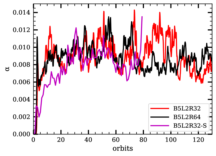
Figure 1.— The evolution of the $\alpha$-parameter. $\alpha$ increases initially and reaches the steady state after about 10 orbits for the unstratified simulations (B5L2R32 and B5L2R64) and after about 30 orbits for the stratified simulation (B5L2R32-S). The unstratified simulation B5L2R32 and stratified simulation B5L2R32-S give very similar values of $\alpha$ in steady states (see also Table 4). $\alpha$ is already converged with a numerical resolution of 32 cells per $L_{0}$ (B5L2R32), although the kinetic energy spectrum is not converged until a much higher resolution is used (see Figure 2 and discussions). Similar behaviors of $\alpha$ are found in all other simulations that are not plotted here.

Table 4Global properties of the MRI simulations in steady states

Model	$\sqrt{\langle\delta v^{2}\rangle}/c_{s}$	$\sqrt{\langle v_{A,z}^{2}\rangle}/c_{s}$	$\sqrt{\langle B_{z}^{2}\rangle}/B_{\mathrm{init}}$	$\alpha_{R}/10^{-3}$	$\alpha_{\mathrm{Maxw}}/10^{-3}$	$\alpha/10^{-3}$	$Q_{z}$
B5L2R32	$0.14\pm 0.02$	$0.20\pm 0.02$	$8.63\pm 1.33$	$1.68\pm 0.46$	$7.06\pm 1.61$	$8.74\pm 2.02$	$8$
B5L2R64	$0.13\pm 0.01$	$0.20\pm 0.01$	$9.50\pm 0.62$	$1.49\pm 0.19$	$6.85\pm 0.78$	$8.35\pm 0.94$	$17$
B5L2R128	$0.14\pm 0.01$	$0.22\pm 0.02$	$11.5\pm 0.7$	$1.49\pm 0.18$	$7.89\pm 0.82$	$9.38\pm 0.95$	$41$
B5L1R128	$0.10\pm 0.01$	$0.16\pm 0.02$	$9.52\pm 1.00$	$0.83\pm 0.18$	$4.28\pm 0.79$	$5.12\pm 0.93$	$34$
B5L1R256	$0.14\pm 0.01$	$0.23\pm 0.03$	$15.1\pm 1.6$	$1.29\pm 0.36$	$8.03\pm 1.39$	$9.32\pm 1.66$	$109$
B5L4R64	$0.15\pm 0.01$	$0.22\pm 0.01$	$10.4\pm 0.6$	$2.02\pm 0.25$	$8.20\pm 0.86$	$10.2\pm 1.0$	$19$
B4L2R64	$0.24\pm 0.02$	$0.40\pm 0.05$	$7.71\pm 0.82$	$4.78\pm 1.09$	$23.6\pm 3.6$	$28.4\pm 4.3$	$44$
B4L2R64-O3	$0.30\pm 0.03$	$0.46\pm 0.04$	$7.53\pm 0.86$	$9.04\pm 1.46$	$33.6\pm 5.3$	$42.6\pm 6.7$	$14$
B5L2R32-S	$0.15\pm 0.01$	$0.26\pm 0.09$	$8.69\pm 0.82$	$1.69\pm 0.28$	$6.93\pm 1.10$	$8.62\pm 1.30$	$8$

4.1.2 Driven Turbulence Simulations

As the energy is injected into the simulation domain, the kinetic (and magnetic, for MHD simulations) energy increases initially, and reaches a steady state after $t\gtrsim 40t_{0}$, about 4 times the turbulent crossing time. We run the simulations until $90t_{0}$, and analyse the results using the outputs in the steady state during $50-90t_{0}$.

The global properties of the simulations in steady states are summarized in Table 5. The average turbulent velocity, $\sqrt{\langle\delta v^{2}\rangle}/c_{s}\approx 0.10-0.15$, is similar to that in the MRI simulations (Table 5). In the MHD simulations, the magnetic energy is similar to the kinetic energy in the isotropic driving case (DR200B5), but is only a small fraction of the kinetic energy in the compressive driving case (DR200B5C). For the HD simulations, the total kinetic energy is converged with a resolution of 200 grid cells per $L_{0}$, for both the isotropic and compressive driving. Due to the constraints on computational resources, the MHD simulations are only performed at a resolution of 200 grid cells per $L_{0}$.

Table 5Global properties of the driven turbulence simulations in steady states

Model ID	$\sqrt{\langle\delta v^{2}\rangle}/c_{s}$	$\sqrt{\langle v_{A,z}^{2}\rangle}/c_{s}$
DR200	$0.14\pm 0.003$	-
DR400	$0.15\pm 0.002$	-
DR200C	$0.10\pm 0.01$	-
DR400C	$0.10\pm 0.01$	-
DR200B5	$0.10\pm 0.004$	$0.08\pm 0.005$
DR200B5C	$0.10\pm 0.01$	$0.0051\pm 0.0001$

4.2. Kinetic Energy Spectrum

The turbulence energy spectra of the MRI simulations are shown in Figure 2 left panel. The solenoidal modes dominate, containing more than 95% of the total turbulent kinetic energy. This is not surprising, since the linear analysis of the MRI already indicates that the instability can arise in incompressible fluid (Balbus & Hawley 1991). The turbulence energy spectra $E(k)$ drops steeply at $k/(2\pi)\gtrsim 0.1/\Delta x$ due to numerical dissipation, as no explicit dissipation is included. $E(k)$ shows a power-law dependence on $k$ over the middle range of $k$. Simulations with lower resolutions $L_{0}/\Delta x\leq 64$, such as B5L2R64, suffers from insufficient dynamical range, and do not show a converged power-law slope due to numerical dissipation. For higher resolution simulations showing a converged power-law slope, we fit simulations B5L2R128 and B5L1R128 over $4<k/(2\pi)<10$ and simulation B5L1R256 over $4<k/(2\pi)<20$ with a power-law function $E(k)\propto k^{-p}$ using the least square method, which yields an average of $p=1.32$. We estimate an error of $0.02$ for $p$, based on the error of fitting and the variation of $p$ when changing the range of $k$ for fitting. This slope is consistent with $k^{-4/3}$, and is shallower than predictions from both the Kolmogorov ($k^{-5/3}$) and the IK ($k^{-3/2}$) theories.

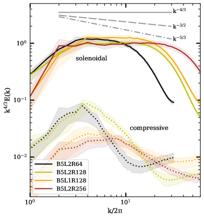
(a) MRI turbulence

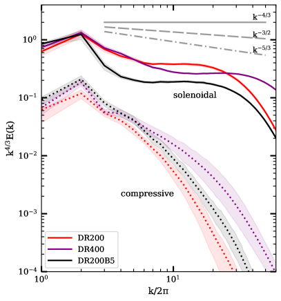
(b) isotropically driven turbulence

Figure 2.— The kinetic energy spectrum in the MRI (left panel) and isotropically driven (right panel) turbulence simulations. The $y$-axis is compensated by $k^{4/3}$, and normalized with the total turbulent kinetic energy $\int\mathrm{d}kE(k)$ for each model. The time-averaged spectra in different simulation models are decomposed into solenoidal and compressive modes, shown with the solid and dashed lines (see figure legend). The shaded area indicates the $1$-$\sigma$ dispersion among the different time snapshots. The gray solid, dash, and dash-dotted lines show the power laws for $k^{-4/3}$, IK ($k^{-3/2}$), and Kolmogorov ($k^{-5/3}$) energy spectra. The total energy spectra in both the MRI and isotropically driven turbulence are dominated by the solenoidal modes, and show a power-law range near the dissipation scale. Fitting of the turbulence energy spectra in the three high resolutions MRI simulations (B5L2R128, B5L1R128, B5L2R256) gives a slope of $E(k)\propto k^{-1.32\pm 0.02}$ in the power-law ranges, consistent with the $k^{-4/3}$ energy spectrum.

In order to understand the $k^{-4/3}$ slope, we plot the energy spectrum from driven turbulence simulations in Figure 2 right panel. With the isotropic driving, the energy spectrum shows a slope consistent with $k^{-4/3}$ in both the HD and MHD simulations. The slope is converged with a resolution $L_{0}/\Delta x\geq 200$ in the HD simulations. This implies that the $k^{-4/3}$ slope is an intrinsic property of the turbulence even in the hydrodynamic case, and not a phenomenon that is only caused by magnetic fields. With compressive driving, on the other hand, the energy spectrum shows a steeper slope close to $k^{-7/3}$. This steepening of the energy spectrum in compressive driving turbulence is also observed in numerical simulations with a much higher resolution by Grete et al. (2018).

There have been a great deal of work on the MHD turbulence driven by different mechanisms and with various numerical techniques. The findings in the literature is summarized in Table 6. In all of the cases, $p$ smaller than $5/3$ is observed, while a slope similar to $p=4/3$ is reported in many studies with different turbulence driving mechanisms, equations of state, magnetic field strengths, and numerical codes.

The shallower energy spectrum near the dissipation scale has long been observed by the fluid dynamics community in both numerical simulations and physical experiment, albeit it is less known to the astrophysics community (e.g. reviews by Sreenivasan 1995; Alexakis & Biferale 2018). This is often referred to as the “bottleneck” effect, and is suggested to be caused by the helicity cascade (Kurien et al. 2004): the $k^{-4/3}$ slope can arise when the helicity cascade timescale dominates over the energy cascade timescale, and the bottleneck region is less pronounced when the turbulence driving contains less helicity. Recent high resolution simulations of hydrodynamic turbulence by Ishihara et al. (2016) shows that the bottleneck region and a subsequent “tilt” extends over 2 – 3 dex near the dissipation scale, before the Kolmogorov spectrum is observed on larger scales.

This cautions that a power-law region with converged slope, as is observed in our simulations, does not mean that it is the inertial range. In the future, simulations with at least an order of magnitude higher resolution are needed to explore the inertial range of the MRI turbulence. This poses a significant challenge on computational resources: the computation time step scales as $N^{4}$ ($N^{3}$ from the spacial resolution in three dimensions, and $N$ from the reduced time step) in grid-based codes, where $N$ is the number of resolution elements per dimension. The spectral method is widely used for driven turbulence simulations, but requires complex treatment to handle the background shear and boundary conditions in shearing box simulations. Lesur & Longaretti (2011) and Walker et al. (2016) used the spectral code Snoopy to simulate MRI turbulence, and obtained a highest resolution per $H$ about twice of that in this work.

Table 6Kinetic and magnetic power spectra in MHD turbulence reported in the literature

Ref.	Turbulence Generation	$\beta_{\mathrm{init}}$	Driven?	EOS	Codes	$N$	$p$	$p_{M}$
1	Kelvin-Helmholtz instability	$5000$	No	adiabatic	Athena	512	$1.33\pm 0.02$	$1.62\pm 0.02$
2	shear-Alfven waves at large scales	$0.33$	No	isothermal	PLUTO, VPIC	1152	$\sim 1.3$	$\sim 1.3$
3	kinetic energy injection at large scales	$0.02$	Yes	adiabatic	Athena	1024	$1.38$	$1.22$
4	external force at large scales	$5$, $72$	Yes	isothermal	Enzo, Athena	1024	$\sim 4/3$	$\sim 1.7$
5	MRI with viscosity and resistivity	$400$	MRI	isothermal	ZEUS	512	$\sim 1.5$	$\sim 0$
6	MRI with viscosity and resistivity	$1000$	MRI	incompressible	Snoopy	192	$\sim 1.5$	-
7	MRI with viscosity and resistivity	$1100$	MRI	incompressible	Snoopy	512	$\sim 1.5$	$\sim 2$

Another important parameter for the kinetic energy spectrum is the injection scale. OC2007 assume that the injection scale $k_{L}$ is the disk scale-height $H$, and $E(k)=0$ for $k<k_{L}$. In reality, $E(k)$ never drops to zero in MRI turbulence, as shown in Figure 2. Therefore, one can define the effective injection scale as the peak of $kE(k)$ in Figure 3, the scale where most of the kinetic energy is concentrated at. We found that the injection scale in MRI turbulence can be approximated by an estimation of the fastest growing mode of the linear MRI (Balbus & Hawley 1991),

$$k_{\mathrm{MRI}}=\sqrt{\frac{15}{16}}\frac{\Omega}{\langle v_{A,z}\rangle}.$$ (16)

$k_{\mathrm{MRI}}$ for simulations with different initial magnetic field strengths and orbital frequencies are shown as the vertical dashed lines in the left panel of Figure 3. In the right panel of Figure 3, we show ath the injection scale in the driven turbulence simulations is, indeed, close to the peak of $kE(k)$. We note that contrary to the assumption in OC2007 that the injection scale is at the disk scale height $H$, $k_{\mathrm{MRI}}$ is determined by the magnetic field strength instead of $H$. For a weak vertical magnetic field in our simulations, $\langle v_{A,z}\rangle$ is smaller than the sound speed, and the length scale $1/k_{\mathrm{MRI}}$ is smaller than $H$.

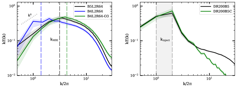
Figure 3.— Kinetic energy spectra compensated by $k$, for MRI (left panel) and driven turbulence (right panel) simulations. The $y$-axis is normalized with the total turbulent kinetic energy $\int\mathrm{d}kE(k)$ for each model. The solid lines show the time-averaged energy spectrum in different simulation models (see figure legend), and the shaded area indicates the $1$-$\sigma$ dispersion among different time snapshots. The vertical dashed lines in the left panel denote the estimation for the fastest growing mode for the MRI, $k_{\mathrm{MRI}}$ (Equation (16)). In the right panel, the vertical dashed lines bounding the shaded area indicate the range of scales where kinetic energy is injected to drive the turbulence. The peak of $kE(k)$, representing the maximum kinetic energy density, matches the expected energy injection scale of $k_{\mathrm{MRI}}$ and $k_{\mathrm{inject}}$.

4.3. Magnetic Energy Spectrum

Unlike the kinetic energy spectrum, the magnetic energy spectrum does not show any power-law behavior (Figure 4). $E_{M}(k)$ is roughly constant across a wide range of $k$, until it drops off quickly at larger $k$ due to numerical dissipation. In MRI turbulence, the magnetic energy $kE_{M}(k)$ peaks near the dissipation scale (Figure 4, left panel), possibly due to the injection of magnetic energy at small scales by the dynamo mechanism proposed by Schekochihin et al. (2002). Similar results also have been found in MRI simulations by Fromang (2010) with explicit resistivity and viscosity. There is also evidence that the position of the peak may depend on the magnetic Prandtl number, and not always be at the resistive scale (Subramanian 1999; Haugen et al. 2003). In ideal MHD simulations, it is difficult to quantify the effective Prandtl number from numerical dissipation, and therefore future simulations with explicit dissipation are needed to address this issue.

In driven turbulence simulations, $kE_{M}(k)$ peaks at large scales, where perturbations are driven (Figure 4 right panel), consistent with injection of magnetic energy by the perturbation. Figure 5 illustrates the magnetic field lines, which shows visually that small-scale perturbations of the magnetic field are more prominent in the MRI turbulence than in the driven turbulence.

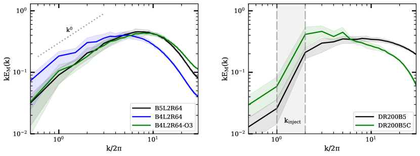
Figure 4.— The magnetic energy spectrum $E_{M}(k)$ compensated by $k$, for MRI (left panel) and driven turbulence (right panel) simulations, similar to the kinetic energy spectrum in Figure 3. The peak of the magnetic energy $kE_{M}(k)$ is located near the dissipation scale for MRI simulations (left panel), and near the injection scale for driven turbulence simulations (right panel). The dotted line in the left panel shows that $E_{M}(k)$ in the MRI turbulence is close to a constant in a wide range of $k$ before the numerical dissipation becomes important.

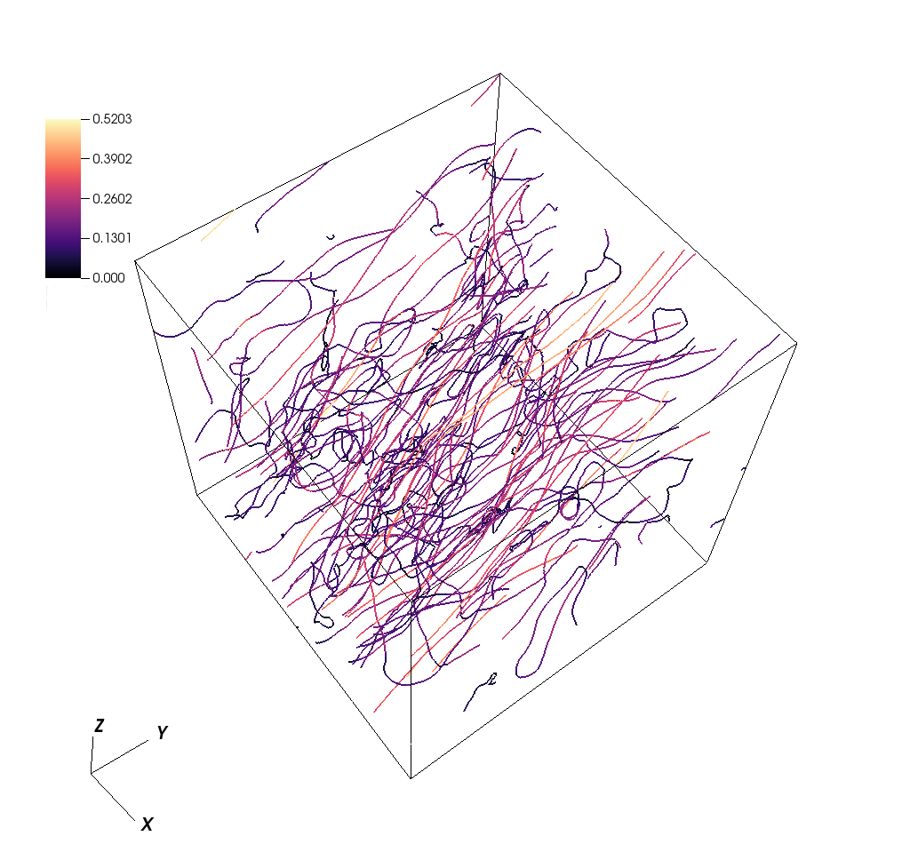
(a) MRI

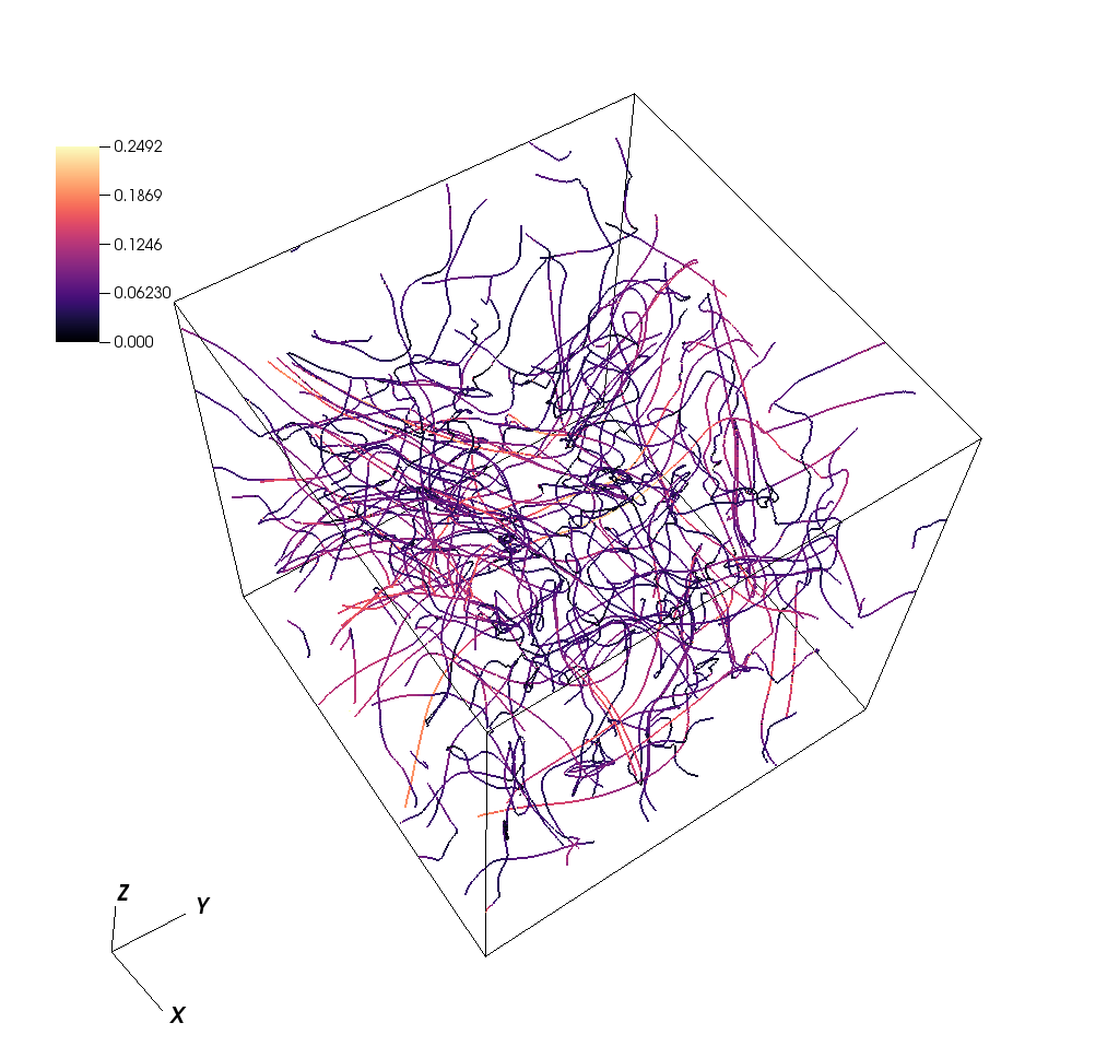
(b) driven turbulence

Figure 5.— Visualization of the magnetic field lines in (a) MRI simulation B5L1R256 and (b) driven turbulence simulation DR200B5. The snapshots are taken at $t=90t_{0}$, when both simulations already reached steady state. The simulation box-size is $L_{0}$ on all sides. The color of the streamline shows the magnetic field strength (stronger field in lighter colors, see legends). Compared to the driven turbulence, the magnetic field in the MRI turbulence has more power on the small scales (Figure 4), and a mean field along y-axis due to the shearing motion.

4.4. The Effect of Stratification

In order to investigate the effect of stratification on the turbulence, we carry out stratified simulation B5L2R32_S, with the initial conditions in the mid-plane similar to those the unstratified simulation B5L2R32. Due to the larger box and fast outflow at the $z$-boundary, the stratified simulation is much more computationally costly, and thus the resolution is limited. However, this still allows us to compare the positions of the peaks of the energy spectra in the stratified and unstratified models.

Figure 6 shows the kinetic and magnetic energy spectra in the stratified simulation B5L2R32_S and unstratified simulation B5L2R32. The higher-resolution unstratified simulation B5L2R64 is also plotted for reference. Both the kinetic and magnetic energy spectra are similar between B5L2R32_S in the midplane and the unstratified simulation B5L2R32, justifying the use of the unstratified simulations for the mid-plane conditions. The maximum of the kinetic energy density is similar to $k_{\mathrm{MRI}}$ in both the disk mid-plane and corona, although the gas density drops by nearly an order of magnitude from the disk mid-plane to the corona region. The magnetic energy spectrum in the corona region, however, differs significantly from the disk mid-plane, and peaks instead at the largest scales. This is similar to the findings by Nauman & Blackman (2014) and Blackman & Nauman (2015), who pointed out the potential importance of non-local transport in the disk. Thorough investigations of the impact of stratification and global geometry on the shape of the energy spectrum, however, require global disk simulations with very high resolution, which is beyond the scope of this paper.

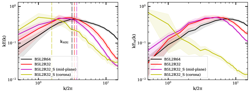
Figure 6.— Kinetic (left panel) and magnetic (right panel) energy spectra compensated by $k$, for stratified and unstratified simulations (see legend), similar to the left panels in Figures 3 and 4. The energy spectra are shown in the mid-plane ($-1<z<1$) and upper corona ($1<z<3$, the spectra for $-3<z<-1$ are very similar) for the stratified simulation B5L2R32_S. The shapes of the spectra are similar between the stratified simulation B5L2R32_S in the mid-plane region, and the unstratified simulation B5L2R32. The fastest growing mode for the MRI, $k_{\mathrm{MRI}}$ (Equation (16)), reasonably matches the maximum of the kinetic energy density in both the mid-plane and the corona regions. The magnetic energy spectrum in the corona region, however, is distinctively different from that in the disk mid-plane, and peaks at much larger scales.

4.5. Auto-correlation Time

The auto-correlation of turbulence eddies as a function of time can be well fitted by Equation (5) in the power-law range of the kinetic energy spectrum (Figures 2), where the influence from energy injection at large scales and numerical dissipation at small scales is small. Figure 7 shows a summary of $\tau(k)$ obtained from the simulations. $\tau(k)$ in the MRI turbulence is roughly a constant at large scales, limited by the shearing timescale $\tau_{\mathrm{shear}}=1/\Omega$, and shows a power-law drop off at small scales, limited by the eddy crossing time $\tau_{\mathrm{cross}}=1/(k\delta v(k))=1/(k\sqrt{2kE(k)})$. The power-law slope is converged for the MRI simulation B5L2H64 and B5L2H128, as well as the driven turbulence simulation DR200 and DR400. Fitting with $\tau(k)\propto k^{-m}$ in the power-law range gives a slope of $m=1.11\pm 0.07$ for the MRI simulation B5L2H64 and B5L2H128 between $3<k/(2\pi)<9$, and $m=1.16\pm 0.02$ for the driven turbulence simulation DR200 and DR400 between $9<k/(2\pi)<20$. This is somewhat steeper than the slope of $\tau(k)\propto k^{-2/3}$ predicted from the eddy crossing time for a Kolmogorov spectrum and of $\tau(k)\propto k^{-5/6}$ for a $E(k)\propto k^{4/3}$ spectrum (as found in Section 4.3).

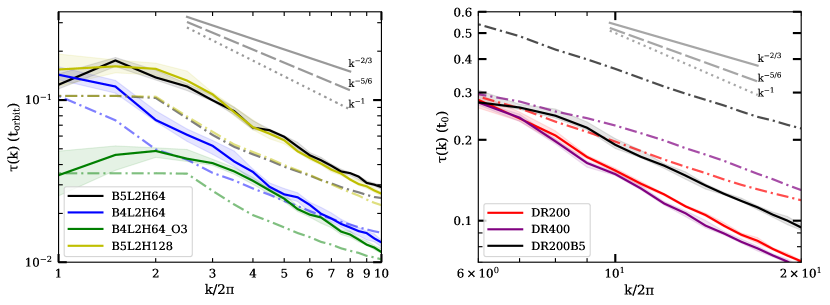
Figure 7.— The eddy auto-correlation time obtained from the MRI (left panel) and driven turbulence (right panel) simulations. The solid lines show the time-averaged $\tau(k)$ in different simulation models (see figure legend), and the shaded area indicates the $1$-$\sigma$ dispersion among different time snapshots. The dashed-dotted lines of the corresponding color shows the expected $\tau(k)$ in each model: the minimum of the shearing timescale and the eddy crossing time in the MRI simulations (left panel), and the eddy crossing time only in the driven turbulence simulations (right panel). The gray solid, dashed and dotted lines indicate a power-law slope of $k^{-2/3}$ (Kolmogorov eddy crossing time), $k^{-5/6}$ (eddy crossing time for $k^{-4/3}$ energy spectrum ), and $k^{-1}$.

5. Conclusions

In this paper, we investigate the key underlying assumptions for the turbulence properties governing the grain growth in protoplanetary disks. We carry out ideal MHD shearing-box simulations to investigate the MRI turbulence in protoplanetary disks. We also perform HD and MHD driven turbulence simulations to compare with the MRI turbulence.

Both the energy spectrum $E(k)$ and the auto-correlation time $\tau(k)$ of the MRI turbulence in our simulations deviate from those in the Kolmogorov turbulence, which is widely adopted by the current grain collisional velocity calculations such as OC2007. The main findings of this paper are summarized as follows:

1. The MRI turbulence is largely solenoidal. We observe $E(k)\propto k^{-4/3}$ in the MRI turbulence, as well as in an isotropically driven turbulence with and without magnetic field, over more than 1 dex near the dissipation scale (Figures 2). This power-law slope appears to be converged in terms of numerical resolution, and to be due to the bottleneck effect.

2. The kinetic turbulence energy spectrum $E(k)$ converges at a much higher resolution ($128$ cells per $H$) than the turbulence $\alpha$-parameter ($32$ cells per $H$).

3. The kinetic energy in the MRI turbulence peaks at the fastest growing mode of the MRI (Figure 3), which does not necessarily match the disk scale height as assumed by OC2007. In contrast, the magnetic energy peaks at the dissipation scale (Figure 4).

4. The magnetic energy spectrum $E_{M}(k)$ in the MRI turbulence does not show a clear power-law range, and is almost constant over approximately 1 dex near the dissipation scale (Figure 4).

5. The turbulence autocorrelation time $\tau(k)$ in the MRI turbulence is nearly constant at large scales, limited by the shearing timescale, and shows a power-law drop close to $k^{-1}$ at small scales, with a slope slightly steeper than the eddy crossing time (Figure 7).

Due to the bottleneck effect near the dissipation scale, the power-law slopes of $E(k)$ and $\tau(k)$ observed in our simulations may not represent those in the inertial range of the turbulence. Still, only slight changes in the shapes of $E(k)$ and $\tau(k)$ can have a significant effect on the grain collisional velocities. In a future paper, we plan to investigate the potential impact of the turbulence properties on the grain size evolution in protoplanetary disks.

6. Acknowledgement

We thank the anonymous referee for a constructive review, which helped to improve the quality and clarity of this paper. M. Gong thanks Xuening Bai and Jake Simon for their generous help and advices on the use of the Athena code and related scientific discussions, Geoffroy Lesur for his helpful suggestions on turbulence analysis, and Chang-Goo Kim for his implementation of the turbulence driving module in the Athena++ code.

Appendix A Calculation of Turbulence Properties from Numerical Simulations

The turbulence power spectrum $P(k)$ and auto-correlation time $\tau(k)$ determine the collisional velocities between dust grains. In OC2007, $P(k)$ and $\tau(k)$ are assumed to follow the analytic expression of Kolmogorov turbulence: $E(k)\equiv 4\pi k^{2}P(k)\propto k^{-5/3}$ and $\tau(k)=1/(k\sqrt{2kE(k)})$. To study the MRI turbulence in protoplanetary disks, we derive $P(k)$ and $\tau(k)$ from numerical simulations, using the procedures described below.

As the simulations are preformed on a discrete grid, we use the discrete fast Fourier transform to calculate $\widetilde{y}(\mathbf{k})$ for the physical variables $y(\mathbf{x})$ in our simulations. The resolution of $\widetilde{y}(\mathbf{k})$ in $\mathbf{k}$ space is $\mathrm{d}k_{i}=2\pi/L_{i},~{}i=x,y,z$. $\widetilde{y}(k)$ is then calculated by averaging over co-centric shells of width $\mathrm{d}k=\mathrm{max}\{\mathrm{d}k_{x},\mathrm{d}k_{y},\mathrm{d}k_{z}\}$ around the origin in $\mathbf{k}$ space . The kinetic power spectrum $P(k)$ is then obtained from Equation (1). To reduce noise, we average $P(k)$ over a period of time when the simulations already reach quasi-equilibrium (see Section 4.1). We produce outputs of the simulations at intervals of $t_{\mathrm{orbit}}$, and the average $P(k)$ is calculated from the outputs during simulation time $40t_{\mathrm{orbit}}-80t_{\mathrm{orbit}}$ for model B5L2R32-s and $90t_{\mathrm{orbit}}-130t_{\mathrm{orbit}}$ for all other models.

$\tau(k)$ is obtained by fitting Equation (5), where the values of $f(\Delta t)$ are calculated directly from the numerical simulations, and $|\widetilde{\delta\mathbf{v}}(\mathbf{k},t_{s})|^{2}$ and $\tau(k)$ are treated as constant parameters obtained from the least-square fitting of $f(\Delta t)$ as a function of $\Delta t$. We output simulations and calculate $f(\Delta t)$ at small time intervals $\mathrm{d}t_{\mathrm{out}}\ll\tau(k)$, to obtain enough time resolution in $\Delta t$ to accurately fit $\tau(k)$. We also sample a range of $t_{s}$ to characterize the noise in $\tau(k)$. We transfer the turbulent velocity field $\delta\mathbf{v}$ onto the shearing frame $y^{\prime}=y+q\Omega x\Delta t$, so $\tau(k)$ is only determined by the turbulent motions.

References

- Alexakis & Biferale (2018) Alexakis, A., & Biferale, L. 2018, Phys. Rep., 767, 1
- Bai (2017) Bai, X.-N. 2017, ApJ, 845, 75
- Bai & Stone (2013) Bai, X.-N., & Stone, J. M. 2013, ApJ, 767, 30
- Balbus & Hawley (1991) Balbus, S. A., & Hawley, J. F. 1991, ApJ, 376, 214
- Birnstiel et al. (2010) Birnstiel, T., Dullemond, C. P., & Brauer, F. 2010, A&A, 513, A79
- Birnstiel et al. (2016) Birnstiel, T., Fang, M., & Johansen, A. 2016, Space Sci. Rev., 205, 41
- Birnstiel et al. (2011) Birnstiel, T., Ormel, C. W., & Dullemond, C. P. 2011, A&A, 525, A11
- Blackman & Nauman (2015) Blackman, E. G., & Nauman, F. 2015, Journal of Plasma Physics, 81, 395810505
- Blum & Wurm (2008) Blum, J., & Wurm, G. 2008, ARA&A, 46, 21
- Brauer et al. (2008) Brauer, F., Dullemond, C. P., & Henning, T. 2008, A&A, 480, 859
- Epstein (1924) Epstein, P. S. 1924, Phys. Rev., 23, 710
- Flaherty et al. (2015) Flaherty, K. M., Hughes, A. M., Rosenfeld, K. A., et al. 2015, ApJ, 813, 99
- Flaherty et al. (2018) Flaherty, K. M., Hughes, A. M., Teague, R., et al. 2018, ApJ, 856, 117
- Fromang (2010) Fromang, S. 2010, A&A, 514, L5
- Garaud et al. (2013) Garaud, P., Meru, F., Galvagni, M., & Olczak, C. 2013, ApJ, 764, 146
- Grete et al. (2018) Grete, P., O’Shea, B. W., & Beckwith, K. 2018, ApJ, 858, L19
- Grete et al. (2017) Grete, P., O’Shea, B. W., Beckwith, K., Schmidt, W., & Christlieb, A. 2017, Physics of Plasmas, 24, 092311
- Haugen et al. (2003) Haugen, N. E. L., Brandenburg, A., & Dobler, W. 2003, ApJ, 597, L141
- Hawley et al. (1995) Hawley, J. F., Gammie, C. F., & Balbus, S. A. 1995, ApJ, 440, 742
- Hawley et al. (2011) Hawley, J. F., Guan, X., & Krolik, J. H. 2011, ApJ, 738, 84
- Hayashi (1981) Hayashi, C. 1981, Progress of Theoretical Physics Supplement, 70, 35
- Iroshnikov (1964) Iroshnikov, P. S. 1964, Soviet Ast., 7, 566
- Ishihara et al. (2016) Ishihara, T., Morishita, K., Yokokawa, M., Uno, A., & Kaneda, Y. 2016, Phys. Rev. Fluids, 1, 082403
- Johnson et al. (2008) Johnson, B. M., Guan, X., & Gammie, C. F. 2008, The Astrophysical Journal Supplement Series, 177, 373
- Kraichnan (1965) Kraichnan, R. H. 1965, Physics of Fluids, 8, 1385
- Kurien et al. (2004) Kurien, S., Taylor, M. A., & Matsumoto, T. 2004, Phys. Rev. E, 69, 066313
- Lemaster & Stone (2009) Lemaster, M. N., & Stone, J. M. 2009, ApJ, 691, 1092
- Lesur & Longaretti (2011) Lesur, G., & Longaretti, P. Y. 2011, A&A, 528, A17
- Makwana et al. (2015) Makwana, K. D., Zhdankin, V., Li, H., Daughton, W., & Cattaneo, F. 2015, Physics of Plasmas, 22, 042902
- Markiewicz et al. (1991) Markiewicz, W. J., Mizuno, H., & Voelk, H. J. 1991, A&A, 242, 286
- Masset (2000) Masset, F. 2000, Astronomy and Astrophysics Supplement Series, 141, 165
- Miyoshi & Kusano (2005) Miyoshi, T., & Kusano, K. 2005, Journal of Computational Physics, 208, 315
- Nauman & Blackman (2014) Nauman, F., & Blackman, E. G. 2014, MNRAS, 441, 1855
- Ormel & Cuzzi (2007) Ormel, C. W., & Cuzzi, J. N. 2007, A&A, 466, 413
- Pinte et al. (2016) Pinte, C., Dent, W. R. F., Ménard, F., et al. 2016, ApJ, 816, 25
- Salvesen et al. (2014) Salvesen, G., Beckwith, K., Simon, J. B., O’Neill, S. M., & Begelman, M. C. 2014, MNRAS, 438, 1355
- Sano et al. (2004) Sano, T., Inutsuka, S.-i., Turner, N. J., & Stone, J. M. 2004, ApJ, 605, 321
- Schekochihin et al. (2002) Schekochihin, A. A., Maron, J. L., Cowley, S. C., & McWilliams, J. C. 2002, ApJ, 576, 806
- Schmidt et al. (2009) Schmidt, W., Federrath, C., Hupp, M., Kern, S., & Niemeyer, J. C. 2009, A&A, 494, 127
- Shi et al. (2016) Shi, J.-M., Stone, J. M., & Huang, C. X. 2016, MNRAS, 456, 2273
- Simon et al. (2018) Simon, J. B., Bai, X.-N., Flaherty, K. M., & Hughes, A. M. 2018, ApJ, 865, 10
- Simon et al. (2012) Simon, J. B., Beckwith, K., & Armitage, P. J. 2012, MNRAS, 422, 2685
- Sreenivasan (1995) Sreenivasan, K. R. 1995, Physics of Fluids, 7, 2778
- Stone & Gardiner (2009) Stone, J. M., & Gardiner, T. 2009, New A, 14, 139
- Stone & Gardiner (2010) Stone, J. M., & Gardiner, T. A. 2010, ApJS, 189, 142
- Stone et al. (2008) Stone, J. M., Gardiner, T. A., Teuben, P., Hawley, J. F., & Simon, J. B. 2008, ApJS, 178, 137
- Stone et al. (1996) Stone, J. M., Hawley, J. F., Gammie, C. F., & Balbus, S. A. 1996, ApJ, 463, 656
- Stone et al. (2019) Stone, J. M., Tomida, K., White, C. J., & Felker, K. G. 2019, submitted to American Astronomical Society journals
- Subramanian (1999) Subramanian, K. 1999, Phys. Rev. Lett., 83, 2957
- Teague et al. (2016) Teague, R., Guilloteau, S., Semenov, D., et al. 2016, A&A, 592, A49
- Testi et al. (2014) Testi, L., Birnstiel, T., Ricci, L., et al. 2014, in Protostars and Planets VI, ed. H. Beuther, R. S. Klessen, C. P. Dullemond, & T. Henning, 339
- Völk et al. (1980) Völk, H. J., Jones, F. C., Morfill, G. E., & Roeser, S. 1980, A&A, 85, 316
- Walker et al. (2016) Walker, J., Lesur, G., & Boldyrev, S. 2016, MNRAS, 457, L39
- White et al. (2016) White, C. J., Stone, J. M., & Gammie, C. F. 2016, ApJS, 225, 22
- Zhu & Stone (2014) Zhu, Z., & Stone, J. M. 2014, ApJ, 795, 53