Precise determination of proton magnetic radius from electron scattering data

Abstract

We extract the proton magnetic radius from the high-precision electron-proton elastic scattering cross section data. Our theoretical framework combines dispersion analysis and chiral effective field theory and implements the dynamics governing the shape of the low-$Q^{2}$ form factors. It allows us to use data up to $Q^{2}\sim$ 0.5 GeV² for constraining the radii and overcomes the difficulties of empirical fits and $Q^{2}\rightarrow 0$ extrapolation. We obtain a magnetic radius $r_{M}^{p}$ = 0.850 $\pm$0.001 (fit 68%) $\pm$0.010 (theory full range) fm, significantly different from earlier results obtained from the same data, and close to the extracted electric radius $r_{E}^{p}$ = 0.842 $\pm$0.002 (fit) $\pm$0.010 (theory) fm.

I Introduction

The electromagnetic form factors (EM FFs) are the most basic expressions of the nucleon’s finite spatial extent and composite internal structure. They describe the elastic response to external electric and magnetic fields as a function of the 4-momentum transfer $Q^{2}$ and can be associated with the spatial distributions of charge and current in nucleon. The traditional representation of FFs in terms of 3-dimensional spatial densities at fixed instant time $x^{0}=$ const. is appropriate only for nonrelativistic systems such as nuclei Miller (2019). For relativistic systems such as hadrons, the spatial structure is expressed through 2-dimensional transverse densities at fixed light-front time $x^{+}=x^{0}+x^{3}=$ const. In the context of QCD these transverse densities can be regarded as projections of the nucleon’s partonic structure (generalized parton distributions) Diehl (2003); Belitsky and Radyushkin (2005); Boffi and Pasquini (2007). The EM FFs thus reveal aspects of the spatial distribution of quarks and their orbital motion and spin and have become objects of great interest in nucleon structure studies Punjabi et al. (2015); Pacetti et al. (2015).

The value of the electric and magnetic proton FFs at $Q^{2}=0$ is given by the total charge and magnetic moment of the proton, $G_{E}^{p}(0)=1,G_{M}^{p}(0)=\mu^{p}=2.793$. The leading information about the spatial structure is in the first derivatives of the FFs at $Q^{2}=0$. They are conventionally expressed in terms of the equivalent electric and magnetic 3-dimensional root-mean-square radii,

$$\frac{dG_{E}^{p}}{dQ^{2}}(0)\;=\;-\frac{(r_{E}^{p})^{2}}{6},\hskip 20.00003pt\frac{1}{\mu^{p}}\frac{dG_{M}^{p}}{dQ^{2}}(0)\;=\;-\frac{(r_{M}^{p})^{2}}{6};$$ (1)

this does not imply an actual physical interpretation in terms of 3-dimensional densities; the proper interpretation in terms of 2-dimensional densities is discussed below Miller (2019). Besides their importance for nucleon structure, the FF derivatives are needed in tests of atomic bound-state calculations in quantum electrodynamics and in precision measurements of the Rydberg constant Eides et al. (2001); Pohl et al. (2010).

The proton electric (or charge) radius is extracted from the proton FFs measured in electron-proton elastic scattering, and from the nuclear corrections to atomic energy levels (electronic and muonic hydrogen) measured in precision spectroscopy experiments; see Refs. Pohl et al. (2013); Carlson (2015) for a review. Apparent discrepancies between the different extraction methods (“proton radius puzzle”) have engendered intense experimental and theoretical efforts, including dedicated new FF measurements at low $Q^{2}$ using electron and muon beams Xiong et al. (2019); Gilman et al. (2017). Recent results seem to converge around $r_{E}^{p}=0.84$ fm Higinbotham et al. (2016); Tietsinga et al. ; Xiong et al. (2019); Bezginov et al. (2019). The magnetic radius can be extracted only from elastic scattering measurements. Recent determinations based on the Mainz A1 data Bernauer et al. (2010, 2014), using methods developed in the context of the charge radius extraction, have resulted in a range of values that disagree with each other, $r_{M}^{p}=$ 0.78(2) fm Bernauer et al. (2010), 0.914(35)fm and 0.776(38)fm Lee et al. (2015), and significantly depart from older results $\sim$0.85 fm Belushkin et al. (2007). It is necessary to resolve these discrepancies and determine the proton magnetic radius with an overall accuracy and consistency commensurate with those achieved in the electric radius.

Here we report an extraction of the proton magnetic radius from electron scattering data using a novel theoretical framework based on dispersion analysis and chiral effective field theory (DI$\chi$EFT) Alarcón et al. (2019); Alarcón and Weiss (2017, 2018a, 2018b). It implements analyticity and the dynamics governing the shape of the low-$Q^{2}$ FFs and allows us to use data up to $Q^{2}\sim$ 0.5 GeV² for constraining the radii, increasing the sensitivity to the magnetic FF. It overcomes the difficulties in extraction methods based on empirical fits and $Q^{2}\rightarrow 0$ extrapolation (functional form bias, unstable extrapolation), particularly the issues related to the normalization of data sets taken at different incident energies. DI$\chi$EFT was used in Ref.Alarcón et al. (2019) to extract $r_{E}^{p}$ from an empirical FF parameterization Ye et al. (2018) and delivered a value of $r_{E}^{p}$ = 0.844(7) fm, as accepted in the CODATA 2018 update and confirmed by more recent measurements Tietsinga et al. ; Xiong et al. (2019); Bezginov et al. (2019). In this work we use the method to extract both $r_{M}^{p}$ and $r_{E}^{p}$ from a direct analysis of the cross section data, dominated by the Mainz A1 data Bernauer et al. (2010, 2014). We obtain $r_{M}^{p}$ = 0.850 $\pm$0.001 (fit 68%) $\pm$0.01 (theory full range) fm, significantly different from the values extracted from the same data using other methods Bernauer et al. (2010); Lee et al. (2015), and surprisingly close to $r_{E}^{p}$. In the course we also improve our extraction of $r_{E}^{p}$ and verify the robustness of the results.

II Method

DI$\chi$EFT is a method for calculating nucleon FFs combining dispersion analysis and chiral effective field theory. The theoretical foundations are described in detail in Refs. Alarcón and Weiss (2017, 2018a, 2018b); applications to FF fits are discussed in Ref. Alarcón et al. (2019). The FFs are represented as dispersion integrals over $t\equiv-Q^{2}$. The spectral functions on the two-pion cut at $t>4M_{\pi}^{2}$ are calculated using (i) the elastic unitarity relation; (ii) $\pi N$ amplitudes computed in $\chi$EFT at leading order, next-to-leading order, and partial next-to-next-to-leading order accuracy; (iii) the timelike pion FF measured in $e^{+}e^{-}$ annihilation experiments. The approach includes $\pi\pi$ rescattering effects and the $\rho$ resonance and generates accurate spectral functions up to $t\sim 1$ GeV². Higher-mass $t$-channel states are described by effective poles. The parameters specifying the dynamical input (the low-energy constants of the $\chi$EFT calculation, and the strength of the effective poles) are related by the sum rules of dispersion theory and can be expressed in terms of the nucleon charges, magnetic moments, and radii. For each (assumed) value of $r_{E}^{p}$ and $r_{M}^{p}$ the theory thus generates a unique prediction for $G_{E}^{p}(Q^{2})$ and $G_{M}^{p}(Q^{2})$ with controlled theoretical uncertainties; see Ref. Alarcón et al. (2019) for a summary plot. It predicts the “shape” of the spacelike FF as determined by analyticity (position of singularities) and dynamics (strength of singularities). In this way the values of the radii are correlated with the predicted behavior of the FFs at finite momentum transfers $Q^{2}\sim$ 1 GeV², allowing the use of such data for radius extraction. A computer code generating the DI$\chi$EFT FF predictions and further information are available .

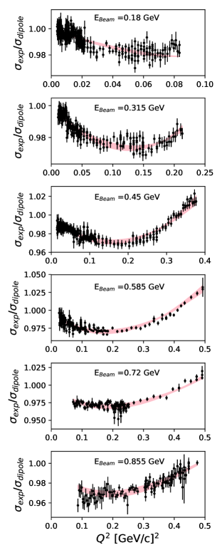
Figure 1: Data: Mainz A1 electron-proton elastic scattering cross section data Bernauer et al. (2010, 2014), with the normalization of sets determined by our fit. Band: Theoretical model (DI$\chi$EFT) with parameters $(r_{E}^{p},r_{M}^{p})$ obtained from our best fit. The band shows the range of the model predictions obtained by varying the parameters in the 68% confidence interval of the fit; it does not include the intrinsic theoretical uncertainty of the model Alarcón et al. (2019). Both data and model are divided by the cross section evaluated with the dipole FFs ($\Lambda^{2}=$ 0.71 GeV²).

For our radius extraction we use the high-precision data in electron-proton elastic scattering from the Mainz A1 experiment, which dominate the world data Bernauer et al. (2010, 2014). The experiment measured the elastic scattering cross section at momentum transfers $0.003\lesssim Q^{2}\lesssim 1$ GeV² and incident electron energies $E_{\rm Beam}$ from 0.18 to 0.855 GeV. The 2-dimensional data cover the cross section at a fixed $Q^{2}$ at various values of the virtual photon polarization parameter, $\epsilon$, and allow for separation of the contributions of $G_{E}^{p}(Q^{2})$ and $G_{M}^{p}(Q^{2})$ through global fits, generalizing the traditional Rosenbluth method Bernauer et al. (2010, 2014).

An important issue in global fits is the normalization of the data sets taken at different energies. The normalization of the cross section data (both absolute and relative, between different energies) is limited by the knowledge of the absolute luminosity in the different settings and subject to considerable uncertainties. The combination of data taken at different energies therefore requires rescaling of the data sets, which depends on the functional form of the FFs or on other assumptions. In the context of empirical fits the effect of the rescaling on the random uncertainties of the data was studied in detail in Refs. Bernauer et al. (2014); Lee et al. (2015). In the context of our approach this problem is naturally solved by the fact that the theoretical model predicts the shape of the FFs at finite $Q^{2}$ (in dependence of the radii). We can therefore perform a global fit with floating normalizations of the data sets, which can adjust themselves to the theoretical model; the physical information is in the variation of the data with $Q^{2}$, which tests the theoretical predictions for the shape and fixes the radius parameters through the best fit.

As the figure-of-merit for the global fit with floating normalizations we use a $\chi^{2}$ function of the form

$$\chi^{2} \equiv \chi^{2}(r_{E}^{p},r_{M}^{p};\Lambda_{1},...,\Lambda_{N_{\rm set}})$$ (2)

$$\equiv {N_{\rm dat}^{-1}}\sum_{\textrm{data $i$}}\left[\frac{\sigma_{{\rm thy},i}-\Lambda_{k(i)}\,\sigma_{{\rm exp},i}}{\Lambda_{k(i)}\,\Delta\sigma_{{\rm exp},i}}\right]^{2},$$

$$\sigma_{{\rm thy},i} \equiv \sigma(E_{i},Q^{2}_{i})[\textrm{DI$\chi$EFT, params $r_{E}^{p},r_{M}^{p}$}].$$ (3)

The summation is over the $N_{\rm dat}$ data points labeled by $i$. $\sigma_{{\rm thy},i}$ is the theoretical electron-proton elastic scattering cross section at the kinematic point $(E_{i},Q^{2}_{i})$, evaluated with the DI$\chi$EFT FFs $G_{E}^{p}$ and $G_{M}^{p}$ with the parameters $(r_{E}^{p},r_{M}^{p})$ (the expression of the elastic scattering cross section in terms of the FFs is given in Ref. Bernauer et al. (2014)). $\sigma_{{\rm exp},i}$ is the measured cross section and $\Delta\sigma_{{\rm exp},i}$ is the random uncertainty. The data points are grouped in $N_{\rm set}$ sets measured under the same running conditions; the normalization is assumed to be constant inside each set, but its value is unknown. The $N_{\rm set}$ parameters $(\Lambda_{1},...,\Lambda_{N_{\rm set}})$ represent the floating normalizations in each set; $k(i)$ denotes the index $k$ of the set to which data point $i$ belongs. (A detailed discussion of how the experimental normalizations were defined and obtained can be found in Ref. Barcus et al. (2019).) The $\chi^{2}$ defined by Eq. (2) is thus a function of the theory parameters $(r_{E}^{p},r_{M}^{p})$ and the normalization parameters $(\Lambda_{1},...,\Lambda_{N_{\rm set}})$. Minimization is performed with respect to all the parameters simultaneously. The values of the $\Lambda_{k}(k=1...N_{\rm set})$ at the minimum are found to be equal to unity within $\lesssim 1\%$; this indicates that the normalization determined in the original analysis of Ref. Bernauer et al. (2014) is reproduced reasonably by our fit; the values themselves have no physical significance otherwise (nuisance parameters). The values of $(r_{E}^{p},r_{M}^{p})$ at the minimum correspond to the best fit to the data and represent the proton radii extracted with our method.

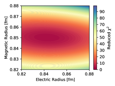
Figure 2: Reduced $\chi^{2}$, Eq. (2), as a function of $r_{E}^{p}$ and $r_{M}^{p}$, after minimization with respect to the normalization parameters.

To estimate the uncertainties of the extracted radii, we use the criterion $\Delta\chi^{2}$ = 2.7 to determine the 68% confidence interval, corresponding to the simultaneous estimation of two independent parameters. The uncertainties of the physical parameters $r_{E}^{p}$ and $r_{M}^{p}$ are affected also by the statistical fluctuations of the normalization parameters $\Lambda_{k}$; we have estimated the total statistical uncertainties using a bootstrap method and found them to be very close to the uncertainties of $r_{E}^{p}$ and $r_{M}^{p}$ one would obtain from the variation of the reduced $\chi^{2}$, obtained after minimization with respect to $(\Lambda_{1},...,\Lambda_{N_{\rm set}})$. In the final uncertainty we also include the theoretical uncertainty of the DI$\chi$EFT FFs (see below) Alarcón et al. (2019).

III Results

In the fit we include the cross section data up to a maximum momentum transfer, $Q^{2}<Q^{2}_{\rm max}$. Suitable values of $Q^{2}_{\rm max}$ are determined by considering the balance of experimental and theoretical uncertainties and the sensitivity of the cross sections to the model parameters $r_{E}^{p}$ and $r_{M}^{p}$ Alarcón et al. (2019). Our standard fit uses $Q^{2}_{\rm max}=0.5$ GeV² and includes 1285 of the 1422 Mainz A1 data points. The overall quality of the description of the experimental cross sections is shown in Fig. 1 (the plots show also the data at $Q^{2}>Q^{2}_{\rm max}$, which were not included in the fit). One sees that all features of the kinematic dependence of the data (with the floating normalization determined by the fit) are reproduced by the theoretical model. The reduced $\chi^{2}$ profile in the physical parameters $r_{E}^{p}$ and $r_{M}^{p}$, obtained after minimization with respect to the normalization parameters, is shown in Fig. 2. One observes that the variations of $\chi^{2}$ in $r_{E}^{p}$ and $r_{M}^{p}$ are approximately independent, and that clear minima are obtained in both parameters. Minimizing with respect to the radii, we extract $r_{E}^{p}=0.842\pm 0.002$ fm and $r_{M}^{p}=0.850\pm 0.001$ fm with a reduced $\chi^{2}$ of 1.39.

To test the robustness of the results we have performed fits with different values of $Q^{2}_{\rm max}$ and found little effect on the extracted radii. In fact, using the entire Mainz A1 data set up to $Q^{2}_{\rm max}=1$ GeV² gives $r_{E}^{p}=0.843\pm 0.002$ fm and $r_{M}^{p}=0.850\pm 0.001$ fm with a reduced $\chi^{2}$ of 1.43. This shows that the theoretical model (evaluated with the “best” value of the radii) accurately describes the $Q^{2}$ dependence of the data over the entire range considered here.

As a further test we have performed fits to the rebinned version of the Mainz A1 data of Ref. Lee et al. (2015), where the original data sets are rescaled to a common normalization using empirical functional forms, including the effects on the random uncertainties. The fit with $Q^{2}_{\rm max}=0.5$ GeV² uses 569 of the 658 rebinned data points and gives radii $r_{E}^{p}=0.840\pm 0.002$ fm and $r_{M}^{p}=0.849\pm 0.001$ fm with a reduced $\chi^{2}$ of 1.07, in good agreement with our fit to the original data. Extending $Q^{2}_{\rm max}$ to include all the rebinned data we obtain $r_{E}^{p}=0.841\pm 0.003$ fm and $r_{M}^{p}=0.849\pm 0.001$ fm with a reduced $\chi^{2}$ of 1.10, showing similar stability the fit to the original data. Overall, the tests show that the extracted radii are not sensitive to the choice of data sets used in the fits.

The Jefferson Lab PRad experiment has reported a new measurement of the electron-proton elastic cross section down to $Q^{2}\sim 10^{-4}$ GeV², significantly extending the reach of earlier measurements Xiong et al. (2019). We have performed a fit including the PRad data in addition to the Mainz A1 data and found no change in the extracted $r_{E}^{p}$ and $r_{M}^{p}$ within uncertainties. This happens because the DI$\chi$EFT model naturally describes the $Q^{2}$ dependence of the low-$Q^{2}$ data, with the same value of $r_{E}^{p}$ as favored by the higher-$Q^{2}$ data Alarcón et al. (2019); this was also observed in the analysis of Ref. Horbatsch (2019). Note that the low-$Q^{2}$ data are sensitive mostly to $r_{E}^{p}$, and that our present extraction of $r_{M}^{p}$ requires us to include data up to $Q^{2}\sim 0.5$ GeV².

In our assessment of the errors of the extracted radii we must include also the intrinsic theoretical uncertainty of the DI$\chi$EFT model. This refers to the uncertainty in the predictions for $G_{E}^{p}$ and $G_{M}^{p}$ for given values of $r_{E}^{p}$ and $r_{M}^{p}$, which results from the modeling of the high-mass states in the dispersion integral (effective poles) and was estimated in Ref. Alarcón et al. (2019). Performing fits with different values of the effective pole mass we estimate the effect on the extracted radii as $\sim$ $\pm$0.010 fm for both $r_{E}^{p}$ and $r_{M}^{p}$; the interval should be regarded as the “full plausible range” of the theoretical uncertainty. Our final results for the extracted radii are thus $r_{M}^{p}$ = 0.850 $\pm$0.001 (fit 68%) $\pm$0.010 (theory full range) fm and $r_{E}^{p}$ = 0.842 $\pm$0.002 (fit 68%) $\pm$0.010 (theory full range) fm.

IV Discussion

Several aspects of our method and results merit further discussion. In our theory-based extraction method the main impact on the radii comes from the data at “higher” $Q^{2}\sim$ 0.1–0.5 GeV² (see Fig. 2 and Ref. Alarcón et al. (2019)). One observes that the magnetic radius is actually better determined than the electric one (see Fig. 2), because the cross section at the “higher” $Q^{2}$ is dominated by the contribution of the magnetic FF. In contrast, in methods based on the $Q^{2}\rightarrow 0$ extrapolation the cross section is always dominated by the electric FF, rendering extraction of the magnetic radius extremely difficult. Our method therefore offers principal advantages for the analysis of the proton’s magnetic structure.

The results of our analysis validate previous results for the proton magnetic radius $\sim$0.85 fm, obtained using dispersive fits of the earlier world data; see Ref. Belushkin et al. (2007) and references therein. They disagree with the results obtained from various empirical fits of the Mainz A1 data Bernauer et al. (2010); Lee et al. (2015). This indicates that the observed discrepancies are due to the extraction methods (analyticity, correlations between $Q^{2}$ regions from dispersion relations) rather than the different data sets.

The values of the electric and magnetic radii extracted from the data are very close. While this may be accidental, it is qualitatively consistent with the nonrelativistic quark model picture (independent particle motion in an $L=0$ orbital, no spin-orbit interactions). Using our method we can also determine the proton’s transverse charge and magnetization radii, which refer to the relativistic representation of the FFs in terms of transverse densities and can be related to the generalized parton distributions Miller (2019); Diehl (2003); Belitsky and Radyushkin (2005); Boffi and Pasquini (2007). The derivatives at $Q^{2}=0$ of the Dirac and Pauli FFs, $F_{1}^{p}$ and $F_{2}^{p}$, are related to those of the electric and magnetic FFs by [$\kappa^{p}\equiv F_{2}^{p}(0)=\mu^{p}-1$ is the anomalous magnetic moment, $m$ is the proton mass]

$$\frac{dF_{1}^{p}}{dQ^{2}}(0) =\frac{dG_{E}^{p}}{dQ^{2}}(0)+\frac{\kappa^{p}}{4m^{2}},$$ (4)

$$\frac{1}{\kappa^{p}}\frac{dF_{2}^{p}}{dQ^{2}}(0) =\frac{1}{\kappa^{p}}\left[\frac{dG_{M}^{p}}{dQ^{2}}(0)-\frac{dG_{E}^{p}}{dQ^{2}}(0)\right]-\frac{1}{4m^{2}}.$$ (5)

In the transverse density representation these derivatives determine the mean squared transverse radii of the distributions of charge and magnetization in the proton Miller (2019),

$$-4\frac{dF_{1}^{p}}{dQ^{2}}(0)=\langle b^{2}\rangle_{1}^{p},\hskip 20.00003pt-\frac{4}{\kappa^{p}}\frac{dF_{2}^{p}}{dQ^{2}}(0)=\langle b^{2}\rangle_{2}^{p}.$$ (6)

Equations (1) and (4)–(6) linearly relate $\langle b^{2}\rangle_{1}^{p}$ and $\langle b^{2}\rangle_{2}^{p}$ to $(r_{E}^{p})^{2}$ and $(r_{M}^{p})^{2}$. Using the results of our fit, we obtain $\langle b^{2}\rangle_{1}=0.394\pm 0.002$ (fit 68%) $\pm 0.011$ (theory full range) fm² and $\langle b^{2}\rangle_{2}=0.531\pm 0.002$ (fit) $\pm 0.019$ (theory) fm². It is interesting to note that, if one neglected the small difference between the extracted electric and magnetic radii and set $(r_{E}^{p})^{2}=(r_{M}^{p})^{2}$, the transverse charge and magnetization radii would be related as

$$\langle b^{2}\rangle_{2}^{p}-\langle b^{2}\rangle_{1}^{p}=\mu^{p}/m^{2}\hskip 20.00003pt[\textrm{if $(r_{E}^{p})^{2}=(r_{M}^{p})^{2}$}],$$ (7)

i.e., the difference would be entirely proportional to the proton magnetic moment. Equation (7) is the partonic expression of the approximate equality of the electric and magnetic radii.