Inner Boundary Condition in Quasi-Lagrangian Simulations of Accretion Disks

Abstract

In simulations of viscously evolving accretion disks, the inner boundary condition is particularly important. If treated incorrectly, it induces incorrect behavior very quickly, because the viscous time is shortest near the inner boundary. Recent work has determined the correct inner boundary in Eulerian simulations. But in quasi-Lagrangian simulations (e.g., SPH, moving mesh, and mesh-less), where the inner boundary is modeled by removing mass within a finite zone, the inner density profile typically becomes anomalously depleted. Here we show how the boundary condition should be applied in such codes, via a simple modification of the usual approach: when one removes mass, one must speed up the remaining material so that the disk’s angular momentum is unchanged. We show with both 1D and 2D moving-mesh (AREPO) simulations that this scheme works as desired in viscously evolving disks. It produces no spurious density depletions and is independent of the mass removal rate, provided that the disk is adequately resolved and that the mass removal rate is not so extreme as to trigger instabilities. This “torque-free” mass removal technique permits the use of quasi-Lagrangian codes to simulate viscously evolving disks, while including a variety of additional effects. As an example, we apply our scheme to a 2D simulation of an accretion disk perturbed by a very massive planet, in which the disk is evolved to viscous steady state.

1 Introduction

In simulating accretion disks, it is common to adopt an inner boundary that lies far outside of the true disk inner edge. This allows the computationally expensive—and often uncertain—dynamics of the innermost regions to be avoided. In this Letter, we work out the correct inner boundary condition, such that a disk with a large inner boundary mimics one with a boundary further in. We then show how it may be applied in a simple way to quasi-Lagrangian codes. We focus on a viscously evolving disk that is perturbed by an embedded planet, but discuss some other applications in §4.

Since the viscous time decreases inwards (Lynden-Bell & Pringle, 1974), an incorrect inner boundary condition can quickly lead to an incorrect density profile in the inner parts of the simulation—long before the density in the vicinity of the planet can evolve viscously. But that short inner viscous time also suggests the principle that should be applied to determine the correct inner boundary: that the inner parts of the disk should be locally in steady-state, with a radially independent mass accretion rate.

In Eulerian simulations of accretion disks, inner boundary conditions may be applied at a fixed spatial location, as done in our previous work Dempsey et al. (2020, hereafter DLL20); see also §2.3. But in quasi-Lagrangian simulations, it is more natural to remove mass within an inner zone, as has been done in smoothed particle hydrodynamics (SPH; e.g., Bate et al., 1995); in meshless codes (e.g., Hopkins, 2017); and in structured and unstructured moving-mesh codes (Farris et al., 2014; Muñoz & Lai, 2016). In the aforementioned papers, mass is removed without changing the velocity of the remaining material. This method, as shown below, artificially exerts a torque on the disk, which leads to an incorrect inner density profile within the computational domain.

Artifacts induced by artificial mass removal have recently given rise to a controversy in the context of disks with embedded stellar binaries. Tang et al. (2017) claimed that the inner mass removal procedure can be crucial for determining the sign of the torque on the binary. If that were true, the surprising result that accreting binaries expand (Muñoz et al., 2019, 2020) could be an artifact of incorrect mass removal. While follow-up studies (Moody et al., 2019; Duffell et al., 2019) were unable to confirm the Tang et al. claim, it is still desirable to devise mass removal methods that introduce no artifacts at all. In this work, we describe and implement such a method in the moving-mesh code AREPO (Springel, 2010).

2 Torque-free Inner Boundary

2.1 Why the inner boundary should be torque-free

The 1D equations of mass and angular momentum conservation for a viscous accretion disk, in the absence of a planet, are (Lynden-Bell & Pringle, 1974)

$$2\pi r\frac{\partial\Sigma}{\partial t} - \frac{\partial\dot{M}}{\partial r}=0\ ,$$ (1)

$$2\pi r\frac{\partial\Sigma\ell}{\partial t} + \frac{\partial}{\partial r}\left(F_{\nu}-\dot{M}\ell\right)=0\ ,$$ (2)

where $\ell=r^{2}\Omega(r)$ is the specific angular momentum; $\Omega\propto r^{-3/2}$ is the Keplerian angular speed i.e., ignoring the pressure correction; $\dot{M}(r)$ is the radial mass flux; and $F_{\nu}=3\pi\nu\Sigma\ell$ is the viscous angular momentum flux, where $\nu$ is the kinematic viscosity. One may solve the above equations for

$$\dot{M}=\left(\frac{d\ell}{dr}\right)^{-1}\frac{\partial F_{\nu}}{\partial r}\ ,$$ (3)

and that expression may then be inserted into equation (1), yielding a diffusive partial differential equation for $\Sigma$.

The fact that the viscous time decreases inwards implies that, if $\Sigma$ at some fiducial radius is varying due to viscous evolution, then the $\Sigma$ at much smaller radii can be determined by setting $\partial_{t}=0$ in the above equations. Doing so, we find

$$\dot{M} = {\rm const.\ in\ }r\ ,$$ (4)

$$\Delta T \equiv F_{\nu}-\dot{M}\ell={\rm const.\ in\ }r\ .$$ (5)

The quantity $\Delta T$ is the net torque, i.e., it is the sum of two angular momentum fluxes: the (outwards) viscous flux and the (inwards) advective flux. As a result, the surface density far inside of the fiducial radius is given by

$$\Sigma=\frac{\dot{M}}{3\pi\nu}+\frac{\Delta T}{3\pi\nu\ell}\ .$$ (6)

As is well-known, the $\Sigma$ profile in a steady-state disk is a sum of two terms, with two arbitrary constants, $\dot{M}$ and $\Delta T$ (Lynden-Bell & Pringle, 1974).

The second term in Equation (6) falls with distance faster than the first. Therefore, while these two terms are comparable at the disk’s true inner edge (Lynden-Bell & Pringle, 1974), the second one becomes subdominant further out. Consequently, in order to apply an inner boundary condition far beyond the true inner edge, one should enforce $\Delta T=0$ at the boundary. We call this a “torque-free” boundary.

For future reference, we refer to the $\Sigma$ solution with $\Delta T=0$ as the ZAM (“zero angular momentum flux”) solution, i.e.,

$$\Sigma_{Z}=\frac{\dot{M}}{3\pi\nu}\ .$$ (7)

2.2 Implementation of torque-free inner boundary

A torque-free inner boundary is simple to implement when solving the 1D equations with a finite difference method. Substituting Equation (3) into the relation $F_{\nu}-\dot{M}\ell=0$ yields a relationship between $F_{\nu}$ and $\partial_{r}F_{\nu}$, and hence between $\Sigma$ and $\partial_{r}\Sigma$, that can be applied at the inner boundary (a Robin boundary condition). Essentially the same technique can also be implemented in 2D Eulerian hydrodynamical codes with little difficulty, e.g., with FARGO3D (Benítez-Llambay & Masset, 2016), as done in DLL20.

On the other hand, in quasi-Lagrangian codes it is more natural to remove mass throughout an extended zone. In most previous work, mass is removed either by eliminating entire particles (e.g., Bate et al., 1995), or by draining mesh cells, reducing their mass and momenta by the same fraction (e.g., Farris et al., 2014; Muñoz & Lai, 2016). In both cases, the velocity of the remaining fluid is left unchanged. This technique, which we call “naive mass removal,” violates the torque-free inner boundary condition, because when momentum is removed, an angular momentum sink term must be added to Equation (2). As a result, in viscous steady state the value of $\Delta T$ at the outer edge of the mass removal zone (which we denote $r_{0}$) will be non-zero. Note that $r_{0}$ corresponds to what we have been calling the inner boundary, because it is the inner boundary of the region where the physics is properly modelled (i.e., no mass removal.) Of course, the region inside of $r_{0}$ (the mass removal zone) is still modeled with the code.

One may enforce $\Delta T=0$ at $r_{0}$ by ensuring that there are no sources or sinks of angular momentum in the mass removal zone, so that Equation (2) remains unchanged. In quasi-Lagrangian codes, this can be accomplished by increasing the azimuthal velocity of a mesh cell every time its mass is reduced, such that its angular momentum is preserved. We call this technique “torque-free mass removal,” and we shall investigate it in more detail in the remainder of this Letter.

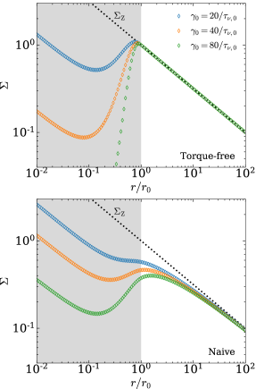
Figure 1: Steady-state profiles from 1D simulations of torque-free (top) and naive (bottom) mass removal. Three values of $\gamma_{0}$ are shown, with values in the inset in units of $\tau_{\nu,0}$, which is the viscous time at $r=r_{0}$.

2.3 Torque-free versus naive mass removal in 1D

It is instructive to demonstrate the difference between torque-free and naive mass removal in 1D. Mass removal can be modeled in 1D simulations by modifying Equation (1) to

$$2\pi r\frac{\partial\Sigma}{\partial t}-\frac{\partial\dot{M}}{\partial r}=-\gamma(r)2\pi r\Sigma,$$ (8)

where $\gamma$ is a mass removal function that vanishes for $r\geq r_{0}$. For $r<r_{0}$, we choose the form

$$\gamma(r)=\gamma_{0}(1-r/r_{0})^{2}$$ (9)

which rises to $\gamma_{0}$ at the origin; here, $\gamma_{0}$ is a constant with units of inverse time.

To model torque-free mass removal, we evolve Equations (2) and (8) with a finite difference code. We initialize with the ZAM value for $\Sigma$, set the outer boundary condition to have fixed $\dot{M}$ (via Equation (3) with $\dot{M}$ specified), and run until the $\Sigma$ profile reaches steady state. We also set $\nu={\rm const}\times r^{1/2}$ and adopt the aforementioned Robin inner boundary condition at $r=0.01r_{0}$.

The result is shown in Figure 1 (top panel), for three values of $\gamma_{0}$. We see that torque-free mass removal produces the correct (ZAM) profile at $r>r_{0}$, independent of $\gamma_{0}$, as desired. Inside of $r_{0}$, the depression in $\Sigma$ increases with increasing $\gamma_{0}$. As discussed below, in 2D simulations one typically wishes to choose $\gamma_{0}\sim 10$-$100/\tau_{\nu,0}$, where $\tau_{\nu,0}$ is the viscous time (i.e., $r^{2}/\nu$) at $r_{0}$.

The bottom panel of Figure 1 contrasts what happens with naive mass removal. For that panel we proceed as before, except that we add the sink term $-\gamma 2\pi r\Sigma\ell$ to Equation (2), for reasons discussed above. We infer from the plot that naive mass removal depresses the density profile outside of $r=r_{0}$, relative to the correct $\Sigma_{Z}$. This depression worsens as $\gamma_{0}$ increases. In general, deviations from $\Sigma_{Z}$ indicate that the inner edge of the disk is being incorrectly torqued – in this case due to the mass removal algorithm.

3 Torque-Free Mass Removal in AREPO

We run 2D quasi-Lagrangian simulations with AREPO (Springel, 2010; Pakmor et al., 2016), which solves the Navier-Stokes equations (Muñoz et al., 2013) on a moving mesh. The mesh is constructed from a Voronoi tessellation of points that move with the fluid. Our setup is broadly similar to that of Muñoz et al. (2014): the viscous stress tensor is implemented via a kinematic shear viscosity, parametrized with the Shakura & Sunyaev (1973) $\alpha$ prescription, and the equation of state is locally isothermal with constant aspect ratio. Here, we use $\alpha=H/r=0.1$. The central potential is softened inside of $r_{0}$ with a spline function (Springel et al., 2001) such that outside of $r_{0}$ the potential is exactly Keplerian. See Appendix A for further computational details, including a resolution study.

We implement torque-free mass removal as described in §2.2. At every timestep, we reduce the mass of a cell at the rate given by Equation (9), while preserving the cell’s angular momentum, which has the effect of boosting the cell’s azimuthal velocity. Our initial $\Sigma$ profile has a cavity out to $3r_{0}$, and an outer exponential cutoff at $r=100r_{0}$.

In Figure 2 (top panel), we compare the AREPO 2D solutions to those obtained by solving the 1D equations, for $\gamma_{0}=20/\tau_{\nu,0}$ and $=40/\tau_{\nu,0}$. We find excellent agreement between the two methods at $r>r_{0}$. The simulations in the figure have been run to a time equal to 800 orbits at $r_{0}$, which corresponds to a viscous time at $r\approx 3r_{0}$. But the $\Sigma$ profiles cease to evolve visibly at times $\gtrsim$ 400 orbits at $r_{0}$. There is a modest discrepancy between AREPO and 1D results for the case with lower $\gamma_{0}$ due to the larger discretization errors at smaller $r$ (see also below).

The bottom panel shows a similar comparison, but for naive mass removal—both in AREPO and in the 1D code. As before, the results of the two codes agree at $r>r_{0}$. For the simulations shown, naive mass removal gives a noticeable density depletion relative to the ideal (ZAM) solution out to $r\sim 3$–5$r_{0}$. Similar depressions are often seen in SPH simulations of protoplanetary disks that implement naive mass removal via a sink particle (e.g., Hubber et al., 2018; Price et al., 2018), but are also apparent in simulations using other methods (e.g., Krumholz et al., 2004; Tang et al., 2017).

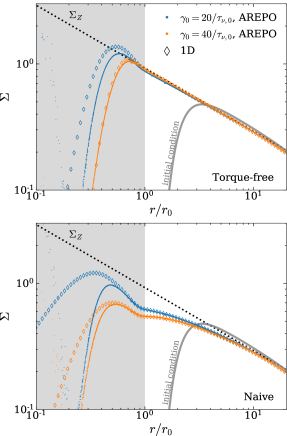
Figure 2: Surface densities resulting from torque-free mass removal (top) and naive mass removal (bottom). We plot the density of each cell in AREPO with a dot. The fact that there is little scatter, except at very small $r$, indicates that the $\Sigma$ profile is very axisymmetric. The 1D profiles here differ slightly from those in Figure 1 within the mass removal zone because of the softened potential used here.

How should one choose $\gamma_{0}$? There are two competing considerations. If $\gamma_{0}$ is too small, then too little mass is removed, obviating the reason for using mass removal in the first place. Conversely, if $\gamma_{0}$ is too large, we find that the disk develops non-axisymmetries. For example, a simulation with $\gamma_{0}\gtrsim 80/\tau_{\nu,0}$ but otherwise the same as Figure 2 develops an $m=2$ pattern at $r_{0}$ (see Appendix A.2). We have not identified the origin of the instability, but note that for large $\gamma_{0}$ the density gradient becomes large near $r_{0}$, and hence the disk can experience Rayleigh (Chandrasekhar, 1961) or Rossby wave instabilities (Li et al., 2000; Lovelace et al., 1999).

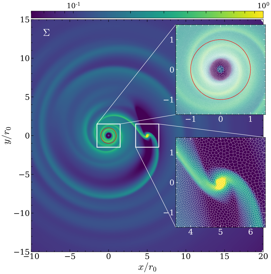
Figure 3: Disk surface density for a planet with mass ratio $5\times 10^{-3}$ after the disk has reached viscous steady state. The red circle is at $r=r_{0}$. The insets around the star and the planet show the Voronoi mesh, which is refined with mass-refinement around the planet, and cellsize-refinement around the star (see Appendix A.1).

4 Steady-state Disk perturbed by a Planet

We apply torque-free mass removal to the situation studied in DLL20: a planet is placed on a fixed orbit within a viscous disk, and then the disk is evolved long enough to reach viscous steady state beyond the planet’s orbit.

We take the planet’s mass to be $5\times 10^{-3}$ times that of the star, and place it on a circular orbit at $5r_{0}$. We set the disk parameters to be the same as in Figure 2, with $\gamma_{0}=40/\tau_{\nu,0}$, and work in the stellar-centric frame by including an indirect potential. We run the simulation with AREPO, using torque-free mass removal, to a time of $\sim 1,100$ planetary orbits, which is the viscous time at $\sim 18r_{0}$.

Figure 3 shows a snapshot of the resulting surface density and Voronoi mesh. The planet excites spiral density waves, which torque the gas, altering the $\Sigma$ profile (Goldreich & Tremaine 1980; Lunine & Stevenson 1982; Kanagawa et al. 2017; DLL20). Note that we do not employ wave-killing in the simulation (e.g., de Val-Borro et al., 2006). Despite that, the waves launched by the planet do not reflect off of the inner boundary, as evidenced by the absence of leading spiral arms in the figure.

Figure 4 (top panel) shows the $\Sigma$ profile of the disk. The planet is massive enough to open a modest gap around its orbit. Furthermore, $\Sigma$ remains below the ZAM profile (Equation 7) nearly to $r_{0}$, due to the long reach of the spiral waves (DLL20).

For comparison, we show in the top panel of Figure 4 the result from an Eulerian simulation, done with FARGO3D. The setup is very similar to the simulations in DLL20. The grid is logarithmically-spaced in radius, and extends from $r=[0.5,35]r_{0}$ with $N_{r},N_{\phi}=(340,502)$. It also includes a wave-killing zone inside of $r_{0}$. As seen in the figure, the agreement between FARGO3D and AREPO is excellent.

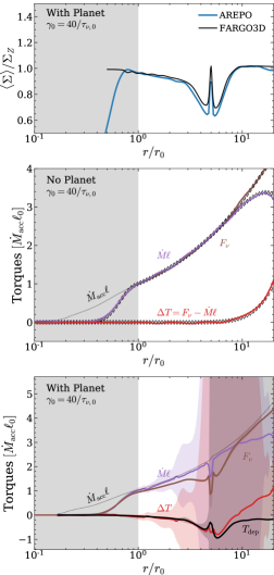
Figure 4: The top panel shows the azimuthally averaged $\Sigma$ profile for our planet runs with AREPO (blue line) and FARGO3D (black line); $\Sigma$ is scaled to the ZAM profile (Equation 7), taken at an $\dot{M}$ equal to the one measured in the simulations ($=\dot{M}_{\rm acc}\approx 0.35\times 3\pi\nu_{0}\ell_{0}$). The middle panel shows the torques in the planet-less AREPO simulation from Figure 2 (colored lines), as well as those from the 1D code (diamonds). The bottom panel shows the torques in the AREPO simulation from the top panel, time-averaged over $50$ planet orbits. We describe how we compute the azimuthally averaged torques and $\Sigma$ profile in Appendix A.3.

We turn now to examining the torques in the AREPO simulation. One of the key quantities in studying planet-disk interaction is the value of the net torque $\Delta T$ (Equation 5) far beyond the planet’s orbit. Recall that $\Delta T$ is one of the two constants in a steady-state planet-less disk. Therefore far beyond the planet’s orbit $\Delta T$ should be spatially constant in viscous steady state. The value of that constant determines both the planet’s migration rate and the “pileup” of material outside of its orbit (DLL20).

To set the stage for the torques in the planet simulation, we first show in the middle panel of Figure 4 what happens without a planet, in one of the simulations from Figure 2. We see that $\Delta T$ vanishes at $r_{0}$ and inwards, demonstrating that our torque-free mass removal procedure is behaving as intended. In addition, $\Delta T$ remains negligibly small out to $r\sim 10r_{0}$, demonstrating that the disk is in viscous steady state out to that radius. We also show in the figure the two components of $\Delta T$, i.e., $F_{\nu}$ and $\dot{M}\ell$, and these are both equal to $\dot{M}_{\rm acc}\ell\propto r^{1/2}$ throughout the physical part of the domain that is in steady state, as required by the planet-less viscous steady state solution (§2.1); here, $\dot{M}_{\rm acc}$ is the rate at which mass is artificially removed within the inner zone of the simulation.

The torques in the AREPO planet simulation are shown in the bottom panel of Figure 4, where they are time-averaged over $50$ planetary orbits, and the $1$-$\sigma$ deviations are shown as shaded regions. We observe again that $\Delta T$ is negligibly small at $r_{0}$, as required, and remains small until near the planet’s orbit. One may note that $\Delta T$ does not reach a constant value at large $r$, because the simulation is not quite in viscous steady state there (similar to the middle panel). But given that the constant’s value is so important, we display it in a different way: we consider $T_{\rm dep}(r)$, which is the torque deposited into the disk by spiral waves that have been launched by the planet (DLL20). In viscous steady state with a planet, Equation (5) is modified to $\Delta T(r)=T_{\rm dep}(r)$, i.e., the net torque in the disk must equal that provided by the deposition of spiral wave torque. The figure shows $T_{\rm dep}(r)$, which we measure by combining the torque required to excite the waves with the torque transported by the waves (as explained in e.g., Kanagawa et al. 2017; DLL20).

We see that $\Delta T\approx T_{\rm dep}$ within $\sim 10r_{0}$, as required by viscous steady state. In addition, the total torque deposited into the disk, i.e., $T_{\rm dep}$ at ${r\gg r_{\rm pl}}$, is very small in absolute value relative to $\dot{M}_{\rm acc}\ell_{0}$. Moreover, further investigation shows that it oscillates with small amplitude over time, likely due to the disk being slightly eccentric (Dempsey et al., in prep). We conclude that for this setup the planet migration rate is very slow, and moreover there is a negligibly small pileup outside of the planet’s orbit.

5 Summary and Discussion

Our main results are as follows:

• The inner boundaries of accretion disks should be designed to ensure that they are torque free ($\Delta T=0$). Otherwise, the density profile beyond the boundary will be incorrect. Conversely, one may infer that boundary-induced density depressions found in many quasi-Lagrangian simulations are due to an artificial torquing of the disk by the mass removal algorithm.

• We introduced a simple method to ensure a torque-free inner boundary in quasi-Lagrangian codes that use mass removal schemes: the azimuthal velocity of the material remaining after mass removal is increased to avoid changing the angular momentum. Once the angular momentum is properly handled, further details of mass removal have negligible impact on the disk’s behavior.

• We implemented this mass removal in AREPO, showing that it produced the desired behavior both in planet-free disks, and in a disk with a planet—allowing one to determine the total torque of the planet on the disk, $\Delta T$.

Our mass removal algorithm is similar to the angular momentum-preserving sinks of Krumholz et al. (2004). But the disks in Krumholz et al. (2004) do not achieve the ZAM solution outside the accretion zone (cf. their Figures 7-8). Instead, they exhibit an “evacuation zone” that grows in time, implying that their algorithm is not truly torque-free. We hypothesize that this might be caused by inadequate resolution.

Bate et al. (1995) introduced a fix to correct for the discontinuity in density across the inner boundary present in SPH simulations. Their fix appears to alleviate at least part of the boundary-induced density depletion (see their Figure 2). However, it does not ensure that $\Delta T=0$ in the inner parts of the simulation.

Although we have focused on disks nearly in viscous steady state, inner boundaries should almost always be torque-free, even for time-dependent disks. That is because the viscous timescale is shortest in the inner regions, and so even if the disk is evolving viscously, the innermost regions should be effectively in steady state. The only exception we see is when one wishes to model the effect of a true inner boundary—e.g., due to a stellar magnetosphere. Nonetheless, we do not claim that previous simulations with non-torque-free inner boundaries are invalid. Far away from such a boundary, the boundary’s effect may indeed be ignored.

We foresee a number of applications. The planet simulation considered here may be extended to other cases, including binary stars and more realistic disks. For that simulation, FARGO3D was sufficient—indeed, it is around five times as fast as AREPO . But for cases where the flow becomes strongly non-Keplerian, the orbital advection algorithm used in FARGO3D becomes much less efficient. Additional applications include modeling of the circumplanetary/circumsecondary disk region and the evolution of warps. Regarding the last application, we foresee no great difficulty in extending our 2D method to 3D —although the requirements for our method to work in 3D have yet to be examined.

Appendix A AREPO Simulation Details

A.1 Refinement Criteria

To ensure that there is adequate spatial resolution, we make use of two different cell refinement/derefinement criteria. The first, which becomes most important in the vicinity of the planet, is the default mass-based resolution in AREPO. We specify a target cell mass, $m_{\rm target}$. If a cell has a mass outside of the range $m_{\rm cell}=[0.5m_{\rm target},2m_{\rm target}]$, that cell is either split or merged with surrounding cells so that the resulting mass falls within the specified range. In our simulation with a planet, we smoothly decrease $m_{\rm target}$ by a factor of 300 in the Hill sphere of the planet.

Our second refinement criteria, which becomes important in the vicinity of the star, and is used in conjunction with the mass based criterion, is cell size based and enforces a minimum number of cells in the azimuthal direction. We specify a target cell radius, $r_{\rm target}$, that is equal to $2\pi r/N_{\phi}$, where $N_{\phi}$ is the desired number of cells in the azimuthal direction. If a cell has a radius outside of the range $r_{\rm cell}=[0.5r_{\rm target},2r_{\rm cell}]$, it is either split or joined with neighboring cells until the cell radius falls within our specified range. To ensure a smooth transition in cell size towards the star we lower the $N_{\phi}$ from the nominal target value as $(r/r_{0})^{3}$ inside $r_{0}$.

A.2 Resolution Requirements

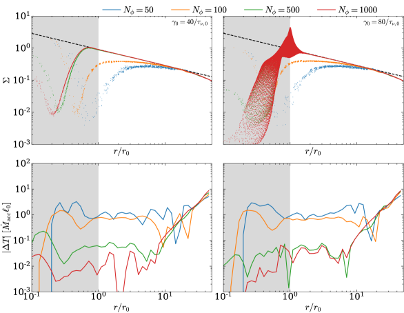
Figure 5: The resolution requirements for torque-free mass removal in planet-less AREPO simulations. The two left panels show the case with $\gamma_{0}=40/\tau_{\nu,0}$. In the top-left panel, the dots show $\Sigma$ within every cell, in which case non-axisymmetries are evident as the spread in points at a given $r$. We see that one requires $N_{\phi}\gtrsim$a few hundred for the steady state profile to match the ZAM solution (dashed line). The lower-left panel shows the net torque. We see that even for the crudest resolution $\Delta T$ is nearly spatially constant. The error in the top-left panel is therefore due to the errors within the mass removal zone (which can likely be corrected with a better treatment of that zone). The right panels show a case with $\gamma_{0}$ twice as large. In this case, the disk becomes highly non-axisymmetric at a resolution $N_{\phi}=500$; surprisingly, however, that does not much affect the behavior further out.

We explore different values of $N_{\phi}$ in Figure 5 for planet-less disks, with two different $\gamma_{0}$ values. We conclude that $\gamma_{0}=40/\tau_{\nu,0}$ and $N_{\phi}=1000$ (the values used in the body of this Letter) suffice to accurately simulate the disk.

A.3 Flux measurements

In Figure 4 we show the azimuthally-averaged steady-state torques. Computing these azimuthal averages is a non-trivial task in AREPO as the cells are not on a cylindrical grid. During a simulation, we add a cell’s content (be it mass, viscous flux, $\dot{M}$, etc.) into finely spaced radial bins. For each binned quantity, we compute the cumulative radial integral across the domain, and then compute the numerical derivative on a coarser grid. This leaves us with an estimate for the azimuthal average of each quantity. For the planet-less simulations we use logarithmically spaced bins with width $\Delta\ln r_{\rm bin}\approx 0.001$ and evaluate the numerical derivatives with a radial grid with spacing $\approx 0.14$. For the planet simulation we evaluate the numerical derivatives with a finer radial grid with spacing $\approx 0.034$.

References

- Bate et al. (1995) Bate, M. R., Bonnell, I. A., & Price, N. M. 1995, MNRAS, 277, 362
- Benítez-Llambay & Masset (2016) Benítez-Llambay, P., & Masset, F. S. 2016, ApJS, 223, 11
- Chandrasekhar (1961) Chandrasekhar, S. 1961, International Series of Monographs on Physics
- de Val-Borro et al. (2006) de Val-Borro, M., Edgar, R. G., Artymowicz, P., et al. 2006, MNRAS, 370, 529
- Dempsey et al. (2020) Dempsey, A. M., Lee, W.-K., & Lithwick, Y., 2020, ApJ, 891, 108
- Duffell et al. (2019) Duffell, P. C., D’Orazio, D., Derdzinski, A., et al. 2019, arXiv, arXiv:1911.05506
- Farris et al. (2014) Farris, B. D., Duffell, P., MacFadyen, A. I., & Haiman, Z. 2014, ApJ, 783, 134
- Goldreich & Tremaine (1980) Goldreich, P., & Tremaine, S. 1980, ApJ, 241, 425
- Hopkins (2017) Hopkins, P. F. 2017, arXiv, arXiv:1712.01294
- Hubber et al. (2018) Hubber, D. A., Rosotti, G. P., & Booth, R. A. 2018, MNRAS, 473, 1603
- Kanagawa et al. (2017) Kanagawa, K. D., Tanaka, H., Muto, T., & Tanigawa, T. 2017, PASJ, 69, 97
- Krumholz et al. (2004) Krumholz, M. R., McKee, C. F., & Klein, R. I. 2004, ApJ, 611, 399
- Li et al. (2000) Li, H., Finn, J. M., Lovelace, R. V. E., & Colgate, S. A. 2000, ApJ, 533, 1023
- Lovelace et al. (1999) Lovelace, R. V. E., Li, H., Colgate, S. A., & Nelson, A. F. 1999, ApJ, 513, 805
- Lunine & Stevenson (1982) Lunine, J. I., & Stevenson, D. J. 1982, Icarus, 52, 14
- Lynden-Bell & Pringle (1974) Lynden-Bell, D., & Pringle, J. E. 1974, MNRAS, 168, 603
- Moody et al. (2019) Moody, M. S. L., Shi, J.-M., & Stone, J. M. 2019, ApJ, 875, 66
- Muñoz et al. (2014) Muñoz, D. J., Kratter, K., Springel, V., & Hernquist, L. 2014, MNRAS, 445, 3475
- Muñoz & Lai (2016) Muñoz, D. J., & Lai, D. 2016, ApJ, 827, 43
- Muñoz et al. (2020) Muñoz, D. J., Lai, D., Kratter, K., & Miranda, R. 2020, ApJ, 889, 114
- Muñoz et al. (2019) Muñoz, D. J., Miranda, R., & Lai, D. 2019, ApJ, 871, 84
- Muñoz et al. (2013) Muñoz, D. J., Springel, V., Marcus, R., Vogelsberger, M., & Hernquist, L. 2013, MNRAS, 428, 254
- Pakmor et al. (2016) Pakmor, R., Springel, V., Bauer, A., et al. 2016, MNRAS, 455, 1134
- Price et al. (2018) Price, D. J., Wurster, J., Tricco, T. S., et al. 2018, PASA, 35, e031
- Shakura & Sunyaev (1973) Shakura, N. I., & Sunyaev, R. A. 1973, A&A, 24, 337
- Springel (2010) Springel, V. 2010, MNRAS, 401, 791
- Springel et al. (2001) Springel, V., Yoshida, N., & White, S. D. M. 2001, New Astronomy, 6, 79
- Tang et al. (2017) Tang, Y., MacFadyen, A., & Haiman, Z. 2017, MNRAS, 469, 4258