Optimal Multiple Stopping Rule for Warm-Starting Sequential Selection

Abstract

In this paper we present the Warm-starting Dynamic Thresholding algorithm, developed using dynamic programming, for a variant of the standard online selection problem. The problem allows job positions to be either free or already occupied at the beginning of the process. Throughout the selection process, the decision maker interviews one after the other the new candidates and reveals a quality score for each of them. Based on that information, she can (re)assign each job at most once by taking immediate and irrevocable decisions. We relax the hard requirement of the class of dynamic programming algorithms to perfectly know the distribution from which the scores of candidates are drawn, by presenting extensions for the partial and no-information cases, in which the decision maker can learn the underlying score distribution sequentially while interviewing candidates.

I Introduction

Sequential Selection Problems (SSPs) occur in several real-life situations. A common characteristic of such decision processes is that decisions need to be immediate and irrevocable. For instance, at an emergency healthcare unit, patients arrive sequentially seeking for medical help [8]. Other examples are found in kidney exchanges [4], auctions [9], robotic sampling [5], and most straightforwardly in recruitment processes that involve sequential interviews of job-seekers by a decision maker (DM), who immediately takes hiring or rejection decisions [3]. For clarity, we adopt the terminology of the latter problem, e.g. candidates are interviewed, hiring means selecting, firing is deselecting, etc.

In the most well-known SSP, the secretary problem [7, 10], $n\in\mathbb{N}^{*}$ candidates are sequentially interviewed for a single job position, and a hire puts an end to the recruitment process. Its multi-choice extension, also called multiple stopping problem, has been extensively studied [9, 2, 1], and terminates when the desired number of $b\in\mathbb{N}^{*}$ hired have been decided. In the hiring problem [3], the DM’s task is to grow the company as much as possible while keeping maximal the average score of the hired employees; therefore, there is no limit in the number of job positions. The hiring-above-the-mean policy was proposed, which selects a candidate when his score exceeds the average score of the current employees (changes over time). This policy is an efficient and easy to implement, yet notably dependent on the score distribution and sensitive to the quality of the first hires.

What we call as the full-information case, assumes that the distribution from which the scores of candidates are sampled is known to the DM. In [11], dynamic programming is employed to compute the optimal stopping rule for each candidate, i.e. the score threshold to beat in order to be hired. This threshold depends on his arrival time and on the number of jobs positions that remain to be filled.

One important limitation of all the aforementioned settings is that they begin with an empty selection set. The case of performing a selection starting with a set of items at hand was only recently introduced in [6]. There, a preselection is composed of the pre-existing items that can then be replaced, by selecting better items from those that appear sequentially, to produce the final selection. More specifically, the authors present the so-called Warm-starting Sequential Selection Problem (WSSP) where the DM can perform at most one update per job position. This setting can also suit well to multi-round applications where the output of a round is the input of the subsequent one.

The Cutoff-based Cost Minimization algorithm from the same work [6] makes no assumption on the distribution of candidates’ scores. It splits the process into two phases: the learning phase in which the DM learns an acceptance threshold from candidates that are getting rejected by default, and thereafter, the selection phase which uses that threshold to accept or reject from the rest candidates. Despite its biased rule, which is due to the disregard of the early-arriving candidates, the strategy can be efficient and robust to score changes, provided an appropriately set learning phase size.

Important to note, when the score distribution is known, the cutoff-based strategies are not optimal and policies derived from dynamic programming are more suitable. To the best of our knowledge, there exists no such warm-starting strategy in the literature.

Contribution. Inspired by the warm-starting aspect of the WSSP [6], we propose the Warm-starting Dynamic Thresholding (WDT) algorithm that attributes to each incoming candidate a threshold value to beat according to: i) its arrival time, ii) the current number of empty job positions, and iii) the current number of positions occupied by initial employees (i.e. available employees that can be replaced). The threshold value to beat is computed by means of dynamic programming, adapted to the warm-starting scenario. The algorithm is easy to implement and gives each candidate a chance to be hired regardless his arriving time. WDT’s downside lies in the assumption that the score distribution is known. We relax this requirement by first considering the partial information case where the DM only knows the nature of the distribution, and then the no-information case where the threshold is purely rank-based. We show with simulations that the WDT outperforms existing methods in the warm-starting scenario.

II Setting

The Sequential Selection Problem (SSP) of interest is the following: $n\in\mathbb{N}^{*}$ candidates are sequentially interviewed by a decision maker (DM) who has the task of managing a limited budget of $b\in\mathbb{N}^{*}$, $b\leq n$, interchangeable job positions. Initially, $r\leq b$ positions are empty as some employees have become permanently unavailable, while the rest $b-r$ are initially occupied by existing employees that form a set called preselection. Available and unavailable employees constitute a reference set for the DM. Once candidate $j$ arrives, the DM observes his score $S_{j}\in$, which, like all scores, it is assumed to follow a known distribution $f_{S}$. In our notations, an added dot on top of a variable refers to the preselection, e.g. $\dot{\mathbf{S}}=(\dot{S}_{(1)},\dot{S}_{(2)},...,\dot{S}_{(b-r)})$ gives the score of each preselected employee. For convenience, the latter vector is considered to be sorted in decreasing order, i.e. $\dot{S}_{(1)}$ and $\dot{S}_{(b-r)}$ are respectively the best and the worst scores of the preselected employees. Here are the basic rules of the game:

• Each decision (i.e. hire or not) shall be immediate and irrevocable, which means that every position can be assigned (or reassigned) at most once throughout the selection process.

• The DM must at least fill the empty job positions by hiring $r$ candidates.

• Once no empty position is left, the DM can still hire an incoming candidate by removing one of the employees of the preselection from his position (only fire on hire).

The following definition is a score-based adaptation of the Warm-starting Sequential Selection Problem (WSSP) proposed in [6], where here the DM initially knows also the distribution from which candidates’ scores are drawn.

Definition 1

Distribution-aware WSSP is the online selection process described by elements of three categories:
1) Background

$\mathcal{B}=(b,n,f_{S},\dot{\mathbf{S}})$: collection of elements initially at DM’s knowledge or disposition, including:

• $n\in\mathbbm{N}^{*}$: finite number of candidates to appear;

• $b\in\mathbbm{N}^{*}$, $b\leq n$: number of resources;

• $f_{S}$: the distribution generating candidates’ scores;

• $\dot{\mathbf{S}}=(\dot{S}_{(1)},...,\dot{S}_{(b-r)})\in^{b-r}$; $\dot{S}_{(j)}\sim f_{S},\ \forall j$: scores of the preselection.

2) Process

• $\mathbf{S}=(S_{1},...,S_{n})\in^{n}$; $S_{j}\sim f_{S},\ \forall j$: candidates’ scores;

• $\mathbf{A}=(A_{1},...,A_{n})\in\{0,1\}^{n}$: sequence of decisions for candidates, i.e. $A_{j}=1$ if the $j$-th candidate gets hired.

3) Evaluation

• The reward is evaluated at the end of the process by:

  $$\phi_{\mathcal{B}}(\mathbf{S},\mathbf{A})=\sum_{i=1}^{b-r}\dot{S}_{(i)}\dot{A}_{(i),n}+\sum_{j=1}^{n}S_{j}A_{j}\,\,\geq 0,$$ (1)

  where $\dot{A}_{(i),n}\in\{0,\,1\}$ indicating if the $i$-th preselected employee kept his position after $n$ candidate interviews.

The evaluation criterion to maximize is therefore the expectation of the above reward function, $\mathbb{E}[\phi_{\mathcal{B}}(\mathbf{S},\mathbf{A})]$. Note that, since the DM is forced to fill the $b$ positions by the end of the process, it holds: $\sum_{i=1}^{b-r}\dot{A}_{(j),n}+\sum_{j=1}^{n}A_{j}=b$.

III Warm-starting Dynamic Thresholding

Here, we present the Warm-starting Dynamic Thresholding (WDT) method to solve optimally the distribution-aware WSSP of Definition 1. Without loss of generality, we consider non-negative i.i.d. scores $S_{j}\geq 0,\,\forall j$, and that the best- (resp. worst-) skilled individual has the highest (resp. lowest) score.

III-A Threshold-based algorithm

The idea behind the strategy is to find the optimal acceptance threshold $T_{j}\in$ that the $j$-th arriving candidate should beat in order to be hired, $\forall j\in\{1,...,n\}$; see the example of Fig. 2. Note that, in order to be optimal, this threshold must depend on the state of the ongoing selection process. Therefore, we write $T_{j}=T_{j}^{X_{j},Y_{j}}$, where $X_{j}\in\{0,...,r\}$ positions are still empty and $Y_{j}\in\{0,...,b-r\}$ jobs are still occupied by preselected employees, i.e. after $j-1\in\mathbb{N}^{*}$ interviews and while the $j$-th candidate is being interviewed. Using the notations of Definition 1 we get:

$$X_{j}:=\max\left(r-\sum_{i=1}^{j-1}A_{i},\,\,0\right)\,\ \text{and}\,\ Y_{j}:=\sum_{i=1}^{r}\dot{A}_{(i),j}.$$ (2)

To simplify our notations, we omit the dependency of $X_{j}$ and $Y_{j}$ to $j$, and we simply write $X$ and $Y$ to refer to their value at the implied step $j$ of the selection process.

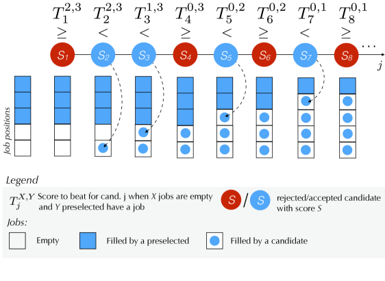
Figure 1: Demonstration of the WDT algorithm. The score of an incoming candidate, $S_{j}$, is compared to an associated acceptance threshold $T_{j}^{X,Y}$​, where $X$ and $Y$ are respectively the current number of empty positions and that of positions occupied by preselected employees. Accepted candidates (blue circle) first fill empty positions and then, if they are competitive enough, take a preselected employee’s positions (e.g. the $5$-th candidate).

Value function. The fundamental question remains how to compute the thresholds optimally. The solution can be found via dynamic programming where the value function, which is the expected value of the regret here, is computed for each possible scenario. Let $V_{j}^{X,Y}\!\in$ be this value function when $j-1\in\mathbb{N}^{*}$ candidates have been interviewed so far.

Before going into the method’s details, we can deduce the following remarks from the rules that constrain the process:

Remark 1

The second rule, R2, implies that if $X\geq n-j$, then $V^{X,Y}_{j}=0,\,\forall\,Y$. Thus, the last incoming candidates might be accepted by default, and this leads to $X=0$ when $j=n$.

Remark 2

R3 implies that if $X\neq 0$, then $Y=b-r,\,\forall j$.

Remark 3

From R2 and R3 we deduce that $X$ and $Y$ are non-increasing with $j$: throughout the process the number of job positions assigned to candidates cannot decrease, while those for the preselected employees cannot increase.

To compute $V_{j}^{X,Y}$ we work by means of backward induction. First, we consider the extreme case that $n$ candidates are automatically rejected, and compute the value function $V_{n}^{r,b-r}$. Here, either $X=0$ and $r=0$,  i.e. each position is occupied by a preselected employee, or $V_{n}^{r,b-r}=0$ because one or more positions are empty. The induction then goes to the first non-zero value function, which is when $n-r$ candidates get automatically rejected: there, the only option is to hire the $r$ last candidates to arrive (see Remark 1), hence:

$$V_{n-r+1}^{r,b-r}=\mathbbm{E}\left[{\sum_{j=n-r+1}^{n}\!\!S_{j}+\sum_{i=1}^{b-r}\dot{S}_{(i)}}\right]=r\mu+\sum_{i=1}^{b-r}\dot{S}_{(i)},$$ (3)

where $\mu$ is the mean of the known score distribution $f_{S}$.

One step back, $V_{n-r}^{r,b-r}$ is evaluated by accounting every option: either the $(n-r)$-th candidate gets rejected and the last $r$ candidates get hired, leading to the reward of $V_{n-r+1}^{r,b-r}$ (Eq. 3), or the $(n-r)$-th candidate gets hired and in this case we should, again, present two options. The DM can lower by one either the number of empty job positions, or the number of preselected employees that will keep their positions at the end of the selection. This reasoning is generalized to the following recurrent value functions $\forall j\in\{1,...n\}$:

$$\begin{split}\!\!\!\!\!\!\!\!\!V^{X,Y}_{j}\!&=\mathbbm{E}\left[\max\left(V^{X,Y}_{j+1}\!\!,\ S_{j}+\max(V^{X-1,Y}_{j+1}\!\!,V^{X,Y-1}_{j+1})\right)\right]\!\!.\!\!\!\!\!\!\!\!\end{split}$$ (4)

The first term in the outer $\max(\cdot)$ corresponds to the option of rejecting the $j$-th candidate, while the second term is the option of accepting him. Two observations can be made: i) if the goal is to minimize instead of maximize the objective, then $\max(\cdot)$ should be replaced by $\min(\cdot)$ functions; ii) results of [11], and specifically their Theorem 3 in Sec. 3, can be retrieved by setting $Y=0$ that implies $V_{j+1}^{X,Y-1}=0$.

Recurrence relation. Thanks to our backward induction formulation, we enunciate a generic formula for the recurrence relation of the value function.

Proposition 1

Let a WSSP with a population of i.i.d. scores $S\in[\alpha,\beta]$, each drawn from a known distribution $f_{S}$ with cumulative distribution function $F_{S}(x)=\int^{x}_{\alpha}f_{S}(y)dy$. Having processed $j-1$ interviews, $X\in\{0,...,r\}$ job positions are empty and $Y\in\{0,...,b-r\}$ are occupied by preselected employees. Then, the recurrence relation of Eq. 4 becomes:

$$\!V^{X,Y}_{j}\!\!-V^{X,Y}_{j+1}=Z_{j+1}^{X,Y}\!\big{(}F_{S}(Z_{j+1}^{X,Y})-1\big{)}+\!\!\int_{Z_{j+1}^{X,Y}}^{\beta}\!sf_{S}(s)ds,\!\!\!\!\!\!\!\!\!\!\!\!$$ (5)

where $Z_{j+1}^{X,Y}:=V^{X,Y}_{j+1}-\max(V^{X-1,Y}_{j+1},V^{X,Y-1}_{j+1})$.

The proof uses ${\max(A,B)}={A\mathds{1}{\{A>B\}}+B\mathds{1}{\{A\leq B\}}}$ in order to compute the expectation.

Optimal threshold. Evidently, the $j$-th candidate must be accepted if the value function associated to the option of accepting him is larger than that of rejecting him. According to Eq. 4, the latter amounts to choosing the optimal threshold defined in the following proposition that maximize the expectation of the reward.

Proposition 2

Let a WSSP where $j-1$ interviews have been processed, $X\in\{0,...,r\}$ job positions are empty, and $Y\in\{0,...,b-r\}$ are occupied by preselected employees. The optimal acceptance threshold for candidate $j$ is defined as:

$$T_{j}^{X,Y}=V^{X,Y}_{j+1}-\max(V^{X-1,Y}_{j+1},V^{X,Y-1}_{j+1}).\vspace{1mm}$$ (6)

Essentially, the $j$-th candidate is accepted if his score beats the corresponding threshold, i.e. $A_{j}=\mathds{1}{\{S_{j}>T^{X,Y}_{j}\}}$.

The WDT procedure works with the optimal threshold described above and is described in Algorithm 1.

Algorithm 1 Warm-starting Dynamic Thresholding (WDT)

Input: the evaluation table of the value function $V_{j}^{X,Y}$ where $b$, $r$, and $n$ are the numbers of resp. job positions, initially empty among them, and sequentially incoming candidates; $\dot{\mathbf{A}}_{0}=(\dot{A}_{(1),0},...,\dot{A}_{(b-r),0})=(1,...,1)$ is the initial status of the preselected employees.

Output: the set of final job assignments $\dot{\mathbf{A}}_{n}\in\{0,1\}^{b-r}$, and $\mathbf{A}\in\{0,1\}^{n}$.

1:$X\leftarrow r$ /​/ nb. of empty jobs

2:$Y\leftarrow b-r$ /​/ nb. of jobs occupied by preselected employees

3:for $j=1$ to $n$ do

4:    $T_{j}\leftarrow V^{X,Y}_{j+1}-\max(V^{X-1,Y}_{j+1},V^{X,Y-1}_{j+1})$ /​/ see Proposition 2

5:    if $S_{j}>T_{j}$ then

6:        $A_{j}\leftarrow 1$/​/ accept candidate

7:        if  $X>0$  then

8:           $X\leftarrow\max(X-1,0)$/​/ fill one empty position

9:        else

10:           ${\dot{A}_{(Y),j}\leftarrow 0}$/​/ remove job from a preselected employee

11:           $Y\leftarrow Y-1$

12:        end if

13:    else

14:        $A_{j}\leftarrow 0$

15:    end if

16:end for

$Y$	$X$	$V_{1}^{X,Y}$	$V_{2}^{X,Y}$	$V_{3}^{X,Y}$	$V_{4}^{X,Y}$	$V_{5}^{X,Y}$	$V_{6}^{X,Y}$	$V_{7}^{X,Y}$	$V_{8}^{X,Y}$	$V_{9}^{X,Y}$	$V_{10}^{X,Y}$	$V_{11}^{X,Y}$	$V_{12}^{X,Y}$	$V_{13}^{X,Y}$	$V_{14}^{X,Y}$
0	1	0.893	0.886	0.879	0.871	0.861	0.850	0.836	0.823	0.800	0.775	0.741	0.768	0.732	0.682
	2	1.719	1.702	1.683	1.661	1.636	1.606	1.571	1.529	1.476	1.409	1.320	1.195	1.000	0.000
1	0	0.907	0.902	0.897	0.891	0.885	0.877	0.869	0.859	0.847	0.833	0.816	0.795	0.979	0.979
	1	1.756	1.742	1.729	1.712	1.694	1.673	1.650	1.621	1.588	1.547	1.495	1.428	1.333	1.182
	2	2.547	2.523	2.496	2.465	2.431	2.391	2.345	2.290	2.224	2.142	2.036	1.894	1.682	0.000

TABLE I: Evaluation of the $V_{j}^{X,Y}$ function at each step $j=1,...,14$. The distribution of the scores is $S_{j}\sim\mathcal{U}(0,1)$, and there is $b-r=2-1=1$ initially non-empty job position occupied by an employee with score $\dot{S}_{(1)}=0.682$.

III-B Special case: uniform distribution

Consider that scores are uniformly distributed in $[\alpha,\beta]$. The cumulative and probability density functions being easily computed, allows the recurrence relation to get simplified.

Proposition 3

Set $S_{j}\sim\mathcal{U}(\alpha,\beta),\,\forall j\leq n$. Then, Proposition 1 becomes:

$$V^{X,Y}_{j}-V^{X,Y}_{j+1}=\frac{{Z^{X,Y}_{j+1}}^{2}-2\alpha Z^{X,Y}_{j+1}+\beta^{2}}{2(\beta-\alpha)}-Z^{X,Y}_{j+1},$$ (7)

where $Z_{j+1}^{X,Y}=V^{X,Y}_{j+1}-\max(V^{X-1,Y}_{j+1},V^{X,Y-1}_{j+1})$.

The proof${}^{\text{\ref{fnote}}}$ uses the fact that $F_{S}(x)=\frac{x-\alpha}{\beta-\alpha}$ and $f_{S}(x)=\frac{1}{\beta-\alpha}$ for a uniform distribution.

Example. Set $\alpha=0$ and $\beta=1$, $b=3$, $r=2$, and $n=14$. Tab. I displays the evaluation of the value function $V_{j}^{X,Y}$ at each step of the selection process. Recall that, at the respective step $j$, $X\in\{1,...,b\}$ is the number of empty job positions, and $Y\in\{0,\,1\}$ is the DM’s hiring decision. Now, imagine the following sequence of scores: $\mathbf{S}=(0.498,0.858,0.749,0.398,...)$ and $\dot{\mathbf{S}}=(0.682)$ is the score of the preselected employee. We are determining the acceptance threshold sequentially. Note that, since $r\neq 0$, $V_{j}^{0,0}=0$. For the first incoming candidate, $j=1$, $r=2$ job positions are empty, i.e. $X=2$ and $b-r=1$ position is occupied by a preselected employee, i.e. $Y=1$. The first candidate is rejected since $T_{1}^{2,1}=V^{2,1}_{2}-\max(V^{1,1}_{2},V^{2,0}_{2})=2.523-\max(1.742,1.702)=0.781>0.498$. The second threshold reads $T_{2}^{2,1}=V^{2,1}_{3}-\max(V^{1,1}_{3},V^{2,0}_{3})=2.496-\max(1.729,1.683)=0.767<0.858$, which allows the acceptance of the second candidate. The following threshold is then, $T_{3}^{1,1}=0.832$, thus the third candidate is rejected. The process continues this way until the sequence is finished.

Rank-based setting. When the score distribution is either unknown (no-information case), or does not exhibit a closed-form cumulative density function, the DM can only rely on a relative evaluation of the candidates. In practice, she can assign a relative rank to each incoming candidate by comparing him to those already examined (let the best one be ranked first).

In that case, the acceptance threshold is rank-based, hence $T_{j}^{X,Y}$ stands for the absolute rank (which cannot be known, though) that the $j$-th candidate needs to exceed to get selected. Conveniently, the absolute ranks of a set follow a discrete uniform distribution that exhibits a closed-form description. Then, the threshold value for the $j$-th candidate is computed using Proposition 2 and, following the same reasoning as in Proposition 3, we get the following simplified expression:

$$V^{X,Y}_{j}=V^{X,Y}_{j+1}-\frac{{Z^{X,Y}_{j+1}}^{2}-Z^{X,Y}_{j+1}}{2(n+b)},$$ (8)

where $Z^{X,Y}_{j+1}=V^{X,Y}_{j+1}-\min(V^{X-1,Y}_{j+1},V^{X,Y-1}_{j+1})$.

As mentioned, the DM cannot know the absolute rank of a candidate before finishing all interviews. She can still, though, estimate it knowing his relative rank and by taking into account the proportion of candidates that has already been examined. More precisely, the $j$-th candidate has relative rank denoted by $Z_{j}^{\text{rel}}\in\mathbb{N}^{*}$ after the examination of $j+b-r$ individuals (including the preselected employees), and the absolute rank denoted by $Z_{j}^{\text{abs}}$ that he would have after the examination of $n+b-r$ individuals. Hence, we set $Z_{j}^{\text{rel}}=\frac{j+b-r}{n+b-r}Z_{j}^{\text{abs}}$ and, thereby, the practical threshold of relative rank that the $j$-th candidate must exceed to be accepted is:

$$\tau_{j}^{X,Y}=\frac{j+b-r}{n+b-r}\,T_{j}^{X,Y}.$$ (9)

IV Simulation results

IV-A Simulations parameters

The WSSP setting takes as input the reference set (containing available and unavailable employees) and the sequence of candidates, and outputs a selection of size $b$. A very interesting feature of this configuration is that it enables multi-round applications where the output selection of a round can be fed as input for the consecutive round. For instance, it is natural to imagine periodic or reoccurring recruitment processes for large organizations that have several human resources to manage. Inspired by [6], we thereby repeat the WSSP process $K\in\mathbb{N}^{*}$ times. Each repetition $k\leq K$, called round, is in essence a warm-starting selection. The round starts with $b-r$ available employees and assumes that unavailability occurs uniformly at random among the $b$ employees of the reference set (those selected during the previous round). Overall, the $K$ rounds form a Multi-round Sequential Selection Problem (MSSP) where the DM’s objective is the upkeep of a highly-skilled group of employees throughout the entire process.

In the simulations, a population of $N=10000$ job-seekers is considered, and that $n=100$ interviews take place in each of the $K=10$ considered rounds. The candidates’ scores are drawn from a given distribution and remain fixed during the process. The preselected employees of the first round are chosen uniformly at random from the population, and hence, carry an average quality score. We desire to compare our online strategy, the WDT, to the best an offline strategy achieves, i.e. in the case that the DM could examine the candidates altogether as a batch. Therefore, instead of the reward, in the figures we plot the regret defined as $\phi_{k}=|\phi_{\text{off},k}-\phi_{k}|,\,\forall k\leq K$, where $\phi_{\text{off},k}$ and $\phi_{k}$ are respectively the offline and online reward.

IV-B Score-based setting

Fig. 2 displays the average regret $\phi_{k}$ in different settings, namely $S_{i,k}\sim\mathcal{U}(0,1)$ (top row) and $S_{i,k}\sim\text{Exp}(1),\,\forall i,k$ (bottom row). Let us start by focusing on the plain line curves, one of which is the RAND baseline (grey line) that decides for the hires at random. A first straightforward observation is that the average regret has similar inefficient behavior for both distributions. In the following description, we therefore focus on the uniform distribution.

Secondly, the subfigures on the left assume $r=0$, hence the process always starts with $b$ empty positions, whereas on the right it is assumed $r=b$, thus the process starts with $b$ positions occupied by preselected employees. In the first case, since the employees do not quit their position in-between two subsequent rounds, the DM cannot deteriorate the selection, and might even improve the set of employees through time by replacing initial employees with more skilled candidates. The regret naturally goes to zero, and it does go faster for the proposed WDT than for instance the MEAN or $\text{CCM}^{*}$ strategies. Note that $\text{CCM}^{*}$ is merely the Cutoff-based Cost Minimization algorithm with optimal size of learning phase [6]. In the second case ($r=0$), the regret does not necessarily converge towards zero; neither MEAN nor $\text{CCM}^{*}$ manage to keep a low average regret. This phenomenon is explained as follows: progressively, the average score of the employees of the previous round gets so competitive for the incoming candidates that it forces the DM to select the last-arriving ones by default to prevent ending up with having empty positions after all the interviews (see the rule R2 in Section II).

IV-C Full, partial, and no-information settings

In Fig. 2, we also show the performance of the algorithms for cases with different levels of DM’s knowledge for the score distribution $f_{S}$. In the full-information case (plain line), $f_{S}$ is perfectly known. In the partial information case (dashed line), DM knows only the shape of the $f_{S}$ (e.g. uniform, normal, exponential, etc.) and needs to learn its parameters (e.g. lower and upper bounds, mean, etc.). Finally, the no-information case (dotted line) is when the DM does not hold any information about $f_{S}$ (e.g. the shape, as discussed in the example of Section III-B), or not even a way to compute an absolute score per candidate. In that case, the DM should rather rely on relative ranks that are re-assessed after the examination of each individual (see Section III-B).

We observe that, provided the DM knows the shape of the score distribution (i.e. partial-information), the learning of its parameters throughout the rounds is relatively fast, and the regret quickly converges to that of full-information (plain lines). Here, the strategy is much slower in converging towards the full-information case, which is achieved for $r=0$ after approximately 40 rounds. The slow convergence is due to the DM’s inability to estimate each candidate’s absolute rank before having examined all other candidates (see Eq. 9).

2pt 0.45pt 3pt 0pt

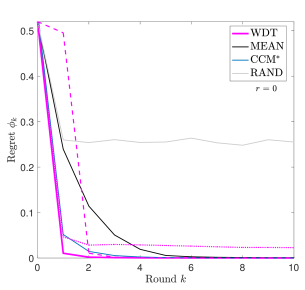
8pt 0.45pt 3pt 0pt

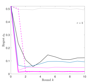
2pt 0.45pt 3pt 0pt

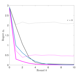
(a) no resignations ($r=0$)

8pt 0.45pt 3pt 0pt

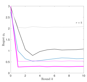
(b) max resignations ($r=b$)

Figure 2: Average regret $\phi_{k}$ versus the round number $k$. The number of job positions is $b=5$ for $n=100$ candidates per round. Score distribution: uniform, $S_{i,k}\sim\mathcal{U}(0,1)$ (top row); exponential, $S_{i,k}\sim\text{Exp}(1),\,\forall i,\,\forall k$ (bottom row). The number of initially empty job positions is $r=0$ (left) and $r=b=5$ (right). Purple lines use WDT in full-information (plain line), partial-information (dashed line) and no-information (dotted line) settings.

V Conclusion and discussion

In this paper we presented a new algorithm, called Warm-starting Dynamic Thresholding (WDT), for the Warm-starting Sequential Selection Problem (WSSP), considering the case where the incoming candidates have scores following a known distribution. The proposed algorithm is based on a dynamic programming approach and achieves optimal threshold estimation at each step of the sequence of interviewed candidates. Experiments have been performed in the multi-round setting, which is interesting for real-world reoccurring recruitment processes. WDT demonstrated a clearly better performance than existing algorithms, regardless the number of initially empty job positions. We additionally proposed a rank-based dynamic programming alternative that can go beyond the need of knowing perfectly the distribution that generates the scores, yet, resulting in satisfying outcomes.

References

- [1] M. Babaioff, N. Immorlica, D. Kempe, and R. Kleinberg, “A knapsack secretary problem with applications,” in APPROX-RANDOM, 2007.
- [2] J. N. Bearden, A. Rapoport, and R. O. Murphy, “Experimental studies of sequential selection and assignment with relative ranks,” in Behavioral Decision Making, vol. 19, 2006, pp. 229–250.
- [3] A. Z. Broder, A. Kirsch, R. Kumar, M. Mitzenmacher, E. Upfal, and S. Vassilvitskii, “The hiring problem and lake Wobegon strategies,” SIAM Journal on Computing, vol. 39, pp. 1223–1255, 2009.
- [4] D. Chisca, M. Lombardi, M. Milano, and B. O’Sullivan, “From offline to online kidney exchange optimization,” IEEE International Conference on Tools with Artificial Intelligence, pp. 587–591, 2018.
- [5] J. Das, F. Py, J. B. Harvey, J. P. Ryan, A. Gellene, R. Graham, D. A. Caron, K. Rajan, and G. S. Sukhatme, “Data-driven robotic sampling for marine ecosystem monitoring,” The International Journal of Robotics Research, vol. 34, no. 12, pp. 1435–1452, 2015.
- [6] M. Fekom, N. Vayatis, and A. Kalogeratos, “The warm-starting sequential selection problem and its multi-round extension,” arXiv preprint, 2019.
- [7] T. S. Ferguson, “Who solved the secretary problem?” in Statistical Science, 1989.
- [8] A. Gnanlet and W. G. Gilland, “Sequential and simultaneous decision making for optimizing health care resource flexibilities,” Decision Sciences, vol. 40, no. 2, pp. 295–326, 2009.
- [9] R. Kleinberg, “A multiple-choice secretary algorithm with applications to online auctions,” in ACM-SIAM Symposium on Discrete Algorithms, 2005, pp. 630–631.
- [10] D. V. Lindley, “Dynamic programming and decision theory,” in Applied Statistics, vol. 101, 1961, pp. 39–51.
- [11] M. L. Nikolaev and G. Y. Sofronov, “A multiple optimal stopping rule for sums of independent random variables,” in Discrete Mathematics and Applications, vol. 17, no. 5, 2007.