Parallel Batch-dynamic Trees via Change Propagation

Abstract

The dynamic trees problem is to maintain a forest subject to edge insertions and deletions while facilitating queries such as connectivity, path weights, and subtree weights. Dynamic trees are a fundamental building block of a large number of graph algorithms. Although traditionally studied in the single-update setting, dynamic algorithms capable of supporting batches of updates are increasingly relevant today due to the emergence of rapidly evolving dynamic datasets. Since processing updates on a single processor is often unrealistic for large batches of updates, designing parallel batch-dynamic algorithms that achieve provably low span is important for many applications.

In this work, we design the first work-efficient parallel batch-dynamic algorithm for dynamic trees that is capable of supporting both path queries and subtree queries, as well as a variety of non-local queries. Previous work-efficient dynamic trees of Tseng et al. were only capable of handling subtree queries under an invertible associative operation [ALENEX’19, (2019), pp. 92–106]. To achieve this, we propose a framework for algorithmically dynamizing static round-synchronous algorithms that allows us to obtain parallel batch-dynamic algorithms with good bounds on their work and span. In our framework, the algorithm designer can apply the technique to any suitably defined static algorithm. We then obtain theoretical guarantees for algorithms in our framework by defining the notion of a computation distance between two executions of the underlying algorithm.

Our dynamic trees algorithm is obtained by applying our dynamization framework to the parallel tree contraction algorithm of Miller and Reif [FOCS’85, (1985), pp. 478–489], and then performing a novel analysis of the computation distance of this algorithm under batch updates. We show that $k$ updates can be performed in $O(k\log(1+n/k))$ work in expectation, which matches the algorithm of Tseng et al. while providing support for a substantially larger number of queries and applications.

1 Introduction

The dynamic trees problem, first posed by Sleator and Tarjan [28] is to maintain a forest of trees subject to the insertion and deletion of edges, also known as links and cuts. Dynamic trees are used as a building block in a multitude of applications, including maximum flows [28], dynamic connectivity and minimum spanning trees [11], and minimum cuts [19], making them a fruitful line of work with a rich history. There are a number of established sequential dynamic tree algorithms, including link-cut trees [28], top trees [29], Euler-tour trees [15], and rake-compress trees [4], all of which achieve $O(\log(n))$ time per operation.

Since they already perform such little work, there is often little to gain by processing single updates in parallel, hence parallel applications typically process batches of updates. We are therefore concerned with the design of parallel batch-dynamic algorithms.

The batch-dynamic setting extends classic dynamic algorithms to accept batches of updates. By applying batches it is often possible to obtain significant parallelism while preserving work efficiency. However, designing and implementing dynamic algorithms for problems is difficult even in the sequential setting, and arguably even more so in the parallel setting.

The goals of this paper are twofold. First and foremost, we are interested in designing a parallel batch-dynamic algorithm for dynamic trees that supports a wide range of applications. On another level, based on the observation that parallel dynamic algorithms are usually quite complex and difficult to design, analyze, and implement, we are also interested in easing the design process of parallel batch-dynamic algorithms as a whole. To this end, we propose a framework for algorithmically dynamizing static parallel algorithms to obtain efficient parallel batch-dynamic algorithms. The framework takes any algorithm implemented in the round synchronous parallel model, and automatically dynamizes it. We then define a cost model that captures the computation distance between two executions of the static algorithm which allows us to bound the runtime of dynamic updates. There are several benefits of using algorithmic dynamization, some more theoretical some practical:

1. Proving correctness of a batch dynamized algorithm relies simply on the correctness of the parallel algorithm, which presumably has already been proven.

2. It is easy to implement different classes of updates. For example, for dynamic trees, in addition to links and cuts, it is very easy to update edge weights or vertex weights for supporting queries such as path length, subtree sums, or weighted diameter. One need only change the values of the weights and propagate.

3. Due to the simplicity of our approach, we believe it is likely to make it easier to program parallel batch-dynamic algorithms, and also result in practical implementations.

Using our algorithmic dynamization framework, we obtain a parallel batch-dynamic algorithm for rake-compress trees that generalizes the sequential data structure work efficiently without loss of generality. Specifically, our main contribution is the following theorem.

Theorem 1.1.

The following operations can be supported on a bounded-degree dynamic tree of size $n$ using the CRCW $\mathsf{PRAM}$: Batch insertions and deletions of $k$ edges in $O(k\log(1+n/k))$ work in expectation and $O(\log(n)\log^{*}(n))$ span w.h.p. Independent parallel connectivity, subtree-sum, path-sum, diameter, lowest common ancestor, center, and median queries in $O(\log n)$ time per query w.h.p.

This algorithm is obtained by dynamizing the parallel tree contraction algorithm of Miller and Reif [21] and performing a novel analysis of the computation distance of the algorithm with respect to any given input.

As some evidence of the general applicability of algorithmic dynamization, in addition to dynamic trees we consider some other applications of the technique. We consider map-reduce based computations in Appendix A, and dynamic sequences with cutting and joining in Appendix B. This leads to another solution to the batch-dynamic sequences problem considered in [30]. We believe the solution here is much simpler, while maintaining the same work bounds. To summarize, the main contributions of this paper are:

1. An algorithmic framework for dynamizing round-synchronous parallel algorithms, and a cost model for analyzing the performance of algorithms resulting from the framework

2. An analysis of the computation distance of Miller and Reif’s tree contraction algorithm under batch edge insertions and deletions in this framework, which shows that it can be efficiently dynamized

3. The first work-efficient parallel algorithm for batch-dynamic trees that supports subtree queries, path queries, and non-local queries such as centers and medians.

Technical overview.

A round-synchronous algorithm consists of a sequence in rounds, where a round executes in parallel across a set of processes, and each process runs a sequencial round computation reading and writing from shared memory and doing local computation. The round synchronous model is similar to Valiant’s well-known Bulk Synchronous Parallel (BSP) model [31], except that communication is done via shared memory.

The algorithmic dynamization works by running the round-synchronous algorithm while tracking all write-read dependences—i.e., a dependence from a write in one round to a read in a later round. Then, whenever a batch of changes are made to the input, a change propagation algorithm propagates the changes through the original computation only rerunning round computations if the values they read have changed. This can be repeated to handle multiple batch changes. We note that depending on the algorithm, changes to the input could drastically change the underlying computation, introducing new dependencies, or invalidating existing ones. Part of the novelty of this paper is bounding both the work and span of this update process.

The idea of change propagation has been applied in the sequential setting and used to generate efficient dynamic algorithms [2, 3]. The general idea of parallel change propagation has also been used in various practical systems [9, 14, 7, 24, 25] but none of them have been analyzed theoretically. To capture the cost of running the change propagation algorithm for a particular parallel algorithm and class of updates we define a computational distance between two computations, which corresponds to the total work of the round computations that differ in the two computations. The input configuration for a computation consists of the input $I$, stored in shared memory, and an initial set of processes $P$. We show the following bounds, where the work is the sum of the time of all round computations, and span is the sum over rounds of the maximum time of any round computation in that round.

Theorem 1.2.

Given a round-synchronous algorithm $A$ that with input configuration $(I,P)$ does $W$ work in $R$ rounds and $S$ span, then

1. the initial run of the algorithm with tracking takes $O(W)$ work in expectation and $O(S+R\log W)$ time w.h.p.,

2. running change propagation from input configuration $(I,P)$ to configuration $(I^{\prime},P^{\prime})$ takes $O(W_{\Delta}+R^{\prime})$ work in expectation and $O(S^{\prime}+R^{\prime}\log W^{\prime})$ time w.h.p., where $W_{\Delta}$ is the computation distance between the two configurations, and $S^{\prime}$,$R^{\prime}$,$W^{\prime}$ are the maximum span, rounds and work for the two configurations,

all on the CRCW $\mathsf{PRAM}$ model.

We show that the work can be reduced to $O(W_{\Delta})$, and that the $\log W$ and $\log W^{\prime}$ terms can be reduced to $\log^{*}W$ when the round-synchronous algorithms have certain restrictions that are satisfied by all of our example algorithms, including our main result on dynamic trees. We also present similar results in other parallel models of computation.

Once we have our dynamization framework and cost model, we use it to develop an algorithm for dynamic trees that support a broad set of queries including subtree sums, path queries, lowest common ancestors, diameter, center, and median queries. This significantly improves over previous work on batch-dynamic Euler tour trees [30], which only support subtree sums, and only when the “summing” function has an inverse (e.g. Euler-tour trees cannot be used to take the maximum over a subtree).

Our batch-dynamic trees algorithm is based on the simple and elegant tree contraction algorithm of Miller and Reif (MR) [22]. Previous work showed that in the sequential setting, this process can be used to generate a rake-compress (RC) tree (or forest), which supports the wide collection of queries mentioned above, all in logarithmic time, w.h.p. [4]. Our approach generalizes this sequential algorithm to allow for batches of edge insertions or deletions, work efficiently in parallel. The challenge is in analyzing the computational distance implied by batch updates in the parallel batch-dynamic setting. In Section 4 we do just that, and obtain the following result:

Theorem 1.3.

In the round synchronous model the MR algorithm does $O(n)$ work in expectation and has $O(\log n)$ rounds and span w.h.p. Furthermore, given forests $T$ with $n$ vertices, and $T^{\prime}$ with $k$ modifications to the edge list of $T$, the computational distance of the round-synchronous MR algorithm on the two inputs is $O(k\log(1+n/k))$ in expectation.

The first sentence follows directly from the original MR analysis. The second is one of the contributions of this paper. The bounds can then be plugged into Theorem 1.2 to show that a set of $k$ edges can be inserted or deleted in a batch in $O(k\log(1+n/k))$ work in expectation and $O(\log^{2}n)$ span w.h.p. The span can be improved to $O(\log n\log^{*}n)$ w.h.p. on the CRCW $\mathsf{PRAM}$ model. The last step in obtaining our dynamic trees framework is to plug the dynamized tree contraction algorithm into the RC trees framework [4] (see Section 5).

Related Work.

In order to better exploit parallelism, work-efficient parallel batch-dynamic algorithms, i.e. algorithms that perform a batch of updates work efficiently and in low span, have gained recent attention and have been developed for several specific problems including computation of Voronoi diagrams [5], incremental connectivity [27], Euler-Tour trees [30], and for fully dynamic connectivity [1]. Parallel batch-dynamic algorithms have also been recently studied in the MPC model [16, 10]. These works show that batch-dynamic algorithms can achieve tight work-efficiency bounds without sacrificing parallelism.

A sequential version of change propagation was initially developed in 2004 [3] and has lead to the development of a sequential dynamic-tree data structure capable of supporting both subtree and path queries [4]. Our results on parallel batch-dynamic trees generalize the sequential results [3, 4] to handle batches of changes work efficiently and in parallel without leading to any loss of generality.

Standalone algorithms for dynamic tree contraction have previously been proposed, but are inefficient and not fully general. In particular, Reif and Tate [26] give an algorithm for parallel dynamic tree contraction that can process a batch of $k$ leaf insertions or deletions in $O(k\log(n))$ work. Unlike our algorithm, theirs is not work efficient, as it performs $\Omega(n\log(n))$ for batches of size $\Omega(n)$, and it can only modify the tree at the leaves.

2 Preliminaries

2.1 Parallel Models

Parallel Random Access Machine ($\bm{\mathsf{PRAM}{}}$). The parallel random access machine ($\mathsf{PRAM}$) model is a classic parallel model with $p$ processors that work in lock-step, connected by a parallel shared-memory [17]. In this paper we primarily consider the Concurrent-Read Concurrent-Write model (CRCW $\mathsf{PRAM}$), where memory locations are allowed to be concurrently read and concurrently written to. If multiple writers write to the same location concurrently, we assume that an arbitrary writer wins. We analyze algorithms on the CRCW $\mathsf{PRAM}$ in terms of their work and span. The span of an algorithm is the minimum running time achievable when arbitrarily many processors are available. The work is the product of the span and the number of processors.

Binary Forking Threaded Random Access Machine ($\bm{$\mathsf{TRAM}${}}$). The threaded random access machine ($\mathsf{TRAM}$) is closely related to the $\mathsf{PRAM}$, but more closely models current machines and programming paradigms. In the binary forking $\mathsf{TRAM}$ (binary forking model for short), a process can fork another process to run in parallel, and can join to wait for all forked calls to complete. In the binary forking model, the work of an algorithm is the total number of instructions it performs, and the span is the longest chain of sequentially dependent instructions. This model can work-efficiently cross-simulate a CRCW $\mathsf{PRAM}$ equipped with the same atomic instructions, and hence all work bounds stated are valid in both. Additionally, an algorithm with $W$ work and $S$ span on the $\mathsf{TRAM}$ can be executed on a $p$ processor $\mathsf{PRAM}$ in time $O(W/p+S)$ [8].

2.2 Parallel Primitives

The following parallel procedures are used throughout the paper. Scan takes as input an array $A$ of length $n$, an associative binary operator $\oplus$, and an identity element $\bot$ such that $\bot\oplus x=x$ for any $x$, and returns the array $(\bot,\bot\oplus A[0],\bot\oplus A[0]\oplus A[1],\ldots,\bot\oplus_{i=0}^{n-2}A[i])$ as well as the overall sum, $\bot\oplus_{i=0}^{n-1}A[i]$. Scan can be done in $O(n)$ work and $O(\log n)$ span (assuming $\oplus$ takes $O(1)$ work) [17] on the CRCW $\mathsf{PRAM}$, $O(\log(n))$ span in the binary forking model.

Filter takes an array $A$ and a predicate $f$ and returns a new array containing $a\in A$ for which $f(a)$ is true, in the same order as in $A$. Filter can both be done in $O(n)$ work and $O(\log n)$ span on the CRCW $\mathsf{PRAM}$ (assuming $f$ takes $O(1)$ work) [17], $O(\log(n))$ span in the binary forking model. The Approximate Compaction problem is similar to a Filter. It takes an array $A$ and a predicate $f$ and returns a new array containing $a\in A$ for which $f(a)$ is true where some of the entries in the returned array can have a null value. The total size of the returned array is at most a constant factor larger than the number of non-null elements. Gil et al. [12] describe a parallel approximate compaction algorithm that uses linear space and achieves $O(n)$ work and $O(\log^{*}(n))$ span w.h.p. on the CRCW $\mathsf{PRAM}$.

A semisort takes an input array of elements, where each element has an associated key and reorders the elements so that elements with equal keys are contiguous, but elements with different keys are not necessarily ordered. The purpose is to collect equal keys together, rather than sort them. Semisorting a sequence of length $n$ can be performed in $O(n)$ expected work and $O(\log n)$ depth w.h.p. on the CRCW $\mathsf{PRAM}$ and in the binary forking model assuming access to a uniformly random hash function mapping keys to integers in the range $[1,n^{O(1)}]$ [13].

3 Dynamization Framework

3.1 Round-synchronous algorithms

In this framework, we consider dynamizing algorithms that are round synchronous. The round synchronous framework encompasses a range of classic BSP [31] and $\mathsf{PRAM}$ algorithms. A round-synchronous algorithm consists of $M$ processes, with process IDs bounded by $O(M)$. The algorithm performs sequential rounds in which each active process executes, in parallel, a round computation. At the end of a round, any processes can decide to retire, in which case they will no longer execute in any future round. The algorithm terminates once there are no remaining active processes—i.e., they have all retired. Given a fixed input, round-synchronous algorithms must perform deterministically. Note that this does not preclude us from implementing randomized algorithms (indeed, our dynamic trees algorithm is randomized), it just requires that we provide the source of randomness as an input to the algorithm, so that its behavior is identical if re-executed. An algorithm in the round synchronous framework is defined in terms of a procedure ComputeRound$(r,p)$, which performs the computation of process $p$ in round $r$. The initial run of a round-synchronous algorithm must specify the set $P$ of initial process IDs.

Memory model. Processes in a round-synchronous algorithm may read and write to local memory that is not persisted across rounds. They also have access to a shared memory. The input to a round-synchronous is the initial contents of the shared memory. Round computations can read and write to shared memory with the condition that writes do not become visible until the end of the round. We require that reads only access shared locations that have been written to, and that locations are only written to once, hence concurrent writes are not permitted. The contents of the shared memory at termination of an algorithm is considered to be the algorithm’s output. Change propagation is driven by tracking all reads and writes to shared memory.

Pseudocode. We describe round-synchronous algorithms using the following primitives:

1. The read instruction reads the given shared memory locations and returns their values,

2. The write instruction writes the given value to the given shared memory location.

3. Processes may retire by invoking the retire process instruction.

Measures. The following measures will help us to analyse the efficiency of round-synchronous algorithms. For convenience, we define the input configuration of a round-synchronous algorithm as the pair $(I,P)$, where $I$ is the input to the algorithm (i.e. the initial state of shared memory) and $P$ is the set of initial process IDs.

Definition 3.1 (Initial work, Round complexity, and Span).

The initial work of a round-synchronous algorithm on some input configuration $(I,P)$ is the sum of the work performed by all of the computations of each processes over all rounds when given that input. Its round complexity is the number of rounds that it performs, and its span is the sum of the maximum costs per round of the computations performed by each process.

3.2 Change propagation

Given a round-synchronous algorithm, a dynamic update consists of a change to the input configuration, i.e. changing some of the input values in shared memory, and optionally, adding or deleting processes. The initial run and change propagation algorithms maintain the following data:

1. $R_{r,p}$, the memory locations read by process $p$ in round $r$

2. $W_{r,p}$, the memory locations written by process $p$ in round $r$

3. $S_{m}$, the set of round, process pairs that read memory location $m$

4. $X_{r,p}$, which is true if process $p$ retired in round $r$

Algorithm 1 depicts the procedure for executing the initial run of a round-synchronous algorithm before making any dynamic updates.

Algorithm 1 Initial run

1:procedure Run($P$)

2:   local $r\leftarrow 0$

3:   while $P\neq\emptyset$ do

4:     for each process $p\in P$ do in parallel

5:       ComputeRound($r,p$)

6:        $R_{r,p}$ $\leftarrow$ $\{$memory locations read by $p$ in round $r\}$

7:        $W_{r,p}$ $\leftarrow$ $\{$memory locations written to by $p$ in round $r\}$

8:        $X_{r,p}\leftarrow$ (true if $p$ retired in round $r$ else false)      

9:     for each $m\in\cup_{p\in P}R_{r,p}$ do in parallel

10:        $S_{m}$ $\leftarrow$ $S_{m}\cup\{(r,p)\ |\ m\in R_{r,p}\land\ p\in P\}$      

11:      $P\leftarrow P\setminus\{p\in P:X_{r,p}=\textbf{true}\}$

12:     $r\leftarrow r+1$    

To help formalize change propagation, we define the notion of an affected computation. The task of change propagation is to identify the affected computations and rerun them.

Definition 3.2 (Affected computation).

Given a round-synchronous algorithm $A$ and two input configurations $(I,P)$ and $(I^{\prime},P^{\prime})$, the affected computations are the round and process pairs $(r,p)$ such that either:

1. process $p$ runs in round $r$ on one input configuration but not the other

2. process $p$ runs in round $r$ on both input configurations, but reads a variable from shared memory that has a different value in one configuration than the other

The change propagation algorithm is depicted in Algorithm 2.

Algorithm 2 Change propagation

1:// $U$ = sequence of memory locations that have been modified

2:// $P^{+}$ = sequence of new process IDs to create

3:// $P^{-}$ = sequence of process IDs to remove

4:procedure Propagate($U$, $P^{+}$, $P^{-}$)

5:   local $D\leftarrow P^{-}$ // Processes that died earlier than before

6:   local $L\leftarrow P^{+}$ // Processes that lived longer than before

7:   local $A$ $\leftarrow$ $\emptyset$ // Affected computations at each round

8:   local $r\leftarrow 0$

9:   while $U\neq\emptyset\lor D\neq\emptyset\lor L\neq\emptyset\lor\exists r^{\prime}\geq r:\ (A_{r^{\prime}}\neq\emptyset)$ do

10:     // Determine the computations that become affected

11:     // due to the newly updated memory locations $U$

12:      $\textbf{local }{}A^{\prime}\leftarrow{}\cup_{m\in U}S_{m}$

13:     for each $r^{\prime}\in\cup_{(r^{\prime},p)\in A^{\prime}}\{r^{\prime}\}$ do in parallel

14:        $A_{r^{\prime}}\leftarrow{}A_{r^{\prime}}\cup\{p\ |\ (r^{\prime},p)\in A^{\prime}\}$      

15:      local $P$ $\leftarrow$ $A_{r}\setminus D$ // Processes to rerun

16:     // Forget the prior reads of all processes that are

17:     // now dead or will be rerun on this round

18:     for each $m\in\cup_{p\in P\cup D}R_{r,p}$ do in parallel

19:        $S_{m}$ $\leftarrow$ $S_{m}\setminus\{(r,p)\ |\ m\in R_{r,p}\land\ p\in P\cup D\}$      

20:      local $X^{\text{prev}}=\{p\mapsto X_{r,p}\ |\ p\in P\}$

21:     // (Re)run all changed or newly live processes

22:     for each process $p$ in $P\cup L$ do in parallel

23:        ComputeRound($r,p$)

24:       $R_{r,p}$ $\leftarrow$ $\{$memory locations read by $p$ in round $r\}$

25:       $W_{r,p}$ $\leftarrow$ $\{$memory locations written to by $p$ in round $r\}$

26:        $X_{r,p}\leftarrow$ (true if $p$ retired in round $r$ else false)      

27:     // Remember the reads performed by processes on this round

28:     for each $m\in\cup_{p\in P\cup L}R_{r,p}$ do in parallel

29:        $S_{m}$ $\leftarrow$ $S_{m}\cup\{(r,p)\ |\ m\in R_{r,p}\land\ p\in P\cup L\}$      

30:     // Update the sets of changed memory locations,

31:     // newly live processes, and newly dead processes

32:      $U\leftarrow\cup_{p\in(P\cup L)}W_{r,p}$

33:      $L^{\prime}\leftarrow\{p\in P\ |\ X^{\text{prev}}_{p}=\textbf{true}\land X_{r,p}=\textbf{false}\}$

34:     $L\leftarrow L\ \cup L^{\prime}\setminus\{p\in L\ |\ X_{r,p}=\textbf{true}\}$

35:     $D^{\prime}\leftarrow\{p\in P\ |\ X^{\text{prev}}_{p}=\textbf{false}\land X_{r,p}=\textbf{true}\}$

36:      $D\leftarrow D\cup D^{\prime}\setminus\{p\in D\ |\ X_{r,p}=\textbf{true}\}$

37:     $r\leftarrow r+1$    

Algorithm 2 works by maintaining the affected computations as three disjoint sets, $P$, the set of processes that read a memory location that was rewritten, $L$, processes that outlived their previous self, i.e. that retired the last time they ran, but did not retire when re-executed, and $D$, processes that retired earlier than their previous self. First, at each round, the algorithm determines the set of computations that should become affected because of shared memory locations that were rewritten in the previous round (Lines 12–14). These are used to determine $P$, the set of affected computations to rerun this round (Line 15). To ensure correctness, the algorithm must then reset the reads that were performed by the computations that are no longer alive, or that will be reran, since the set of locations that they read may differ from last time (Lines 18–19). Lines 22–26 perform the re-execution of all processes that read a changed memory location, or that lived longer (did not retire) than in the previous configuration. The algorithm then subscribes the reads of these computations to the memory locations that they read (Lines 28–29). Finally, on Lines 32–36, the algorithm updates the set of changed memory locations ($U$), the set of computations that lived longer than their previous self ($L$) and the set of computations that retired earlier then their previous self ($D$).

3.3 Correctness

In this section, we sketch a proof of correctness of the change propagation algorithm (Algorithm 2). Intuitively, correctness is assured because of the write-once condition on global shared memory, which ensures that computations can not have their output overwritten, and hence do not need to be re-executed unless data that they depend on is modified.

Lemma 3.1.

Given a dynamic update, re-executing only the affected computations for each round will result in the same output as re-executing all computations on the new input.

Proof.

Since by definition they read the same values, computations that are not affected, if re-executed, would produce the same output as they did the first time. Since all shared memory locations can only be written to once, values written by processes that are not re-executed can not have been overwritten, and hence it is safe to not re-execute them, as their output is preserved. Therefore re-executing only the affected computations will produce the same output as re-executing all computations. ∎

Theorem 3.1 (Consistency).

Given a dynamic update, change propagation correctly updates the output of the algorithm.

Proof sketch.

Follows from Lemma 3.1 and the fact that all reads and writes to global shared memory are tracked in Algorithm 2, and since global shared memory is the only method by which processes communicate, all affected computations are identified. ∎

3.4 Cost analysis

To analyze the work of change propagation, we need to formalize a notion of computation distance. Intuitively, the computation distance between two computations is the work performed by one and not the other. We then show that change propagation can efficiently re-execute the affected computations in work proportional to the computation distance.

Definition 3.3 (Computation distance).

Given a round-synchronous algorithm $A$ and two input configurations, the computation distance $W_{\Delta}$ between them is the sum of the work performed by all of the affected computations with respect to both input configurations.

Theorem 3.2.

Given a round-synchronous algorithm $A$ with input configuration $(I,P)$ that does $W$ work in $R$ rounds and $S$ span, then

1. the initial run of the algorithm with tracking takes $O(W)$ work in expectation and $O(S+R\cdot\log(W))$ span w.h.p.,

2. running change propagation on a dynamic update to the input configuration $(I^{\prime},P^{\prime})$ takes $O(W_{\Delta}+R^{\prime})$ work in expectation and $O(S^{\prime}+R^{\prime}\log(W^{\prime}))$ span w.h.p., where $S^{\prime},R^{\prime},W^{\prime}$ are the maximum span, rounds, and work of the algorithm on the two input configurations,

These bounds hold on the CRCW $\mathsf{PRAM}$ and in the binary forking $\mathsf{TRAM}$ model.

Proof.

We begin by analyzing the initial run. By definition, all executions of the round computations, ComputeRound, take $O(W)$ work and $O(S)$ span in total, with at most an additional $O(\log(n))=O(\log(W))$ span to perform the parallel for loop. We will show that all additional work can be charged to the round computations, and that at most an additional $O(\log(W))$ span overhead is incurred.

We observe that $R_{r,p},W_{r,p}$ and $X_{r,p}$ are at most the size of the work performed by the corresponding computations, hence the cost of Lines 6 – 8 can be charged to the computation. The reader sets $S_{m}$ can be implemented as dynamic arrays with lazy deletion (this will be discussed during change propagation). To append new elements to $S_{m}$ (Line 10), we can use a semisort performing linear work in expectation to first bucket the shared memory locations in $\cup_{p\in P}R_{r,p}$, whose work can be charged to the corresponding computations that performed the reads. This adds an additional $O(\log(W))$ span w.h.p. since the number of reads is no more than $W$ in total. Finally, removing retired computations from $P$ (Line 11 requires a compaction operation. Since compaction takes linear work, it can be charged to the execution of the corresponding processes. The span of compaction is at most $O(\log(W))$ in all models.

Summing up the above, we showed that all additional work can be charged to the round computations, and the algorithm incurs at most $O(\log(W))$ additional span per round w.h.p. Hence the cost of the initial run is $O(W)$ work in expectation and $O(S+R\cdot\log(W))$ span w.h.p.

We now analyze the change propagation procedure (Algorithm 2). The core of the work is the re-execution of the affected readers on Line 23, which, by definition takes $O(W_{\Delta})$ work, and $O(S^{\prime})$ span, with at most $O(\log(W^{\prime}))$ additional span to perform the parallel for loop. Since some rounds may have no affected computations, the algorithm could perform up to $O(R^{\prime})$ additional work to process these rounds. We will show that all additional work can be charged to the affected computations, and that no operation incurs more than an additional $O(\log(W^{\prime}))$ span.

Lines 12 – 14 bucket the newly affected computations by round. This can be achieved with an expected linear work semisort and by maintaining the $A_{r}$ sets as dynamic arrays. The work is chargeable to the affected computations and the span is at most $O(\log(W^{\prime}))$ w.h.p. Computing the current set of affected computations (Line 15) requires a filter/compaction operation, whose work is charged to the affected computations and span is at most $O(\log(W^{\prime}))$.

Updating the reader sets $S_{m}$ (Line 19) can be done as follows. We maintain $S_{m}$ as dynamic arrays with lazy deletion, meaning that we delete by marking the corresponding slot as empty. When more than half of the slots have been marked empty, we perform compaction, whose work is charged to the updates and whose span is at most $O(\log(W^{\prime}))$. In order to perform deletions in constant time, we augment the set $R_{r,p}$ so that it remembers, for each entry $m$, the location of $(r,p)$ in $S_{m}$. Therefore these updates take constant amortized work each (using a dynamic array), charged to the corresponding affected computations, and at most $O(\log(W^{\prime}))$ span if a resize/compaction is triggered.

$X^{\text{prev}}$ can be implemented as an array of size $|P|$, with work charged to the affected computations in $P$. As in the initial run, the cost of updating $R_{r,p},W_{r,p}$ and $X_{r,p}$ can also be charged to the work performed by the affected computations.

Updating the reader sets $S_{m}$ (Line 29) is a matter of appending to dynamic arrays, and, as mentioned earlier, remembering for each $m\in R_{r,p}$ $m$, the location of $(r,p)$ in $S_{m}$. The work performed can be charged to the affected computations, and the additional span is at most $O(\log(W^{\prime}))$.

Collecting the updated locations $U$ (Line 32) can similarly be charged to the affected computations, and incurs no more than $O(\log(W^{\prime}))$ span. On Lines 33 – 36, the sets $L^{\prime}$ and $D^{\prime}$ are computed by a compaction over $P$, whose work is charged to the affected computations in $P$. Updating $L$ and $D$ correspondingly requires a compaction operation, whose work is charged to the affected computations in $L$ and $D$ respectively. Each of these compactions costs $O(\log(W^{\prime}))$ span.

We can finally conclude that all additional work performed by change propagation can be charged to the affected computations, and hence to the computation distance $W_{\Delta}$, while incurring at most $O(\log(W^{\prime}))$ additional span per round w.h.p. Therefore the total work performed by change propagation is $O(W_{\Delta}+R^{\prime})$ in expectation and the span is $O(S^{\prime}+R^{\prime}\cdot\log(W^{\prime}))$ w.h.p. ∎

We now show that for a special class of round-synchronous algorithms, the span overhead can be reduced. Our dynamic trees algorithm and our other examples all fall into this special case.

Definition 3.4.

A restricted round-synchronous algorithm is a round-synchronous algorithm such that each round computation performs only a constant number of reads and writes, and each shared memory location is read only by a constant number of computations, and only in the round directly after it was written.

Theorem 3.3.

Given a restricted round-synchronous algorithm $A$ with input configuration $(I,P)$ that does $W$ work in $R$ rounds and $S$ span, then

1. the initial run of the algorithm with tracking takes $O(W)$ work and $O(S+R\cdot\mathcal{C}{}(W))$ span,

2. running change propagation on a dynamic update to the input configuration $(I^{\prime},P^{\prime})$ takes $O(W_{\Delta})$ work and $O(D^{\prime}+R^{\prime}\mathcal{C}{}(W^{\prime}))$ span, where $D^{\prime},R^{\prime},W^{\prime}$ are the maximum span, rounds, and work of the algorithm on the two input configurations,

where $\mathcal{C}{}(W)$ is the cost of compaction, which is at most

1. $O(\log^{*}(W))$ w.h.p. on the CRCW $\mathsf{PRAM}$,

2. $O(\log(W))$ on the binary forking $\mathsf{TRAM}$.

Furthermore, the work bounds are only randomized (in expectation) on the CRCW $\mathsf{PRAM}$.

Proof sketch.

Rather than recreate the entirety of the proof of Theorem 3.2, we will simply sketch the differences. In essence, we obtain the result by removing the uses of scans, and semisorts, which were the main cause of the $O(\log(W^{\prime}))$ span overhead and the randomized work. Instead, we rely only on (possibly approximate) compaction, which is only randomized on the CRCW $\mathsf{PRAM}$, and takes $O(\mathcal{C}{}(W^{\prime}))$ span. We also lose the $R^{\prime}$ term in the work since computations can only read from locations written in the previous round, and hence the set of rounds on which there exists an affected computation must be contiguous.

The main technique that we will make use of is the sparse array plus compaction technique. In situations where we wish to collect a set of items from each executed process, we would, in the unrestricted model, require a scan, which costs $O(\log(W^{\prime}))$ span on the CRCW $\mathsf{PRAM}$. If each executed process, however, only produces a constant number of these items, we can allocate an array that is a constant size larger than the number of processes, and each process can write its set of items to a designated offset. We can then perform (possibly approximate) compaction on this array to obtain the desired set, with at most a constant factor additional blank entries. This takes $O(\mathcal{C}{}(W^{\prime}))$ span.

Maintaining $S_{m}$ in the initial run and during change propagation is the first bottleneck, originally requiring a semisort. Since each computation performs a constant number of writes, we can collect the writes using the sparse array plus compaction technique. Since, in the restricted model, each modifiable will only be read by a constant number of readers, we can update $S_{m}$ in constant time.

To compute the affected computations $A_{r}$ also originally required a semisort, but in the restricted model, since all reads happen on the round directly after the write, no semisort is needed, since they will all have the same value of $r$. Collecting the affected computations from the written modifiables can also be achieved using the sparse array and compaction technique, using the fact that each computation wrote to a constant number of modifiables, and each modifiable is subsequently read by a constant number of computations. Additionally, $A_{r}$ will be empty at the beginning of round $r$, so computing $P$ requires only a compaction operation.

Lastly, collecting the updated locations $U$ can also be performed using the sparse array and compaction technique. In summary, we can replace all originally $O(\log(W^{\prime}))$ span operations with $O(\mathcal{C}{}(W^{\prime}))$ equivalents in the restricted setting, and hence we obtain a span bound of $O(S^{\prime}+R^{\prime}\cdot\mathcal{C}{}(W^{\prime}))$ for both the initial run and change propagation. ∎

Remark 3.1 (Space usage).

We do not formally specify an implementation of the memory model, but one simple way to achieve good space bounds is to use hashtables to implement global shared memory. Each write to a particular global shared memory location maps to an entry in the hashtable. When a round computation is invalidated during a dynamic update, its writes can be purged from the hashtable to free up space, preventing unbounded space blow up. Since the algorithm must also track the reads of each global shared memory location, using this implementation, the space usage is proportional to the number of shared memory reads and writes. In the restricted round-synchronous model, the number of reads must be proportional to the number of writes, and hence the space usage is optimal, since any strategy for storing shared memory must use at least this much.

4 Dynamizing Tree Contraction

In this section, we show how to obtain a dynamic tree contraction algorithm by applying our automatic dynamization technique to the static tree contraction algorithm of Miller and Reif [21]. We will then, in Section 5, describe how to use this to obtain a powerful parallel batch-dynamic trees framework.

Tree contraction. Tree contraction is the process of shrinking a tree down to a single vertex by repeatedly performing local contractions. Each local contraction deletes a vertex and merges its adjacent edges if it had degree two. Tree contraction has a number of useful applications, studied extensively in [22, 23, 4]. It can be used to perform various computations by associating data with edges and vertices and defining how data is accumulated during local contractions.

Various versions of tree contraction have been proposed depending on the specifics of local contractions. We consider an undirected variant of the randomized version proposed by Miller and Reif [21], which makes use of two operations: rake and compress. The former removes all nodes of degree one from the tree, except in the case of a pair of adjacent degree one vertices, in which case only one of them is removed by tiebreaking on the vertex IDs. The latter operation, compress, removes an independent set of vertices of degree two that are not adjacent to any vertex of degree one. Compressions are randomized with coin flips to break symmetry. Miller and Reif showed that it takes $O(\log n)$ rounds w.h.p. to fully contract a tree of $n$ vertices in this manner.

Input forests. The algorithms described here operate on undirected forests $F=(V,E)$, where $V$ is a set of vertices, and $E$ is a set of undirected edges. If $(u,v)\in E$, we say that $u$ and $v$ are adjacent, or that they are neighbors. A vertex with no neighbors is said to be isolated, and a vertex with one neighbour is called a leaf.

We assume that the forests given as input have bounded degree. That is, there exists some constant $t$ such that each vertex has at most $t$ neighbors. We will explain how to handle arbitrary-degree trees momentarily.

The static algorithm. The static tree contraction algorithm (Algorithm 3) works in rounds, each of which takes a forest from the previous round as input and produces a new forest for the next round. On each round, some vertices may be deleted, in which case they are removed from the forest and are not present in all remaining rounds. Let $F^{i}=(V^{i},E^{i})$ be the forest after $i$ rounds of contraction, and thus $F^{0}=F$ is the input forest. We say that a vertex $v$ is alive at round $i$ if $v\in V^{i}$, and is dead at round $i$ if $v\not\in V^{i}$. If $v\in V^{i}$ but $v\not\in V^{i+1}$ then $v$ was deleted in round $i$. There are three ways for a vertex to be deleted: it either finalizes, rakes, or compresses. Finalization removes isolated vertices. Rake removes all leaves from the tree, with one special exception. If two leaves are adjacent, then to break symmetry and ensure that only one of them rakes, the one with the lower identifier rakes into the other. Finally, compression removes an independent set of degree two vertices that are not adjacent to any degree one vertices, as in Miller and Reif’s algorithm. The choice of which vertices are deleted in each round is made locally for each vertex based upon its own degree, the degrees of its neighbors, and coin flips for itself and its neighbors. As in the list contraction, for coin flips, we assume a function $\textsc{Heads}(i,v)$ which indicates whether or not vertex $v$ flipped heaps on round $i$. It is important that $\textsc{Heads}(i,v)$ is a function of both the vertex and the round number, as coin flips must be repeatable for change propagation to be correct.

The algorithm produces a contraction data structure which serves as a record of the contraction process. The contraction data structure is a tuple, $(A,D)$, where $A[i][u]$ is a list of pairs containing the vertices adjacent to $u$ in round $i$, and the positions of $u$ in the adjacency lists of the adjacent vertices. $D[u]$ stores the round on which vertex $u$ contracted. The algorithm also records leaf$[i][u]$, which is true if vertex $u$ is a leaf at round $i$.

Updates. We consider update operations that implement the interface of a batch-dynamic tree data structure. This requires supporting batches of links and cuts. A link (insertion) connects two trees in the forest by a newly inserted edge. A cut (deletion) deletes an edge from the forest, separating a single tree into two trees. We formally specify the interface for batch-dynamic trees and give a sample implementation of their operations in terms of the tree contraction data structure in Appendix C.

Handling trees of arbitrary degree. To handle trees of arbitrary degree, we can split each vertex into a path of vertices, one for each of its neighbors. This technique is standard and has been described in [18], for example. This results in an underlying tree of degree $3$, with at most $O(n+m)$ vertices and $O(m)$ edges for an initial tree of $n$ vertices and $m$ edges. For edge-weighted trees, the additional edges can be given a suitable identity or null weight to ensure that query values remain correct. It is simple to maintain such a transformation dynamically. When performing a batch insertion, a work-efficient semisort can be used to group each new neighbour by their endpoints, and then for each vertex, an appropriate number of new vertices can be added to the path. Batch deletion can be handled similarly.

4.1 Algorithm

An implementation of the tree contraction algorithm in our framework is shown in Algorithm 3.

Algorithm 3 Tree contraction algorithm

1:procedure ComputeRound($i,u$)

2:   local $((v_{1},p_{1}),...,(v_{t},p_{t}))$, $\ell$ $\leftarrow$ read($A[i][u]$, leaf$[i][u]$)

3:   if $v_{i}=\perp\forall i$ then

4:     DoFinalize($i,u$)

5:   else if $\ell$ then

6:     local $(v,p)$ $\leftarrow$ $(v_{i},p_{i})$ such that $v_{i}\neq\perp{}$

7:     local $\ell^{\prime}$ $\leftarrow$ read(leaf$[i][v]$)

8:     if $\lnot\ell^{\prime}\lor\ u<v$ then DoRake($i,u,(v,p)$)

9:     else DoAlive($i,u,((v_{1},p_{1}),...,(v_{t},p_{t}))$)      

10:   else

11:     if $\exists(v,p),(v^{\prime},p^{\prime}):\{v_{1},...,v_{t}\}\setminus\{\perp\}=\{v,v^{\prime}\}$ then

12:       local $\ell^{\prime},\ell^{\prime\prime}$ $\leftarrow$ read(leaf$[i][v]$, leaf$[i][v^{\prime}]$)

13:       local $c$ $\leftarrow$ $\textsc{Heads}(i,u)\ \land\ \lnot\textsc{Heads}(i,v)\ \land\ \lnot\textsc{Heads}(i,v^{\prime})$

14:       if ($\lnot\ell^{\prime}\land\ \lnot\ell^{\prime\prime}\land\ c$) then

15:         DoCompress($i,u,(v,p),(v^{\prime},p^{\prime})$)

16:       else 

17:         DoAlive($i,u,((v_{1},p_{1}),...,(v_{t},p_{t}))$)        

18:     else

19:       DoAlive($i,u,((v_{1},p_{1}),...,(v_{t},p_{t}))$)         

20:

21:procedure DoRake($i,u,(v,p)$)

22:   write($A[i+1][v][p]$, $\perp$)

23:   write($D[u]$, $i$)

24:   retire process

25:

26:procedure DoFinalize($i,u$)

27:   write($D[u]$, $i$)

28:   retire process

29:

30:procedure DoCompress($i,u,(v,p),(v^{\prime},p^{\prime})$)

31:   write($A[i+1][v][p]$, $(v^{\prime},p^{\prime})$)

32:   write($A[i+1][v^{\prime}][p^{\prime}]$, $(v,p)$)

33:   retire process

34:

35:procedure DoAlive($i,u,((v_{1},p_{1}),...,(v_{t},p_{t}))$)

36:   local nonleaves $\leftarrow$ $0$

37:   for $j\leftarrow 1\ \textbf{to }t$ do

38:     if $v_{j}\neq\perp$ then

39:       write($A[i+1][v_{j}][p_{j}]$, $(u,j)$)

40:       nonleaves += 1 - read(leaf$[i][v_{j}]$)

41:     else 

42:       write($A[i+1][u][j]$, $\perp$)         

43:   write(leaf$[i+1][u]$, nonleaves $=1$)

4.2 Analysis

We analyse the initial work, round, complexity, span, and computation distance of the tree contraction algorithm to obtain bounds for building and updating a parallel batch-dynamic trees data structure. Proofs are given in Appendix D.

Theorem 4.1.

Given a forest of $n$ vertices, the initial work of tree contraction is $O(n)$ in expectation, the round complexity and the span is $O(\log(n))$ w.h.p. and the computation distance induced by updating $k$ edges is $O(k\log(1+n/k))$ in expectation.

5 Parallel Rake-compress Trees

Dynamic trees typically provide support for dynamic connectivity queries. Most dynamic tree data structures also support some form of augmented value query. For example, Link-cut trees [28] support root-to-vertex path queries, and Euler-tour trees [15] support subtree sum queries. Top trees [29, 6] support both path and subtree queries, as well as non-local queries such as centers and medians, but are not amenable to parallelism. The only existing parallel batch-dynamic tree data structure is that of Tseng et al. [30], which is based on Euler-tour trees, and hence only handles subtree queries, and only when the associative operation is invertible.

Rake-compress trees [4] (RC trees) are another sequential dynamic trees data structure, based on tree contraction, and have also been shown to be capable of handling both path and subtree queries, as well as non-local queries, all in $O(\log(n))$ time. In this section, we will explain how our parallel batch-dynamic algorithm for tree contraction can be used to derive a parallel batch-dynamic version of RC trees, leading to the first work-efficient algorithm for batch-dynamic trees that can handle this wide range of queries. We use a slightly different set of definitions than the original presentation of RC trees in [4], which correct some subtle corner cases and simplify the exposition, although the resulting data structure is the same, and hence all of the query algorithms for sequential RC trees work on our parallel version.

Contraction and clusters. RC trees are based on the idea that the tree contraction process can be interpreted as a recursive clustering of the original tree. Formally, a cluster is a connected subset of vertices and edges of the original tree. Note, importantly, that a cluster may contain an edge without containing both of its endpoints. The boundary vertices of a cluster $C$ are the vertices $v\notin C$ that are adjacent to an edge $e\in C$. The degree of a cluster is the number of boundary vertices of that cluster. The vertices and edges of the original tree form the base clusters. Clusters are merged using the following simple rule: Whenever a vertex $v$ is deleted, all of the clusters that have $v$ as a boundary vertex are merged with the base cluster containing $v$. We can therefore see that all clusters formed will have degree at most two. A cluster of degree zero is called a nullary cluster, a cluster of degree one a unary cluster, and a cluster of degree two a binary cluster. All non-base clusters have a unique representative vertex, which corresponds to the vertex that was deleted to form it. For additional clarity, we provide figures in Appendix E that explain what each kind of formed cluster looks like in more detail.

5.1 Building and maintaining RC trees

Given a tree and an execution of the tree contraction algorithm, the RC tree consists of nodes which correspond to the clusters formed by the contraction process. The children of a node are the nodes corresponding to the clusters that merged together to form it. An example tree, a clustering, and the corresponding RC tree are depicted in Figure 1. Note that in the case of a disconnected forest, the RC tree will have multiple roots.

We will sketch here how to maintain an RC tree subject to batch-dynamic updates in parallel using our algorithm for parallel batch-dynamic tree contraction. This requires just two simple augmentations to the tree contraction algorithm. Recall that tree contraction (Algorithm 3) maintains an adjacency list for each vertex at each round. Whenever a neighbour $u$ of a vertex $v$ rakes into $v$, the process $u$ writes a null value into the corresponding position in $v$’s adjacency list. This process can be augmented to also write, in addition to the null value, the identity of the vertex that just raked. We make one additional augmentation. When storing the data for a neighboring edge in a vertex’s adjacency list, we additionally write the name of the representative vertex if that edge corresponds to a compression, or null if the edge is an edge of the original tree. The RC tree can then be inferred using this augmented data as follows.

1. Given any cluster $C$ with representative $v$, its unary children can be determined by looking at the vertices that raked into $v$. The children are precisely the unary clusters represented by these vertices. For the final cluster, these are its only children.

2. Given a binary or unary cluster $C$ with representative $v$, its binary children can be determined by inspecting $v$’s adjacency list at the moment it was deleted. The binary clusters corresponding to the edges adjacent to $v$ at its time of death are the binary children of the cluster $C$.

It then suffices to observe that this information about the clusters can be recorded during the contraction process. By employing change propagation, the RC tree can therefore be maintained subject to batch-dynamic updates. Since each cluster consists of a constant amount of information, this can be done in the same work and span bounds as the tree contraction algorithm. We therefore have the following result.

Theorem 5.1.

We can maintain a rake-compress tree of a tree on $n$ vertices subject to batch insertions and batch deletions of size $k$ in $O(k\log(1+n/k))$ work in expectation and $O(\log^{2}(n))$ span per update w.h.p. The span can be improved to $O(\log(n)\log^{*}(n))$ w.h.p. on the CRCW $\mathsf{PRAM}$.

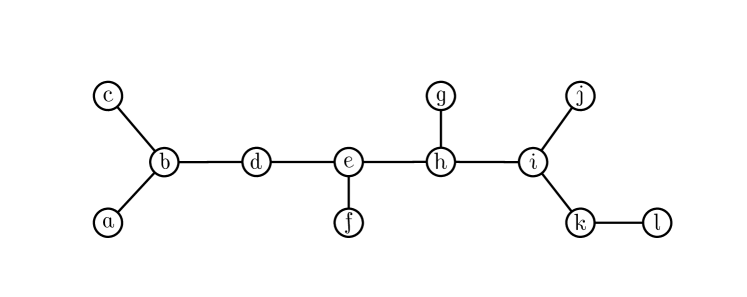
(a) A tree

(b) A recursive clustering of the tree produced by tree contraction. Clusters produced in earlier rounds are depicted in a darker color.

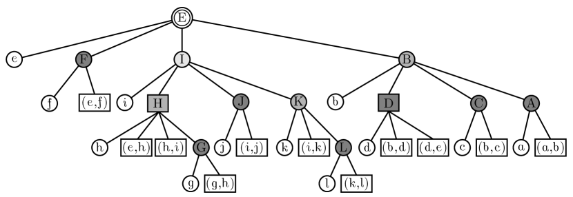
(c) The corresponding RC tree. (Non-base) unary clusters are shown as circles, binary clusters as rectangles, and the finalize (nullary) cluster at the root with two concentric circles. The base clusters (the leaves) are labeled in lowercase, and the composite clusters are labeled with the uppercase of their representative.

Figure 1: A tree, a clustering, and the corresponding RC tree.

5.2 Applications

Most kinds of queries assume that the vertices and/or edges of the input tree are annotated with data, such as weights or labels. In order to support queries, each cluster is annotated with some additional information. The algorithm must then specify how to combine the data from multiple constituent clusters whenever a set of clusters merge. These annotations are generated during the tree contraction algorithm, and are therefore available for querying immediately after performing an update.

Once the clusters are annotated with the necessary data, the queries themselves typically perform a bottom-up or top-down traversal of the RC tree, or possibly in the case of more complicated queries, a combination of both. A variety of application queries is described in [4].

Batch queries. For some applications, we can also implement batch queries, in which we answer $k$ queries simultaneously in $O(k\log(1+n/k))$ work in expectation and $O(\log(n))$ span w.h.p. This improves upon the work bound of $O(k\log(n))$ obtained by simply running the queries in parallel naively. The general idea is to detect when multiple bottom-up traversals would intersect, and to have only one of them proceed up the RC tree. Upon reaching the root, the computation can backtrack down the tree in parallel and distribute the answers to the query. The most obvious query for which this technique is applicable is finding a representative vertex of the connected component containing a vertex. When traversing upwards, if multiple query paths intersect, then only one proceeds up the tree and brings the answer back down for the other ones. The following theorem formalizes the advantage of performing batch queries. The proof appears in Appendix E.2

Theorem 5.2.

Given a tree on $n$ vertices and a corresponding $RC$ tree, $k$ root-to-leaf paths in the RC tree touch $O(k\log(1+n/k))$ distinct RC tree nodes in expectation.

6 Conclusion

In this paper we showed that we can obtain work-efficient parallel batch-dynamic algorithms by applying an algorithmic dynamization technique to corresponding static algorithms. Using this technique, we obtained the first work-efficient parallel algorithm for batch-dynamic trees that supports more than just subtree queries. It can handle path queries and non-local queries such as centers and medians. Our framework also demonstrates the broad benefits of algorithmic dynamization; much of the complexity of designing parallel batch-dynamic algorithms by hand is removed, since the static algorithms are usually simpler than their dynamic counterparts.

We note that although the round synchronous model captures a very broad class of algorithms, the breadth of algorithms suitable for dynamization is less clear. To be suitable for dynamization, an algorithm additionally needs to have small computational distance between small input changes. As some evidence of broad applicability, however, the practical systems mentioned in the introduction have been applied broadly and successfully—again without any theoretical justification, yet.

Appendix A Map-reduce-based Computations

To illustrate the framework, we describe a simple, yet powerful technique that we can implement and analyze. This is the so-called map-reduce technique. A map-reduce algorithm takes as input a sequence $a_{0},a_{1},...,a_{n-2},a_{n-1}$, a unary function $f$, and an associative binary operator $\oplus$, and computes the value of

$$f(a_{0})\oplus f(a_{1})\oplus...\oplus f(a_{n-2})\oplus f(a_{n-1})$$ (1)

Although simple, this technique encompasses a wide range of applications, from computing sums, where $f$ is the identity function and $\oplus$ is addition, to more complicated examples such as the Rabin-Karp string hashing algorithm, where $f$ computes the hash value of a character, and $\oplus$ computes the hash corresponding to the the concatenation of two hash values.

An implementation of the map-reduce technique in our framework is shown in Algorithm 4. For simplicity, assume that the input size $n$ is a power of two, that the input is stored in $A[0...n-1]$, and the initial set of processes is $0...n-1$. The algorithm proceeds in a bottom-up merging fashion, combining each adjacent pair of elements with the $\oplus$ operator. When the algorithm terminates, the result will be stored in $V[R][0]$, where $R$ is the index of the final round.

Algorithm 4 Map reduce algorithm

1:procedure ComputeRound($r,p$)

2:   if $r=0$ then

3:     write($V[0][p]$, $f(A[p])$)

4:   else

5:     local $s_{1},s_{2}$ $\leftarrow$ read($V[r-1][2p+1]$, $V[r-1][2p+2]$)

6:     write($V[r][p]$, $s_{1}\oplus s_{2}$)    

7:   if $p\geq n-2^{r}$ then retire process   

Application to range queries. Since the intermediate results of the computation are also preserved, it is possible, using standard techniques, to use this information to perform range queries on any range of the input. That is, the resulting output of the sum algorithm could be used to compute range sums, and the output of the Rabin-Karp algorithm could be used to compute the hash of any substring of the input string.

Analysis. We analyze the initial work, round complexity, and span of the algorithm. We also analyze the computation induced by dynamic updates.

Theorem A.1.

Given a sequence of length $n$, and a map function $f$ and an associative operation $\oplus$, both taking $O(1)$ time to compute, the initial work of the map reduce algorithm is $O(n)$, the round complexity and span is $O(\log(n))$, and the computation distance of a dynamic update to $k$ elements is $O(k\log(1+n/k))$.

Proof.

First note that since $f$ and $\oplus$ take constant work, each computation performs constant work. In round zero, the work is therefore $O(n)$. At each round, half of the processes retire, and therefore the total work is at most $O\left(n+n/2+...\right)=O(n)$ as desired. Since at each round, half of the processes retire, the total number of rounds and the span will be $O(\log(n))$.

We now analyze the computation distance of a dynamic update. The affected computations can be thought of as a divide-and-conquer tree, a tree in which each computation at round $r>0$ has two children, the computations at round $r-1$ that wrote the values that it read and combined. Updating $k$ elements causes $k$ computations at $r=0$ to become affected, as well as, in the worst case, all ancestors of those computations.

Consider first, all affected computations that occur in rounds $r<\log(1+n/k)$. Since there are $k$ affected computations at $r=0$ and each can affect at most one computation in the next round, there are at most $O(k\log(1+n/k))$ affected computations in these rounds. Now, consider the rounds $r\geq\log(1+n/k)$. Since the number of live computations halves in each round, the number of computations (affected or otherwise) at this round is at most

$$\begin{split}\frac{n}{2^{\log(1+n/k)}}=O\left(\frac{n}{1+n/k}\right)=O\left(\frac{k}{1+k/n}\right)=O(k).\end{split}$$ (2)

Since the number of live computations continues to halve in each round, the total number of computations (affected or otherwise) in all rounds $r\geq\log(1+n/k)$ is $O(k)$. Therefore, the total number of affected computations across all rounds is at most

$$O(k)+O\left(k\log(1+n/k)\right)=O(k\log(1+n/k)).$$ (3)

Since each affected computation performs constant work, we can conclude that the computation distance of a dynamic update to $k$ elements is $O(k\log(1+n/k))$. ∎

This completes the analysis of the map-reduce technique. Although simple, the technique is both common and serves as a useful illustrative example of the framework, and the steps involved in designing and analyzing an algorithm. That is, we must first define the input to the algorithm, and the computations that will be performed at each round. Then, we must analyze the complexity of the algorithm, which consists of analyzing the initial work, the round complexity and span, then finally, and most interestingly, the computation distance induced by dynamic updates to the input. Importantly, the technique of analyzing computation distance by splitting the rounds at some threshold, often $O(\log(1+n/k))$), and then bounding the work done before and after the threshold is very useful, and is used is both analyses of our other two applications, which are significantly more complex and technically challenging.

Appendix B Dynamizing List Contraction

List contraction is a fundamental problem in the study of parallel algorithms [20, 17]. In addition to serving as a canonical solution to the list ranking problem (locating an element in a linked list), it is often considered independently as a classic example of a pointer-based algorithm. In this section, we show how the classic parallel list contraction algorithm can be algorithmically dynamized. By dynamizing parallel list contraction, we obtain a canonical dynamic sequence data structure which supports the same set of operations as a classic data structure, the skip list. Our resulting work bounds match the best known hand-crafted parallel batch-dynamic skip lists in the CRCW PRAM model [30]. Lastly, the data structure can be augmented to support queries with respect to a given associative function.

List contraction. The list contraction process takes as input a sequence of nodes that form a collection of linked lists, and progressively contracts each list into a single node. The contraction process operates in rounds, each of which splices out an independent set of nodes from the list. When a node is isolated (has no left or right neighbour), it finalizes. To select an independent set of nodes to splice out, we use the random mate technique, in which each node flips an unbiased coin, and is spliced out if it flips heads but its right neighbour flipped tails.

The static algorithm. The algorithm produces a contraction data structure, which records the contraction process and maintains the information necessary to perform queries. This data structure is encoded as a tuple $(L,R,D)$, where $L[i][u]$ and $R[i][u]$ are the left and right neighbours of $u$ at round $i$, and $D[u]$ is the number of rounds that $u$ remained alive (i.e. the round number at which it is deleted).

For coin flips, we assume a function $\textsc{Heads}(i,u)$ which indicates whether or not node $u$ flipped heaps on round $i$. It is important that $\textsc{Heads}(i,u)$ is a function of both the node and the round number, as coin flips must be repeatable for change propagation to be correct.

Updates. We consider update operations that implement the interface of a batch-dynamic sequence data structure. This includes operations for joining two sequences together and splitting a sequence at a given element. We specify the operations formally supported by batch-dynamic sequences below.

Augmented dynamic sequences. The list contraction algorithm can be augmented with support for queries with respect to some associative operator $f:D^{2}\to D$. This can be achieved by recording, for each live node $u$, the sum (with respect to $f$) of the values between $u$ and its current right neighbour. This value is updated whenever a node is spliced out by summing the values recorded on the two adjacent vertices. Queries between nodes $u$ and $v$ can then be performed by walking up the contraction data structure until $u$ and $v$ meet, summing the values of the adjacent nodes as they go.

B.1 Interface for Dynamic Sequences

Formally, a batch-dynamic sequence supports the following operations.

• BatchJoin$(\left\{(u_{1},v_{1}),\dots,(u_{k},v_{k})\right\})$ takes an array of tuples where the $i$-th tuple is a pointer to the last element $u_{i}$ of one sequence and a pointer to the first element $v_{i}$ of a second sequence. For each tuple, the first sequence is concatenated with the second sequence. For any distinct tuples $(u_{i},v_{i})$ and $(u_{j},v_{j})$ in the input, we must have $u_{i}\not=u_{j}$ and $v_{i}\not=v_{j}$.

• BatchSplit$(\left\{u_{1},\ldots,u_{k}\right\})$ takes an array of pointers to sequence elements and, for each element $u_{i}$, breaks the sequence immediately after $u_{i}$.

Optionally, the following can be included to facilitate augmented value queries with respect to an associative function $f$:

• BatchUpdateValue$(\left\{(u_{1},a_{1}),\dots,(u_{k},a_{k})\right\})$ takes an array of tuples where the $i$-th tuple contains a pointer to an element $u_{i}$ and a new value $a_{i}\in D$ for the element. The value for $u_{i}$ is set to $a_{i}$ in the sequence.

• BatchQueryValue$(\left\{(u_{1},v_{1}),\dots,(u_{k},v_{k})\right\})$ takes an array of pairs of sequence elements. The return value is an array where the $i$-th entry holds the value of $f$ applied over the subsequence between $u_{i}$ and $v_{i}$, inclusive. For all pairs, $u_{i}$ and $v_{i}$ must be elements in the same sequence, and $v_{i}$ must appear after $u_{i}$ in the sequence.

An implementation of the high-level interface for updates in terms of the contraction data structure is illustrated in Algorithm 5.

Algorithm 5 Dynamic sequence operations

1:procedure Build($S$)

2:   for $u\leftarrow 0$ to $n-1$ do in parallel

3:     write($L[0][u]$, $S[u]$.prev)

4:     write($R[0][u]$, $S[u]$.next)

5:     write($A[u]$, $S[u]$.value)    

6:   Run($[n]$)

7:

8:procedure BatchSplit($U=\{u_{1},...,u_{k}\}$)

9:   for each $u\in U$ do in parallel

10:     write($L[0][R[0][u]]$, $\perp$)

11:     write($R[0][u]$, $\perp$)    

12:   $M=\cup_{u\in U}(L[0][R[0][u]]\cup R[0][u])$

13:   Propagate($M,\emptyset,\emptyset$)

14:

15:procedure BatchJoin($U=\{(u_{1},v_{1}),...,(u_{k},v_{k})\}$)

16:   for each $(u,v)\in U$ do in parallel

17:     write($R[0][u]$, $v$)

18:     write($L[0][v]$, $u$)    

19:   $M=\cup_{(u,v)\in U}(L[0][v]\cup R[0][v])$

20:   Propagate($M,\emptyset,\emptyset$)

B.2 Algorithm

An implementation of the list contraction algorithm in our framework is shown in Algorithm 6.

Algorithm 6 List contraction algorithm

1:procedure ComputeRound($i,u$)

2:   local $\ell$, $r$ $\leftarrow$ read($L[i][u],R[i][u]$)

3:   if $r\neq\ \perp$ then

4:     if Heads($i,u$) $\land\ \lnot$ Heads($i,r$) then // Splice out $u$

5:       write($L[i+1][r]$, $\ell$)

6:       if $\ell\neq\ \perp$ then write($R[i+1][\ell]$, $r$)        

7:       write($D[u]$, $i$)

8:       retire process

9:     else StayAlive($i,u,\ell,r$) // $u$ stays alive      

10:   else if $\ell=\ \perp$ then // Finalize $u$

11:     write($D[u]$, $i$)

12:     retire process

13:   else StayAlive($i,u,l,r$) // $u$ stays alive    

14:

15:procedure StayAlive($i,u,\ell,r$)

16:   if $r\neq\ \perp$ then write($L[i+1][r]$, $u$)

17:   else write($R[i+1][u]$, $\perp$)    

18:   if $\ell\neq\ \perp$ then write($R[i+1][\ell]$, $u$)

19:   else write($L[i+1][u]$, $\perp$)    

B.3 Analysis

We analyse the initial work, round, complexity, span, and computation distance of the list contraction algorithm to obtain bounds for building and updating a parallel batch-dynamic sequence data structure..

Theorem B.1.

Given a sequence of length $n$, the initial work of list contraction is $O(n)$ in expectation, the round complexity and span are $O(\log(n))$ w.h.p., and the computation distance of the changes induced by $k$ modifications is $O(k\log(1+n/k))$ in expectation.

For the analysis, we denote by $\ell^{i}_{S}(u)$, the left neighbour of $u$ at round $i$, and similarly by $r^{i}_{S}(u)$, the right neighbour of $u$ at round $i$. We denote the absence of a neighbour by $\perp$. The sequence of nodes that are alive (have not been spliced out) at round $i$ is denoted by $S^{i}$, e.g. $S^{0}=S$.

B.3.1 Analysis of initial construction

Lemma B.1.

For any sequence $S$, there exists $\beta\in(0,1)$ such that $\mathop{{}\mathrm{\bf E}}\left[|S^{i}|\right]\leq\beta^{i}|S|$.

Proof.

Consider an node $u$ of $S^{i}$ at round $i$. If $u$ is isolated, i.e. $\ell^{i}(u)=r^{i}(u)=\perp$, then $u$ is spliced out with probability $1$. Otherwise, if $u$ is a tail, i.e. $\ell^{i}(u)\neq\perp$ and $r^{i}(u)=\perp$, then $u$ is spliced out with probability $0$. In any other case, $u$ is spliced out if it flips heads and its right neighbour flips tails, which happens with probability $1/4$. Therefore in a sequence of $n\geq 2$ nodes, the expected number of nodes that splice out is

$$\frac{1}{4}(n-1)=\frac{1}{4}n-\frac{1}{4}=\frac{1}{8}n+\frac{1}{8}n-\frac{1}{4}\geq\frac{1}{8}n.$$ (4)

Therefore, since the only node in a sequence of $1$ node is spliced out with probability $1$, we have

$$\mathop{{}\mathrm{\bf E}}\left[|S^{i+1}|\right]\leq|S^{i}|-\frac{1}{8}|S^{i}|=\frac{7}{8}|S^{i}|.$$ (5)

By induction, we can conclude that

$$\mathop{{}\mathrm{\bf E}}\left[|S^{i}|\right]\leq\beta^{i}|S|,$$ (6)

with $\beta=7/8$. ∎

Lemma B.2.

In a sequence beginning with $n$ nodes, after $O(\log n)$ rounds, there are no nodes remaining w.h.p.

Proof.

For any $c>0$, consider round $r=(c+1)\cdot\log_{1/\beta}(n)$. By Lemma B.1 and Markov’s inequality, we have

$$\mathop{{}\mathrm{\bf P}}\left[\left|S^{r}\right|\geq 1\right]\leq\beta^{r}n=n^{-c}.$$ (7)

∎

Proof of initial work, rounds, and span in Theorem B.1.

Proof.

At each round, the construction algorithm performs $O\left(\left|S^{i}\right|\right)$ work, and so the total cost is $O\left(\sum_{i}\mathop{{}\mathrm{\bf E}}\left[\left|S^{i}\right|\right]\right)$ in expectation. By Lemma B.1, this is $O(\left|S\right|)=O(n)$. The round complexity and span bounds follow from Lemma B.2. ∎

B.3.2 Analysis of dynamic updates

Affected nodes. Recall the notation of an affected computation, that is, a computation $(i,u)$ that must be re-executed after a dynamic update either because a value that it read was modified, or because it retired at a different time. We call an node $u$ affected at round $i$ if the computation $(i,u)$ is affected. We make the simplifying assumption that a computation that becomes affected remains affected until it retires. This actually over counts the number of affected computations.

Bounding the number of affected nodes. For change propagation to be efficient, we must show that the number of affected computations is small at each round. Intuitively, at each round, each affected node may affect its neighbours, which might suggest that the number of affected nodes grows geometrically. However, because an node must have become affected by one of its neighbours, that neighbour is already affected, and hence only at most two additional nodes can become affected per contiguous range of affected nodes, so the growth is only linear in the number of initially affected nodes. Then, since a constant fraction of nodes are spliced out in each round, the number of affected nodes should shrink geometrically, which should dominate the growth of the affected set. We say that an affected node spreads to a neighbouring node in round $i$, if that neighbouring node is not affected in round $i$, but is affected in round $i+1$.

When considering the spread of affected nodes, we must analyse separately the tails of each sequence, since tails are spliced out deterministically (they are spliced out when they are the last remaining node of their sequence), while all other nodes are spliced out randomly. Let $A^{i}$ denote the set of affected nodes at round $i$. Let $A^{i}_{S}$ and $A^{i}_{S^{\prime}}$ denote the set of affected non tail nodes at round $i$ that are alive (have not been spliced out) in $S$ and $S^{\prime}$ respectively.

Lemma B.3.

Consider a set of $k$ modifications to the input data, i.e. $k$ changes to $L$ or $R$ at round $0$. Then $|A^{0}|\leq k$.

Proof.

The values of $L$ and $R$ are only read by the node that owns them. Hence there are at most $k$ affected nodes at round $0$. ∎

Lemma B.4.

Under a set of $k$ modifications to the input data, at most $2k$ new nodes become affected each round.

Proof.

Since computations only read/write their own values and those corresponding to their neighbours, affectation can only spread to neighbouring nodes. Each initially affected node can therefore spread to its neighbours, and its neighbours to their other neighbour and so on. By Lemma B.3 there are at most $k$ initially affected nodes, hence at most $2k$ new nodes become affected each round. ∎

Lemma B.5.

Under a set of $k$ modifications to the input data, the number of affected tail nodes at any point is at most $k$.

Proof.

Since computations only read/write their own values and those corresponding to their neighbours, affectation can only spread to nodes in the same connected sequence, and since each sequence has one tail, by Lemma B.3, at most $k$ tails can become affected. ∎

Lemma B.6.

Under a set of $k$ modifications to the input data,

$$\mathop{{}\mathrm{\bf E}}\left[|A^{i}_{S}|\right]\leq 8k,$$ (8)

and similarly for $A^{i}_{S^{\prime}}$.

Proof.

By Lemma B.3, $|A^{0}_{S}|\leq k$. Non-tail nodes are spliced out whenever they flip heads and their right neighbour flips tail, and hence they are spliced out with probability $1/4$. By Lemma B.4, at most $2k$ new nodes become affected in each round, and hence we can write

$$\mathop{{}\mathrm{\bf E}}\left[|A^{i}_{S}|\right]\leq\frac{3}{4}\mathop{{}\mathrm{\bf E}}\left[|A^{i-1}_{S}|\right]+2k.$$ (9)

Solving this recurrence, we obtain the bound

$$\mathop{{}\mathrm{\bf E}}\left[|A^{i}_{S}|\right]\leq k\left(\frac{3}{4}\right)^{i}+\sum_{j=0}^{i-1}2k\left(\frac{3}{4}\right)^{j}\leq 8k.$$ (10)

The same argument shows that $\mathop{{}\mathrm{\bf E}}\left[|A^{i}_{S^{\prime}}|\right]\leq 8k$. ∎

Lemma B.7.

Under a set of $k$ modifications to the input data, $\mathop{{}\mathrm{\bf E}}\left[|A^{i}|\right]\leq 17k$

Proof.

Follows from Lemma B.5, Lemma B.6, and the fact that $|A^{i}|\leq|A^{i}_{S}|+|A^{i}_{S^{\prime}}|+k$. ∎

Proof of computation distance in Theorem B.1.

Proof.

Consider round $r=\log_{1/\beta}(1+n/k)$, and split the rounds into two groups, those before $r$, and those after $r$. Consider the rounds before $r$. By Lemma B.7, there are $O(k)$ affected computations, and since each computation takes $O(1)$ time, the computation distance is

$$O(rk)=O\left(k\log\left(1+\frac{n}{k}\right)\right),$$ (11)

in expectation. For the rounds after $r$, we assume that all computations are affected and apply Lemma B.1 to deduce that the computation distance is at most

$$\sum_{i\geq r}\beta^{i}|S|=O\left(\frac{n}{1+n/k}\right)=O(k),$$ (12)

in expectation. Combining these, we find that the total computation distance is $O(k\log(1+n/k))$ in expectation. ∎

Appendix C Interface for Dynamic Trees

Formally, batch-dynamic trees support the following operations:

• BatchLink$(\left\{(u_{1},v_{1}),\ldots,(u_{k},v_{k})\right\})$ takes a batch of edges and adds them to $F$. The edges must not create a cycle.

• BatchCut$(\left\{(u_{1},v_{1}),\ldots,(u_{k},v_{k})\right\})$ takes a batch of edges and removes them from the forest $F$.

It is trivial for us to also support adding and deleting vertices from the forest. Optionally, we can also support queries, such as connectivity queries:

• BatchConnected$(\left\{\left\{u_{1},v_{1}\right\},\ldots,\left\{u_{k},v_{k}\right\}\right\})$ takes an array of tuples representing queries. The output is an array where the $i$-th entry returns whether vertices $u_{i}$ and $v_{i}$ are connected by a path in $F$.

An implementation of the high-level interface for updates in terms of the contraction data structure is depicted in Algorithm 7.

Algorithm 7 Dynamic tree operations

1:procedure Build($V,E$)

2:   for each vertex $v\in V$ do in parallel

3:     write($A[0][v]$, $\{u:(u,v)\in E\}$)

4:     write(leaf$[0][v]$, ($|A[0][v]|=1$))    

5:   Run($|V|$)

6:

7:procedure BatchLink($E^{+}=\{(u_{1},v_{1}),...(u_{k},v_{k})\}$)

8:   local $U\leftarrow\cup_{(u,v)\in E^{+}}\{u,v\}$

9:   for each vertex $u\in U$ do in parallel

10:     write($A[0][u]$, $A[0][u]\cup\{v:(u,v)\in E^{+}\}$)

11:     write(leaf$[0][u]$, ($|A[0][u]|=1$))    

12:   local $M=\cup_{u\in U}A[0][u]\cup\{\text{leaf}[0][u]\ |\ \text{leaf}[0][u]\text{changed}\}$

13:   Propagate($M,\emptyset,\emptyset$)

14:

15:procedure BatchCut($E^{-}=\{(u_{1},v_{1}),...(u_{k},v_{k})\}$)

16:   local $U\leftarrow\cup_{(u,v)\in E^{-}}\{u,v\}$

17:   for each vertex $u\in U$ do in parallel

18:     write($A[0][v]$, $A[0][v]\setminus\{u:(u,v)\in E^{-}\}$)

19:     write(leaf$[0][u]$, ($|A[0][u]|=1$))    

20:   local $M=\cup_{u\in U}A[0][u]\cup\{\text{leaf}[0][u]\ |\ \text{leaf}[0][u]\text{changed}\}$

21:   Propagate($M,\emptyset,\emptyset$)

Appendix D Analysis of Dynamized Tree Contraction

Let $F=(V,E)$ be the set of initial vertices and edges of the input tree, and denote by $F^{i}=(V^{i},E^{i})$, the set of remaining (alive) vertices and edges at round $i$. We use the term “at round $i$” to denote the beginning of round $i$, and “in round $i$” to denote an event that occurs during round $i$.

For some vertex $v$ at round $i$, we denote the set of its adjacent vertices by $A^{i}(v)$, and its degree with $\delta^{i}(v)=\left|A^{i}(v)\right|$. A vertex is isolated at round $i$ if $\delta^{i}(v)=0$. When multiple forests are in play, it will be necessary to disambiguate which is in focus. For this, we will use subscripts: for example, $\delta^{i}_{F}(v)$ is the degree of $v$ in the forest $F^{i}$, and $E^{i}_{F}$ is the set of edges in the forest $F^{i}$.

D.1 Analysis of construction

We first show that the static tree contraction algorithm is efficient.

Lemma D.1.

For any forest $(V,E)$, there exists $\beta\in(0,1)$ such that $\mathop{{}\mathrm{\bf E}}\left[\left|V^{i}\right|\right]\leq\beta^{i}\left|V\right|$, where $V^{i}$ is the set of vertices remaining after $i$ rounds of contraction.

Proof.

We begin by considering trees, and then extend the argument to forests. Given a tree $(V,E)$, consider the set $V^{\prime}$ of vertices after one round of contraction. We would like to show there exists $\beta\in(0,1)$ such that $\mathop{{}\mathrm{\bf E}}\left[\left|V^{\prime}\right|\right]\leq\beta\left|V\right|$. If $|V|=1$, then this is trivial since the vertex finalizes (it is deleted with probability $1$). For $|V|\geq 2$, Consider the following sets, which partition the vertex set:

1. $H=\{v:\delta(v)\geq 3\}$

2. $L=\{v:\delta(v)=1\}$

3. $C=\{v:\delta(v)=2\land\forall u\in A(v),u\notin L\}$

4. $C^{\prime}=\{v:\delta(v)=2\}\setminus C$

Note that at least half of the vertices in $L$ must be deleted, since all leaves are deleted, except those that are adjacent to another leaf, in which case exactly one of the two is deleted. Also, in expectation, $1/8$ of the vertices in $C$ are deleted. Vertices in $H$ and $C^{\prime}$ necessarily do not get deleted.

Now, observe that $|C^{\prime}|\leq|L|$, since each vertex in $C^{\prime}$ is adjacent to a distinct leaf. Finally, we also have $|H|<|L|$, which follows from standard arguments about compact trees. Therefore in expectation,

$$\frac{1}{2}|L|+\frac{1}{8}|C|\geq\frac{1}{4}|L|+\frac{1}{8}|H|+\frac{1}{8}|C^{\prime}|+\frac{1}{8}|C|\geq\frac{1}{8}|V|$$ (13)

vertices are deleted, and hence

$$\mathop{{}\mathrm{\bf E}}\left[\left|V^{\prime}\right|\right]\leq\frac{7}{8}\mathop{{}\mathrm{\bf E}}\left[\left|V\right|\right].$$ (14)

Equivalently, for $\beta=\frac{7}{8}$, for every $i$, we have $\mathop{{}\mathrm{\bf E}}\left[\left|V^{i+1}\right|\right]\leq\beta\left|V^{i}\right|$, where $V^{i}$ is the set of vertices after $i$ rounds of contraction. Therefore $\mathop{{}\mathrm{\bf E}}\left[\left|V^{i+1}\right|\right]\leq\beta\mathop{{}\mathrm{\bf E}}\left[\left|V^{i}\right|\right]$. Expanding this recurrence, we have $\mathop{{}\mathrm{\bf E}}\left[\left|V^{i}\right|\right]\leq\beta^{i}\left|V\right|$.

To extend the proof to forests, simply partition the forest into its constituent trees and apply the same argument to each tree individually. Due to linearity of expectation, summing over all trees yields the desired bounds. ∎

Lemma D.2.

On a forest of $n$ vertices, after $O(\log n)$ rounds of contraction, there are no vertices remaining w.h.p.

Proof.

For any $c>0$, consider round $r={(c+1)\cdot\log_{1/\beta}(n)}$. By Lemma D.1 and Markov’s inequality, we have

$$\mathop{{}\mathrm{\bf P}}\left[\left|V^{r}\right|\geq 1\right]\leq\beta^{r}n=n^{-c}.$$ (15)

∎

Proof of initial work, rounds, and span in Theorem 4.1.

Proof.

At each round, the construction algorithm performs $O\left(\left|V^{i}\right|\right)$ work, and so the total work is $O\left(\sum_{i}\mathop{{}\mathrm{\bf E}}\left[\left|V^{i}\right|\right]\right)$ in expectation. By Lemma D.1, this is $O(\left|V\right|)=O(n)$. The round complexity and the span follow from Lemma D.2. ∎

D.2 Analysis of dynamic updates

Intuitively, tree contraction is efficiently dynamizable due to the observation that, when a vertex locally makes a choice about whether or not to delete, it only needs to know who its neighbors are, and whether or not its neighbours are leaves. This motivates the definition of the configuration of a vertex $v$ at round $i$, denoted $\kappa^{i}_{F}(v)$, defined as

$$\kappa^{i}_{F}(v)=\begin{cases}(\{(u,\ell^{i}_{F}(u)):u\in A^{i}_{F}(v)\}),&\text{if $v\in V^{i}_{F}$}\\ \text{dead},&\text{if $v\not\in V^{i}_{F}$},\end{cases}$$

where $\ell^{i}_{F}(u)$ indicates whether $\delta^{i}_{F}(u)=1$ (the leaf status of $u$).

Consider some input forest $F=(V,E)$, and let $F^{\prime}=(V,(E\setminus E^{-})\cup E^{+})$ be the newly desired input after a batch-cut with edges $E^{-}$ and/or a batch-link with edges $E^{+}$. We say that a vertex $v$ is affected at round $i$ if $\kappa^{i}_{F}(v)\neq\kappa^{i}_{F^{\prime}}(v)$.

Lemma D.3.

The execution in the tree contraction algorithm of process $p$ at round $r$ is an affected computation if and only if $p$ is an affected vertex at round $r$.

Proof.

The code for ComputeRound for tree contraction reads only the neighbours, and corresponding leaf statuses, which are precisely the values encoded by the configuration. Hence if vertex $p$ is alive in both forests the computation $p$ is affected if and only if vertex $p$ is affected. If instead $p$ is dead in one forest but not the other, vertex $p$ is affected, and the process $p$ will have retired in one computation but not the other, and hence it will be an affected computation. Otherwise, if vertex $p$ is dead in both forests, then the process $p$ will have retired in both computations, and hence be unaffected. ∎

This means that we can bound the computation distance by bounding the number of affected vertices. First, we show that vertices that are not affected at round $i$ have nice properties, as illustrated by Lemmas D.4 and D.5.

Lemma D.4.

If $v$ is unaffected at round $i$, then either $v$ is dead at round $i$ in both $F$ and $F^{\prime}$, or $v$ is adjacent to the same set of vertices in both.

Proof.

Follows directly from $\kappa^{i}_{F}(v)=\kappa^{i}_{F^{\prime}}(v)$. ∎

Lemma D.5.

If $v$ is unaffected at round $i$, then $v$ is deleted in round $i$ of $F$ if and only if $v$ is also deleted in round $i$ of $F^{\prime}$, and in the same manner (finalize, rake, or compress).

Proof.

Suppose that $v$ is unaffected at round $i$. Then by definition it has the same neighbours at round $i$ in both $F$ and $F^{\prime}$. The contraction process depends only on the neighbours of the vertex, and hence proceeds identically in both cases. ∎

If a vertex $v$ is not affected at round $i$ but is affected at round $i+1$, then we say that $v$ becomes affected in round $i$. A vertex can become affected in many ways, as enumerated in Lemma D.6.

Lemma D.6.

If $v$ becomes affected in round $i$, then at least one of the following holds:

1. $v$ has an affected neighbor $u$ at round $i$ which was deleted in that round in either $F^{i}$ or $({F^{\prime}})^{i}$.

2. $v$ has an affected neighbour $u$ at round $i+1$ where $\ell^{i+1}_{F}(u)\neq\ell^{i+1}_{F^{\prime}}(u)$.

Proof.

First, note that since $v$ becomes affected, we know $v$ does not get deleted, and furthermore that $v$ has at least one child at round $i$. (If $v$ were to be deleted, then by Lemma D.5 it would do so in both forests, leading it to being dead in both forests at the next round and therefore unaffected. If $v$ were to have no children, then $v$ would rake, but we just argued that $v$ cannot be deleted).

Suppose that the only neighbors of $v$ which are deleted in round $i$ are unaffected at round $i$. Then $v$’s set of children in round $i+1$ is the same in both forests. If all of these are unaffected at round $i+1$, then their leaf statuses are also the same in both forests at round $i+1$, and hence $v$ is unaffected, which is a contradiction. Thus case 2 of the lemma must hold. In any other scenario, case 1 of the lemma holds. ∎

Lemma D.7.

If $v$ is not deleted in either forest in round $i$ and $\ell^{i+1}_{F}(v)\neq\ell^{i+1}_{F^{\prime}}(v)$, then $v$ is affected at round $i$.

Proof.

Suppose $v$ is not affected at round $i$. If none of $v$’s neighbors are deleted in this round in either forest, then $\ell^{i+1}_{F}(v)=\ell^{i+1}_{F^{\prime}}(v)$, a contradiction. Otherwise, if the only neighbors that are deleted do so via a compression, since compression preserves the degree of its endpoints, we will also have $\ell^{i+1}_{F}(v)=\ell^{i+1}_{F^{\prime}}(v)$ and thus a contradiction. So, we consider the case of one of $v$’s children raking. However, since $v$ is unaffected, we know $\ell^{i}_{F}(u)=\ell^{i}_{F^{\prime}}(u)$ for each child $u$ of $v$. Thus if one of them rakes in round $i$ in one forest, it will also do so in the other, and we will have $\ell^{i+1}_{F}(v)=\ell^{i+1}_{F^{\prime}}(v)$. Therefore we conclude that $v$ must be affected at round $i$. ∎

Lemmas D.6 and D.7 give us tools to bound the number of affected vertices for a consecutive round of contraction: each affected vertex that is deleted affects its neighbors, and each affected vertex whose leaf status is different in the two forests at the next round affects its parent. This strategy actually overestimates which vertices are affected, since case 1 of Lemma D.6 does not necessarily imply that $v$ is affected at the next round. We wish to show that the number of affected vertices at each round is not large. Intuitively, we will show that the number of affected vertices grows only arithmetically in each round, while shrinking geometrically, which implies that their total number can never grow too large.

Let $A^{i}$ denote the set of affected vertices at round $i$. We begin by bounding the size of $|A^{0}|$.

Lemma D.8.

For a batch update of size $k$, we have $|A^{0}|\leq 3k$.

Proof.

The computation for a given vertex $u$ at most reads its parent, its children, and if it has a single child, its leaf status. Therefore, the addition/deletion of a single edge affects at most $3$ vertices at round $0$. Hence $|A^{0}|\leq 3k$. ∎

We say that an affected vertex $u$ spreads to $v$ in round $i$, if $v$ was unaffected at round $i$ and $v$ becomes affected in round $i$ in either of the following ways:

1. $v$ is neighbor of $u$ at round $i$ and $u$ is deleted in round $i$ in either $F$ or $F^{\prime}$, or

2. $v$ is neighbor of $u$ at round $i+1$ and the leaf status of $u$ changes in round $i$, i.e., $\ell_{F}^{i+1}(v)\neq\ell_{F^{\prime}}^{i+1}(v)$.

Let $s=|A^{0}|$. For each of $F$ and $F^{\prime}$, we now inductively construct $s$ disjoint sets for each round $i$, labeled $A^{i}_{1},A^{i}_{2},\ldots A^{i}_{s}$. These sets will form a partition of $A^{i}$. Begin by arbitrarily partitioning $A^{0}$ into $s$ singleton sets, and let $A^{0}_{1},\ldots,A^{0}_{s}$ be these singleton sets. (In other words, each affected vertex in $A^{0}$ is assigned a unique number $1\leq j\leq s$, and is then placed in $A^{0}_{j}$.)

Given sets $A^{i}_{1},\ldots,A^{i}_{s}$, we construct sets $A^{i+1}_{1},\ldots,A^{i+1}_{s}$ as follows. Consider some $v\in A^{i+1}\setminus A^{i}$. By Lemmas D.6 and D.7, there must exist at least one $u\in A^{i}$ such that $u$ spreads to $v$. Since there could be many of these, let $S^{i}(v)$ be the set of vertices which spread to $v$ in round $i$. Define

$$j^{i}(v)=\begin{cases}j,&\text{if $v\in A^{i}_{j}$}\\ \min_{u\in S^{i}(v)}\left(j\mathbin{\text{where}}u\in A^{i}_{j}\right),&\text{otherwise}\end{cases}$$

(In other words, $j^{i}(v)$ is $v$’s set identifier if $v$ is affected at round $i$, or otherwise the minimum set identifier $j$ such that a vertex from $A^{i}_{j}$ spread to $v$ in round $i$). We can then produce the following for each $1\leq j\leq k$:

$$A^{i+1}_{j}=\{v\in A^{i+1}~{}|~{}j^{i}(v)=j\}$$

Informally, each affected vertex from round $i$ which stays affected also stays in the same place, and each newly affected vertex picks a set to join based on which vertices spread to it.

We say that a vertex $v$ is a frontier at round $i$ if $v$ is affected at round $i$ and at least one of its neighbors in either $F$ or $F^{\prime}$ is unaffected at round $i$. It is easy to show that any frontier at any round is alive in both forests and has the same set of unaffected neighbors in both at that round (thus, the set of frontier vertices at any round is the same in both forests). It is also easy to show that if a vertex $v$ spreads to some other vertex in round $i$, then $v$ is a frontier at round $i$. We show next that the number of frontier vertices within each $A^{i}_{j}$ is bounded.

Lemma D.9.

For any $i,j$, each of the following statements hold:

1. The subforests induced by $A^{i}_{j}$ in each of $F^{i}$ and $(F^{\prime})^{i}$ are trees.

2. $A^{i}_{j}$ contains at most 2 frontier vertices.

3. $|A^{i+1}_{j}\setminus A^{i}_{j}|\leq 2$.

Proof.

Statement 1 follows from rake and compress preserving connectedness, and the fact that if $u$ spreads to $v$ then $u$ and $v$ are neighbors in both forests either at round $i$ or round $i+1$. We prove statement 2 by induction on $i$, and conclude statement 3 in the process. At round $0$, each $A^{0}_{j}$ clearly contains at most 1 frontier. We now consider some $A^{i}_{j}$. Suppose there is a single frontier vertex $v$ in $A^{i}_{j}$. If $v$ compresses in one of the forests, then $v$ will not be a frontier in $A^{i+1}_{j}$, but it will spread to at most two newly affected vertices which may be frontiers at round $i+1$. Thus the number of frontiers in $A^{i+1}_{j}$ will be at most 2, and $|A^{i+1}_{j}\setminus A^{i}_{j}|\leq 2$.

If $v$ rakes in one of the forests, then we know $v$ must also rake in the other forest (if not, then $v$ could not be a frontier, since its parent would be affected). It spreads to one newly affected vertex (its parent) which may be a frontier at round $i+1$. Thus the number of frontiers in $A^{i+1}_{j}$ will be at most 1, and $|A^{i+1}_{j}\setminus A^{i}_{j}|\leq 1$.

Now suppose there are two frontiers $u$ and $v$ in $A^{i}_{j}$. Due to statement 1 of the Lemma, each of these must have at least one affected neighbor at round $i$. Thus if either is deleted, it will cease to be a frontier and may add at most one newly affected vertex to $A^{i+1}_{j}$, and this newly affected vertex might be a frontier at round $i+1$. The same can be said if either $u$ or $v$ spreads to a neighbor due to a leaf status change. Thus the number of frontiers either remains the same or decreases, and there are at most 2 newly affected vertices. Hence statements 2 and 3 of the Lemma hold. ∎

Now define $A^{i}_{F,j}=A^{i}_{j}\cap V^{i}_{F}$, that is, the set of vertices from $A^{i}_{j}$ which are alive in $F$ at round $i$. We define $A^{i}_{F^{\prime},j}$ similarly for forest $F^{\prime}$.

Lemma D.10.

For every $i,j$, we have

$$\mathop{{}\mathrm{\bf E}}\left[\left|A^{i}_{F,j}\right|\right]\leq\frac{6}{1-\beta},$$ (16)

and similarly for $A^{i}_{F^{\prime},j}$.

Proof.

Let $F^{i}_{A,j}$ denote the subforest induced by $A^{i}_{F,j}$ in $F^{i}$. By Lemma D.9, this subforest is a tree, and has at most 2 frontier vertices. By Lemma D.1, if we applied one round of contraction to $F^{i}_{A,j}$, the expected number of vertices remaining would be at most $\beta\cdot\mathrm{\bf E}[|A^{i}_{F,j}|]$. However, some of the vertices that are deleted in $F^{i}_{A,j}$ may not be deleted in $F^{i}$. Specifically, any vertex in $A^{i}_{F,j}$ which is a frontier or is the parent of a frontier might not be deleted. There are at most two frontier vertices and two associated parents. By Lemma D.9, two newly affected vertices might also be added. We also have $|A^{0}_{F,j}|=1$. Therefore we conclude the following, which similarly holds for forest $F^{\prime}$:

$$\mathop{{}\mathrm{\bf E}}\left[\left|A^{i+1}_{F,j}\right|\right]\leq\beta\mathop{{}\mathrm{\bf E}}\left[\left|A^{i}_{F,j}\right|\right]+6\leq 6\sum_{r=0}^{\infty}\beta^{r}=\frac{6}{1-\beta}.$$ (17)

∎

Lemma D.11.

For a batch update of size $k$, we have for every $i$,

$$\mathop{{}\mathrm{\bf E}}\left[\left|A^{i}\right|\right]\leq\frac{36}{1-\beta}k.$$ (18)

Proof.

Follows from Lemmas D.8 and D.10, and the fact that

$$\left|A^{i}\right|\leq\sum_{j=1}^{s}\left(\left|A^{i}_{F,j}\right|+\left|A^{i}_{F^{\prime},j}\right|\right).$$ (19)

∎

Proof of computation distance in Theorem 4.1.

Proof.

Let $F$ be the given forest and $F^{\prime}$ be the desired forest. Since each process of tree contraction does constant work each round, Lemma D.3 implies that the algorithm does $O\left(\left|A^{i}\right|\right)$ work at each round $i$, so $W_{\Delta}=\sum_{i}\left|A^{i}\right|$.

Since at least one vertex is either raked or finalized each round, we know that there are at most $n$ rounds. Consider round $r=\log_{1/\beta}(1+n/k)$, using the $\beta$ given in Lemma D.1. We now split the rounds into two groups: those that come before $r$ and those that come after.

For $i<r$, we bound $\mathop{{}\mathrm{\bf E}}\left[\left|A^{i}\right|\right]$ according to Lemma D.11, yielding

$$\sum_{i<r}\mathop{{}\mathrm{\bf E}}\left[\left|A^{i}\right|\right]=O(rk)=O\left(k\log\left(1+\frac{n}{k}\right)\right)$$ (20)

work. Now consider $r\leq i<n$. For any $i$ we know $\left|A^{i}\right|\leq\left|V^{i}_{F}\right|+\left|V^{i}_{F^{\prime}}\right|$, because each affected vertex must be alive in at least one of the two forests at that round. We can then apply the bound given in Lemma D.1, and so

$$\begin{split}\sum_{r\leq i<n}\mathop{{}\mathrm{\bf E}}\left[\left|A^{i}\right|\right]&\leq\sum_{r\leq i<n}\left(\mathop{{}\mathrm{\bf E}}\left[\left|V^{i}_{F}\right|\right]+\mathop{{}\mathrm{\bf E}}\left[\left|V^{i}_{F^{\prime}}\right|\right]\right)\\ &\leq\sum_{r\leq i<n}\left(\beta^{i}n+\beta^{i}n\right)\\ &=O(n\beta^{r})\\ &=O\left(\frac{nk}{n+k}\right)\\ &=O\left(\frac{k}{1+\frac{k}{n}}\right)\\ &=O(k),\end{split}$$ (21)

and thus

$$\mathop{{}\mathrm{\bf E}}\left[W_{\Delta}\right]=O\left(k\log\left(1+\frac{n}{k}\right)\right)+O(k)=O\left(k\log\left(1+\frac{n}{k}\right)\right).$$ (22)

∎

Appendix E Additional Information on Rake-compress Trees

E.1 Visualizing cluster formation

In an RC tree, clusters are formed whenever a vertex is deleted. Specifically, when vertex $v$ is deleted, all clusters that have $v$ as a boundary vertex are merged with the base cluster containing $v$.

1. Whenever a vertex $v$ rakes into a vertex $u$, a unary cluster is formed that contains the vertex $v$ (a base cluster), the cluster corresponding to the edge $(u,v)$ (formally, the binary cluster with boundaries $u$ and $v$), and the clusters corresponding to all of the rakes of vertices $c_{1},c_{2},...$ that raked into $v$ (formally, all unary clusters whose boundary is the vertex $v$). The cluster’s representative is the vertex $v$, and its boundary is the vertex $u$.

   

2. When a vertex $v$ is compressed between the vertices $u$ and $w$, a binary cluster is formed that contains the vertex $v$ (a base cluster), the clusters corresponding to the edges $(u,v)$ and $(v,w)$ (formally, the binary clusters with boundaries $u$ and $v$ and $v$ and $w$ respectively), and the clusters corresponding to all of the rakes of vertices $c_{1},c_{2},...$ that raked into $v$ (formally, all unary clusters whose boundary is the vertex $v$). The cluster’s representative is the vertex $v$, and its boundaries are the vertices $u$ and $w$.

   

3. When a vertex $v$ finalizes, a nullary cluster is formed that contains the vertex $v$ (a base cluster), and the clusters corresponding to all of the rakes of vertices $c_{1},c_{2},...$ that raked into $v$ (formally, all unary clusters whose boundary is the vertex $v$). The cluster’s representative is the vertex $v$.

   

E.2 Proof of Theorem 5.2

Proof.

The proof is almost identical to that of Theorem 4.1. First, note that we can associate RC tree nodes to rounds by assigning them to the round in which their representative was deleted. Consider round $r=\log_{1/\beta}(1+n/k)$, using the $\beta$ given in Lemma D.1. We bound the number of RC tree nodes touched before and after round $r$. Since each root-to-leaf path touches at most one node per round, there are at most $O(k\log(1+n/k))$ touched nodes before round $r$. After round $r$, we apply the bound given in Lemma D.1 to show that the total number of vertices remaining and hence the total number of RC tree nodes is at most

$$\begin{split}\mathop{{}\mathrm{\bf E}}\left[\sum_{i\geq r}|V^{i}|\right]&\leq\sum_{i\geq r}\beta_{i}n\\ &=O\left(\frac{nk}{n+k}\right)\\ &=O\left(\frac{k}{1+\frac{k}{n}}\right)\\ &=O(k).\end{split}$$ (23)

Therefore, the total number of touched nodes is at most

$$O\left(k\log\left(1+\frac{n}{k}\right)\right)+O(k)=O\left(k\log\left(1+\frac{n}{k}\right)\right),$$ (24)

as desired. ∎

References

- [1] U. A. Acar, D. Anderson, G. E. Blelloch, and L. Dhulipala. Parallel batch-dynamic graph connectivity. In ACM Symposium on Parallelism in Algorithms and Architectures (SPAA), 2019.
- [2] U. A. Acar, G. E. Blelloch, and R. Harper. Adaptive functional programming. In ACM Symposium on Principles of Programming Languages (POPL), 2002.
- [3] U. A. Acar, G. E. Blelloch, R. Harper, J. L. Vittes, and S. L. M. Woo. Dynamizing static algorithms, with applications to dynamic trees and history independence. In ACM-SIAM Symposium on Discrete Algorithms (SODA), 2004.
- [4] U. A. Acar, G. E. Blelloch, and J. L. Vittes. An experimental analysis of change propagation in dynamic trees. In Algorithm Engineering and Experiments (ALENEX), 2005.
- [5] U. A. Acar, A. Cotter, B. Hudson, and D. Türkoğlu. Parallelism in dynamic well-spaced point sets. In Symposium on Computational Geometry (SOCG), 2011.
- [6] S. Alstrup, J. Holm, K. D. Lichtenberg, and M. Thorup. Maintaining information in fully dynamic trees with top trees. ACM Transactions on Algorithms (TALG), 1(2):243–264, 2005.
- [7] P. Bhatotia, A. Wieder, R. Rodrigues, U. A. Acar, and R. Pasquini. Incoop: MapReduce for incremental computations. In ACM Symposium on Cloud Computing (SoCC), 2011.
- [8] R. P. Brent. The parallel evaluation of general arithmetic expressions. J. ACM, 21(2):201–206, 1974.
- [9] T. Condie, N. Conway, P. Alvaro, J. M. Hellerstein, K. Elmeleegy, and R. Sears. Mapreduce online. In Symposium on Networked Systems Design and Implementation (NSDI), 2010.
- [10] L. Dhulipala, D. Durfee, J. Kulkarni, R. Peng, S. Sawlani, and X. Sun. Parallel batch-dynamic graphs: Algorithms and lower bounds. In ACM-SIAM Symposium on Discrete Algorithms (SODA), 2020.
- [11] G. N. Frederickson. Data structures for on-line updating of minimum spanning trees, with applications. SIAM J. on Computing, 14(4):781–798, 1985.
- [12] J. Gil, Y. Matias, and U. Vishkin. Towards a theory of nearly constant time parallel algorithms. In IEEE Symposium on Foundations of Computer Science (FOCS), 1991.
- [13] Y. Gu, J. Shun, Y. Sun, and G. E. Blelloch. A top-down parallel semisort. In ACM Symposium on Parallelism in Algorithms and Architectures (SPAA), 2015.
- [14] P. K. Gunda, L. Ravindranath, C. A. Thekkath, Y. Yu, and L. Zhuang. Nectar: Automatic management of data and computation in data centers. In USENIX Symposium on Operating Systems Design and Implementation (OSDI), 2010.
- [15] M. R. Henzinger and V. King. Randomized fully dynamic graph algorithms with polylogarithmic time per operation. J. ACM, 46(4):502–516, 1999.
- [16] G. F. Italiano, S. Lattanzi, V. S. Mirrokni, and N. Parotsidis. Dynamic algorithms for the massively parallel computation model. In ACM Symposium on Parallelism in Algorithms and Architectures (SPAA), 2019.
- [17] J. JáJá. An introduction to parallel algorithms, volume 17. Addison-Wesley Reading, 1992.
- [18] D. B. Johnson and P. Metaxas. Optimal algorithms for the vertex updating problem of a minimum spanning tree. In International Parallel Processing Symposium (IPPS), 1992.
- [19] D. R. Karger. Minimum cuts in near-linear time. J. ACM, 47(1):46–76, 2000.
- [20] R. M. Karp and V. Ramachandran. Parallel algorithms for shared-memory machines, Handbook of Theoretical Computer Science (J. van Leeuwen, ed.), 1990.
- [21] G. L. Miller and J. H. Reif. Parallel tree contraction and its application. In IEEE Symposium on Foundations of Computer Science (FOCS). IEEE, October 1985.
- [22] G. L. Miller and J. H. Reif. Parallel tree contraction part 1: Fundamentals. In Randomness and Computation, pages 47–72. JAI Press, Greenwich, Connecticut, 1989. Vol. 5.
- [23] G. L. Miller and J. H. Reif. Parallel tree contraction part 2: Further applications. SIAM J. on Computing, 20(6):1128–1147, 1991.
- [24] D. G. Murray, F. McSherry, R. Isaacs, M. Isard, P. Barham, and M. Abadi. Naiad: A timely dataflow system. In ACM Symposium on Operating Systems Principles (SOSP), 2013.
- [25] D. Peng and F. Dabek. Large-scale incremental processing using distributed transactions and notifications. In Symposium on Operating Systems Design and Implementation (OSDI), 2010.
- [26] J. H. Reif and S. R. Tate. Dynamic parallel tree contraction. In ACM Symposium on Parallelism in Algorithms and Architectures (SPAA), 1994.
- [27] N. Simsiri, K. Tangwongsan, S. Tirthapura, and K.-L. Wu. Work-efficient parallel union-find with applications to incremental graph connectivity. In European Conference on Parallel Processing (Euro-Par), 2016.
- [28] D. D. Sleator and R. E. Tarjan. A data structure for dynamic trees. J. Computer and System Sciences, 26(3):362–391, 1983.
- [29] R. E. Tarjan and R. F. Werneck. Self-adjusting top trees. In ACM-SIAM Symposium on Discrete Algorithms (SODA), 2005.
- [30] T. Tseng, L. Dhulipala, and G. Blelloch. Batch-parallel Euler tour trees. In Algorithm Engineering and Experiments (ALENEX), 2019.
- [31] L. G. Valiant. A bridging model for parallel computation. Commun. ACM, 33:103–111, 1990.