Effective Floquet Hamiltonians for periodically-driven twisted bilayer graphene

Abstract

We derive effective Floquet Hamiltonians for twisted bilayer graphene driven by circularly polarized light in two different regimes beyond the weak-drive, high frequency regime. First, we consider a driving protocol relevant for experiments with frequencies smaller than the bandwidth and weak amplitudes and derive an effective Hamiltonian, which through a symmetry analysis, provides analytical insight into the rich effects of the drive. We find that circularly polarized light at low frequencies can selectively decrease the strength of AA-type interlayer hopping while leaving the AB-type unaffected. Then, we consider the intermediate frequency, and intermediate-strength drive regime. We provide a compact and accurate effective Hamiltonian which we compare with the Van Vleck expansion and demonstrate that it provides a significantly improved representation of the exact quasienergies. Finally, we discuss the effect of the drive on the symmetries, Fermi velocity and the gap of the Floquet flat bands.

I Introduction

The recent discovery of strong-correlation effects in twisted bilayer graphene (TBG) generated great interest in moiré heterostructures Wu et al. (2018); Cao et al. (2018a); Tsai et al. (2019); Codecido et al. (2019); Yankowitz et al. (2019); Chichinadze et al. (2019); Chou et al. (2019); Guinea and Walet (2018); Lian et al. (2019); Ray et al. (2019); Calderon and Bascones (2019); Saito et al. (2019); Stepanov et al. (2019); Kang and Vafek (2019); Volovik (2018); Po et al. (2018); Ochi et al. (2018); González and Stauber (2019); Sherkunov and Betouras (2018); Laksono et al. (2018); Venderbos and Fernandes (2018); Shallcross et al. (2010); Salamon et al. (2019); Weckbecker et al. (2016); Rost et al. (2019); Vogl et al. (2017); Cheng et al. (2019); Liu et al. (2014); Wu et al. (2019); Shang et al. (2019); Abdullah et al. (2017) and ways to simulate them Salamon et al. (2019). Similar to the behavior in cuprates Xie et al. (2019); Lee et al. (2006) at different filling factors superconductivity, Mott-insulating Codecido et al. (2019); Po et al. (2018); Cao et al. (2018b); Zhang et al. (2020); Wong et al. (2019) and ferromagnetic behaviour Sharpe et al. (2019); Seo et al. (2019) has been observed in TBG. The experimental observations were followed by several theoretical proposals to explain the observations based on the existence of flat bands which appear at special twist angles Bistritzer and MacDonald (2011); Wu et al. (2018); Lian et al. (2019). These flat bands play an essential role for the emergence of strong correlations because the interaction terms become relatively dominant Kim et al. (2017) over the kinetic energy contributions of the dispersive bands Wong et al. (2019); Kim et al. (2017); Bistritzer and MacDonald (2011); Weckbecker et al. (2016); Utama et al. (2019); Saito et al. (2019).

In TBG, the flat bands depend strongly on the twist angle between the graphene layers, which is experimentally difficult to set to a precise values. This challenge has lead to several studies proposing different mechanisms to correct for deviations from the magic angle. For example, via pressure Carr et al. (2018); Chittari et al. (2018); Yankowitz et al. (2018, 2019) or light confined in a waveguide Vogl et al. (2020a).

In parallel to the developments on moiré lattices, there has been a rapid progress in our understanding of non-equilibrium systems, both experimentally and theoretically, particularly for the case of periodic drives, which may be induced by a laser. Polkovnikov et al. (2011); Eckardt (2017, 2017); Bloch et al. (2008); Dalibard et al. (2011); Basov et al. (2017); Zhang and Averitt (2014); Basov et al. (2011); Giannetti et al. (2016); Gandolfi et al. (2017); Kibis (2010); Kibis et al. (2016, 2017); Iorsh et al. (2017). The existence of an exponentially-long pre-thermal time regime Moessner and Sondhi (2017); Abanin et al. (2015, 2017); Mori et al. (2016); Else et al. (2017); Canovi et al. (2016) in driven interacting quantum systems allows one to introduce the notion of effective time-independent theories. The development of several techniques to derive effective Hamiltonians in different drive regimes led to rapid evolution of the Floquet engineering field  Eckardt and Anisimovas (2015a); Blanes et al. (2009); Fel’dman (1984); Magnus (1954); Abanin et al. (2017); Bukov et al. (2015); Rahav et al. (2003); Goldman and Dalibard (2014); Itin and Katsnelson (2015); Mikami et al. (2016a); Mohan et al. (2016); Bukov et al. (2016); Maricq (1982); Vogl et al. (2019a, b, 2020b); Rodriguez-Vega et al. (2018); Martiskainen and Moiseyev (2015); Rigolin et al. (2008); Weinberg et al. (2015); Jia-Ming et al. (2016); Verdeny et al. (2013); Sandoval-Santana et al. (2019). For instance, the prediction of an anomalous Hall effect in single-layer graphene driven by circularly polarized light Oka and Aoki (2009) has been recently confirmed in experiments McIver et al. (2020). More generally, there has been an increased interest in the study of topological transitions induced by periodic drives Oka and Aoki (2009); Rudner et al. (2013); Lindner et al. (2011); Tong et al. (2013); Thakurathi et al. (2013); Kundu and Seradjeh (2013); Rechtsman et al. (2013); Jiang et al. (2011); Gu et al. (2011); Perez-Piskunow et al. (2014); Usaj et al. (2014); Perez-Piskunow et al. (2015); Calvo et al. (2015); Mukherjee et al. (2018); Esin et al. (2018); Rudner and Lindner (2019); Dehghani et al. (2015); Dehghani and Mitra (2015, 2016); Klinovaja et al. (2016).

More recently, the fields of twistronics and Floquet engineering crossed paths in twisted bilayer graphene driven by circularly polarized light in free space Topp et al. (2019); Li et al. (2019); Katz et al. (2019). Interesting effects like topological transitions at large twist angles using high-frequency drives Topp et al. (2019) and the induction of flat bands using near-infrared light in a wide range of twist angles Katz et al. (2019) were found. These studies are mainly numerical, and only provide analytical descriptions in the high drive frequency regime, which we will define rigorously in the next section.

The aim of this work is to derive analytical effective Floquet Hamiltonians that allow us to gain insight into twisted bilayer graphene subjected to circularly polarized light away from the conventional weak drive, high frequency regime of Van Vleck Perfetto and Stefanucci (2015); Giovannini and Huebener (2019), Floquet-Magnus or Brillouin-Wigner approximations Mohan et al. (2016); Mikami et al. (2016b). Our effective Floquet Hamiltonians allow us to elucidate the effects of the interplay of moiré lattices and Floquet drives. Particularly, we consider two complementary regimes: i) a regime characterized by weak drive and low frequencies; and ii) a regime characterized by intermediate frequencies and strong drives. The remainder of the manuscript is organized as follows: in Sec. II we describe the system we consider; in Sec.III we examine the low-frequency, weak drive limit; and in Sec.IV we address the intermediate frequency and intermediate strength drive regime. Finally, in Sec.V we present our conclusions and outlook.

II System description

II.1 Static Hamiltonian

The starting point of our discussion is the effective Hamiltonian that describes twisted bilayer graphene Bistritzer and MacDonald (2011); Wu et al. (2018); Rost et al. (2019); Fleischmann et al. (2019a, b); Xie and MacDonald (2018)

$$\begin{aligned} &H_{\mathbf{k}}(\mathbf{x})=\begin{pmatrix}h(-\theta/2,\mathbf{k}-\kappa_{-})&T(\mathbf{x})\\ T^{\dagger}(\mathbf{x})&h(\theta/2,\mathbf{k}-\kappa_{+})\end{pmatrix}\end{aligned},$$ (1)

which describes two stacked graphene layers that are rotated with respect to each other by an angle $\theta$, as shown in the sketch of figure 1(a). Here,

$$h(\theta,\mathbf{k})=\gamma\begin{pmatrix}0&f(R(\theta)\mathbf{k})\\ f^{*}(R(\theta)\mathbf{k})&0\end{pmatrix},$$ (2)

is the single-layer graphene Hamiltonian, $f(\mathbf{k})=e^{-\frac{2}{3}ia_{0}k_{y}}+2e^{\frac{ia_{0}k_{y}}{3}}\sin\left(\frac{a_{0}k_{x}}{\sqrt{3}}-\frac{\pi}{6}\right)$ describes the intralayer hopping amplitude between nearest-neighbor sites, and $\gamma=v_{F}/a_{0}$, where we use natural units $\hbar=c=e=1$. The inclusion of the full structure of $f(\mathbf{k})$ means that this Hamiltonian is valid in the full Brillouin zone and not just near a K point. The interlayer hopping matrix

$$T(\mathbf{x})=\sum_{i=-1}^{1}e^{-i\mathbf{b}_{i}\mathbf{x}}T_{i},$$ (3)

$$T_{i}=w_{0}\mathbb{1}_{2}+w_{1}\left(\cos\left(\frac{2\pi n}{3}\right)\sigma_{1}+\sin\left(\frac{2\pi n}{3}\right)\sigma_{2}\right),$$ (4)

describes tunneling between the two graphene layers and encodes a hexagonal pattern that has its origin in that the two superimposed graphene lattices which develop a moiré pattern (see Fig. 1(b)), where $\mathbf{b}_{0}=(0,0)$, and $\mathbf{b}_{\pm 1}=k_{\theta}\left(\pm\sqrt{3}/2,3/2\right)$ are the reciprocal lattice vectors. Following Refs. Katz et al., 2019; Li et al., 2019; Vogl et al., 2020a we introduced an additional parameter $w_{1}$ into the tunneling term to model relaxation effects, since AB/BA stacking configurations are energetically favoured over AA configurations  Nam and Koshino (2017); Fleischmann et al. (2019b). Furthermore, there are indications that $AA$ and $AB$ regions have different interlayer-lattice constants Guinea and Walet (2019). Throughout this work, we fixed $\gamma=v_{F}/a_{0}=2.36$ eV, and $a_{0}=2.46\mbox{ \AA}$. For a detailed description of the band structure numerical implementation, see the appendix of Vogl et al. (2020a). In figure 1(c) we show the band structure for $w_{0}=w_{1}=110$ meV, and $\theta=1.05^{\circ}$, value near the magic angle.

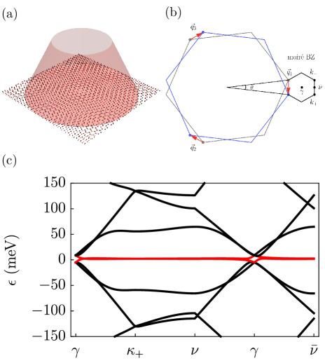
Figure 1: (Color online) a) Sketch of twisted bilayer graphene irradiated by circularly polarized light. (b) moiré Brilloiun zone. (c) Band structure for twisted bilayer graphene for $w_{0}=w_{1}=110$ meV, and $\theta=1.05^{\circ}$. The low-energy flat bands are highlighted in red.

The Hamiltonian in Eq. (1) describes only one valley degree of freedom. A full description of the system would incorporate the two graphene valleys. However, we only consider perturbations induced by light, which cannot induce processes that mix the two valleys. The Hamiltonian in the other valley is connected by a $C_{2}$ rotation Balents (2019). The symmetries of the continuum model Eq. (1) include $C_{3}$ rotational symmetry about the center of a AA region, $C_{2}\mathcal{T}$ symmetry (taking into account both valleys, the TBG presents time-reversal symmetry $\mathcal{T}$), and $M_{y}:y,k_{y}\to-y,-k_{y}$ mirror symmetry Hejazi et al. (2019); Balents (2019); Po et al. (2018). In the small-rotation limit, the angle dependence of the graphene sectors can be neglected, leading to an approximate particle-hole symmetry $\mathcal{C}$ Hejazi et al. (2019).

II.2 Driven twisted bilayer graphene

For the driven system, we assume that circularly polarized light is applied in a direction normal to the TBG plane as sketched in Fig. 1(a). Then, the light enters via minimal substitution as $k_{x}\to\tilde{k}_{x}(t)=k_{x}-A\cos(\Omega t)$, and $k_{y}\to\tilde{k}_{y}=k_{y}-A\sin(\Omega t)$ leaving the tunneling sector almost unaltered. The reason for this is simple. The inclusion of light in a tight binding model can be done via a Peirls substution for hoppings $t_{ij}\to e^{i\int_{R_{i}}^{R_{j}}\mathbf{A}d\mathbf{r}}t_{ij}$. The interlayer hopping is dominated by hopping between atoms that are almost exactly on top of each other - afterall other atoms are further away and the overlap between orbitals is smaller. Therefore for interlayer couplings mostly longitudinal components of $\mathbf{A}$ contribute in the line integral $\int_{R_{i}}^{R_{j}}\mathbf{A}d\mathbf{r}$. Circularly polarized light only has transverse components and therefore has little effect on interlayer couplings. The time-dependent Hamiltonian is

$$H(\mathbf{x},t)=\begin{pmatrix}h(-\theta/2,\mathbf{\tilde{k}}(t)-\kappa_{-})&T(\mathbf{x})\\ T^{\dagger}(\mathbf{x})&h(\theta/2,\mathbf{\tilde{k}}(t)-\kappa_{+})\end{pmatrix},$$ (5)

with $H(\mathbf{x},t+2\pi/\Omega)=H(\mathbf{x},t)$. The Floquet theorem Bukov et al. (2015); Eckardt and Anisimovas (2015b); Mikami et al. (2016b) exploits the discrete time-translational symmetry and allows one to write the wavefunctions as $|\psi(t)\rangle=e^{i\epsilon t}|\phi(t)\rangle$, where $|\phi(t+2\pi/\Omega)\rangle=|\phi(t)\rangle$ and $\epsilon$ is the quasienergy. Replacing $|\psi(t)\rangle$ into the Schrödinger equation leads to $[H(\mathbf{x},t)-i\partial_{t}]|\phi(t)\rangle=\epsilon|\phi(t)\rangle$, which governs the dynamics of the periodic system. The exact solution can be generically obtained either by constructing the Floquet evolution operator $U_{F}=\text{T}\exp\{-i\int^{2\pi/\Omega}_{0}H(s)ds\}=e^{-iH_{F}T}$ or by employing the extended-state picture. In the extended-state picture, we use the Fourier series $|\phi(t)\rangle=\sum_{n}e^{in\Omega t}|\phi_{n}\rangle$, which leads to $\sum_{m}\left(H^{(n-m)}+\delta_{n,m}\Omega m\right)|\phi_{m}\rangle=\epsilon|\phi_{n}\rangle$, defined in the infinite-dimensional Floquet-Hilbert space spanned by the direct product of the Hilbert space of the static system and the space spanned by a complete set of periodic functions. The Hamiltonian Fourier modes are given by $H^{(n)}=\int_{0}^{2\pi}d\tau/(2\pi)H(\tau)e^{-i\tau n}$, which can be derived by making the replacements

$$\begin{aligned} &f(\mathbf{k})\to f^{(n)}(\mathbf{k})=e^{-\frac{1}{3}i(2a_{0}k_{y}+3(\theta-\pi)n)}\left(1+2e^{ia_{0}k_{y}}\sin\left(\frac{a_{0}k_{x}}{\sqrt{3}}+\frac{2\pi n}{3}-\frac{\pi}{6}\right)\right)J_{n}\left(\frac{2Aa_{0}}{3}\right)\\ &T(\mathbf{x})\to T^{(n)}(\mathbf{x})=\delta_{n,0}T(\mathbf{x})\end{aligned},$$ (6)

in Eq. (1).

The two exact approaches outlined above are challenging to use in practice, and one usually has to employ approximations. In the following sections, we will employ a recently developed Vogl et al. (2020b) approach valid in the weak-drive limit and for arbitrary frequencies. Also, we will introduce improved methods to study the intermediate-amplitude drive regime valid in the high and intermediate frequency regimes.

III Weak drive regime

Thus far, most discussions of twisted bilayer graphene irradiated by circularly polarized light have focused on the high frequency limit. This is for practical reasons because the lower frequency regime, while it is more interesting and relevant for experiments, is also harder to treat using the existing theoretical tools. In Ref. Vogl et al., 2020b, we developed a method to address this issue in the weak driving limit. Here, we apply our method using a series of approximations necessary to make progress and gain some analytical insights into the low frequency regime.

If we are interested on the effects of the drive on the low-energy bands, small angles, and weak drives our original Hamiltonian can be approximated with $f(\mathbf{k})\approx f_{L}(\mathbf{k})=a_{0}e^{-i\frac{\theta}{2}}(k_{x}-ik_{y})$, in the vicinity of the graphene $K$ point. The reason we may Taylor expand for small momenta when the twist angle $\theta$ is small is because the moiré Brillouin zone is very small i.e. $k_{\theta}\ll k_{D}$. Non-linear corrections only become important for higher-energy bands. These higher-energy bands are in turn not relevant for the driven system in the weak-drive limit, since they couple weakly to the low-energy bands.

The time-dependent Hamiltonian within these approximations has the form

$$H(t)=H_{L}+\mathcal{P}e^{-i\Omega t}+\mathcal{P}^{\dagger}e^{i\Omega t},$$ (7)

where the monochromatic operator $\mathcal{P}=T^{-1}\int_{0}^{T}dsH(\mathbf{x},s)e^{i\Omega s}$ is given by

$$\mathcal{P}=-A\gamma a_{0}\begin{pmatrix}0&e^{i\theta/2}&0&0\\ 0&0&0&0\\ 0&0&0&e^{-i\theta/2}\\ 0&0&0&0\end{pmatrix},$$ (8)

and $H_{L}$ is the same as Eq. (1) just with $f(\mathbf{k})\to f_{L}(\mathbf{k})$ linearized momentum dependence.

For weak driving amplitudes $A$ and arbitrary frequency $\Omega$, the periodically driven systems can be described by the effective self-consistent time-independent Hamiltonian Vogl et al. (2020b)

$$H_{\mathrm{eff}}\approx H_{L}+P\frac{1}{\epsilon-H_{L}-\Omega}P^{\dagger}+P^{\dagger}\frac{1}{\epsilon-H_{L}+\Omega}P,$$ (9)

where $H_{0}$ is the time-averaged Hamiltonian, and $\epsilon$ are the quasienergies. For large frequency drives, we can apply a Van Vleck expansion and obtain the effective Hamiltonian Perfetto and Stefanucci (2015); Giovannini and Huebener (2019) $H_{\mathrm{eff}}=H_{L}+H_{\Omega}$, where the leading order correction is given by $H_{\Omega}=-\Delta\tau_{0}\otimes\sigma_{3}$, $\Delta=(A\gamma a_{0})^{2}/\Omega$, and $\sigma_{i}$, $\tau_{i}$ are the Pauli matrices in pseudo-spin and layer space, respectively. To keep the notation simple, in the remainder of the text we refer to the approximation $H_{eff}\approx H_{L}+[P^{\dagger},P]$ as the Van Vleck approximation.

Therefore, in the high-frequency limit, the main effect is the addition of the gap $\Delta$ in the quasienergy spectrum originating from the breaking of time-reversal symmetry $\mathcal{T}$. This gap is topologically non-trivial, and leads to topological Floquet flat bands with Chern number $C=4$ Katz et al. (2019); Li et al. (2019) which could serve as platforms to realize Floquet fractional Chern insulators Grushin et al. (2014); Li et al. (2019). The relatively large Chern number originates from spin and valley degeneracy Katz et al. (2019); Li et al. (2019).

In order to evaluate the effective Hamiltonian $H_{\text{eff}}$ for arbitrary frequency, we notice that the Brillouin zone has dimensions $k_{\theta}\propto\sin(\theta/2)$ and therefore the corresponding energy obeys $\hbar v_{F}k_{\theta}\ll w_{0,1}$ for sufficiently low angles. This is, for small angles, $T(\mathbf{x})$ introduces the dominant energy scale i.e. $\min\lVert T(\mathbf{x})\rVert\gg\lVert h(\mathbf{k})\rVert$, where $\lVert.\rVert$ is a matrix norm. This estimate can be written more precisely as

$$\sqrt{(\mathbf{k}-\kappa_{+})^{2}+(\mathbf{k}-\kappa_{-})^{2}}\ll 3\frac{w_{1}}{\hbar v_{F}}$$ (10)

if $w_{0}\approx w_{1}$. (Physically, this is a regime where the interlayer coupling are essential to the physics.) Therefore, for small enough angles and momenta that fulfill this inequality we may introduce the approximation $\left(\epsilon-H_{L}\pm\Omega\right)^{-1}\approx\left(\epsilon-H_{T}\pm\Omega\right)^{-1}$ where

$$H_{T}=\begin{pmatrix}0&T(\mathbf{x})\\ T^{\dagger}(\mathbf{x})&0\end{pmatrix}.$$ (11)

Replacing this approximation in the second and third terms of equation (9), we find the effective Hamiltonian $H_{\mathrm{eff}}=H_{0}+H_{\Omega}+\mathcal{O}\left(\left(\frac{A}{k_{D}}\right)^{3},\left(\frac{A}{k_{D}}\right)^{2}\frac{k_{\theta}}{k_{D}}\right)$, where the neglected terms that are third order in small parameters. We find that terms of order $\mathcal{O}\left(\frac{A}{k_{D}}\right)^{4}$ vanish. The leading-order correction to the Hamiltonian $H_{\Omega}$ has the following form

$$H_{\Omega}(\mathbf{x}) =V(\mathbf{x},\Omega)\mathcal{\tau}_{0}\otimes\sigma_{0}+U(\mathbf{x},\Omega)\tau_{3}\otimes\sigma_{0}+\frac{1}{2}\Delta_{1}(\mathbf{x},\Omega)(\tau_{0}+\tau_{3})\otimes\sigma_{3}+\frac{1}{2}\Delta_{2}(\mathbf{x},\Omega)(\tau_{0}-\tau_{3})\otimes\sigma_{3}$$

$$+\delta w_{0}(\mathbf{x},\Omega)\tau^{+}\otimes\sigma_{0}+\delta w^{*}_{0}(\mathbf{x},\Omega)\tau^{-}\otimes\sigma_{0}+\beta(\mathbf{x},\Omega)\tau^{+}\otimes\sigma_{3}+\beta^{*}(\mathbf{x},\Omega)\tau^{-}\otimes\sigma_{3}.$$ (12)

Equation (12) is the first main result of our work. The full expressions for each of the terms appearing in Eq. (12) are given in appendix A, and depend on the quasienergy, which was omitted explicitly for brevity. A perturbative approach generically generates long-range hopping terms as the frequency is arbitrarily decreased. The method here employed leads to the closed form in Eq. (12), which contains all the possible terms that can be generated by the drive, even in the low-frequency regime, defined as driving frequency $\Omega\lesssim W$ with $W\sim\mathrm{max}_{t}\left\lVert H(t)\right\rVert$. Conversely, we define the high-frequency regime for the moiré system as $\Omega>W\sim\mathrm{max}_{t}\left\lVert H(t)\right\rVert$.

Now, we discuss the origin and implications of each the new terms on the symmetries of the system. Due to the assumed approximations, the corrections to the Hamiltonian $H_{\Omega}(\mathbf{x})$ presents no momentum dependence and does not commute at different points in space, $\left[H_{\Omega}(\mathbf{x}),H_{\Omega}(\mathbf{x}^{\prime})\right]\neq 0$.

The first term, $V(\mathbf{x},\Omega)\mathcal{\sigma}_{0}\otimes\tau_{0}$, with $V(\mathbf{x},\Omega)\propto\mathcal{O}(\Omega^{-2})$, corresponds to an overall position-dependent potential which does not introduce new physics. The second term, $U(\mathbf{x},\Omega)\sigma_{0}\otimes\tau_{3}$, is a position-dependent interlayer bias with $U(x,y)=U(x,-y)$, $U(x,y)=-U(-x,y)$, and $U(x,y)\propto\mathcal{O}(\Omega^{-3})$. This term breaks mirror symmetry $M_{y}$ and allows a relative shift in quasienergy between the Dirac crossings at $\kappa_{\pm}$, as shown schematically in figure 2(a) for a spatially-uniform constant $U$. Because the $U(\mathbf{x},\Omega)$ is odd in the $x$-coordinate, $C_{2}\mathcal{T}$ and $C_{3}$ are also broken when taking the position dependence into account.

In Bernal-stacked bilayer graphene, a interlayer bias $U$ opens up a gap in the energy spectrum around the $K$ points Zhang et al. (2009); Mak et al. (2009). If we introduce a region in space where the sign of the interlayer bias changes, $U\rightarrow-U$, a domain wall forms where the gap inverts, leading to topologically protected helical (TPH) modes Qiao et al. (2011); Martin et al. (2008); Alden et al. (2013). In twisted bilayers, even though $U$ does not gap the spectrum, the moiré pattern alternating AB/BA regions leads to the formation of topological boundary modes even for spatially-homogeneous interlayer bias $U$ San-Jose and Prada (2013). Here, we obtained that circularly polarized light induces an interlayer potential $U(\mathbf{x},\Omega)$ in the low-frequency limit, which could induce the formation of topologically protected helical modes.

Next, the terms $\Delta_{1/2}(\mathbf{x},\Omega)(\tau_{0}\pm\tau_{3})\otimes\sigma_{3}$ with $\Delta_{1/2}(x,-y)=\Delta_{1/2}(x,y)$ and $\Delta_{2}(x,y)=\Delta_{1}(-x,y)$ break $M_{y}$, and $C_{2}\mathcal{T}$ symmetry, which protects the linear band crossing, leading to the opening of a gap at the $\kappa_{\pm}$ points in the mBZ. The $\Delta_{1/2}(\mathbf{x},\Omega)$ position dependence is relevant at order $\mathcal{O}(\Omega^{-3})$, and the asymmetry $\Delta_{1}\neq\Delta_{2}$ is relevant at order $\mathcal{O}(\Omega^{-4})$. When both TBG valleys are taken into account, this term breaks time-reversal symmetry $\mathcal{T}$ and leads to the formation of topologically non-trivial Floquet flat bands Li et al. (2019); Katz et al. (2019). The asymmetry $\Delta_{1}\neq\Delta_{2}$ leads to asymmetric gaps at the $\kappa_{\pm}$ points in the mBZ, as sketched in figure 2(b), where we plot the bands for TBG with a constant term of the form $\Delta_{1}(\tau_{0}\pm\tau_{3})\otimes\sigma_{3}$ added. The $\Delta_{1/2}(\mathbf{x},\Omega)$ position-dependence leads to breaking of $C_{3}$ symmetry.

The term $\delta w_{0}(\mathbf{x},\Omega)\tau^{+}\otimes\sigma_{0}$ (and its hermitian conjugate) where $\tau^{\pm}=1/2\left(\tau_{1}\pm i\tau_{2}\right)$, $\text{Re }\delta w_{0}(x,-y)=\text{Re }\delta w_{0}(x,y)$, $\text{Im }\delta w_{0}(x,-y)=-\text{Im }\delta w_{0}(x,y)$, $\delta w_{0}(-x,y)=\delta w_{0}(x,y)$ introduces a correction to the tunneling amplitude $w_{0}$, consistent with the symmetries of the static system, except $C_{3}$. $\delta w_{0}(\mathbf{x},\Omega)$ effectively renormalizes the Fermi velocity at the $\kappa_{\pm}$ points and can modify the position of the magic angles. To leading order, $\delta w_{0}(\mathbf{x},\Omega)\approx-(A\gamma a_{0}/\Omega)^{2}T_{11}(\mathbf{x})\cos(\theta)$, where $T_{11}(\mathbf{x},\Omega)$ corresponds to the diagonal entry of the tunneling matrix Eq. (3).

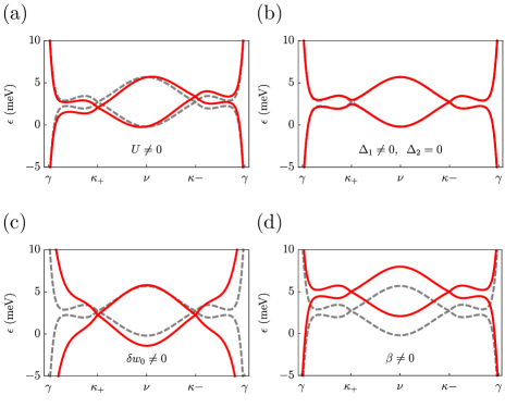
Figure 2: (Color online) Sketch of the individual effects of the new term generated by low-frequency and low-intensity circularly polarized light on the TBG quasienergies. The parameters used are $w_{0}=w_{1}=110$ meV, and $\theta=1.2^{\circ}$. The gray dashed curves correspond to the static case, while the red curve indicates the effect introduced by the non-zero perturbation introduced by light.

In figure 2(d), we schematically show the effect of this term in the Floquet bands. Controlled drive protocols to tune the Fermi velocity of the Floquet zone center flat quasienergy bands have previously been proposed Vogl et al. (2020a). For small angles, large drive frequency $\Omega$ and small quasienergies $\epsilon\ll\Omega$, this term constitutes the second most relevant correction after $\Delta_{1/2}(\mathbf{x},\Omega)$. An accurate description of the quasienergies $\epsilon$ near the Floquet zone center is challenging to achieve with high-frequency expansions such as the Magnus expansion, which highlights the strength of our approach. Crucially, the physics of the Floquet bands near the Floquet zone center is not obfuscated by negligible contributions from static high-energy bands which do not hybridize due to the weak drives considered here. Finally, the correction to the interlayer tunneling $\delta w_{0}(\mathbf{x},\Omega)$ is bears resemblence to effects one would expect from the relaxation of the driven lattice. Particularly, this term only affects the AA-type interlayer coupling $w_{0}$, which reduces. One could observe a similar effect if the size of AA-type patches were to shrink, which would also lead to the reduction in $w_{0}$. Secondly if the interlayer distance in AA stacked regions increased, this would also lead to a similar reduction of $w_{0}$. Therefore the periodic drive is able to mimic these effects.

Finally, we address the term $\beta(\mathbf{x},\Omega)\tau^{+}\otimes\sigma_{3}$ (and its hermitian conjugate) with real-space transformation properties $\beta(-x,y)=\beta(x,y)$, $\text{Re}\beta(x,-y)=\text{Re}\beta(x,y)$, and $\text{Im}\beta(x,-y)=-\text{Im}\beta(x,y)$. To leading order, $\beta(\mathbf{x},\Omega)=i(A\gamma a_{0}/\Omega)^{2}T_{11}(\mathbf{x})\sin\theta+O(\Omega^{-3})$. Neglecting its position dependence, $\beta$ preserves $C_{2}\mathcal{T}$ and $M_{y}$. Taking the position dependence into account, $\beta(\mathbf{x})$ breaks both $C_{2}\mathcal{T}$ and $M_{y}$. Physically $\beta(\mathbf{x},\Omega)$ can be interpreted as a pseudo-spin dependent tunneling term. Therefore, in the weak-drive, small angle and low-frequency regime, circularly polarized light can introduce a collection of symmetry-breaking processes beyond the reach of the high-frequency limit.

In addition to the small angle limit where Eq.(10) is fulfilled let us also consider the opposite limit

$$\sqrt{(\mathbf{k}-\kappa_{+})^{2}+(\mathbf{k}-\kappa_{-})^{2}}\gg 3\frac{w_{1}}{\hbar v_{F}}$$ (13)

where $\left(\epsilon-H_{L}\pm\Omega\right)^{-1}\approx\left(\epsilon-H_{g}\pm\Omega\right)^{-1}$ with

$$H_{g}=\begin{pmatrix}h(-\theta/2,\mathbf{k}-\kappa_{-})&0\\ 0&h(\theta/2,\mathbf{k}-\kappa_{+})\end{pmatrix}.$$ (14)

In this case we find that $H_{\mathrm{eff}}=H_{0}+H_{\Omega}+\mathcal{O}\left(\left(\frac{A}{k_{D}}\right)^{3},\left(\frac{A}{k_{D}}\right)^{2}\frac{w_{1,2}}{\gamma}\right)$

$$H_{\Omega}(\mathbf{k})=V(\mathbf{k},\Omega)\mathcal{\tau}_{0}\otimes\sigma_{0}+U(\mathbf{k},\Omega)\tau_{3}\otimes\sigma_{0}+\frac{1}{2}\Delta_{1}(\mathbf{k},\Omega)(\tau_{0}+\tau_{3})\otimes\sigma_{3}+\frac{1}{2}\Delta_{2}(\mathbf{k},\Omega)(\tau_{0}-\tau_{3})\otimes\sigma_{3}$$ (15)

The gaps are given as

$$\frac{\Delta_{1/2}(\mathbf{k},\Omega)}{A^{2}a_{0}^{2}\gamma^{2}}=\frac{\Omega\left(\epsilon^{2}-\Omega^{2}+\left|f_{1/2}(\mathbf{k}))\right|^{2}\right)}{\Lambda_{1/2}(\epsilon,\mathbf{k},\Omega)},$$ (16)

the interlayer bias is

$$\frac{U(\mathbf{k},\Omega)}{A^{2}a_{0}^{2}\gamma^{2}}=-\frac{\epsilon}{2}\sum_{m=1}^{2}(-1)^{m}\frac{\epsilon^{2}-\Omega^{2}-\left|f_{m}(\mathbf{k}))\right|^{2}}{\Lambda_{m}(\epsilon,\mathbf{k},\Omega)}$$ (17)

and

$$\frac{V(\mathbf{k},\Omega)}{A^{2}a_{0}^{2}\gamma^{2}}=\frac{\epsilon}{2}\sum_{m=1}^{2}\frac{\epsilon^{2}-\Omega^{2}-\left|f_{m}(\mathbf{k}))\right|^{2}}{\Lambda_{m}(\epsilon,\mathbf{k},\Omega)}.$$ (18)

where $f_{1/2}(\mathbf{k})=f(R(\mp\theta/2)(\mathbf{k}-\kappa_{\mp}))$, with the property $|f_{1/2}(k_{x},-k_{y})|^{2}=|f_{2/1}(\mathbf{k})|^{2}$, and

$$\Lambda_{1/2}(\epsilon,\mathbf{k},\Omega)=\prod_{m=1}^{2}\left(\left|f_{1/2}(\mathbf{k}))\right|^{2}-(\epsilon+(-1)^{m}\Omega)^{2}\right),$$ (19)

with $\Lambda_{1/2}(\epsilon,(k_{x},-k_{y}),\Omega)=\Lambda_{2/1}(\epsilon,\mathbf{k},\Omega)$. This property implies that $V((k_{x},-k_{y}),\Omega)=V(\mathbf{k},\Omega)$, $U((k_{x},-k_{y}),\Omega)=-U(\mathbf{k},\Omega)$, and $\Delta_{1/2}((k_{x},-k_{y}),\Omega)=\Delta_{2/1}(\mathbf{k},\Omega)$. Furthermore, $U(\mathbf{k},\Omega)$, $V(\mathbf{k},\Omega)$, and $\Delta_{1/2}(\mathbf{k},\Omega)$ are invariant under a $C_{3}$ rotation of the momentum, since $|f_{1/2}(C_{3}\{\mathbf{k}\})|^{2}=|f_{1/2}(\mathbf{k})|^{2}$. We find that not all terms appearing in Eq.(12) valid in the limit Eq.(10) are generated, and that they are momentum-dependent rather than position-dependent. A summary of the results for what symmetries get broken by the different terms is given in Table 1.

	$C_{2}{\cal T}$	$C_{3}$	$M_{y}$
$U$	$\checkmark$	$\checkmark$	x
$U(\mathbf{x})$	x	x	x
$U(\mathbf{k})$	$\checkmark$	$\checkmark$	$\checkmark$
$\Delta$	x	$\checkmark$	x
$\Delta(\mathbf{x})$	x	x	x
$\Delta(\mathbf{k})$	x	$\checkmark$	x
$\delta\omega_{0}$	$\checkmark$	x	$\checkmark$
$\delta\omega_{0}(\mathbf{x})$	$\checkmark$	x	$\checkmark$
$\beta$	$\checkmark$	x	$\checkmark$
$\beta(\mathbf{x})$	x	x	x

Table 1: This table lists the symmetries that are broken for the different terms that can be generated for the case of position dependence, momentum dependence, or if the term is constant. A checkmark means that the symmetry is preserved, while a cross that symmetry is broken.

The more general case, where neither condition Eq.(10) nor the opposite Eq.(13) are fulfilled, we can use the general form of $\mathcal{P}$ to find that an effective Hamiltonian has the same structure as Eq.(12). However, all terms have an additional momentum dependence (e.g. $\Delta_{1,2}(\mathbf{x},\Omega)\to\Delta_{1,2}(\mathbf{x},\mathbf{k},\Omega)$ etc.). While it is possible to determine that $H_{\Omega}$ has this structure generally, the coefficients are too cumbersome to compute and are therefore not discussed.

IV Intermediate drive regime

IV.1 Issues with the usual form of the rotating frame transformation

A standard approach for treating systems subjected to intermediately strong drives and intermediate frequencies is applying a rotating frame transformation before the use of a high frequency Magnus expansion Vogl et al. (2019a, b); Bukov et al. (2015). To accomplish when a Hamiltonian has the form $H(t)=H_{0}+\lambda V(t)$, one applies the unitary transformation $U(t)=e^{-i\lambda\int dtV(t)}$ to remove $V(t)$ to lowest order. A large term $\lambda V(t)$ in the Hamiltonian can be traded this way for strongly oscillating terms Bukov et al. (2015). This approach allows treating regimes where $\lambda$ is too large for a Magnus approximation to be applicable, and is known to give results that are more reliable than the Magnus expansion Vogl et al. (2019a, b); Bukov et al. (2015).

First, we consider the simpler driven Dirac model

$$H_{\mathrm{D}}=\begin{pmatrix}0&k_{x}-ik_{y}+\lambda e^{-i\Omega t}\\ k_{x}+ik_{y}+\lambda e^{i\Omega t}&0\end{pmatrix},$$ (20)

which also describes the upper layer of twisted bilayer graphene near the K point for $w_{1}=w_{0}=0$, $\gamma=a_{0}=1$, $\kappa_{\pm}=0$ and very small $\theta$.

Application of the unitary transformation $U(t)=e^{-i\lambda\int dtV(t)}$ followed by a zeroth order Magnus approximation leads to a Hamiltonian of the form

$$\begin{aligned} &H_{\mathrm{eff,D}}=(\mathbf{B}+R_{y}(\tau)(\kappa_{1},\kappa_{2},0)^{T})\cdot\sigma\\ \end{aligned},$$ (21)

where $R_{y}(\tau)$ is a rotation matrix around the y-axis by an angle

$$\tau=\tan^{-1}\left(\frac{sJ_{1}\left(s\right)}{sJ_{0}\left(s\right)-J_{1}\left(s\right)+\frac{s}{2}}\right),$$ (22)

$s=\frac{4\lambda}{\Omega}$, and $J_{n}(x)$ is the n-th Bessel function of the first kind. The Hamiltonian has a constant field-like part with

$$B_{x} =\frac{\lambda}{2}-\lambda\left(J_{0}\left(s\right)-\frac{J_{1}\left(s\right)}{s}\right),$$ (23)

$$B_{y} =0,$$ (24)

$$B_{z} =\frac{1}{s}\lambda\left(J_{0}\left(s\right)-1\right)-\lambda J_{1}\left(s\right),$$ (25)

and momenta given by

$$\bar{k}_{x} =k_{x}(s+2sJ_{0}(s)-2J_{1}(s))$$

$$\times\frac{\sqrt{\frac{2s^{2}J_{0}(s)(1-2J_{2}(s))+s^{2}(1-2J_{2}(s))+4\left(s^{2}+1\right)J_{1}(s){}^{2}}{(s+2sJ_{0}(s)-2J_{1}(s)){}^{2}}}}{2s},$$ (26)

$$\bar{k}_{y} =\frac{1}{2}k_{y}\left(\frac{2J_{1}(s)}{s}+1\right).$$ (27)

By inspecting $\bar{k}_{x}$ and $\bar{k}_{y}$, we realize that $k_{x}$ and $k_{y}$ are not treated on equal grounds in this approximation. Specifically, the Fermi velocity has become anisotropic. The quasi-energy spectrum is not rotationally symmetric for large driving $\lambda$. Specifically if we expand $\bar{k}_{x,y}\approx k_{x,y}\left(1-\frac{s^{2}}{16}\mp\frac{s^{4}}{384}\right)$ we see that the anisotropic behaviour appears at fourth order in $s$- that is for relatively large $\lambda$. This is in qualitative disagreement with an exact numerical calculations, which present rotationally-symmetric quasi-energies. Since the problem already appears in the Dirac case, we can therefore expect the rotating frame approximation to also produce unphysical artifacts for the more complicated problem of twisted bilayer graphene. It is important to note that the same type of unphysical anisotropy already appears on the level of a first order Magnus expansion Eckardt and Anisimovas (2015a). Therefore, a more careful partial resummation of the Magnus expansion is needed.

IV.2 A better choice of unitary transformation

In order to avoid introducing unphysical terms in the effective Floquet Hamiltonian, we write the time-dependent Hamiltonian as $H(t)=H_{0}+\lambda V_{1}(t)+\lambda V_{2}(t)$ with $[V_{i}(t),V_{i}(t_{1})]=0$ and apply the modified unitary transformation $U(t)=e^{-i\int dtV_{1}(t)}e^{-i\int dtV_{2}(t)}$ with $V_{1}(t)=\lambda\cos(\Omega t)\sigma_{1}$ and $V_{2}(t)=\lambda\sin(\Omega t)\sigma_{2}$. There is an associated arbitrariness in the exact form of this unitary transformation arising from the choice of $V_{1}$ and $V_{2}$. However, given our implicit Floquet gauge choice $t^{*}=0$, in a time-ordered exponential that removes all of $V_{1}+V_{2}$ we make the smaller error by removing a $V_{1}$ first, that is the larger of the two at $t^{*}=0$. In the Dirac model this choice can be justified even better better apostiori by realizing that it restores the rotational invariance in momentum space.

We will make an analogous choice of unitary transformations for the TBG case in section IV.4, where we will explicitly demonstrate that the anisotropy in the Fermi velocity is not present.

IV.3 Improved Van Vleck approximation

In this section, we identify a procedure to improve the Van Vleck expansion used to obtain an effective Floquet Hamiltonian which we will use as a baseline to compare our improved rotating frame effective Hamiltonian.

For small twist angles $\theta$ it is sensible to treat $\mathbf{k}$ as a small parameter because the dimensions of the moiré Brillouin zone are proportional to $\sin(\theta/2)$. Therefore, we may approximate $f(\mathbf{k}-\mathbf{A})\approx f(-\mathbf{A})+(k_{x}(\partial_{k_{x}}f)(-\mathbf{A})+k_{y}(\partial_{k_{y}}f)(-\mathbf{A}))$. In the weak-strength drive regime, $A\ll a_{0}$, we employed a simple Taylor expansion. However, in order to capture the effect of stronger drives, we need to improve our approach. For this, we perform a Fourier series in terms of $e^{i\Omega nt}$ instead. The result to first order in Fourier components has the form $f(\mathbf{k}-\mathbf{A})\approx a_{0}(k_{x}-ik_{y})J_{0}(2a_{0}A/3)-3J_{1}(2a_{0}A/3)e^{i\Omega t}-a_{0}(k_{x}+ik_{y})J_{1}(2a_{0}A/3)e^{-i\Omega t}$. For $2a_{0}A/3$ not too large compared with unit, $J_{1}(2a_{0}A/3)\ll 1$. Therefore, terms like $k_{i}J_{1}(2a_{0}A/3)$ are higher order and can be neglected. We will thus work with the approximation

$$f(\mathbf{k}-\mathbf{A})\approx a_{0}(k_{x}-ik_{y})J_{0}\left(\frac{2a_{0}A}{3}\right)-3J_{1}\left(\frac{2a_{0}A}{3}\right)e^{i\Omega t}.$$ (28)

This type of approximation is reasonable for small angles and $2a_{0}A/3\lesssim 1$.

After application of this approximation we can readily improve on the Van Vleck approximation, which we will use to compare our results from the rotating wave approximation. The effective Floquet Hamiltonian keeps the same structure as previously obtained, $H^{\text{vV}}_{\mathrm{eff}}=H_{L}-\Delta\tau_{0}\otimes\sigma_{3}$ with gap

$$\Delta=\frac{9\gamma^{2}}{\Omega}J_{1}\left(\frac{2Aa_{0}}{3}\right)^{2}$$ (29)

and a renormalized Fermi velocity

$$\tilde{v}_{F}=v_{F}J_{0}\left(\frac{2Aa_{0}}{3}\right).$$ (30)

IV.4 Rotating frame Hamiltonian

In this section, we will derive an effective Floquet Hamiltonian using a rotating frame approach, $H^{R}_{\text{eff}}$, with an improved unitary transformation. Then, we compare the quasienergies obtained with the ones derived from the Van Vleck Hamiltonian $H^{\text{vV}}_{\mathrm{eff}}$.

We write the time-dependent Hamiltonian for twisted bilayer graphene as $H(t)=H_{L}+V_{1}(t)+V_{2}(t)$, where the time dependent potentials are given as

$$V_{1}(t) =-3J_{1}(2a_{0}A/3)\cos(\Omega t)\begin{pmatrix}\sigma_{1}^{(-\theta/2)}&0\\ 0&\sigma_{1}^{(\theta/2)}\end{pmatrix}$$ (31)

$$V_{2}(t) =-3J_{1}(2a_{0}A/3)\sin(\Omega t)\begin{pmatrix}\sigma_{2}^{(-\theta/2)}&0\\ 0&\sigma_{2}^{(\theta/2)}\end{pmatrix},$$ (32)

where $\sigma_{i}^{\theta}=e^{-i\frac{\theta}{2}\sigma_{3}}\sigma_{i}e^{i\frac{\theta}{2}\sigma_{3}}$. After applying the unitary transformation $U(t)=e^{-i\int dtV_{1}(t)}e^{-i\int dtV_{2}(t)}$ and after taking an average over one period $2\pi/\Omega$ we find the following effective Hamiltonian for twisted bilayer graphene that is subjected to circularly polarized light

$$\begin{aligned} &H^{R}_{\text{eff}}=R\begin{pmatrix}(e^{-i\frac{\theta}{2}}\tilde{v}_{F}(\mathbf{k}-\mathbf{\kappa}_{-})+\Delta\hat{e}_{z})\cdot\bm{\sigma}&\tilde{T}(\mathbf{r})\\ \tilde{T}^{\dagger}(\mathbf{r})&(e^{i\frac{\theta}{2}}\tilde{v}_{F}(\mathbf{k}-\mathbf{\kappa}_{+})+\Delta\hat{e}_{z})\cdot\bm{\sigma}\end{pmatrix}R^{\dagger}\end{aligned},$$ (33)

where $\hat{e}_{z}$ is a unit vector in z-direction and $\sigma$ is a vector of Pauli matrices. The unitary transformation

$$R=\left(\begin{array}[]{cc}e^{\frac{3\gamma J_{1}\left(\frac{2Aa_{0}}{3}\right)}{\Omega}i\sigma_{2}^{(\theta/2)}}&0\\ 0&e^{\frac{3\gamma J_{1}\left(\frac{2Aa_{0}}{3}\right)}{\Omega}i\sigma_{y}^{(-\theta/2)}}\\ \end{array}\right),$$ (34)

allows us to cast the Hamiltonian in more readable form. From this unitary transformation, one can directly identify the origin of the spurious anisotropy in momentum that one would find in a Magnus expansion approach. Particularly, an expansion of $R$ for large frequencies unavoidably leads to such issue.

We find that the Fermi velocity has been renormalized to

$$\tilde{v}_{F}=v_{F}J_{0}\left(\frac{2Aa_{0}}{3}\right)J_{0}\left(\frac{6\gamma J_{1}\left(\frac{2Aa_{0}}{3}\right)}{\Omega}\right).$$ (35)

In figure 3, we show a plot of the Fermi velocity and compare with to the Fermi velocity from the improved Van Vleck approximation $H^{\text{vV}}_{\text{eff}}$. We find that the renormalization of the Fermi velocity is $\sim 10\%$ in some regions even for relatively high frequencies.

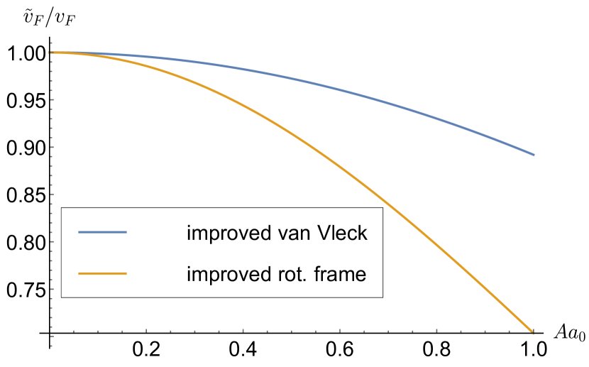
Figure 3: Fermi velocity normalized to bare $v_{F}$ for relatively high frequency drives $\frac{\gamma}{\Omega}=\frac{1}{2}$. In blue, we show the Van Vleck result and in orange the renormalized result employing our improved rotating frame approximation.

Furthermore, in $H^{R}_{\text{eff}}$, the quasienergy gap that is renormalized to

$$\tilde{\Delta}=\frac{3}{\sqrt{2}}\gamma J_{1}\left(\frac{2Aa_{0}}{3}\right)J_{1}\left(\frac{6\sqrt{2}\gamma J_{1}\left(\frac{2Aa_{0}}{3}\right)}{\Omega}\right).$$ (36)

A comparison with the Van Vleck result is shown in figure 4.

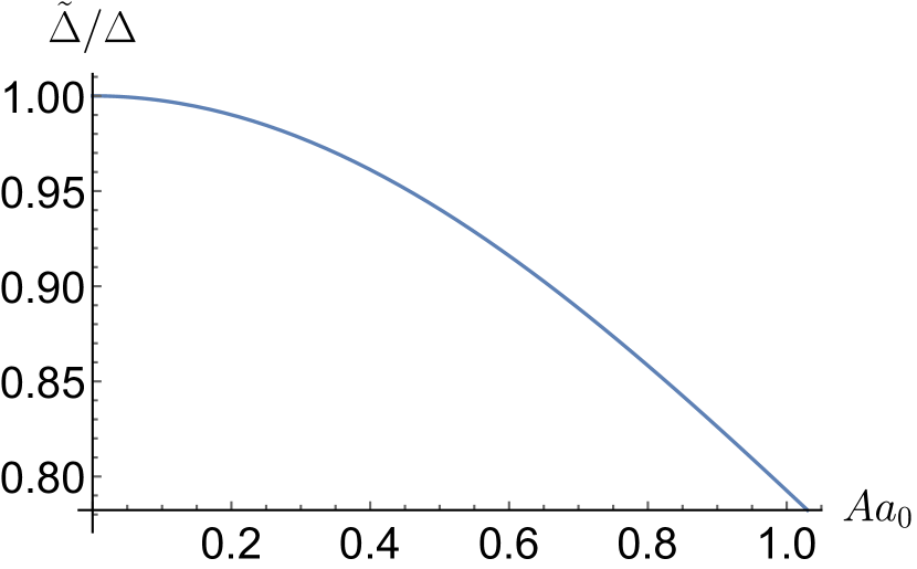
Figure 4: Ratio $\tilde{\Delta}/\Delta$ of the renormalized gap $\tilde{\Delta}$ and the gap of from the Van Vleck $\Delta$ for driving frequency $\Omega=2\gamma$.

We find that also in this case that there is considerable difference ($\sim 10\%$ in some regions in parameter space) even for relatively large driving frequencies $\Omega=2\gamma$.

The most striking difference between $H^{\text{vV}}_{\text{eff}}$ and $H^{\text{R}}_{\text{eff}}$ appears in the tunneling sector, where $H^{\text{R}}_{\text{eff}}$ contains renormalized interlayer hopping

$$\tilde{T}(\mathbf{x})=\sum_{l=-1}^{1}e^{-i\mathbf{b}_{l}\mathbf{x}}(\tilde{T}_{l}-i\beta\sigma_{3})$$ (37)

$$\tilde{T}_{n}=\tilde{w}_{0}\mathbb{1}_{2}+\tilde{w}_{1}\left(\cos\left(\frac{2\pi n}{3}\right)\sigma_{1}+\sin\left(\frac{2\pi n}{3}\right)\sigma_{2}\right),$$

with

$$\tilde{w}_{1} =w_{1}J_{0}\left(\frac{6\gamma J_{1}\left(\frac{2Aa_{0}}{3}\right)}{\Omega}\right)$$ (38)

$$\tilde{w}_{0} =w_{0}\left[1+\sin^{2}\left(\frac{\theta}{2}\right)\left(J_{0}\left(\frac{6\sqrt{2}\gamma J_{1}\left(\frac{2Aa_{0}}{3}\right)}{\Omega}\right)-1\right)\right],$$ (39)

and a new imaginary term in the AA interlayer coupling

$$\beta=\frac{1}{2}\sin(\theta)\left(1-J_{0}\left(\frac{6\sqrt{2}\gamma J_{1}\left(\frac{2Aa_{0}}{3}\right)}{\omega}\right)\right).$$ (40)

In the notation of the previous section III the new coupling term enters as $-i\beta\tau^{+}\otimes\sigma_{3}$ and is position dependent. The new dynamically-generated tunneling component $\beta$ breaks $C_{3}$, the approximate particle-hole symmetry $\mathcal{C}$, $C_{2}\mathcal{T}$ and reflection $M_{y}$ symmetries.

In figure 5, we compare our results using $H^{R}_{\text{eff}}$ in Eq. (33) to exact numeric results obtained employed an extended space approach Eckardt and Anisimovas (2015a). We use the improved Van Vleck approximation $H^{\text{vV}}_{\mathrm{eff}}=H_{L}-\Delta\tau_{0}\otimes\sigma_{3}$ as a benchmark. We find that the Van Vleck approximation is only valid until $a_{0}A\approx 0.4$, while the new approximation works well until $a_{0}A\approx 0.8$. The approximation therefore has double the range of validity and therefore is more reliable.

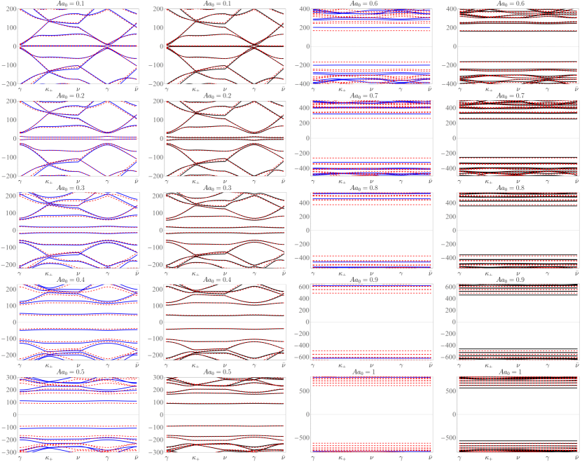
Figure 5: Quasi-energy band structure. The dashed red curves correspond to the exact result, in blue the improved Van Vleck approximation and in black the rotation frame transformation. The parameters used are $\Omega=2\gamma$, $w_{1}=w_{0}=110$ meV, $\gamma=2364$ meV and $\theta=1.05^{\circ}$.

The same observation can be made a bit more lucidly - albeit losing much information- if we compute the relative error of the gap at the $K$ point $(g_{\mathrm{exact}}-g_{\mathrm{approx}})/g_{\mathrm{exact}}$, where $g_{\mathrm{exact}}$ is the “exact” numerical gap at the $K$ point and $g_{\mathrm{approx}}$ is the gap for an approximation. For both approximations the result is shown in Fig. 6 below.

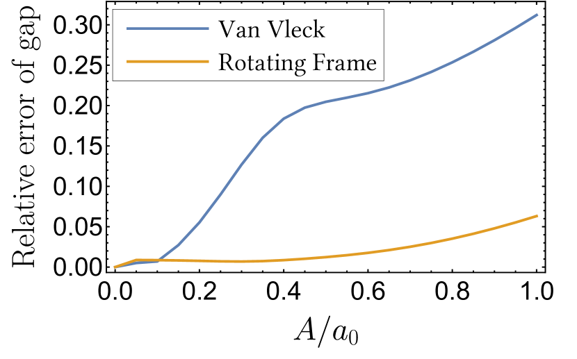
Figure 6: Plot of the relative error for the gap at the $K$ point of the moiré Brillouin zone. In blue we present our results from the Van Vleck approximation and in orange the results from our improved rotating frame approximation.

It is clear from both plots that the rotating frame approximation derived in this paper is far more reliable than the Van Vleck approximation.

V Conclusion and Outlook

We have introduced two new effective Floquet Hamiltonians that describe twisted bilayer graphene under the influence of circularly polarized light. The Hamiltonians are applicable in the regimes where the ordinary Van Vleck approximation fails. We found that the weak drive strength Hamiltonian, valid even in the low-frequency regime, gives insight into which new terms a periodic drive can generate well beyond the regime of validity of any other approximation scheme. The usefulness of these scheme is limited by the challenge imposed by the complexity of the terms derived and the self-consistent nature of the low-frequency regime. An important physical effect of the drive in these regime is a renormalization of the interlayer-coupling of the AA-type. This makes it possible to mimic the effects of some otherwise difficult to achieve structural reorganizations - for instance a change in the distance between the two graphene layers that only appears in AA regions.

The rotating frame Hamiltonian, valid for strong drives and intermediate drive frequencies reveals that the gap at the Floquet zone center, the Fermi velocity, and the interlayer-coupling strengths are renormalized. This effective Hamiltonian is useful for numerical implementation of the quasienergy band structure and posses a wide range of validity. This would make it useful for applications where an extended space calculation may be too expensive. For instance if one studies the effect of disorder additional disorder averages make calculations expensive and therefore it might be more feasible to do these calculations using the effective Hamiltonian we presented rather than resorting to a full treatment in an extended space picture.

VI Acknowledgements

We thank Fengcheng Wu for useful discussions. This research was primarily supported by the National Science Foundation through the Center for Dynamics and Control of Materials: an NSF MRSEC under Cooperative Agreement No. DMR-1720595. Partial support was from NSF Grant No. DMR-1949701.

Appendix A The low frequency Hamiltonian

The precise form of the effective low frequency Hamiltonian is given as

$$H_{\mathrm{eff}}=H_{0}+H_{\Omega}+\mathcal{O}\left(\left(\frac{A}{k_{D}}\right)^{4},\left(\frac{A}{k_{D}}\right)^{2}\frac{k_{\theta}}{k_{D}}\right)$$ (41)

$$H_{\Omega}=A^{2}\gamma^{2}a_{0}^{2}\left(\begin{array}[]{cccc}W_{1}^{-}&0&F_{-}&0\\ 0&W_{2}^{+}&0&F_{+}\\ F_{-}^{*}&0&W_{2}^{-}&0\\ 0&F_{+}^{*}&0&W_{1}^{+}\\ \end{array},\right)$$

$$F_{\pm}=\frac{e^{\mp i\theta}\left((\epsilon\pm\Omega)^{2}T_{11}(\mathbf{x})-\text{det}(T(\mathbf{x}))T_{11}^{*}(\mathbf{x})\right)}{D(\epsilon\pm\Omega)},$$

$$W_{n}^{\pm}=-\frac{(\epsilon\pm\Omega)[(\epsilon\pm\Omega)^{2}-w_{0}^{2}\lambda-w_{1}^{2}\tau_{n}]}{D(\epsilon\pm\Omega)},$$

$$\lambda=1+4\cos\left(\frac{\sqrt{3}x_{1}^{\theta}}{2}\right)\left(\cos\left(\frac{\sqrt{3}x_{1}^{\theta}}{2}\right)+\cos\left(\frac{3x_{2}^{\theta}}{2}\right)\right),$$

$$\tau_{n}=3-4\cos\left(\frac{3x_{2}^{\theta}}{2}\right)\sin\left(\frac{\pi}{6}-\frac{\sqrt{3}}{2}(-1)^{n}x_{1}^{\theta}\right),$$

$$\hskip 22.76228pt-2\sin\left((-1)^{n}\sqrt{3}x_{1}^{\theta}+\frac{\pi}{6}\right);\quad x_{i}^{\theta}=x_{i}k_{\theta},$$

$$D(\epsilon)=-\epsilon^{4}+\epsilon^{2}\mathrm{Tr}(T^{\dagger}(\mathbf{x})T(\mathbf{x}))-\left|\text{detT}\right|^{2},$$

The quantities in the main text can be derived from here. We find that the intralayer gaps are given as $\Delta_{1}(\mathbf{x})=\frac{1}{2}(W_{1}^{-}-W_{2}^{+})$, $\Delta_{2}(\mathbf{x})=\frac{1}{2}(W_{2}^{-}-W_{1}^{+})$. A Taylor series reveals

$$\begin{aligned} &\frac{\Delta_{n}(\mathbf{x})}{A^{2}\gamma^{2}a_{0}^{2}}=-\frac{1}{\Omega}-\frac{\epsilon^{2}+\mathrm{Tr}(T^{\dagger}T)-w_{0}^{2}\lambda-w_{1}^{2}\frac{\tau_{1}+\tau_{2}}{2}}{\Omega^{3}}\\ &\hskip 39.83368pt-(-1)^{n}\frac{3\epsilon w_{1}^{2}(\tau_{1}-\tau_{2})}{2\Omega^{4}}+\mathcal{O}(\Omega^{-5})\end{aligned}.$$ (42)

The interlayer bias is given as $U(\mathbf{x})=\frac{1}{4}(W_{1}^{-}-W_{1}^{+}-W_{2}^{-}+W_{2}^{+})$. A series expansion is

$$\frac{U(\mathbf{x})}{A^{2}\gamma^{2}a_{0}^{2}}=\frac{(\tau_{1}-\tau_{2})w_{1}^{2}}{2\Omega^{3}}+\mathcal{O}(\Omega^{-5}).$$ (43)

As last term from the diagonal block we find the overall potential of form $V(\mathbf{x})=\frac{1}{4}(W_{1}^{-}+W_{1}^{+}+W_{2}^{-}+W_{2}^{+})$, which is expanded as

$$\frac{V(\mathbf{x})}{A^{2}\gamma^{2}a_{0}^{2}}-\mathcal{O}(\Omega^{-5})=-\frac{\epsilon}{\Omega^{2}}$$ (44)

$$-\frac{\epsilon\left(2\epsilon^{2}+6(\mathrm{Tr}(T^{\dagger}T)-\lambda w_{0}^{2})-3w_{1}^{2}(\tau_{1}+\tau_{2})\right)}{2\Omega^{4}}.$$

Notably the lowest order term is just a constant shift in quasi-energy.

On the off-diagonal blocks we find the interlayer hopping strength $\delta w_{0}(\mathbf{x})=\frac{1}{2}(F_{-}+F_{+})$, which to lower order in $\Omega^{-1}$ is

$$\begin{aligned} &\frac{\delta w_{0}(\mathbf{x})}{A^{2}\gamma^{2}a_{0}^{2}}-\mathcal{O}(\Omega^{-5})=-\frac{T_{11}\cos(\theta)}{\Omega^{2}}-\frac{2i\epsilon T_{11}\sin(\theta)}{\Omega^{3}}\\ &-\frac{\cos(\theta)\left(T_{11}(3\epsilon^{2}+\mathrm{tr}(T^{\dagger}T))-T_{11}^{*}\mathrm{det}(T)\right)}{\Omega^{4}}\end{aligned}.$$ (45)

Furthermore we find that the interlayer hopping has a bias $\beta=\frac{1}{2}(F_{-}-F_{+})$, which to low orders has the form

$$\begin{aligned} &\frac{\beta(\mathbf{x})}{A^{2}\gamma^{2}a_{0}^{2}}-\mathcal{O}(\Omega^{-5})=-\frac{iT_{11}\sin(\theta)}{\Omega^{2}}-\frac{2T_{11}\epsilon\cos(\theta)}{\Omega^{3}}\\ &-\frac{i\sin(\theta)\left(T_{11}\left(3\epsilon^{2}+\mathrm{Tr}(T^{\dagger}T)\right)-T_{11}^{*}\mathrm{det}(T)\right)}{\Omega^{4}}\end{aligned}.$$ (46)

References

- Wu et al. (2018) Fengcheng Wu, A.H. MacDonald, and Ivar Martin, “Theory of phonon-mediated superconductivity in twisted bilayer graphene,” Phys. Rev. Letters 121 (2018).
- Cao et al. (2018a) Yuan Cao, Valla Fatemi, Shiang Fang, Kenji Watanabe, Takashi Taniguchi, Efthimios Kaxiras, and Pablo Jarillo-Herrero, “Unconventional superconductivity in magic-angle graphene superlattices,” Nature 556, 43–50 (2018a), article.
- Tsai et al. (2019) Kan-Ting Tsai, Xi Zhang, Ziyan Zhu, Yujie Luo, Stephen Carr, Mitchell Luskin, Efthimios Kaxiras, and Ke Wang, “Correlated superconducting and insulating states in twisted trilayer graphene moire of moire superlattices,” (2019), arXiv:1912.03375 [cond-mat.mes-hall] .
- Codecido et al. (2019) Emilio Codecido, Qiyue Wang, Ryan Koester, Shi Che, Haidong Tian, Rui Lv, Son Tran, Kenji Watanabe, Takashi Taniguchi, Fan Zhang, Marc Bockrath, and Chun Ning Lau, “Correlated insulating and superconducting states in twisted bilayer graphene below the magic angle,” Science Advances 5 (2019).
- Yankowitz et al. (2019) Matthew Yankowitz, Shaowen Chen, Hryhoriy Polshyn, Yuxuan Zhang, K. Watanabe, T. Taniguchi, David Graf, Andrea F. Young, and Cory R. Dean, “Tuning superconductivity in twisted bilayer graphene,” Science 363, 1059–1064 (2019).
- Chichinadze et al. (2019) Dmitry V. Chichinadze, Laura Classen, and Andrey V. Chubukov, “Nematic superconductivity in twisted bilayer graphene,” (2019), arXiv:1910.07379 [cond-mat.supr-con] .
- Chou et al. (2019) Yang-Zhi Chou, Yu-Ping Lin, Sankar Das Sarma, and Rahul M. Nandkishore, “Superconductor versus insulator in twisted bilayer graphene,” Phys. Rev. B 100 (2019).
- Guinea and Walet (2018) Francisco Guinea and Niels R. Walet, “Electrostatic effects, band distortions, and superconductivity in twisted graphene bilayers,” Proceedings of the National Academy of Sciences 115, 13174–13179 (2018).
- Lian et al. (2019) Biao Lian, Zhijun Wang, and B. Andrei Bernevig, “Twisted bilayer graphene: A phonon-driven superconductor,” Phys. Rev. Lett. 122, 257002 (2019).
- Ray et al. (2019) Sujay Ray, Jeil Jung, and Tanmoy Das, “Wannier pairs in superconducting twisted bilayer graphene and related systems,” Phys. Rev. B 99, 134515 (2019).
- Calderon and Bascones (2019) M. J. Calderon and E. Bascones, “Correlated states in magic angle twisted bilayer graphene under the optical conductivity scrutiny,” (2019), arXiv:1912.09935 [cond-mat.str-el] .
- Saito et al. (2019) Yu Saito, Jingyuan Ge, Kenji Watanabe, Takashi Taniguchi, and Andrea F. Young, “Decoupling superconductivity and correlated insulators in twisted bilayer graphene,” (2019), arXiv:1911.13302 [cond-mat.mes-hall] .
- Stepanov et al. (2019) Petr Stepanov, Ipsita Das, Xiaobo Lu, Ali Fahimniya, Kenji Watanabe, Takashi Taniguchi, Frank H. L. Koppens, Johannes Lischner, Leonid Levitov, and Dmitri K. Efetov, “The interplay of insulating and superconducting orders in magic-angle graphene bilayers,” (2019), arXiv:1911.09198 [cond-mat.supr-con] .
- Kang and Vafek (2019) Jian Kang and Oskar Vafek, “Strong coupling phases of partially filled twisted bilayer graphene narrow bands,” Phys. Rev. Letters 122 (2019).
- Volovik (2018) G. E. Volovik, “Graphite, graphene, and the flat band superconductivity,” JETP Letters 107, 516–517 (2018).
- Po et al. (2018) Hoi Chun Po, Liujun Zou, Ashvin Vishwanath, and T. Senthil, “Origin of mott insulating behavior and superconductivity in twisted bilayer graphene,” Phys. Rev. X 8, 031089 (2018).
- Ochi et al. (2018) Masayuki Ochi, Mikito Koshino, and Kazuhiko Kuroki, “Possible correlated insulating states in magic-angle twisted bilayer graphene under strongly competing interactions,” Phys. Rev. B 98 (2018).
- González and Stauber (2019) J. González and T. Stauber, “Kohn-luttinger superconductivity in twisted bilayer graphene,” Phys. Rev. Letters 122 (2019).
- Sherkunov and Betouras (2018) Yury Sherkunov and Joseph J. Betouras, “Electronic phases in twisted bilayer graphene at magic angles as a result of van hove singularities and interactions,” Phys. Rev. B 98 (2018).
- Laksono et al. (2018) Evan Laksono, Jia Ning Leaw, Alexander Reaves, Manraaj Singh, Xinyun Wang, Shaffique Adam, and Xingyu Gu, “Singlet superconductivity enhanced by charge order in nested twisted bilayer graphene fermi surfaces,” Solid State Communications 282, 38–44 (2018).
- Venderbos and Fernandes (2018) Jörn W. F. Venderbos and Rafael M. Fernandes, “Correlations and electronic order in a two-orbital honeycomb lattice model for twisted bilayer graphene,” Phys. Rev. B 98 (2018).
- Shallcross et al. (2010) S. Shallcross, S. Sharma, E. Kandelaki, and O. A. Pankratov, “Electronic structure of turbostratic graphene,” Phys. Rev. B 81, 165105 (2010).
- Salamon et al. (2019) Tymoteusz Salamon, Alessio Celi, Ravindra W. Chhajlany, Irénée Frérot, Maciej Lewenstein, Leticia Tarruell, and Debraj Rakshit, “Simulating twistronics without a twist,” (2019), arXiv:1912.12736 [cond-mat.quant-gas] .
- Weckbecker et al. (2016) D. Weckbecker, S. Shallcross, M. Fleischmann, N. Ray, S. Sharma, and O. Pankratov, “Low-energy theory for the graphene twist bilayer,” Phys. Rev. B 93, 035452 (2016).
- Rost et al. (2019) F. Rost, R. Gupta, M. Fleischmann, D. Weckbecker, N. Ray, J. Olivares, M. Vogl, S. Sharma, O. Pankratov, and S. Shallcross, “Nonperturbative theory of effective hamiltonians for deformations in two-dimensional materials: Moire systems and dislocations,” Phys. Rev. B 100 (2019).
- Vogl et al. (2017) M. Vogl, O. Pankratov, and S. Shallcross, “Semiclassics for matrix hamiltonians: The gutzwiller trace formula with applications to graphene-type systems,” Phys. Rev. B 96, 035442 (2017).
- Cheng et al. (2019) Yang Cheng, Chen Huang, Hao Hong, Zixun Zhao, and Kaihui Liu, “Emerging properties of two-dimensional twisted bilayer materials,” Chinese Physics B 28, 107304 (2019).
- Liu et al. (2014) Kaihui Liu, Liming Zhang, Ting Cao, Chenhao Jin, Diana Qiu, Qin Zhou, Alex Zettl, Peidong Yang, Steve G. Louie, and Feng Wang, “Evolution of interlayer coupling in twisted molybdenum disulfide bilayers,” Nature Communications 5 (2014).
- Wu et al. (2019) Jhao-Ying Wu, Wu-Pei Su, and Godfrey Gumbs, “Anomalous magneto-transport properties of bilayer phosphorene,” (2019), arXiv:1912.10219 [cond-mat.mes-hall] .
- Shang et al. (2019) Ce Shang, Adel Abbout, Xiaoning Zang, Udo Schwingenschlogl, and Aurelien Manchon, “Artificial gauge fields and topological insulators in moire superlattices,” (2019), arXiv:1912.00447 [cond-mat.quant-gas] .
- Abdullah et al. (2017) H M Abdullah, B Van Duppen, M Zarenia, H Bahlouli, and F M Peeters, “Quantum transport across van der waals domain walls in bilayer graphene,” Journal of Physics: Condensed Matter 29, 425303 (2017).
- Xie et al. (2019) Yonglong Xie, Biao Lian, Berthold Jäck, Xiaomeng Liu, Cheng-Li Chiu, Kenji Watanabe, Takashi Taniguchi, B. Andrei Bernevig, and Ali Yazdani, “Spectroscopic signatures of many-body correlations in magic-angle twisted bilayer graphene,” Nature 572, 101–105 (2019).
- Lee et al. (2006) Patrick A. Lee, Naoto Nagaosa, and Xiao-Gang Wen, “Doping a mott insulator: Physics of high-temperature superconductivity,” Rev. Mod. Phys. 78, 17–85 (2006).
- Cao et al. (2018b) Yuan Cao, Valla Fatemi, Ahmet Demir, Shiang Fang, Spencer L. Tomarken, Jason Y. Luo, Javier D. Sanchez-Yamagishi, Kenji Watanabe, Takashi Taniguchi, Efthimios Kaxiras, Ray C. Ashoori, and Pablo Jarillo-Herrero, “Correlated insulator behaviour at half-filling in magic-angle graphene superlattices,” Nature 556, 80–84 (2018b).
- Zhang et al. (2020) Yi Zhang, Kun Jiang, Ziqiang Wang, and Fuchun Zhang, “Correlated insulating phases of twisted bilayer graphene at commensurate filling fractions: a hartree-fock study,” (2020), arXiv:2001.02476 [cond-mat.str-el] .
- Wong et al. (2019) Dillon Wong, Kevin P. Nuckolls, Myungchul Oh, Biao Lian, Yonglong Xie, Sangjun Jeon, Kenji Watanabe, Takashi Taniguchi, B. Andrei Bernevig, and Ali Yazdani, “Cascade of transitions between the correlated electronic states of magic-angle twisted bilayer graphene,” (2019), arXiv:1912.06145 [cond-mat.mes-hall] .
- Sharpe et al. (2019) Aaron L. Sharpe, Eli J. Fox, Arthur W. Barnard, Joe Finney, Kenji Watanabe, Takashi Taniguchi, M. A. Kastner, and David Goldhaber-Gordon, “Emergent ferromagnetism near three-quarters filling in twisted bilayer graphene,” Science 365, 605–608 (2019).
- Seo et al. (2019) Kangjun Seo, Valeri N. Kotov, and Bruno Uchoa, “Ferromagnetic mott state in twisted graphene bilayers at the magic angle,” Phys. Rev. Letters 122 (2019).
- Bistritzer and MacDonald (2011) Rafi Bistritzer and Allan H. MacDonald, “Moiré bands in twisted double-layer graphene,” Proceedings of the National Academy of Sciences 108, 12233–12237 (2011).
- Kim et al. (2017) Kyounghwan Kim, Ashley DaSilva, Shengqiang Huang, Babak Fallahazad, Stefano Larentis, Takashi Taniguchi, Kenji Watanabe, Brian J. LeRoy, Allan H. MacDonald, and Emanuel Tutuc, “Tunable moiré bands and strong correlations in small-twist-angle bilayer graphene,” Proceedings of the National Academy of Sciences 114, 3364–3369 (2017).
- Utama et al. (2019) M. Iqbal Bakti Utama, Roland J. Koch, Kyunghoon Lee, Nicolas Leconte, Hongyuan Li, Sihan Zhao, Lili Jiang, Jiayi Zhu, Kenji Watanabe, Takashi Taniguchi, Paul D. Ashby, Alexander Weber-Bargioni, Alex Zettl, Chris Jozwiak, Jeil Jung, Eli Rotenberg, Aaron Bostwick, and Feng Wang, “Visualization of the flat electronic band in twisted bilayer graphene near the magic angle twist,” (2019), arXiv:1912.00587 [cond-mat.mes-hall] .
- Carr et al. (2018) Stephen Carr, Shiang Fang, Pablo Jarillo-Herrero, and Efthimios Kaxiras, “Pressure dependence of the magic twist angle in graphene superlattices,” Phys. Rev. B 98, 085144 (2018).
- Chittari et al. (2018) Bheema Lingam Chittari, Nicolas Leconte, Srivani Javvaji, and Jeil Jung, “Pressure induced compression of flatbands in twisted bilayer graphene,” Electronic Structure 1, 015001 (2018).
- Yankowitz et al. (2018) Matthew Yankowitz, Jeil Jung, Evan Laksono, Nicolas Leconte, Bheema L. Chittari, K. Watanabe, T. Taniguchi, Shaffique Adam, David Graf, and Cory R. Dean, “Dynamic band-structure tuning of graphene moire superlattices with pressure,” Nature 557, 404–408 (2018).
- Vogl et al. (2020a) Michael Vogl, Martin Rodriguez-Vega, and Gregory A. Fiete, “Tuning the magic angle of twisted bilayer graphene at the exit of a waveguide,” (2020a), arXiv:2001.04416 [cond-mat.mes-hall] .
- Polkovnikov et al. (2011) Anatoli Polkovnikov, Krishnendu Sengupta, Alessandro Silva, and Mukund Vengalattore, “Colloquium: Nonequilibrium dynamics of closed interacting quantum systems,” Rev. Mod. Phys. 83, 863–883 (2011).
- Eckardt (2017) André Eckardt, “Colloquium: Atomic quantum gases in periodically driven optical lattices,” Rev. Mod. Phys. 89, 011004 (2017).
- Bloch et al. (2008) Immanuel Bloch, Jean Dalibard, and Wilhelm Zwerger, “Many-body physics with ultracold gases,” Rev. Mod. Phys. 80, 885–964 (2008).
- Dalibard et al. (2011) Jean Dalibard, Fabrice Gerbier, Gediminas Juzeliūnas, and Patrik Öhberg, “Colloquium: Artificial gauge potentials for neutral atoms,” Rev. Mod. Phys. 83, 1523–1543 (2011).
- Basov et al. (2017) D. N. Basov, R. D. Averitt, and D. Hsieh, “Towards properties on demand in quantum materials,” Nat. Mat. 16, 1077 (2017).
- Zhang and Averitt (2014) J. Zhang and R.D. Averitt, “Dynamics and control in complex transition metal oxides,” Annu. Rev. Mater. Res. 44, 19–43 (2014).
- Basov et al. (2011) D. N. Basov, Richard D. Averitt, Dirk van der Marel, Martin Dressel, and Kristjan Haule, “Electrodynamics of correlated electron materials,” Rev. Mod. Phys. 83, 471–541 (2011).
- Giannetti et al. (2016) Claudio Giannetti, Massimo Capone, Daniele Fausti, Michele Fabrizio, Fulvio Parmigiani, and Dragan Mihailovic, “Ultrafast optical spectroscopy of strongly correlated materials and high-temperature superconductors: a non-equilibrium approach,” Adv. Phys. 65, 58–238 (2016).
- Gandolfi et al. (2017) M Gandolfi, G L Celardo, F Borgonovi, G Ferrini, A Avella, F Banfi, and C Giannetti, “Emergent ultrafast phenomena in correlated oxides and heterostructures,” Phys. Scr. 92, 034004 (2017).
- Kibis (2010) O. V. Kibis, “Metal-insulator transition in graphene induced by circularly polarized photons,” Phys. Rev. B 81, 165433 (2010).
- Kibis et al. (2016) O. V. Kibis, S. Morina, K. Dini, and I. A. Shelykh, “Magnetoelectronic properties of graphene dressed by a high-frequency field,” Phys. Rev. B 93, 115420 (2016).
- Kibis et al. (2017) O. V. Kibis, K. Dini, I. V. Iorsh, and I. A. Shelykh, “All-optical band engineering of gapped dirac materials,” Phys. Rev. B 95, 125401 (2017).
- Iorsh et al. (2017) I. V. Iorsh, K. Dini, O. V. Kibis, and I. A. Shelykh, “Optically induced lifshitz transition in bilayer graphene,” Phys. Rev. B 96 (2017).
- Moessner and Sondhi (2017) R. Moessner and S. L. Sondhi, “Equilibration and order in quantum Floquet matter,” Nat. Phys. 13, 424 (2017).
- Abanin et al. (2015) Dmitry A. Abanin, Wojciech De Roeck, and Fran çois Huveneers, “Exponentially slow heating in periodically driven many-body systems,” Phys. Rev. Lett. 115, 256803 (2015).
- Abanin et al. (2017) Dmitry A. Abanin, Wojciech De Roeck, Wen Wei Ho, and François Huveneers, “Effective hamiltonians, prethermalization, and slow energy absorption in periodically driven many-body systems,” Phys. Rev. B 95, 014112 (2017).
- Mori et al. (2016) Takashi Mori, Tomotaka Kuwahara, and Keiji Saito, “Rigorous bound on energy absorption and generic relaxation in periodically driven quantum systems,” Phys. Rev. Lett. 116, 120401 (2016).
- Else et al. (2017) Dominic V. Else, Bela Bauer, and Chetan Nayak, “Prethermal phases of matter protected by time-translation symmetry,” Phys. Rev. X 7, 011026 (2017).
- Canovi et al. (2016) Elena Canovi, Marcus Kollar, and Martin Eckstein, “Stroboscopic prethermalization in weakly interacting periodically driven systems,” Phys. Rev. E 93, 012130 (2016).
- Eckardt and Anisimovas (2015a) André Eckardt and Egidijus Anisimovas, “High-frequency approximation for periodically driven quantum systems from a floquet-space perspective,” New Journal of Physics 17, 093039 (2015a).
- Blanes et al. (2009) S. Blanes, F. Casas, J.A. Oteo, and J. Ros, “The Magnus expansion and some of its applications,” Phys. Rep. 470, 151 – 238 (2009).
- Fel’dman (1984) E.B. Fel’dman, “On the convergence of the Magnus expansion for spin systems in periodic magnetic fields,” Phys. Lett. A 104, 479 – 481 (1984).
- Magnus (1954) Wilhelm Magnus, “On the exponential solution of differential equations for a linear operator,” Commun. Pure Appl. Math. 7, 649–673 (1954).
- Bukov et al. (2015) Marin Bukov, Luca D’Alessio, and Anatoli Polkovnikov, “Universal high-frequency behavior of periodically driven systems: from dynamical stabilization to floquet engineering,” Advances in Physics 64, 139–226 (2015).
- Rahav et al. (2003) Saar Rahav, Ido Gilary, and Shmuel Fishman, “Effective Hamiltonians for periodically driven systems,” Phys. Rev. A 68, 013820 (2003).
- Goldman and Dalibard (2014) N. Goldman and J. Dalibard, “Periodically driven quantum systems: Effective hamiltonians and engineered gauge fields,” Phys. Rev. X 4, 031027 (2014).
- Itin and Katsnelson (2015) A. P. Itin and M. I. Katsnelson, “Effective Hamiltonians for rapidly driven many-body lattice systems: Induced exchange interactions and density-dependent hoppings,” Phys. Rev. Lett. 115, 075301 (2015).
- Mikami et al. (2016a) Takahiro Mikami, Sota Kitamura, Kenji Yasuda, Naoto Tsuji, Takashi Oka, and Hideo Aoki, “Brillouin-wigner theory for high-frequency expansion in periodically driven systems: Application to floquet topological insulators,” Phys. Rev. B 93, 144307 (2016a).
- Mohan et al. (2016) Priyanka Mohan, Ruchi Saxena, Arijit Kundu, and Sumathi Rao, “Brillouin-Wigner theory for Floquet topological phase transitions in spin-orbit-coupled materials,” Phys. Rev. B 94, 235419 (2016).
- Bukov et al. (2016) Marin Bukov, Michael Kolodrubetz, and Anatoli Polkovnikov, “Schrieffer-Wolff transformation for periodically driven systems: Strongly correlated systems with artificial gauge fields,” Phys. Rev. Lett. 116, 125301 (2016).
- Maricq (1982) M. Matti Maricq, “Application of average Hamiltonian theory to the NMR of solids,” Phys. Rev. B 25, 6622–6632 (1982).
- Vogl et al. (2019a) Michael Vogl, Pontus Laurell, Aaron D. Barr, and Gregory A. Fiete, “Flow equation approach to periodically driven quantum systems,” Phys. Rev. X 9, 021037 (2019a).
- Vogl et al. (2019b) Michael Vogl, Pontus Laurell, Aaron D. Barr, and Gregory A. Fiete, “Analog of hamilton-jacobi theory for the time-evolution operator,” Phys. Rev. A 100 (2019b).
- Vogl et al. (2020b) Michael Vogl, Martin Rodriguez-Vega, and Gregory A. Fiete, “Effective floquet hamiltonian in the low-frequency regime,” Phys. Rev. B 101, 024303 (2020b).
- Rodriguez-Vega et al. (2018) M Rodriguez-Vega, M Lentz, and B Seradjeh, “Floquet perturbation theory: formalism and application to low-frequency limit,” New Journal of Physics 20, 093022 (2018).
- Martiskainen and Moiseyev (2015) Hanna Martiskainen and Nimrod Moiseyev, “Perturbation theory for quasienergy floquet solutions in the low-frequency regime of the oscillating electric field,” Phys. Rev. A 91, 023416 (2015).
- Rigolin et al. (2008) Gustavo Rigolin, Gerardo Ortiz, and Victor Hugo Ponce, “Beyond the quantum adiabatic approximation: Adiabatic perturbation theory,” Phys. Rev. A 78, 052508 (2008).
- Weinberg et al. (2015) M. Weinberg, C. Ölschläger, C. Sträter, S. Prelle, A. Eckardt, K. Sengstock, and J. Simonet, “Multiphoton interband excitations of quantum gases in driven optical lattices,” Phys. Rev. A 92, 043621 (2015).
- Jia-Ming et al. (2016) Li Jia-Ming, He Kun-Huan, Shi Zhong-Feng, Gao Hui-Yuan, and Jiang Yi-Min, “Synthesis, crystal structures, and thermal and spectroscopic properties of two cd(ii) metal-organic frameworks with a versatile ligand.” Zeitschrift f r Naturforschung B 71, 909–917 (2016).
- Verdeny et al. (2013) Albert Verdeny, Andreas Mielke, and Florian Mintert, “Accurate effective hamiltonians via unitary flow in floquet space,” Phys. Rev. Lett. 111, 175301 (2013).
- Sandoval-Santana et al. (2019) Juan Carlos Sandoval-Santana, Victor Guadalupe Ibarra-Sierra, José Luis Cardoso, Alejandro Kunold, Pedro Roman-Taboada, and Gerardo Naumis, “Method for finding the exact effective hamiltonian of time-driven quantum systems,” Annalen der Physik 531, 1900035 (2019), https://www.onlinelibrary.wiley.com/doi/pdf/10.1002/andp.201900035 .
- Oka and Aoki (2009) Takashi Oka and Hideo Aoki, “Photovoltaic hall effect in graphene,” Phys. Rev. B 79, 081406 (2009).
- McIver et al. (2020) J. W. McIver, B. Schulte, F.-U. Stein, T. Matsuyama, G. Jotzu, G. Meier, and A. Cavalleri, “Light-induced anomalous hall effect in graphene,” Nature Physics 16, 38–41 (2020).
- Rudner et al. (2013) Mark S. Rudner, Netanel H. Lindner, Erez Berg, and Michael Levin, “Anomalous edge states and the bulk-edge correspondence for periodically driven two-dimensional systems,” Phys. Rev. X 3, 031005 (2013).
- Lindner et al. (2011) Netanel H. Lindner, Gil Refael, and Victor Galitski, “Floquet topological insulator in semiconductor quantum wells,” Nature Physics 7, 490–495 (2011).
- Tong et al. (2013) Qing-Jun Tong, Jun-Hong An, Jiangbin Gong, Hong-Gang Luo, and C. H. Oh, “Generating many majorana modes via periodic driving: A superconductor model,” Phys. Rev. B 87, 201109 (2013).
- Thakurathi et al. (2013) Manisha Thakurathi, Aavishkar A. Patel, Diptiman Sen, and Amit Dutta, “Floquet generation of majorana end modes and topological invariants,” Phys. Rev. B 88, 155133 (2013).
- Kundu and Seradjeh (2013) Arijit Kundu and Babak Seradjeh, “Transport signatures of floquet majorana fermions in driven topological superconductors,” Phys. Rev. Lett. 111, 136402 (2013).
- Rechtsman et al. (2013) Mikael C. Rechtsman et al., “Photonic floquet topological insulators,” Nature 496, 196–200 (2013).
- Jiang et al. (2011) Liang Jiang et al., “Majorana fermions in equilibrium and in driven cold-atom quantum wires,” Phys. Rev. Lett. 106, 220402 (2011).
- Gu et al. (2011) Zhenghao Gu, H. A. Fertig, Daniel P. Arovas, and Assa Auerbach, “Floquet spectrum and transport through an irradiated graphene ribbon,” Phys. Rev. Lett. 107, 216601 (2011).
- Perez-Piskunow et al. (2014) P. M. Perez-Piskunow, Gonzalo Usaj, C. A. Balseiro, and L. E. F. Foa Torres, “Floquet chiral edge states in graphene,” Phys. Rev. B 89, 121401 (2014).
- Usaj et al. (2014) Gonzalo Usaj, P. M. Perez-Piskunow, L. E. F. Foa Torres, and C. A. Balseiro, “Irradiated graphene as a tunable Floquet topological insulator,” Phys. Rev. B 90, 115423 (2014).
- Perez-Piskunow et al. (2015) P. M. Perez-Piskunow, L. E. F. Foa Torres, and Gonzalo Usaj, “Hierarchy of floquet gaps and edge states for driven honeycomb lattices,” Phys. Rev. A 91, 043625 (2015).
- Calvo et al. (2015) H. L. Calvo, L. E. F. Foa Torres, P. M. Perez-Piskunow, C. A. Balseiro, and Gonzalo Usaj, “Floquet interface states in illuminated three-dimensional topological insulators,” Phys. Rev. B 91, 241404 (2015).
- Mukherjee et al. (2018) Bhaskar Mukherjee, Priyanka Mohan, Diptiman Sen, and K. Sengupta, “Low-frequency phase diagram of irradiated graphene and a periodically driven spin- chain,” Phys. Rev. B 97, 205415 (2018).
- Esin et al. (2018) Iliya Esin, Mark S. Rudner, Gil Refael, and Netanel H. Lindner, “Quantized transport and steady states of floquet topological insulators,” Phys. Rev. B 97, 245401 (2018).
- Rudner and Lindner (2019) Mark S. Rudner and Netanel H. Lindner, “Floquet topological insulators: from band structure engineering to novel non-equilibrium quantum phenomena,” arXiv e-prints , arXiv:1909.02008 (2019).
- Dehghani et al. (2015) Hossein Dehghani, Takashi Oka, and Aditi Mitra, “Out-of-equilibrium electrons and the hall conductance of a floquet topological insulator,” Phys. Rev. B 91, 155422 (2015).
- Dehghani and Mitra (2015) Hossein Dehghani and Aditi Mitra, “Optical hall conductivity of a floquet topological insulator,” Phys. Rev. B 92, 165111 (2015).
- Dehghani and Mitra (2016) Hossein Dehghani and Aditi Mitra, “Occupation probabilities and current densities of bulk and edge states of a floquet topological insulator,” Phys. Rev. B 93, 205437 (2016).
- Klinovaja et al. (2016) Jelena Klinovaja, Peter Stano, and Daniel Loss, “Topological Floquet phases in driven coupled rashba nanowires,” Phys. Rev. Lett. 116, 176401 (2016).
- Topp et al. (2019) Gabriel E. Topp, Gregor Jotzu, James W. McIver, Lede Xian, Angel Rubio, and Michael A. Sentef, “Topological floquet engineering of twisted bilayer graphene,” Phys. Rev. Research 1, 023031 (2019).
- Li et al. (2019) Yantao Li, H. A. Fertig, and Babak Seradjeh, “Floquet-engineered topological flat bands in irradiated twisted bilayer graphene,” (2019), arXiv:1910.04711 [cond-mat.str-el] .
- Katz et al. (2019) Or Katz, Gil Refael, and Netanel H. Lindner, “Floquet flat-band engineering of twisted bilayer graphene,” (2019), arXiv:1910.13510 [cond-mat.str-el] .
- Perfetto and Stefanucci (2015) E. Perfetto and G. Stefanucci, “Some exact properties of the nonequilibrium response function for transient photoabsorption,” Phys. Rev. A 91, 033416 (2015).
- Giovannini and Huebener (2019) Umberto De Giovannini and Hannes Huebener, “Floquet analysis of excitations in materials,” Journal of Physics: Materials (2019).
- Mikami et al. (2016b) Takahiro Mikami, Sota Kitamura, Kenji Yasuda, Naoto Tsuji, Takashi Oka, and Hideo Aoki, “Brillouin-wigner theory for high-frequency expansion in periodically driven systems: Application to floquet topological insulators,” Phys. Rev. B 93, 144307 (2016b).
- Fleischmann et al. (2019a) Maximilian Fleischmann, Reena Gupta, Florian Wullschläger, Dominik Weckbecker, Velimir Meded, Sangeeta Sharma, Bernd Meyer, and Sam Shallcross, “Perfect and controllable nesting in the small angle twist bilayer graphene,” (2019a), arXiv:1908.08318 [cond-mat.mtrl-sci] .
- Fleischmann et al. (2019b) M. Fleischmann, R. Gupta, S. Sharma, and S. Shallcross, “Moire quantum well states in tiny angle two dimensional semi-conductors,” (2019b), arXiv:1901.04679 [cond-mat.mes-hall] .
- Xie and MacDonald (2018) Ming Xie and Allan H. MacDonald, “On the nature of the correlated insulator states in twisted bilayer graphene,” (2018), arXiv:1812.04213 [cond-mat.str-el] .
- Nam and Koshino (2017) Nguyen N. T. Nam and Mikito Koshino, “Lattice relaxation and energy band modulation in twisted bilayer graphene,” Phys. Rev. B 96, 075311 (2017).
- Guinea and Walet (2019) Francisco Guinea and Niels R. Walet, “Continuum models for twisted bilayer graphene: Effect of lattice deformation and hopping parameters,” Phys. Rev. B 99, 205134 (2019).
- Balents (2019) Leon Balents, “General continuum model for twisted bilayer graphene and arbitrary smooth deformations,” SciPost Phys. 7, 48 (2019).
- Hejazi et al. (2019) Kasra Hejazi, Chunxiao Liu, Hassan Shapourian, Xiao Chen, and Leon Balents, “Multiple topological transitions in twisted bilayer graphene near the first magic angle,” Phys. Rev. B 99, 035111 (2019).
- Eckardt and Anisimovas (2015b) André Eckardt and Egidijus Anisimovas, “High-frequency approximation for periodically driven quantum systems from a floquet-space perspective,” New Journal of Physics 17, 093039 (2015b).
- Grushin et al. (2014) Adolfo G. Grushin, Álvaro Gómez-León, and Titus Neupert, “Floquet fractional chern insulators,” Phys. Rev. Lett. 112, 156801 (2014).
- Zhang et al. (2009) Yuanbo Zhang, Tsung-Ta Tang, Caglar Girit, Zhao Hao, Michael C. Martin, Alex Zettl, Michael F. Crommie, Y. Ron Shen, and Feng Wang, “Direct observation of a widely tunable bandgap in bilayer graphene,” Nature 459, 820–823 (2009).
- Mak et al. (2009) Kin Fai Mak, Chun Hung Lui, Jie Shan, and Tony F. Heinz, “Observation of an electric-field-induced band gap in bilayer graphene by infrared spectroscopy,” Phys. Rev. Lett. 102, 256405 (2009).
- Qiao et al. (2011) Zhenhua Qiao, Jeil Jung, Qian Niu, and Allan H. MacDonald, “Electronic highways in bilayer graphene,” Nano Letters 11, 3453–3459 (2011).
- Martin et al. (2008) Ivar Martin, Ya. M. Blanter, and A. F. Morpurgo, “Topological confinement in bilayer graphene,” Phys. Rev. Lett. 100, 036804 (2008).
- Alden et al. (2013) Jonathan S. Alden, Adam W. Tsen, Pinshane Y. Huang, Robert Hovden, Lola Brown, Jiwoong Park, David A. Muller, and Paul L. McEuen, “Strain solitons and topological defects in bilayer graphene,” Proceedings of the National Academy of Sciences 110, 11256–11260 (2013).
- San-Jose and Prada (2013) Pablo San-Jose and Elsa Prada, “Helical networks in twisted bilayer graphene under interlayer bias,” Phys. Rev. B 88, 121408 (2013).