Band-limited maximizers for a Fourier extension inequality on the circle, II

Abstract.

Among the class of functions on the circle with Fourier modes up to degree $120$, constant functions are the unique real-valued maximizers for the endpoint Tomas-Stein inequality.

1. Introduction

This article continues the investigation in [OTZ19] of extremizers of the classical Tomas-Stein [Tom75] Fourier extension inequality on the circle in classes of band limited functions. We improve the main theorem in [OTZ19], which concerns functions with Fourier modes up to degree $30$, towards degree $N=120$.

Theorem 1.

Let $f\in L^{2}\left\lparen\mathbb{S}^{1}\right\rparen$ be real-valued. Assume that $\widehat{f}_{n}=0$ for all $n>120$. Then

$$\Phi\left\lparen f\right\rparen\leq\Phi\left\lparen\bf{1}\right\rparen,$$

with equality if and only if $f$ is constant.

Here, $\mathbb{S}^{1}$ is the unit circle in the complex plane, and $\widehat{f}_{n}$ are the coefficients in the Fourier series

$$f\left\lparen\omega\right\rparen=\sum_{n\in{\mathbb{Z}}}\widehat{f}_{n}\omega^{n}.$$

The Tomas-Stein functional

$$\Phi\left\lparen f\right\rparen\vcentcolon=\left\lVert\widehat{f\sigma}\right\rVert^{6}_{L^{6}\left\lparen\mathbb{R}^{2}\right\rparen}\left\lVert f\right\rVert_{L^{2}\left\lparen\mathbb{S}^{1}\right\rparen}^{-6}$$

is the sixth power of the norm quotient for the Fourier extension map

$$\widehat{f\sigma}\left\lparen x\right\rparen\vcentcolon=\int_{\mathbb{S}^{1}}f\left\lparen\omega\right\rparen\,e^{-ix\cdot\omega}\,\mathrm{d}\sigma_{\omega},\;\;\;\left\lparen x\in\mathbb{R}^{2}\right\rparen,$$

where we identify the complex plane with the Euclidean plane $\mathbb{R}^{2}$ when we take the dot product $x\cdot\omega$, and $\sigma$ is the arclength measure on the circle. The constant function ${\bf 1}$ is conjectured to extremize the functional $\Phi$ among all functions in $L^{2}\left\lparen\mathbb{S}^{1}\right\rparen$.

We refer to [Car+17], [OTZ19], and [FO17] for further background on the sharp Fourier restriction and extension problems. In particular, it is known that real-valued maximizers of the functional $\Phi$ do not change sign and are antipodally symmetric. Hence, it suffices to show the variant of Theorem 1 for non-negative and antipodally symmetric functions as in [OTZ19].

Since $f$ in Theorem 1 is assumed to be real-valued, we have $\hat{f}_{n}=\overline{\hat{f}_{-n}}$, so that the Fourier modes vanish for $\left\lvert n\right\rvert>120$. Theorem 1 thus concerns finite set of Fourier modes and turns the extremizing problem into a finite dimensional problem. This makes it accessible to numerical computation. As in [OTZ19], the theorem is reduced to demonstrating positive semi-definiteness of each of the $3N/2+1$ matrices

(1) $${\left\lparen Q_{{\bf m},{\bf n}}\right\rparen}_{{\bf m},{\bf n}\in X_{D}}$$

with $0\leq D\leq 3N$ an even number,

$$X_{D}=\left\{\left\lparen m_{1},m_{2},m_{3}\right\rparen\in{\left\lparen 2\mathbb{Z}\right\rparen}^{3}\setminus\{\left\lparen 0,0,0\right\rparen\}\nonscript\>\middle|{}\allowbreak{}\nonscript\>\mathopen{}\begin{subarray}{c}m_{1}+m_{2}+m_{3}=D,\\ \left\lvert m_{1}\right\rvert,\left\lvert m_{2}\right\rvert,\left\lvert m_{3}\right\rvert\leq N,\\ m_{1}\leq m_{2}\leq m_{3}\end{subarray}\right\},$$

and, writing $S_{3}$ for the group of permutations of three elements and

$${\bf n}_{\sigma}=\left\lparen n_{\sigma\left\lparen 1\right\rparen},n_{\sigma\left\lparen 2\right\rparen},n_{\sigma\left\lparen 3\right\rparen}\right\rparen,\quad\sigma\in S_{3},$$

we set

$$Q_{{\bf m},{\bf n}} \vcentcolon=\frac{1}{6}\sum_{\sigma\in S_{3}}\left\lparen R_{{\bf m},{\bf n_{\sigma}}}-L_{{\bf m},{\bf n_{\sigma}}}\right\rparen,$$

$$L_{{\bf m},{\bf n}} \vcentcolon=2I_{{\bf m},-{\bf n}}+\sum_{\sigma\in S_{3}}I_{{\bf m},{-\bf n}+{\left\lparen 1,-1,0\right\rparen}_{\sigma}},$$

$$R_{{\bf m},{\bf n}} \vcentcolon=2I_{{\bf m}-{\bf n},\left\lparen 0,0,0\right\rparen}+\sum_{\sigma\in S_{3}}I_{{\bf m}-{\bf n},{\left\lparen 1,-1,0\right\rparen}_{\sigma}},$$

$$I_{{\bf m},{\bf n}} \vcentcolon=I_{\bf{k}}\vcentcolon=\int_{0}^{\infty}\prod_{j=1}^{6}J_{k_{j}}\left\lparen r\right\rparen r\,\mathrm{d}r,$$

where $\bf{k}\in\mathbb{Z}^{6}$ in the final definition is the concatenation of $\bf{m}$ and $\bf{n}$, and the Bessel function $J_{k}$ is defined by

$$\int_{\mathbb{S}^{1}}\omega^{k}e^{-ix\cdot\omega}\,\mathrm{d}\sigma_{\omega}=2\pi{\left\lparen-i\right\rparen}^{k}J_{k}\left\lparen\lvert x\rvert\right\rparen{\left\lparen x/\lvert x\rvert\right\rparen}^{k}.$$

Note that in the formulas for $L_{{\bf m},{\bf n}}$ and $R_{{\bf m},{\bf n}}$ given in [OTZ19], ${\bf n}$ should be replaced by $-{\bf n}$ on the right-hand side. This error is corrected here.

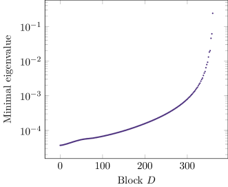
Figure 1. Minimal eigenvalue for each block $0\leq D\leq 360$, $N=120$.

The main computational task in the proof of the theorem is the numerical approximation of the various integrals $I_{\bf k}$. The number of such integrals increases as the fifth power of $N$; approximately $2.1\times 10^{5}$ distinct integrals (up to sign and permutation of ${\bf k}$) must be calculated for the $N=30$ case, increasing to approximately $1.6\times 10^{8}$ for the $N=120$ case. In Section 2, we describe carefully the numerical scheme used to approximate each ${I_{\bf k}}$ and estimate the associated error. This scheme is an improved version of the scheme given in [OTZ19], requiring fewer arithmetic operations per integral. We also discuss the adjustment of the parameters in the scheme for arbitrary $N$.

Due to the high level of precision required, the various calculations used in the proof were performed using arbitrary-precision arithmetic as implemented in the Arb numerical library [Joh17]; when used carefully, such arithmetic provides rigorous error bounds for the output of calculations. The calculation code was written in C++, employing hybrid parallelization through the use of both OpenMP and MPI. Computations were performed in parallel using 94 nodes of a modern compute cluster, requiring approximately 16 hours of wall time. Weights and points used for Gauss-Legendre quadrature were calculated using Mathematica [W19] to high precision and imported into the main calculation code by hand. The calculations can be reproduced using the code given in the supporting information; a copy of the output of this code, showing the approximated eigenvalues of the matrices (1), is also given. Some results (plots, etc.) outside the scope of the main proof were calculated by post-processing the calculated integrals ${\tilde{I}_{\bf k}}$ using standard numerical software, as the precision requirements are in context less stringent.

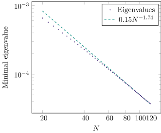
Figure 2. Minimal eigenvalues for the $D=0$ matrix in (1) with $20\leq N\leq 120$.

In Section 3, we describe the results of these computations, give an assessment of the eigenvalues, and discuss various plots of matrix entries and eigenfunctions. The quality of the experimentally-obtained information about the matrices in (1) and their eigenvalues and eigenfunctions has substantially improved compared to the computations in [OTZ19]. Phenomena are seen with much better resolution and allow further investigation. In particular, we obtain positivity of all eigenvalues in question, as shown to sufficient accuracy in Figure 1, which implies Theorem 1 by the reductions described in [OTZ19].​

Figure 1 shows that $D=0$ has the smallest eigenvalue among the matrices in (1) for $N=120$. It is cheap to conjecture that the analogous statement holds for arbitrarily large $N$. In addition, Figure 2 suggests the conjecture that the smallest eigenvalue of the matrix $D=0$ has a power decay, possibly of the order $N^{-7/4}$, and is in particular positive. These conjectures would imply the analogue to Theorem 1 for arbitrarily large $N$, and with it the general conjecture about constant functions maximizing the Tomas-Stein functional in $L^{2}\left\lparen\mathbb{S}^{1}\right\rparen$.

2. Numerical estimation of $I_{\bf k}$ and error bounds

As in [OTZ19], we approximate integrals $I_{\bf k}$ by quantities $\tilde{I}_{\bf k}$ defined by approximating schemes. We split

(2) $$\begin{split}I_{\bf k}&={I}^{0,S}_{\bf k}+{I}^{S,T}_{\bf k}+{I}^{T,\infty}_{\bf k}\\ &=\int_{0}^{S}\prod_{j=1}^{6}J_{k_{j}}\left\lparen r\right\rparen r\,\mathrm{d}r+\int_{S}^{T}\prod_{j=1}^{6}J_{k_{j}}\left\lparen r\right\rparen r\,\mathrm{d}r+\int_{T}^{\infty}\prod_{j=1}^{6}J_{k_{j}}\left\lparen r\right\rparen r\,\mathrm{d}r,\end{split}$$

and correspondingly combine

(3) $$\tilde{I}_{\bf k}=\tilde{I}^{0,S}_{\bf k}+\tilde{I}^{S,T}_{\bf k}+\tilde{I}^{T,\infty}_{\bf k},$$

where the first two terms are quadrature rules with different parameters approximating the corresponding compact integrals in (2), and the third term is an exact integral over an approximation to the integrand using asymptotic expansion. As opposed to [OTZ19], we use Gauss-Legendre quadrature instead of Newton-Cotes quadrature on the first two pieces, and we use more terms of the asymptotic expansion on the third integral. The cutoffs $S$ and $T$ should be chosen well for numerical speed and accuracy. Our discussion of the error bounds requires $S\geq 0.95N^{3/2}\ln\left\lparen N\right\rparen+1$ and $T>10N^{2}$. For $N=120$, in accordance with these conditions, we choose $S=6{,}000$ and $T=150{,}000$.

2.1. Gauss-Legendre quadrature on the intervals $\left[0,S\right]$ and $\left[S,T\right]$

We cut each of the intervals $\left[0,S\right]$ and $\left[S,T\right]$ into small intervals of constant length and use Gauss-Legendre quadrature with $n=12$ points on each of these small intervals. We will estimate the error of the quadrature using Lemma 3 below. We first quickly review the theory behind this lemma.

In $L^{2}\left\lparen\left[-1,1\right]\right\rparen$, the even or odd real monic polynomial

(4) $$\frac{n!}{\left\lparen 2n\right\rparen!}\partial_{x}^{n}{\left\lparen x^{2}-1\right\rparen}^{n}=\vcentcolon{}\prod_{i=1}^{n}\left\lparen x-x_{i}\right\rparen=\vcentcolon{}p_{n}\left\lparen x\right\rparen$$

is orthogonal to all polynomials of lower degree (this is the Rodrigues formula for the Legendre polynomials with a different constant factor). This is seen by $n$-fold partial integration, with boundary terms vanishing due to the structure of $p_{n}$. The zeroes $x_{1},\dots,x_{n}$ are distinct and contained in $\left\lparen-1,1\right\rparen$, or else there was a lower degree polynomial with the same sign as $p_{n}$ on $\left[-1,1\right]$, contradicting orthogonality. The linear combination $xp_{n}-p_{n+1}$ has degree at most $n$ and is orthogonal to all polynomials $p_{k}$ with $k<n-1$. By parity consideration, it is a multiple of $p_{n-1}$ with factor determined by examination of the highest order coefficient:

$$xp_{n}-p_{n+1} =\left[\frac{-n^{2}\left\lparen n-1\right\rparen}{\left\lparen 2n\right\rparen\left\lparen 2n-1\right\rparen}-\frac{-{\left\lparen n+1\right\rparen}^{2}n}{\left\lparen 2n+2\right\rparen\left\lparen 2n+1\right\rparen}\right]p_{n-1}$$

$$=\frac{n^{2}}{\left\lparen 2n+1\right\rparen\left\lparen 2n-1\right\rparen}p_{n-1}.$$

Pairing with $p_{n-1}$, using orthogonality relations, identifying the $n$-th factor of the Wallis product, and solving the recursion yields

$$\int_{-1}^{1}p_{n}^{2}\left\lparen x\right\rparen\,\mathrm{d}x=\frac{1}{4}\frac{{\left\lparen 2n\right\rparen}^{2}}{\left\lparen 2n-1\right\rparen\left\lparen 2n+1\right\rparen}\int_{-1}^{1}p_{n-1}^{2}\left\lparen x\right\rparen\,\mathrm{d}x\leq 2^{-2n}\pi.$$

Lemma 2 (Gauss-Legendre quadrature).

There are weights $w_{i}$ such that, for every function $f$ that is $2n$ times continuously differentiable on $\left[-1,1\right]$, we have

(5) $$\left\lvert\int_{-1}^{1}f\left\lparen y\right\rparen\,\mathrm{d}y-\sum_{i=1}^{n}w_{i}f\left\lparen x_{i}\right\rparen\right\rvert\leq\pi 2^{-2n}\sup_{\xi\in\left[-1,1\right]}\frac{\left\lvert f^{\left\lparen 2n\right\rparen}\left\lparen\xi\right\rparen\right\rvert}{\left\lparen 2n\right\rparen!}$$

Proof.

By regularity of the Vandermonde determinant, there are weights $w_{i}$ such that the left-hand-side of (5) vanishes if $f$ is a polynomial of degree at most $n-1$. The left-hand-side also vanishes evidently for all polynomials of the form $x^{k}p_{n}$ with $k\leq n-1$, and thus for all polynomials of degree at most $2n-1$. For arbitrary $f$ as in the lemma, let $h$ be the polynomial of degree $<2n$ such that $f-h$ vanishes of second order at all points $x_{i}$. Then the function $k=\left\lparen f-h\right\rparen p_{n}^{-2}$ is continuous. We estimate the left-hand-side of (5) as:

$$\int_{-1}^{1}\left\lparen f-h\right\rparen\left\lparen y\right\rparen\,\mathrm{d}y =\int_{-1}^{1}k\left\lparen y\right\rparen p_{n}{\left\lparen y\right\rparen}^{2}\,\mathrm{d}y$$

$$\leq\left\lvert k\left\lparen x\right\rparen\right\rvert\int_{-1}^{1}p_{n}{\left\lparen y\right\rparen}^{2}\,\mathrm{d}y$$

$$\leq\pi 2^{-2n}\left\lvert k\left\lparen x\right\rparen\right\rvert$$

for some $x\in\left[-1,1\right]$. By Rolle’s theorem, there is a $\xi\in\left[-1,1\right]$ with

$$0=\partial_{\xi}^{2n}(f-h-k\left\lparen x\right\rparen{p}_{n}^{2})\left\lparen\xi\right\rparen=f^{\left\lparen 2n\right\rparen}\left\lparen\xi\right\rparen-k\left\lparen x\right\rparen\left\lparen 2n\right\rparen!\qed$$

Lemma 3.

Assume $f$ is analytic on the union of balls of radius $1$ about each of the points of the interval $\left[a,b\right]$ and bounded by $F$ on this union. Then

$$\left\lvert\int_{a}^{b}f\left\lparen x\right\rparen\,\mathrm{d}x-\sum_{i=1}^{n}w_{i}\frac{b-a}{2}f\left\lparen\frac{a+b}{2}+\frac{b-a}{2}x_{i}\right\rparen\right\rvert\leq\pi 2^{-2n}{\left\lparen\frac{\left\lvert b-a\right\rvert}{2}\right\rparen}^{2n+1}F.$$

Proof.

This follows by translation and dilation of $f$ from the case $\left[a,b\right]=\left[-1,1\right]$ with balls of radius $1$ replaced by balls of radius $2/\left\lvert b-a\right\rvert$. The estimate in case $\left[-1,1\right]$ follows from Lemma 2 when estimating $\frac{f^{\left\lparen 2n\right\rparen}\left\lparen\xi\right\rparen}{2n!}$ with Cauchy’s integral formula as an average of the analytic function $f$ over the circle of radius $2/\left\lvert b-a\right\rvert$ about the point $\xi$.∎

On the interval $\left[0,S\right]$, we use the bound

$$\lvert J_{n}\left\lparen z\right\rparen\rvert\leq e^{\lvert\Im\left\lparen z\right\rparen\rvert}$$

on the strip $\Im\left\lparen z\right\rparen\leq 1$, obtained as reviewed in Section 2 of [OT17] from the integral representation

$$J_{n}\left\lparen z\right\rparen=\frac{1}{2\pi}\int_{0}^{2\pi}e^{iz\sin\left\lparen\theta\right\rparen}e^{in\theta}\,\mathrm{d}\theta.$$

Hence, the function

(6) $$f\left\lparen z\right\rparen=z\prod_{i=1}^{6}J_{n_{i}}\left\lparen z\right\rparen$$

is bounded in absolute value by $\left\lvert z\right\rvert e^{6}$ on this strip. Cutting the interval $\left[0,S\right]$ into $K$ intervals of length $2d=S/K$ and using Gauss-Legendre quadrature as in Lemma 3 on each interval gives

(7) $$\begin{split}\left\lvert I_{\bf k}^{0,S}-\tilde{I}_{\bf k}^{0,S}\right\rvert&=\left\lvert\int_{0}^{S}{f}\left\lparen z\right\rparen\,\mathrm{d}z-\sum_{j=0}^{K-1}d\sum_{i=1}^{n}{w}_{i}f(d\left\lparen 2j+1\right\rparen+dx_{i})\right\rvert\\ &\leq\pi 2^{-2n}d^{2n+1}e^{6}\sum_{j=0}^{K-1}(2d\left\lparen j+1\right\rparen+1)\\ &\leq\pi 2^{-2n-1}d^{2n}e^{6}\int_{0}^{S}\left\lparen x+2d+1\right\rparen\,\mathrm{d}x\\ &\leq\pi 2^{-2n-1}d^{2n}e^{6}{\left\lparen S+2d+1\right\rparen}^{2}\\ &\leq 0.000038\times{\left\lparen S+2d+1\right\rparen}^{2}d^{24}\\ &\leq 0.1\times 10^{-10}.\end{split}$$

Here we have used $n=12$ in the penultimate and $S=6{,}000$ and $d=0.25$ in the ultimate inequality. Note that this estimate does not depend on particular assumptions on $S$, and our parameters lead to an algorithm with $144{,}000$ evaluations of the integrand.

On the interval $\left[S,T\right]$, we recall from [OT17, Section 2] the following representation for $J_{n}$, which arises through the change of variables $t=\cos\left\lparen\theta\right\rparen$ from the Poisson integral:

$$J_{n}\left\lparen z\right\rparen=\frac{{\left\lparen z/2\right\rparen}^{n}}{\Gamma\left\lparen n+1/2\right\rparen\Gamma\left\lparen 1/2\right\rparen}\int_{-1}^{1}\cos\left\lparen zt\right\rparen{\left\lparen 1-t^{2}\right\rparen}^{n-1/2}\,\mathrm{d}t.$$

We split $J_{n}=\frac{1}{2}\left\lparen J_{n}^{+}+J_{n}^{-}\right\rparen$, where $J_{n}^{+}\left\lparen\overline{z}\right\rparen=\overline{J_{n}^{-}\left\lparen z\right\rparen}$ and

$$J_{n}^{+}\left\lparen z\right\rparen=\frac{{\left\lparen z/2\right\rparen}^{n}}{\Gamma\left\lparen n+1/2\right\rparen\Gamma\left\lparen 1/2\right\rparen}\int_{-1}^{1}e^{izt}{\left\lparen 1-t^{2}\right\rparen}^{n-1/2}\,\mathrm{d}t.$$

Indeed, $J_{n}=J_{n}^{+}$ due to symmetry of the weight. A change of the contour integral leads to

(8) $$J_{n}^{+}\left\lparen z\right\rparen=\frac{{\left\lparen 2\pi z\right\rparen}^{-1/2}}{\Gamma\left\lparen\nu+1\right\rparen}\int_{0}^{\infty}e^{-u}u^{\nu}\left[e^{-i\omega}{\left\lparen 1-\frac{iu}{2z}\right\rparen}^{\nu}+e^{i\omega}{\left\lparen 1+\frac{iu}{2z}\right\rparen}^{\nu}\right]\,\mathrm{d}u$$

with the abbreviations

$$\nu \vcentcolon=n-\frac{1}{2},$$

$$\omega \vcentcolon=z-\frac{\pi}{4}-\frac{n\pi}{2}.$$

We split further $J_{n}^{+}=\frac{1}{2}\left\lparen J_{n}^{++}+J_{n}^{+-}\right\rparen$ with $J_{n}^{+-}\left\lparen\overline{z}\right\rparen=\overline{J_{n}^{++}\left\lparen z\right\rparen}$ and

(9) $$J_{n}^{++}\left\lparen z\right\rparen={\left\lparen\frac{2}{\pi z}\right\rparen}^{1/2}\frac{e^{i\omega}}{\Gamma\left\lparen\nu+1\right\rparen}\int_{0}^{\infty}e^{-u}u^{\nu}{\left\lparen 1+\frac{iu}{2z}\right\rparen}^{\nu}\,\mathrm{d}u.$$

Lemma 4.

Assume $N\geq 20$ and $0\leq n\leq N$. Assume $\left\lvert\Re\left\lparen z\right\rparen\right\rvert>0.95N^{\frac{3}{2}}\ln\left\lparen N\right\rparen$ and $\left\lvert\Im\left\lparen z\right\rparen\right\rvert\leq 1$. Then

$$\left\lvert J_{n}^{++}\left\lparen z\right\rparen\right\rvert\leq 3.36\left\lvert z\right\rvert^{-1/2}.$$

The analogous estimate holds for $J_{n}^{+-}$, $J_{n}^{+}$, $J_{n}^{-}$, and $J_{n}$.

Proof.

We first estimate the part of the integral in (9) from $0$ to $2N\ln\left\lparen N\right\rparen$. We estimate in this range

$$\begin{split}\frac{1}{2}&\leq\left\lvert 1+\frac{iu}{2z}\right\rvert=\left\lvert 1+\frac{u\Im\left\lparen z\right\rparen}{2\left\lvert z\right\rvert^{2}}+i\frac{u\Re\left\lparen z\right\rparen}{2\left\lvert z\right\rvert^{2}}\right\rvert\\ &\leq\sqrt{{\left\lparen 1+\frac{1}{0.9N^{2}\ln\left\lparen N\right\rparen}\right\rparen}^{2}+\frac{1}{0.9N}}\\ &\leq 1+\frac{1}{N},\end{split}$$

where the lower bound by $\frac{1}{2}$ will only be used if $\nu$ is negative, that is $\nu=-1/2$. We obtain

$$\begin{split}\left\lvert\int_{0}^{2N\ln\left\lparen N\right\rparen}e^{-u}u^{\nu}{\left\lparen 1+\frac{iu}{2z}\right\rparen}^{\nu}\,\mathrm{d}u\right\rvert&\leq e\int_{0}^{\infty}e^{-u}u^{\nu}\,\mathrm{d}u\\ &=e\Gamma\left\lparen\nu+1\right\rparen.\end{split}$$

Turning to the part of the integral in (9) from $2N\ln\left\lparen N\right\rparen$ to $\infty$, we estimate

$$\left\lvert 1\pm\frac{iu}{2z}\right\rvert^{\nu}\leq{\left\lparen\frac{u}{N}\right\rparen}^{\nu+2}.$$

Hence we have

$$\left\lvert\int_{2N\ln\left\lparen N\right\rparen}^{\infty}e^{-u}u^{\nu}{\left\lparen 1+\frac{iu}{2z}\right\rparen}^{\nu}\right\rvert\,\mathrm{d}u\leq e^{-N\ln\left\lparen N\right\rparen}\int_{0}^{\infty}e^{-u/2}u^{\nu}{\left\lparen\frac{u}{N}\right\rparen}^{\nu+2}\,\mathrm{d}u$$

$$=N^{-{N}-\nu-2}2^{2\nu+3}\Gamma\left\lparen 2\nu+3\right\rparen\leq\frac{1}{100}\Gamma\left\lparen\nu+1\right\rparen.$$

With $\left\lvert e^{i\omega}\right\rvert\leq\cosh\left\lparen\left\lvert\Im z\right\rvert\right\rparen\leq\cosh\left\lparen 1\right\rparen$ it follows that

$$\left\lvert J_{n}^{+}\left\lparen z\right\rparen\right\rvert\leq{\left\lparen\frac{2}{\pi\left\lvert z\right\rvert}\right\rparen}^{1/2}\cosh\left\lparen 1\right\rparen\left\lparen\frac{1}{100}+e\right\rparen\leq 3.36\left\lvert z\right\rvert^{-1/2}.$$

The analogous estimates for the other variants of Bessel’s function are clear. ∎

With Lemma 4, we estimate the function (6) on the strip $\Im\left\lparen z\right\rparen\leq 1$ and $\Re\left\lparen z\right\rparen\geq 0.95N^{\frac{3}{2}}\ln\left\lparen N\right\rparen$ in absolute value by ${\left\lparen 3.36\right\rparen}^{6}\left\lvert z\right\rvert^{-2}$. Cutting the interval $\left[S,T\right]$ into $K$ intervals of length $2d=\left\lparen T-S\right\rparen/K$ and using Gauss-Legendre quadrature as in Lemma 3 on each interval, we obtain

(10) $$\begin{split}\left\lvert I_{\bf k}^{S,T}-\tilde{I}_{\bf k}^{S,T}\right\rvert&=\left\lvert\int_{S}^{T}{f}\left\lparen z\right\rparen\,\mathrm{d}z-\sum_{j=0}^{K-1}d\sum_{i=1}^{n}{w}_{i}f(S+d\left\lparen 2j+1\right\rparen+dx_{i})\right\rvert\\ &\leq\frac{\pi}{2^{2n}}d^{2n+1}{\left\lparen 3.36\right\rparen}^{6}\sum_{j=0}^{K-1}{\left\lparen S+2dj-1\right\rparen}^{-2}\\ &\leq\frac{\pi}{2^{2n+1}}d^{2n}{\left\lparen 3.36\right\rparen}^{6}\int_{S}^{T}{\left\lparen x-1-2d\right\rparen}^{-2}\,\mathrm{d}x\\ &\leq\pi 2^{-2n-1}d^{2n}{\left\lparen 3.36\right\rparen}^{6}{\left\lparen S-1-2d\right\rparen}^{-1}\\ &\leq 0.000135\times{\left\lparen S-1-2d\right\rparen}^{-1}d^{24}\\ &\leq 1.1\times 10^{-10}.\end{split}$$

Here we used $n=12$ in the penultimate and $S=6{,}000$ and $d=0.8$ in the ultimate inequality. The use of Lemma 4 here requires $S\geq 0.95N^{3/2}\ln\left\lparen N\right\rparen+1$, which is satisfied with $N=120$ and $S=6{,}000$. Assuming $T=150{,}000$, this amounts to $1{,}080{,}000$ evaluations of the integrand.

2.2. Asymptotic approximation on the interval $\left[T,\infty\right)$

We present a precise error bound for the classical asymptotic expansion of order four of Bessel functions, a slight refinement of the corresponding discussion in Section 2 of [OT17].

Lemma 5.

Assume $N\geq 20$ and $n\leq N$. Assume $z$ is real and $z>2N^{\frac{3}{2}}\ln\left\lparen N\right\rparen$. Then

(11) $$\begin{split}\left\lparen\frac{\pi z}{2}\right\rparen^{\frac{1}{2}}J_{n}^{++}\left\lparen z\right\rparen e^{-i\omega}&=1+i\frac{\Gamma\left\lparen\nu+2\right\rparen}{2\Gamma\left\lparen\nu\right\rparen z}-\frac{\Gamma\left\lparen\nu+3\right\rparen}{8\Gamma\left\lparen\nu-1\right\rparen z^{2}}\\ &\qquad{}-i\frac{\Gamma\left\lparen\nu+4\right\rparen}{48\Gamma\left\lparen\nu-2\right\rparen z^{3}}+R\end{split}$$

with

$$\left\lvert R\right\rvert\leq 0.0043\frac{N^{8}}{z^{4}}.$$

Proof.

Recalling (9), we see

(12) $${\left\lparen\frac{\pi z}{2}\right\rparen}^{\frac{1}{2}}J_{n}^{++}\left\lparen z\right\rparen e^{-i\omega}=\frac{1}{\Gamma\left\lparen\nu+1\right\rparen}\int_{0}^{\infty}e^{-u}u^{\nu}{\left\lparen 1+\frac{iu}{2z}\right\rparen}^{\nu}\,\mathrm{d}u.$$

We expand ${\left\lparen 1+ix\right\rparen}^{\nu}$ for real $0\leq x$ with Taylor’s theorem into

$${\left\lparen 1+ix\right\rparen}^{\nu}=1+i\nu x-\frac{1}{2}\nu\left\lparen\nu-1\right\rparen x^{2}-\frac{1}{6}i\nu\left\lparen\nu-1\right\rparen\left\lparen\nu-2\right\rparen x^{3}+r$$

where

$$\left\lvert r\right\rvert =\left\lvert\int_{0}^{x}\frac{1}{6}\nu\left\lparen\nu-1\right\rparen\left\lparen\nu-2\right\rparen\left\lparen\nu-3\right\rparen{\left\lparen x-t\right\rparen}^{3}{\left\lparen 1+it\right\rparen}^{\nu-4}\,\,\mathrm{d}t\right\rvert$$

$$\leq\frac{1}{24}\left\lvert\nu\left\lparen\nu-1\right\rparen\left\lparen\nu-2\right\rparen\left\lparen\nu-3\right\rparen\right\rvert x^{4}{\left\lparen 1+x^{2}\right\rparen}^{\frac{1}{2}\max\left\{\nu-4,0\right\}}.$$

Thus the right hand side of (12) becomes (11) with

$$\left\lvert R\right\rvert\leq\int_{0}^{\infty}e^{-u}u^{\nu}\left\lvert r\left\lparen u\right\rparen\right\rvert\,\mathrm{d}u$$

and $r\left\lparen u\right\rparen$ similar to above with $x$ replaced by $u/2z$. We cut the integral at $u=4N\ln\left\lparen N\right\rparen$. For $u\leq 4N\ln\left\lparen N\right\rparen$ we have

$$\left\lvert r\left\lparen u\right\rparen\right\rvert\leq\frac{\lvert\nu\left\lparen\nu-1\right\rparen\left\lparen\nu-2\right\rparen\left\lparen\nu-3\right\rparen\rvert u^{4}}{384z^{4}}{\left\lparen 1+\frac{1}{N}\right\rparen}^{\frac{N}{2}}$$

and thus

$$\frac{1}{\Gamma\left\lparen\nu+1\right\rparen}\int_{0}^{4N\ln\left\lparen N\right\rparen}e^{u}u^{\nu}r\left\lparen u\right\rparen\,\mathrm{d}u\leq e^{1/2}\frac{\Gamma\left\lparen\nu+5\right\rparen}{384\lvert\Gamma\left\lparen\nu-3\right\rparen\rvert z^{4}}\leq\frac{e^{1/2}N^{8}}{384z^{4}}.$$

For $u\geq 4N\ln\left\lparen N\right\rparen$ we have

$$\left\lvert r\left\lparen u\right\rparen\right\rvert\leq\frac{\lvert\nu\left\lparen\nu-1\right\rparen\left\lparen\nu-2\right\rparen\left\lparen\nu-3\right\rparen\rvert u^{4}}{6{\left\lparen 2z\right\rparen}^{4}}{\left\lparen\frac{u}{N}\right\rparen}^{N/2},$$

and therefore

$$\frac{1}{\Gamma\left\lparen\nu+1\right\rparen}\int_{4N\ln\left\lparen N\right\rparen}^{\infty}e^{-u}u^{\nu}r\left\lparen u\right\rparen\,\mathrm{d}u$$

$$\leq\frac{1}{384z^{4}\lvert\Gamma\left\lparen\nu-3\right\rparen\rvert}\int_{0}^{\infty}e^{-u/2}e^{-2N\ln\left\lparen N\right\rparen}u^{\nu+4}{\left\lparen\frac{u}{N}\right\rparen}^{N/2}\,\mathrm{d}u$$

$$\leq\frac{1}{96z^{4}\lvert\Gamma\left\lparen\nu-3\right\rparen\rvert}\frac{2^{\nu+5+N/2}}{N^{2N+N/2}}\Gamma\left\lparen\nu+5+N/2\right\rparen\leq z^{-4}.$$

Adding the estimates for the two pieces of the integral gives the bound claimed in the lemma. ∎

With the above lemma, we obtain for $J^{+}_{n}$ in the range of $n$ and $z$ discussed in the lemma:

(13) $${\left\lparen\frac{\pi z}{2}\right\rparen}^{\frac{1}{2}}J_{n}^{+}\left\lparen z\right\rparen=a+bz^{-1}+cz^{-2}+dz^{-3}+R$$

with

$$a =\cos\left\lparen\omega\right\rparen,$$

$$b =-\sin\left\lparen\omega\right\rparen\frac{1}{2}\left\lparen n^{2}-\frac{1}{4}\right\rparen,$$

$$c =-\cos\left\lparen\omega\right\rparen\frac{1}{8}\left\lparen n^{2}-\frac{1}{4}\right\rparen\left\lparen n^{2}-\frac{9}{4}\right\rparen,$$

$$d =\sin\left\lparen\omega\right\rparen\frac{1}{48}\left\lparen n^{2}-\frac{1}{4}\right\rparen\left\lparen n^{2}-\frac{9}{4}\right\rparen\left\lparen n^{2}-\frac{25}{4}\right\rparen,$$

and $R$ satisfies the same bounds as in the lemma. The analogous identity holds for $J_{n}$ since it coincides with $J_{n}^{+}$ on the real line. Now we consider six indices $n_{j}$ and corresponding $\omega_{j}\vcentcolon=z-\pi/4-n_{j}\pi/2$ and obtain for real $z$

$${\left\lparen\frac{\pi}{2}\right\rparen}^{3}\prod_{j=1}^{6}J_{n_{j}}\left\lparen z\right\rparen z=Az^{-2}+Bz^{-3}+Cz^{-4}+Q$$

with

$$A =\cos\left\lparen\omega_{1}\right\rparen\cos\left\lparen\omega_{2}\right\rparen\cos\left\lparen\omega_{3}\right\rparen\cos\left\lparen\omega_{4}\right\rparen\cos\left\lparen\omega_{5}\right\rparen\cos\left\lparen\omega_{6}\right\rparen,$$

$$B =-\sum_{j^{\prime}=1}^{6}\frac{n_{j^{\prime}}^{2}-1/4}{2}\sin\left\lparen\omega_{j^{\prime}}\right\rparen\prod_{1\leq j\leq 6,j\neq j^{\prime}}\cos\left\lparen\omega_{j}\right\rparen,$$

$$C =\sum_{j^{\prime}=1}^{6}\sum_{j^{\prime\prime}=j^{\prime}+1}^{6}\frac{\left\lparen n_{j^{\prime}}^{2}-1/4\right\rparen\left\lparen n_{j^{\prime\prime}}^{2}-1/4\right\rparen}{4}\sin\left\lparen\omega_{j^{\prime}}\right\rparen\sin\left\lparen\omega_{j^{\prime\prime}}\right\rparen\prod_{1\leq j\leq 6,j\neq j^{\prime},j\neq j^{\prime\prime}}\cos\left\lparen\omega_{j}\right\rparen$$

$$\qquad{}-\frac{\left[\sum_{j=1}^{6}\left\lparen n_{j}^{2}-1/4\right\rparen\left\lparen n_{j}^{2}-9/4\right\rparen\right]}{8}\prod_{j=1}^{6}\cos\left\lparen\omega_{j}\right\rparen.$$

The remainder term $Q$ we estimate from above. For this we collect terms of order $z^{-5}$, $z^{-6}$, $z^{-7}$, $z^{-8}$ and higher order separately. We begin with a remark on integrals of type

$$\int_{T}^{\infty}\prod_{j=1}^{6}\phi_{j}\left\lparen\omega_{j}\right\rparen z^{-5}$$

where an odd number of functions $\phi_{j}$ are the cosine function and an odd number of $\phi_{j}$ are the sine function. If a function is odd in the variable $z$ about the point $\frac{\pi}{4}$ then we call it of parity $-1$, and if it is even we call it of parity $1$. The function

$$\sin\left\lparen\omega_{j}\right\rparen=\sin\left\lparen z-\frac{\pi}{4}-\frac{n\pi}{2}\right\rparen$$

has parity $-{\left\lparen-1\right\rparen}^{n}$ about the point $\frac{\pi}{4}$, while the function

$$\cos\left\lparen\omega_{j}\right\rparen=\cos\left\lparen z-\frac{\pi}{4}-\frac{n\pi}{2}\right\rparen$$

has parity ${\left\lparen-1\right\rparen}^{n}$. A product of six such functions with $\sum_{j=1}^{6}n_{j}$ even and an involving an odd number of sine function is therefore odd about the point $\pi/4$. This means it integrates to zero about each period of the periodic function. Hence by partial integration

$$\left\lvert\int_{T}^{\infty}\prod_{j=1}^{6}\phi_{j}\left\lparen\omega_{j}\right\rparen z^{-5}\,\mathrm{d}z\right\rvert \leq\left\lvert\int_{T}^{\infty}\partial_{z}^{-1}\left[\prod_{j=1}^{6}\phi_{j}\left\lparen\omega_{j}\right\rparen\right]5z^{-6}\,\mathrm{d}z\right\rvert+T^{-5}$$

$$\leq\left\lparen\pi+1\right\rparen T^{-5}$$

where we used that the function $\prod_{j=1}^{6}\phi_{j}\left\lparen\omega_{j}\right\rparen$ is bounded by $1$ and since it integrates to $0$ of periods of length $2\pi$ its primitive $\partial_{z}^{-1}\left[\prod_{j=1}^{6}\phi_{j}\left\lparen\omega_{j}\right\rparen\right]$ is bounded by $\pi$.

We use this estimate in each of the terms of the fifth order, all of which have an odd number of sine functions. We estimate all factors $n_{j}^{2}-x$ by $N^{2}$. Counting the terms and referring to the abbreviations in (13), we obtain $6$ terms with a factor $d$, $30$ factors with a product $bc$ and $20$ terms with a factor $b^{3}$. Thus this term is estimated by

(14) $$\left\lparen\frac{6}{48}+\frac{30}{16}+\frac{20}{8}\right\rparen\left\lparen 1+\pi\right\rparen\frac{N^{6}}{T^{5}}\leq 19\frac{N^{6}}{T^{5}}.$$

To estimate sixth order terms we estimate all sine and cosine functions by $1$. Integrating $z^{-6}$ then simply gives $T^{-5}/5$. We obtain $6$ terms with a factor $R$, $30$ terms with a factor $bd$, $15$ terms with a factor $c^{2}$, $60$ terms with a factor $cb^{2}$, $15$ terms with a factor $b^{4}$. This gives the estimate

(15) $$\left\lparen 6\times 0.0043+\frac{30}{96}+\frac{15}{64}+\frac{60}{32}+\frac{15}{16}\right\rparen\frac{N^{8}}{5T^{5}}\leq 0.68\frac{N^{8}}{T^{5}}.$$

The seventh order terms we estimate similarly. We obtain $30$ terms with a factor $Rb$, $30$ terms with a factor $dc$, $60$ terms with a factor $db^{2}$, $60$ terms with a factor $c^{2}b$, $60$ terms with a factor $cb^{3}$ and $6$ terms with a factor $b^{5}$. This gives the estimate

(16) $$\left\lparen\frac{30}{2}\times 0.0043+\frac{30}{384}+\frac{60}{192}+\frac{60}{128}+\frac{60}{64}+\frac{6}{32}\right\rparen\frac{N^{10}}{6T^{6}}\leq 0.35\frac{N^{10}}{T^{6}}.$$

Counting the eighth order terms we find $30$ terms with a factor $Rc$, $60$ terms with a factor $Rb^{2}$, $15$ terms with a factor $d^{2}$, $120$ terms with a factor $dcb$, $60$ terms with a factor $db^{3}$, $15$ terms with a factor $c^{3}$, $45$ terms with a factor $c^{2}b^{2}$, $30$ terms with a factor $cb^{4}$, and one term with a factor $b^{6}$. This gives the estimate

(17) $$\begin{split}\left\lparen\vphantom{0.0043\left\lparen\frac{30}{8}+\frac{60}{4}\right\rparen+\frac{15}{2304}+\frac{120}{768}+\frac{60}{384}+\frac{15}{512}+\frac{45}{256}+\frac{30}{128}+\frac{1}{32}}0.0043\left\lparen\frac{30}{8}+\frac{60}{4}\right\rparen\right.&+\frac{15}{2304}+\frac{120}{768}+\frac{60}{384}\\ &\left.\vphantom{0.0043\left\lparen\frac{30}{8}+\frac{60}{4}\right\rparen+\frac{15}{2304}+\frac{120}{768}+\frac{60}{384}+\frac{15}{512}+\frac{45}{256}+\frac{30}{128}+\frac{1}{32}}+\frac{15}{512}+\frac{45}{256}+\frac{30}{128}+\frac{1}{32}\right\rparen\frac{N^{12}}{7T^{7}}\leq 0.13\frac{N^{12}}{T^{7}}.\end{split}$$

The terms of order $9$ or higher we estimate more crudely. There are at most $5^{6}$ terms, the product of pre factors being at most $0.0043$ if a factor $R$ is involved and being at most $\frac{1}{128}$ if no such factor is involved. Thus we get, assuming $N^{2}\leq T$, the upper bound

(18) $$\leq\frac{5^{6}}{128}\frac{N^{14}}{8T^{8}}\leq 16\frac{N^{14}}{T^{8}}.$$

Assuming $N=120\geq 20$ and $T\geq 10N^{2}$ we may add (14), (15), (16), (17), and (18) to

(19) $$\begin{split}\left\lvert I_{\bf k}^{T,\infty}-\tilde{I}_{\bf k}^{T,\infty}\right\rvert&\leq\left\lparen\vphantom{19\times 10^{-4}20^{-2}+0.68\times 10^{-4}+0.35\times 10^{-5}+0.13\times 10^{-6}+16\times 10^{-7}}19\times 10^{-4}20^{-2}+0.68\times 10^{-4}+0.35\times 10^{-5}\right.\\ &\qquad\left.\vphantom{19\times 10^{-4}20^{-2}+0.68\times 10^{-4}+0.35\times 10^{-5}+0.13\times 10^{-6}+16\times 10^{-7}}+0.13\times 10^{-6}+16\times 10^{-7}\right\rparen{}T^{-1}\\ &\leq 0.75\times 10^{-4}T^{-1}\\ &\leq 0.5\times 10^{-9}.\end{split}$$

Here we used $T=150{,}000>10N^{2}$ in the last inequality. Summing (7), (10), and (19), we finally obtain

(20) $$\left\lvert I_{\bf k}-\tilde{I}_{\bf k}\right\rvert\leq 0.73\times 10^{-9}.$$

3. Numerical Results

Using the approximations $\tilde{I}_{\bf k}$, one computes approximations ${\lparen\tilde{Q}_{{\bf m},{\bf n}}\rparen}_{{\bf m},{\bf n}\in{X}_{D}}$ to the matrices ${\lparen Q_{{\bf m},{\bf n}}\rparen}_{{\bf m},{\bf n}\in{X}_{D}}$ analogously to the formulae in the introduction. Using evaluations of Bessel functions of sufficient accuracy and arbitrary-precision arithmetic, the $\tilde{I}_{\bf k}$ and $\tilde{Q}_{{\bf m},{\bf n}}$ as well as the eigenvalues of the matrices ${\lparen\tilde{Q}_{{\bf m},{\bf n}}\rparen}_{{\bf m},{\bf n}\in{X}_{D}}$ were computed up to an error of at most $10^{-20}$. The computed smallest eigenvalue for each $D$ is plotted in Figure 1 and shown in Table 1 for small $D$. In particular, the matrix ${\lparen\tilde{Q}_{{\bf m},{\bf n}}\rparen}_{{\bf m},{\bf n}\in{X}_{D}}$ is positive definite with smallest eigenvalue at least $0.000036$.

$D$	$\lambda_{\min}$
0	0.0000369980
2	0.0000371564
4	0.0000374854
6	0.0000379002
8	0.0000384081
10	0.0000389622

Table 1. Smallest eigenvalues for matrices ${\left\lparen Q_{{\bf m},{\bf n}}\right\rparen}_{{\bf m},{\bf n}\in X_{D}}$, for $D=0,2,\ldots,10$, rounded to 11 significant figures.

We have for each ${\bf m},{\bf n}$ in question from (20)

$$\left\lvert{Q}_{{\bf m},{\bf n}}-\tilde{Q}_{{\bf m},{\bf n}}\right\rvert\leq 16\times 0.73\times 10^{-9}\leq 1.2\times 10^{-8}.$$

This entry-wise bound is multiplied by the size $1860$ of the set $X_{D}$ for $N=120$ to obtain a bound for the operator norm

$$\left\lVert{\left\lparen{Q}_{{\bf m},{\bf n}}\right\rparen}_{{\bf m},{\bf n}\in{X}_{D}}-{\left\lparen\tilde{Q}_{{\bf m},{\bf n}}\right\rparen}_{{\bf m},{\bf n}\in{X}_{D}}\right\rVert_{op}\leq 1860\times 1.2\times 10^{-8}\leq 0.000023.$$

As this is less than the smallest eigenvalue of the matrix

$${\left\lparen\tilde{Q}_{{\bf m},{\bf n}}\right\rparen}_{{\bf m},{\bf n}\in{X}_{D}},$$

we may deduce that the matrix ${\lparen{Q}_{{\bf m},{\bf n}}\rparen}_{{\bf m},{\bf n}\in{X}_{D}}$ is positive definite as well. Following the reductions of [OTZ19], this proves Theorem 1.

While the error bounds (20) are good enough to prove the main theorem, they are not good enough to guarantee that our plots and tables of eigenvalues of ${\lparen\tilde{Q}_{{\bf m},{\bf n}}\rparen}_{{\bf m},{\bf n}\in{X}_{D}}$ are representative for those of ${\lparen{Q}_{{\bf m},{\bf n}}\rparen}_{{\bf m},{\bf n}\in{X}_{D}}$ within the margins suggested by the visible information. However, the arguments obtaining (20) as well as the use of the operator norm above are very crude estimates. With very high likelihood, the true differences between the corresponding eigenvalues of the two matrices are much smaller than the operator norm above. In this sense, we consider our plots and tables of eigenvalues of ${\lparen\tilde{Q}_{{\bf m},{\bf n}}\rparen}_{{\bf m},{\bf n}\in{X}_{D}}$ as very much representative of those of ${\lparen{Q}_{{\bf m},{\bf n}}\rparen}_{{\bf m},{\bf n}\in{X}_{D}}$. This is in accordance with the rather regular behaviour of the plots and of Table 1, a level of regularity that one might expect from the eigenvalues of ${\lparen{Q}_{{\bf m},{\bf n}}\rparen}_{{\bf m},{\bf n}\in{X}_{D}}$.

A number of numerical findings would be interesting to understand analytically and maybe prove for large $N$ asymptotically. Any progress in this understanding would presumably require an asymptotic understanding of the entries of the matrices in (1). Figure 3 shows sample columns of these matrices. For nicer visualization, we have undone the dimension reduction by symmetry in [OTZ19] and shown the related matrices

(21) $$\tilde{Q}^{\left\lparen D\right\rparen}\vcentcolon={\left\lparen Q_{{\bf m},{\bf n}}\right\rparen}_{{\bf m},{\bf n}\in Z_{D}},$$

in the space

$$Z_{D}\vcentcolon=\left\{\left\lparen m_{1},m_{2},m_{3}\right\rparen\in{\left\lparen 2\mathbb{Z}\right\rparen}^{3}\setminus\{\left\lparen 0,0,0\right\rparen\}\nonscript\>\middle|{}\allowbreak{}\nonscript\>\mathopen{}\begin{subarray}{c}m_{1}+m_{2}+m_{3}=D,\\ \left\lvert m_{1}\right\rvert,\left\lvert m_{2}\right\rvert,\left\lvert m_{3}\right\rvert\leq N\end{subarray}\right\}.$$

The space $Z_{D}$ is naturally depicted as a hexagon. It has a sixfold symmetry under permutations of the three elements, which is the symmetry group of a regular hexagon. This symmetry extends to symmetries of the columns shown and is visible in the plots of Figure 3. The space $X_{D}$ in our previous calculations is only one fundamental domain under this symmetry.

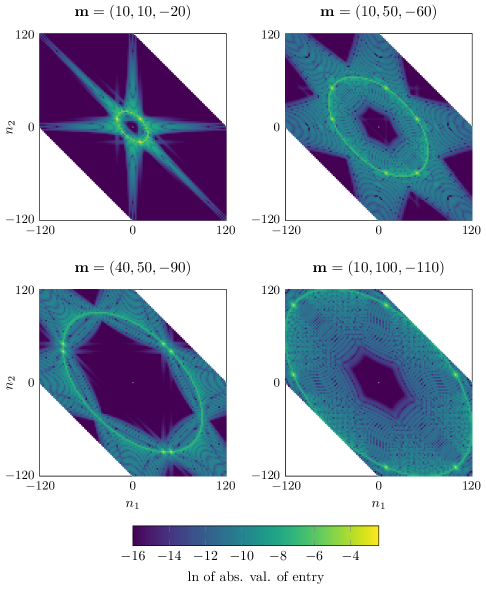
Figure 3. Columns of (21) with $D=0$ and $N=120$ for sample fixed values of ${\bf m}$, in coordinates $n_{1},n_{2}$. Coloring is logarithmic in the absolute values of entries; logarithmic values below $-16$ are clipped.

The largest entry in each column of the matrices in $\eqref{qmatrices}$ is the diagonal element. The diagonal elements appear as brights dots on the ellipses in Figure 3. Due to the sixfold symmetry of the visualization, they appear three or six times in each image depending on their orbit under the symmetry group, namely the points where $\mathbf{m}$ is a permutation of $\mathbf{n}$. While it may be tempting to try to prove positive definiteness of the matrices in (1) by diagonal dominance, for $N=120$ and $D=0$, the ratios

(22) $$r_{\mathbf{m}}\vcentcolon=\lvert Q_{\bf{m},\bf{m}}\rvert^{-1}\sum_{\mathbf{n}\in X_{0}\setminus\{\mathbf{m}\}}\lvert Q_{\bf{m},\bf{n}}\rvert,$$

can be large as well as small, e.g.

$$r_{\left\lparen-2,0,2\right\rparen}\approx 3.1,\quad r_{\left\lparen-90,40,50\right\rparen}\approx 1.9,\quad r_{\left\lparen-4,2,2\right\rparen}\approx 0.7.$$

Indeed, this failure of this attempt is natural due to the existence of some very small eigenvalues.

A secondary collection of large entries in each column shown in Figure 3 can be seen as yellow ellipses in the diagrams. These visual ellipses correspond to circles in a visualization of the domain as regular hexagon. The circles were already observed in [OTZ19]. The current data even more strongly suggests that these secondary peaks are located on the surface

(23) $$n_{1}^{2}+n_{2}^{2}+n_{3}^{2}=m_{1}^{2}+m_{2}^{2}+m_{3}^{2}.$$

Indeed, in Figure 4, the ellipse/circle given by (23), plotted as a white line, is overlayed onto one of the plots, showing that it matches the yellow peaks very well. The size of the sum of off-diagonal elements in (22) is essentially entirely due to the elements near the circle.

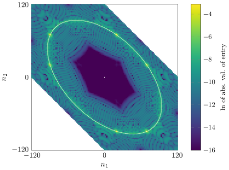
Figure 4. Column ${\bf m}=\left\lparen 20,70,-90\right\rparen$ of (21) with $D=0$ and $N=120$, in coordinates $n_{1},n_{2}$. Coloring is logarithmic in the absolute values of entries; logarithmic values below $-16$ are clipped. The white line indicates the ellipse given by (23).

At the moment, we do not even have a qualititive understanding of the occurrence of these circles, let alone a quantitative one, which would probably be required if one wanted to extract positive definiteness from the structure of these matrices. Figure 5 plots the values of the entries of the column $\left\lparen 40,60,-100\right\rparen$ as a function of the radial variable $\sqrt{n_{1}^{2}+n_{2}^{2}+n_{3}^{2}}$ in the vicinity of the radius of the yellow circle, which is about $123.3$. The plot strongly suggests that the pattern of the circle is asymptotically well approximated by a smooth radial function of low complexity. The value at the diagonal element, which is at radius about $123.3$, is not plotted in Figure 5, because it is too large at about $0.044$. Likewise, two further entries near the diagonal elements are not shown, they have value $-0.0024$. They are part of the small ring of six large elements around the diagonal elements, which also include the four entries with values near $-0.0015$ shown in Figure 5. Also, small matrix entries are cut off in the plot 5.

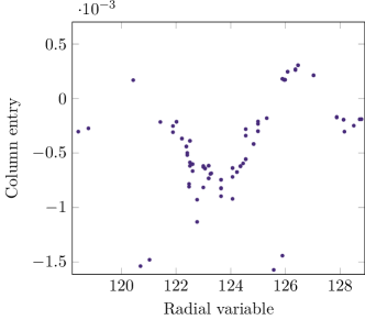
Figure 5. Partial plot of the values of the entries of column ${\bf m}=\left\lparen 40,60,-100\right\rparen$ of (21) with $D=0$ and $N=120$ in dependence of the radial variable.

Due to the monotonicity shown in Figure 1, it is of particular interest to study the matrix in (1) for $D=0$. Figure 6 shows all eigenvalues of the matrix $D=0$ for $N=120$ sorted and enumerated by size. For comparison, we also show the analogous plot for the matrix $D=200$, a diagram that is somewhat similar. Note the two jumps of the diagram for $D=0$ at about the $60$-th smallest and $60$-th largest eigenvalues. An analytical proof of positivity for all $N$ in the asymptotic regime would require a better understanding of the ensemble of small eigenvalues below the first jump.

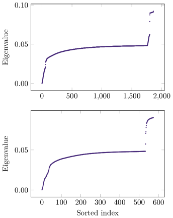
Figure 6. Sorted eigenvalues of 1 with $D=0$ (top, 1860 eigenvalues) and $D=200$ (bottom, 574 eigenvalues), both with $N=120$.

The eigenfunctions corresponding to the smallest eigenvalues experimentally appear to be essentially radial functions in the visualization corresponding to Figure 3, cf. Figure 7. There are three notable observations to be made here:

1. The bulk of the eigenvector depends essentially only on $\sqrt{n_{1}^{2}+n_{2}^{2}+n_{3}^{2}}$.

2. The value at the points where two of the $n_{i}$s coincide is smaller than suggested by this radial dependence by a factor of two (although this is not evident from this particular visualization).

3. Outside of the largest circle that fits into the region $Z_{0}$, the eigenvector is small.

The second point above is related to the fact that in the matrices (21), the rows and the columns of (21) appear as many times as there are distinct permutations of $\mathbf{m}$ and $\mathbf{n}$ respectively, i.e. 3 and 6 times. It therefore appears more natural to analyze the eigenvalues of (21), or, equivalently, the matrices given by ${\left\lparen p_{\mathbf{m}}Q_{\mathbf{m},\mathbf{n}}p_{\mathbf{n}}\right\rparen}_{\mathbf{m},\mathbf{n}\in X_{0}}$, where $p_{\mathbf{m}}$ is the number of distinct permutations of $\mathbf{m}$.

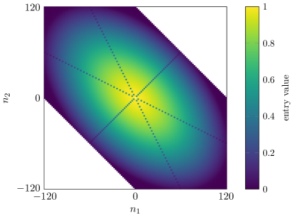
Figure 7. Eigenvector of (1) with $D=0$ and $N=120$ corresponding to the smallest eigenvalue in coordinates $n_{1},n_{2}$. The dotted lines are points where the orbit of the symmetry group has only three elements. They are an artifact of dimension reduction: the values of the eigenvector at these points are half as large as those of the corresponding eigenvector of (1).

In view of the third point above, it also appears natural to truncate the matrices not according to $\max\left\lparen\lvert n_{1}\rvert,\lvert n_{2}\rvert,\lvert n_{3}\rvert\right\rparen$, but according to $\sqrt{n_{1}^{2}+n_{2}^{2}+n_{3}^{2}}$. In what follows, let us therefore consider the matrices

(24) $$Q^{\circ}\vcentcolon=\left\lparen p_{\mathbf{m}}Q_{\mathbf{m},\mathbf{n}}p_{\mathbf{n}}\right\rparen_{\mathbf{m},\mathbf{n}\in X^{\circ}},$$

where

$$X^{\circ}=\left\{\left\lparen m_{1},m_{2},m_{3}\right\rparen\in{\left\lparen 2\mathbb{Z}\right\rparen}^{3}\setminus\{\left\lparen 0,0,0\right\rparen\}\nonscript\>\middle|{}\allowbreak{}\nonscript\>\mathopen{}\begin{subarray}{c}m_{1}+m_{2}+m_{3}=0,\\ \sqrt{m_{1}^{2}+m_{2}^{2}+m_{3}^{2}}\leq\sqrt{3/2}N,\\ m_{1}\leq m_{2}\leq m_{3}\end{subarray}\right\}.$$

is the largest disc contained in $X_{0}$. The eigenvectors of the matrices (24) corresponding to small eigenvalues seem to be smooth functions of the radial variable $\sqrt{n_{1}^{2}+n_{2}^{2}+n_{3}^{2}}$, see Figure 8. In that figure, the five smallest eigenvalues are represented by different colors. For each eigenvalue, there is a point for every $\mathbf{n}\in X^{\circ}$. Surprisingly, the corresponding eigenvector entries $s_{\bf{n}}$ fall on a one-dimensional curve, although $X^{\circ}$ is taken from a two-dimensional lattice. After a suitable rescaling, the profile of the curve seems to be independent of $N$, as shown in Figure 9 for the smallest eigenvalue.

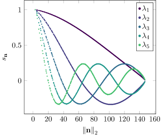
Figure 8. Eigenfunctions associated to five smallest eigenvalues $\lambda_{i},1\leq i\leq 5$ of (24) with $D=0$ and $N=120$.

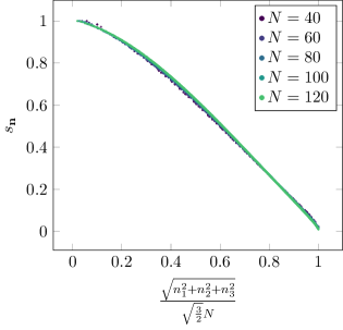
Figure 9. Eigenfunctions associated to the smallest eigenvalues of (24) with $D=0$ and $N\in\{40,60,80,100,120\}$.

It is natural to link the behaviour of the eigenfunctions to the smallest eigenvectors to a natural enemy of the sharp Fourier extension conjecture. Namely, functions on the circle which approximate two Dirac deltas at antipodally symmetric points are close competitors to extremize the Tomas-Stein functional; they “lose” to the constant function by only a small amount. Such Dirac deltas, on the Fourier transform side depicted in the above hexagons, correspond to wide bumps such as the lowest eigenfunction. One can well imagine that all the radial eigenfunctions to small eigenvalues aspire to resolve structure near the Dirac deltas.

References

- [Car+17] Emanuel Carneiro, Damiano Foschi, Diogo Oliveira e Silva and Christoph Thiele “A sharp trilinear inequality related to Fourier restriction on the circle” In Rev. Mat. Iberoam. 33.4, 2017, pp. 1463–1486 DOI: 10.4171/RMI/978
- [FO17] Damiano Foschi and Diogo Oliveira e Silva “Some recent progress on sharp Fourier restriction theory” In Anal. Math. 43.2, 2017, pp. 241–265 DOI: 10.1007/s10476-017-0306-2
- [Joh17] Fredrik Johansson “Arb: efficient arbitrary-precision midpoint-radius interval arithmetic” In IEEE Transactions on Computers 66.8 IEEE, 2017, pp. 1281–1292
- [OT17] Diogo Oliveira e Silva and Christoph Thiele “Estimates for certain integrals of products of six Bessel functions” In Rev. Mat. Iberoam. 33.4, 2017, pp. 1423–1462 DOI: 10.4171/RMI/977
- [OTZ19] Diogo Oliveira e Silva, Christoph Thiele and Pavel Zorin-Kranich “Band-limited maximizers for a Fourier extension inequality on the circle” In Experimental Mathematics Taylor & Francis, 2019, pp. 1–7 arXiv:1806.06605
- [Tom75] Peter A. Tomas “A restriction theorem for the Fourier transform” In Bull. Amer. Math. Soc 81.2, 1975, pp. 477–478
- [W19] Wolfram Research Inc. “Mathematica, Version 12.0” Champaign, IL, 2019 URL: https://www.wolfram.com/mathematica