How dynamics constrains probabilities in general probabilistic theories
Abstract
We introduce a general framework for analysing general probabilistic theories, which emphasises the distinction between the dynamical and probabilistic structures of a system. The dynamical structure is the set of pure states together with the action of the reversible dynamics, whilst the probabilistic structure determines the measurements and the outcome probabilities. For transitive dynamical structures whose dynamical group and stabiliser subgroup form a Gelfand pair we show that all probabilistic structures are rigid (cannot be infinitesimally deformed) and are in one-to-one correspondence with the spherical representations of the dynamical group. We apply our methods to classify all probabilistic structures when the dynamical structure is that of complex Grassmann manifolds acted on by the unitary group. This is a generalisation of quantum theory where the pure states, instead of being represented by one-dimensional subspaces of a complex vector space, are represented by subspaces of a fixed dimension larger than one. We also show that systems with compact two-point homogeneous dynamical structures (i.e. every pair of pure states with a given distance can be reversibly transformed to any other pair of pure states with the same distance), which include systems corresponding to Euclidean Jordan Algebras, all have rigid probabilistic structures.
1 Introduction
General probabilistic theories (GPTs) provide a framework for the study of operational theories beyond quantum theory. Within this framework quantum theory appears as one non-classical theory amongst many. This field has its origin in the work of Segal [1], Mackey [2] and Ludwig [3, 4, 5] with other notable contributions at the time including [6, 7, 8, 9, 10, 11, 12, 13] amongst others. Contemporary interest in GPTs was kickstarted by Hardy’s seminal work [14] followed by a detailed exposition of the framework by Barrett [15]. Important applications of the framework include the operational derivations of quantum theory of [16, 17, 18]. Current treatments have tended to emphasise finite dimensional systems and system composition. Using this framework (or related frameworks such as convex operational theories [19, 20] and operational probabilistic theories [21]) many physical and informational features of general probabilistic theories have been studied, such as interference phenomena [22, 23, 24, 25], computation [26, 27], thermodynamics [28, 29, 30] and others [31, 32, 33, 34, 35, 36, 37, 38].
Examples of GPTs (excepting classical and quantum theory) include Boxworld [39, 15, 40, 41, 42], quantum theory over the field of real numbers [43, 44, 45] or quaternions [46], theories based on Euclidean Jordan algebras [35], quartic quantum theory [47], -balls [16, 48, 49], density cubes [50] and quantum systems with modified measurements [51]. Amongst these, only Boxworld, quantum theory over real or quaternionic fields and theories based on Euclidean Jordan algebras are full theories, in that they have non-trivial composites.
The aim of this paper is to provide tools to systematically explore the space of non-classical systems. Rather than generating examples of non-classical systems we can give full classifications of families of non-classical systems which share a common dynamical structure (pure states and reversible dynamics) but different probabilistic structures (measurements and measurement outcome probabilities); as done in [51] for systems which share the dynamical structure of quantum systems. We can thus obtain a richer picture of the space of non-classical systems, of which quantum systems are just one example.
We provide a general framework for convex systems and use it to study transitive systems, that is to say systems for which any two pure states are related by a reversible transformation. This is a generalisation of the OPF (outcome probability function) framework of [51, 52, 53], where the pure states and dynamical group no longer have to be those of quantum theory. We restrict ourselves to systems with reversible dynamics given by finite and compact groups, noting that all the examples of GPT systems mentioned previously are transitive systems with finite or compact dynamical groups. The assumption of transitivity has played an important role in derivations of quantum theory from operational/information theoretic principles, for instance in Hardy’s original derivation [14] as well as subsequent derivations by other authors [54, 16, 17, 18]. It is worth mentioning that many derivations of the second law of thermodynamics from more fundamental principles (see for example [55, 56, 57, 58, 59]) use as the central premise the reversibility of the underlying dynamics (both in the classical and quantum frameworks). Also, when all the transformations that can be implemented on a system are generated by reversible dynamics, all the achievable states of the system form a transitive space. Hence, there is a connection between transitivity and the second law of thermodynamics.
We show that for a given dynamical structure (pure states and dynamical group) every possible probabilistic structure (measurements and outcome probabilities) is in correspondence with a representation of the dynamical group. Moreover we find necessary and sufficient conditions on the dynamical structure (the dynamical group and subgroup form a Gelfand pair) which make this correspondence one-to-one. We find that certain probabilistic structures cannot be infinitesimally deformed and call these rigid. We show that all dynamical structures which are Gelfand pairs do not have any probabilistic structures which can be infinitesimally deformed. We apply the methods developed to classify generalisations of quantum systems, with pure states given by Grassmann manifolds and unitary dynamics. We introduce the family of systems with compact two point homogeneous dynamical structures and show that they all have rigid probabilistic structures.
1.1 Structure of the paper
In Section 2 we introduce the OPF framework used for studying transitive systems and present relevant known results (or slight generalisations thereof). In Section 3 we give the main theorem of this work (the classification theorem), establishing a correspondence between probabilistic structures of transitive systems and group representations, as well as the conditions under which this correspondence is one-to-one. In Section 4 we introduce the notion of deformation of probabilistic structures, and show that the only dynamical structures which admit probabilistic structures which can be infinitesimally deformed are those corresponding to non-Gelfand pairs. We also give an explicit example of deformations of a non-rigid probabilistic structure. In Section 5 we introduce the family of compact dynamical structures which are two point homogeneous and show that they are all rigid. In Section 6 we apply the classification theorem to systems with dynamical structures given by complex Grassmann manifolds (a generalisation of complex projective space). In Section 7 we discuss the results of this paper in light of existing work as well as comment on the implications of new concepts and results of the present work. Lastly we close with some concluding remarks in Section 8. A glossary of notation is given in Appendix A and an introduction to some of the representation theory used in this paper can be found in Appendices B and C.
2 Single system state spaces
We provide a characterisation of single systems within the GPT framework which emphasises the pure states and reversible dynamics. This will allow us to consider families of systems with the same pure states and reversible dynamics, but different measurements. This is a generalisation of [51] where all systems with the same pure states and reversible dynamics as quantum theory were classified and their informational properties studied. We first describe quantum systems in this framework.
2.1 A characterisation of finite dimensional quantum systems
Quantum systems are often characterised directly in terms of mixed states, that is to say their convex representation. States are positive semi-definite operators on a finite dimensional complex space equipped with a sesquilinear inner product, transformations are CPTP maps and measurements are associated to POVMs, with the probability of an outcome occuring being given by the usual trace rule. Here we provide a characterisation of quantum systems which separates their dynamical structure from the probabilistic structure. In this characterisation the mixed state representation described above is derived, rather than postulated. Moreover this distinction between dynamical and probabilistic structures will provide us with a way of classifying families of more general systems which share a common dynamical structure. A quantum system associated to the space is given by the following:
-
I.
Pure states: .
-
II.
Reversible dynamics: , .
-
III.
Outcome probabilities: .
is the complex projective space with elements corresponding to one dimensional subspaces of . is the projective unitary group constructed from by taking equivalence classes of unitaries under multiplication by a complex phase: where and .
We assume that any subset such that for all forms a valid measurement. This implies that a measurement consists of positive semi-definite operators such that . Here I. and II. are the dynamical structure, whilst III. is the probabilistic structure. The mixed state representation (density operators) is derived from the dynamical and probabilistic structures. We observe that the probability assignment (Born rule) is not given in terms of the trace, since this already presumes the structure of mixed states. We now define general non-classical systems in terms of dynamical and probabilistic structures and show how to derive the convex representation.
2.2 Dynamical structure
The pure states of a system form a set , and the reversible dynamics a group . The action of on is given by a group action . This gives the structure of a -space.
Definition 1 (Dynamical structure).
A dynamical structure is a triplet
| (1) |
where is a set, is a group and a group action.
In the following we leave implicit and write for . An important family of dynamical structures are transitive. A dynamical structure is transitive when for any two pure states there exists a transformation such that . In other words is the orbit of acting on an arbitrary .
A central notion to the approach used in this work is that of a stabilizer subgroup (also known as isotropy group) of an element , which is just the subgroup of all transformations in which leave a point invariant. We write for the stabilizer subgroup of a point . For a transitive group action, the stabilizer groups for different points are isomorphic, hence we write as the stabilizer group.
Given a group and a subgroup , we denote by the action of on the set of left cosets . Given a transitive dynamical structure with stabilizer subgroup we have the following isomorphism of dynamical structures .
Typically dynamical structures also have topological (and sometimes differentiable) structure. A topological group acts on a topological space when the action is a continuous function: (where has the product topology). If is a subgroup of then the space of left cosets is a topological space with respect to the quotient topology, which is the finest topology making the quotient map , continuous.
For transitive dynamical structures where is Hausdorff and is compact the isomorphism also involves the topological structure of each component of the triplet [60, Proposition 1.10]. When is a Lie group the isomorphism involves the differentiable structure of each component of the triplet [61, Theorem 20.12].
In the following we restrict our attention to compact dynamical structures (which includes finite dynamical structures as a special case) implying that the isomorphism includes the topological and differentiable structures of the dynamical structures considered.
For this reason we use the abbreviation
| (2) |
for transitive dynamical structures with stabilizer subgroup .
The case of non-compact dynamical structures is discussed in Section 2.5.
2.3 Probabilistic structure
A system is determined by its pure states, dynamics and measurements. Given the dynamical structure we need to specify its probabilistic structure, which characterises the measurements which can be performed on the system.
Definition 2 (Outcome probability function (OPF)).
An outcome of a measurement on a system with pure states is given by a function , where the probability of the associated outcome occurring is .
Definition 3 (Measurement).
A measurement with countable outcomes is specified by the list . The elements of this list obey the condition:
| (3) |
Definition 4 (Unit OPF).
The unit OPF is .
Definition 5 (Probabilistic structure).
The probabilistic structure of a system is the set of all outcome probability functions .
Typically we assume that any set such that forms a valid measurement, however this assumption is not necessary. When this assumption does not hold, one needs to supplement the set with a specification of which OPFs form a valid measurement. One example of such a specification is the ‘finite measurement outcomes’ assumption:
Definition 6 (Finite measurement outcome assumption).
Only finite sets of OPFs such that form valid measurements.
The above assumption is sometimes viewed as part of the definition of measurements in an operational framework, since we can never carry out measurements with infinitely many outcomes. We will be making this assumption in the present work.
Operational considerations impose the following constraints on :
-
i .
is closed under taking mixtures: for all and all we have that .
-
ii .
is closed under composition with group transformations: for all and we have that , where .
-
iii .
is closed under coarse graining of measurement outcomes: for any pair of outcomes of a given measurement we have that .
-
iv .
For every , the complement OPF is also in
The first constraint implies that is a convex set, hence it can be extended to a vector space with addition and scalar multiplication for any . Explicitly . We have that is a convex subset of by construction and that .
Closedness under composition with group transformations implies that is a -space. This and the fact that the group action commutes with taking mixtures implies that is a linear representation of . Closedness under coarse graining of measurement outcomes implies that every contains the unit OPF and the existence of the complement guarantees the existence of the OPF. We introduce the following property, though we will not always require it in the present treatment.
Definition 7 (Separability of pure states).
A probabilistic structure separates pure states when for any two pure states there exists an OPF such that .
If one does not have this requirement, the probabilistic structure leading to a trivial system for all dynamical structures is valid for example.
2.4 Systems, state spaces and associated group representations
The above definitions allow us to formally define a system .
Definition 8 (System).
A system is a triple , where is a dynamical structure and is a probabilistic structure.
In the following we briefly outline how the general state space (including mixed states) of a system is derived, both from an operational starting point and directly from the mathematical starting point .
2.4.1 Operational derivation of the state space
Operationally for a single system one has access to a preparation device which is wired up sequentially with a transformation and measurement devices. These devices have classical settings (for instance which transformation to apply) and classical readouts (for instance which measurement outcome occurred). In an experiment one collects the statistics for different outcomes given choices of settings. Typically one assumes that statistics are gathered for all possible setting choices, and that the relative frequencies obtained become probabilities as the number of runs tends to infinity. Using these probabilities (which are directly given by the set in the OPF framework) one derives the convex state space (and effect space) of the system. We refer the reader to [62] about how one can in practice derive a state and effect space from experimental data.
2.4.2 Mathematical derivation of the state space
In this work we will make the assumption of the possibility of state estimation using a finite outcome set (known as ‘Possibility of state estimation’ in [53]).
Definition 9 (Possibility of state estimation using a finite outcome set).
The system is such that the value of a finite number of outcomes on any ensemble determines the value of any OPF on the ensemble .
It is shown in Lemma 2 of [53] that this implies that is finite dimensional. Equivalently the convex set of mixed stated is embeddable in a finite dimensional real vector space. We now briefly outline the derivation of the space of mixed state for a system under the assumption “Possibility of state estimation using a finite outcome set”. First the probability of an outcome (defined on ) occurring for an ensemble is . This allows us to define equivalent ensembles.
Definition 10 (Equivalent ensembles).
Two ensembles and are equivalent if , and we write .
The mixed states are defined as equivalence classes of ensembles under this equivalence relation. For each state we define the linear functional as . The probability of outcome on ensemble can be written as
| (4) |
where we define the functional associated to ensemble as . Therefore, two ensembles and are equivalent if and only if, their corresponding functionals are identical . The outcome probabilities on the space of ensembles uniquely define linear functionals on the space of mixed states, such that for all mixed states .
The group action , naturally extends to the space of mixed states (embedded linearly in ) as . This is a linear action which is such that is the same as ; hence there exists a homomorphism . We call this the group representation associated to the system . This naturally induces a representation , which is isomorphic to since the representations are unitary and real.
We can summarise the above in the following theorem (fully proven in Appendix D), which is a straightforward generalisation of Result 1 of [51] to arbitrary dynamical structures:
Theorem 1 (Result 1 of [51]).
For every system obeying ‘Possibility of state estimation using a finite outcome set’ there exists an embedding of into a finite dimensional real vector space and its dual given by the following maps:
| (5) | ||||
| (6) | ||||
| (7) |
satisfying the following properties:
-
1.
Preservation of dynamical structure:
(8) (9) -
2.
Preservation of probabilistic structure:
(10) -
3.
Uniqueness: The embedding of into given by the maps (satisfying all of the above) is unique up to equivalence.
Two embeddings of into given by the maps and are equivalent if there exists an invertible linear map such that:
(11) (12) (13)
We call the representation of Equation (6) the representation of associated to the system . is the convex hull of the extremal states, which we call state space 111The object is the convex hull of an orbit of the group in the vector space and is known as an orbitope, see [63] for a detailed study of the theory of orbitopes.. A standard representation of the states is given as a vector of fiducial outcome probabilities.
Remark 1.
For a system with maps the vectors admit of a standard representation in terms of a fiducial outcome set (which is non-unique). A fiducial outcome set is a linearly independent basis of (here ), i.e. it is a set of OPFs such that every other can be uniquely expressed as for all and coefficients in . In this representation a state is written as:
| (14) |
and an effect (where is a dual vector:
One can immediately verify that .
In general the convex hull of a set of points will not have that set of points as extremal points, since generically some points in might lie in the convex hull of other points of . As such it is not immediate that has extremal points . The following lemma tells us that this is the case. Let us denote by the extremal points of some convex set .
Lemma 1.
The embedding of a system into with maps is such that .
This lemma is proven in Appendix D.2, and makes use of the transitivity of the action of on the pure states . It follows from the fact that is a subset of a hypersphere in the affine span of centred on the maximally mixed state. See also [63, Proposition 2.2] for an equivalent statement of the lemma and proof.
Definition 11 (Tomographically equivalent probabilistic structures).
Two probabilistic structures and are tomographically equivalent if they yield the same equivalence classes of ensembles (i.e. mixed states).
We note that two systems and with embeddings and are tomographically equivalent if and only if and are affinely isomorphic (i.e. equivalent as convex set).
For a given system the asymptotic limit consists of the scenario where all preparation procedures are of copies of the same state and tends to infinity. In this case all states (including mixed) become perfectly distinguishable (though this does not lift the degeneracy of equivalent ensembles). We denote the equivalence class of all tomographically equivalent probabilistic structures, hence can be identified with the state space (convex set) which is the same for all systems with . A representative element is the probabilistic structure corresponding to the (effect) unrestricted system.
Remark 2 (On the link between tomographically equivalent probabilistic structures and restriction of effects).
The notion of tomographically equivalent probabilistic structures can be cast in terms of restriction of effects. A state space is effect unrestricted when all linear functionals correspond to allowed measurement outcomes. A system is restricted when some of the mathematically allowed functionals do not represent any measurement outcomes of the theory. However when a system has restricted effects, it is always the case that the allowed effects span the dual space of the state space embedded in . In other words both the restricted and unrestricted systems have the same mixed states (the restricted effects are always such that they separate the initial state space). A system with restricted effects has a tomographically equivalent probabilistic structure to the unrestricted system. Two tomographically equivalent probabilistic structures can be obtained by restriction of a common probabilistic structure.
2.4.3 Topological and differentiable features of the probabilistic representation
In the case where the dynamical structure has topological/differentiable features, we assume that the maps and are continuous/smooth, implying that the action is also continuous/smooth. In the cases where separates and (implying that and are injections) the inverse maps and are also assumed to be continuous, implying that and are homeomorphic/diffeomorphic to and respectively.
For topological groups a group representation is a continuous homomorphism (smooth for Lie groups), hence the continuity/smoothness of will allow us to make use of the representation theory of topological/Lie groups in the rest of the work. Since is assumed to be finite dimensional continuity of these maps entails that the functions are continuous on .
Remark 3.
The assumption that and are continuous/smooth is justified by the following. First note that continuity of these maps implies that and are isomorphic to and not just as set/groups, but as topological spaces/topological groups (differentiable manifolds/Lie groups). Consider the case where the dynamical structure has topological/differentiable structure but the maps and are not continuous/smooth, i.e. and are not homeomorphic/diffeomorphic to and respectively. Then given access only to the operational system, with state space and transformation space and asked to reconstruct the dynamical structure, we would not assign it a dynamical structure with a topological space acted on continuously by the group (or differentiable manifold acted on smoothly by a Lie group). Rather we would assign it the set of pure states without any topological structure. To summarise: the operational perspective begins from some experimental data, then constructs the convex state, transformation and effect spaces and only then can one infer the pure states and reversible transformations of those systems (i.e. dynamical structure). From this perspective the dynamical structure has all the structural properties of the experimentally determined and , implying that the maps and must preserve these structures.
2.5 Non-compactness and “Possibility of state estimation using a finite outcome set”
Although we have restricted our attention to probabilistic systems with and compact, there are well defined probabilistic systems which are non-compact such as infinite dimensional quantum systems. These systems violate “Possibility of state estimation using a finite outcome set” and a natural question to ask is whether “Possibility of state estimation using a finite outcome set” rules out non-compact dynamical structures in general. In the following we no longer assume and compact, and briefly explore this question.
Lemma 2.
Under the assumption of “Possibility of state estimation using a finite outcome set” the sets and are compact.
Observe however that compactness of and does not imply compactness of and . There exists compact subset of whose extremal points are not closed (for an example of such a set see [64, proof of Lemma 0.22]). As such one cannot use compactness of a convex set to infer compactness of its extremal points. Although there exist compact convex sets in with a non-compact set of extremal points, it is not known to the authors whether any such sets where the extremal points are transitive under some group action exist. As such it may be the case that for transitive dynamical structures “Possibility of state estimation using a finite outcome set” imposes that and are compact.
In the case of transitive non-compact dynamical structures with a non-compact group one can make use of group representation theory to rule out the existence of probabilistic structure compatible with the assumption of “Possibility of state estimation using a finite outcome set”. For many non-compact groups (such as non-compact simple Lie groups) it is known that there are no non-trivial finite dimensional continuous unitary representations, which rules out probabilistic structures which violate “Possibility of state estimation using a finite outcome set” for dynamical structures with those groups. An open question is whether are there any transitive dynamical structures, where and are non-compact, which are consistent with “Possibility of state estimation using a finite outcome set”.
3 Classification theorem
Before stating the main theorem of this section we will need to define the notion of a Gelfand pair. Here refers to a representation over a field .
Definition 12 (Gelfand pair).
A pair with a group and a subgroup of form a Gelfand pair when for all irreducible representations of , the restriction has at most one trivial sub-representation.
In other words, for a Gelfand pair , every irreducible representation of is such that all the vectors which are invariant under span a subspace of dimension at most 1. A vector is invariant under when for all .
This definition applies to complex irreducible representations. For irreducible representations over the field the restriction may contain two trivial sub-representations, however all -invariant vectors are related by invertible transformations which commute with the group action (this does not contradict Schur’s Lemma, which applies to irreducible representation over the complex field). More details and proofs can be found in Appendix C.
A representation of a group which has a non-zero -invariant vector (i.e. for which contains a trivial sub-representation) is called a spherical representation of .
Theorem 2 (Classification theorem).
Let be a transitive dynamical structure, and let us consider probabilistic structures such that is finite-dimensional. By Theorem 1 every system has an associated representation .
-
i.
Every probabilistic structure (up to tomographic equivalence) has an associated representation of the form:
(15) where each term is a real-irreducible representation with at least one trivial subrepresentation when restricted to .
-
ii.
Conversely every representation of the form (15) (where each irreducible representation in the decomposition has at leat one trivial subrepresentation when restricted to ) is associated to at least one probabilistic structure .
-
iii.
When forms a Gelfand pair the correspondence between representations of the form (15) and probabilistic structures (up to tomographic equivalence) is one-to-one.
-
iv.
When does not form a Gelfand pair then some representations of the form (15) have infinitely-many tomographically inequivalent probabilistic structures associated to them.
This theorem is proven in Appendix D.4.
Parts i. and iii. entail that for a dynamical structure which form a Gelfand pair one can classify all possible probabilistic structures (up to equivalence) by finding the irreducible representations of such that has a trivial representation.
Parts iii. and iv. tell us that for Gelfand pairs all inequivalent probabilistic structures are characterised by different representations of . Therefore for Gelfand pairs all probabilistic structures are in one-to-one correspondence with representations of the dynamical group, up to restriction of effects. For non-Gelfand pairs there are inequivalent probabilistic structures which are associated to the same representation of .
The one-to-one correspondence between probabilistic structures and representations for Gelfand pairs is a direct consequence of the existence of an invertible transformation which commutes with group action for all invariant -vectors (see Corollary 5 in Appendix C). For real irreducible representations which are also complex irreducible this is just the identity (by Schur’s lemma), however for real irreducible of complex type (i.e. which are complex reducible) the linear space of transformations which commutes with all -invariant vectors is two dimensional. As shown in Lemma 10 there are no real irreducible representations of quaternionic type which have an -invariant vector when Gelfand.
We observe that this theorem does not guarantee that for a given representation of the form (15) the associated OPF set separates the pure states. For instance the trivial representation , for all is such that any vector is -invariant, and the state space obtained for any choice of non-zero reference vector is trivial: for all .
4 Rigidity of dynamical structures
In this section we analyse which probabilistic structures can be continuously deformed 222Here by continuity we do not mean in the sense of a continuous map between topological spaces, but rather in the sense that there exists a connected path between the two probabilistic structures being deformed.. We first study which dynamical structures have probabilistic structures which are arbitrarily close. Following this we show that these probabilistic structures can be continuously deformed. In order to do so, we define an operational distance between probabilistic structures in terms of how difficult is to discriminate them.
Obviously, one can always smoothly deform a probabilistic structure by restricting the set of OPFs; for example, by adding noise to the measurements 333Adding noise to a measurement consists of replacing each effect by for some noise parameter . However, all these variants have the same set of mixed states, or in other words, the same equivalence classes of ensembles of pure states . We call all these probabilistic structures tomographically equivalent because, in estimation processes with multiple measurements, they agree on the set of mixed states. In each tomographically-equivalent class of probabilistic structures there is a privileged element: the unrestricted probabilistic structure. This includes all linear maps that map pure states to probabilities . In order to avoid considering trivial deformations (i.e. those which leave the space of mixed states unchanged), in this section, we only consider unrestricted probabilistic structures.
A probabilistic structure for which every other probabilistic structure of the same linear dimension is at a finite bounded distance is called rigid. In other words, once the dimension of the space of mixed states is fixed, there is a finite bound on the minimal error when discriminating between probabilistic structures compatible with that dimension.
Theorem 2 tells us that if a dynamical structure is a Gelfand pair then the set of unrestricted probabilistic structures is countable. We prove that each finite-dimensional probabilistic structure of a Gelfand pair is rigid. We show that for non-Gelfand pairs there exists probabilistic structures which are not rigid, and which can be continuously deformed to other probabilistic structures of the same linear dimension.
4.1 Distance between inequivalent probabilistic structures
For a given dynamical structure (with ) there is a natural notion of distance between probabilistic structures . The distance between two OPFs and is given by:
| (16) |
This distance is directly related to the minimal error made when discriminating between and . We define the distance between two probabilistic structures and as:
| (17) |
which informs us about the error that we make when certifying that a system behaves according to and not in the optimal experimental setting . Note that is not symmetric and hence it is not a metric distance. We introduce the symmetrised distance:
| (18) |
which is a metric distance. The following theorem (proven in Appendix E.1) provides us with a lower bound on the distance between certain pairs of probabilistic structures and .
Theorem 3.
Let the dynamical structure be a Gelfand pair, and let and be two unrestricted probabilistic structures of . If has an irreducible representation of dimension which does not appear in then
| (19) |
Now we recall that for Gelfand systems, two unrestricted probabilistic structures are equal if and only if they have the same irreps in their decomposition. Hence, the above theorem implies that, for Gelfand systems, each pair of unrestricted probabilistic structure can be discriminated by finite means.
4.2 Rigid and non-rigid probabilistic structures
Theorem 3 tells us that, if we fix a dynamical structure consisting of a Gelfand pair , then the hypothesis that “the observed data is generated by a particular probabilistic structure of (G,H)”, in opposition to “the observed data is not generated by ”, can be tested with finite means. We now look at the property of rigidity of probabilistic structures, i.e. which probabilistic structures are such that every other probabilistic structure of the same linear dimension is at a finitely bounded distance.
Theorem 4.
Let of dimension be an unrestricted probabilistic structure of with associated representation .
-
i.
If every pair of -invariant vectors in is related by an invertible transformation which commutes with then is rigid and any other inequivalent probabilistic structure such that is at distance:
(20) -
ii.
If there is a pair of -invariant vectors in that are not related by any invertible transformation which commutes with then is non-rigid and for any () there is an inequivalent probabilistic structure with at distance
(21)
This theorem is proven in Appendix E.2.
For Gelfand pairs all irreducible spherical representations are such that all pairs of -invariant vectors are related by invertible transformations which commute with , hence all probabilistic structures for Gelfand pairs are rigid. For non-Gelfand pairs there exist probabilistic structures which have associated representations such that for all pairs of -invariant vectors there is no invertible transformation relating them which commutes with . Hence we have the following corollary:
Corollary 1.
Let be a dynamical structure.
-
1.
If is a Gelfand pair, then every unrestricted probabilistic structure is rigid.
-
2.
If is not a Gelfand pair, then there exist probabilistic structures which are not rigid, which are those with associated representations which admit -invariant vectors related by invertible transformations which do not commute with .
In Lemma 4 we show that these probabilistic structures can be continuously deformed to other probabilistic structures of the same linear dimension. Deformation of probabilistic structure is defined in Section 4.4 where deformation maps between different probabilistic structures are explicitly characterised.
Before studying the general case we provide an example of a non-rigid probabilistic structure and how to continuously deform it.
4.3 Continuous deformation of probabilistic structures: an example
In this section we analyse a dynamical system that is not a Gelfand pair. Hence, some of its probabilistic structures can be continuously deformed, giving rise to varying statistical properties. This is an interesting feature of GPTs that has not been explored in the literature.
Definition 13 (The deformable state space).
Consider the set of pure states generated by the adjoint action of on the reference state
| (22) |
where the three real coefficients are different ( for all ) and add up to one . This state space has stabiliser subgroup
| (23) |
We observe that the embedding of the pure states is given where is the real space of Hermitian matrices. In this representation outcome probabilities are given by effects (i.e. linear functionals of the states ), hence they are given by the trace inner product: where a Hermitian matrix. The unit effect is linear functional evaluating to on all , hence .
The case with two equal coefficients is equivalent to the familiar three-level quantum system, , which has stabiliser subgroup [51] different than our example (23). This illustrates how we cannot deform quantum theory without changing its stabiliser subgroup and hence changing its dynamical structure . By contrast, the above-defined family of state spaces can be deformed without changing the stabiliser nor the dynamical structure.
The pair is a Gelfand pair [51], whereas is not. To show this we need to find a single irreducible representation of such that the restriction to the subgroup has more than one trivial subrepresentation. Take the adjoint action of (see Definition 13) acting on the full complex space of complex matrices; this representation decomposes into a trivial representation of (acting on the subspace spanned by the identity matrix) and the adjoint representation acting on the complementary subspace. This subspace is spanned by the trace complex matrices and carries an irreducible representation of (the adjoint representation). We observe that all diagonal matrices are invariant under the adjoint action of the subgroup defined in Equation (23), and as such the space of -invariant vectors is spanned by the trace diagonal matrices. This is a 2 dimensional subspace of the full space of trace matrices carrying the irreducible representation of implying that is not a Gelfand pair.
We know that the three-level quantum system has three perfectly distinguishable states. The following theorem tells us that this is not the case for above-defined state spaces.
Theorem 5.
All state spaces introduced in Definition 13 have two perfectly distinguishable states and no more.
Proof.
In the following proof we write instead of (similarly instead of ).
Let us start by assuming the existence of three perfectly distinguishable states . This implies the existence of a three-outcome measurement such that . Without loss of generality we can take the three states to be pure . In the following analysis we use a -basis where is diagonal
| (24) |
The probability of with any state only depends on the diagonal of the state (in this basis). Therefore, in what follows, we characterise the projection of into the diagonal. A general state has diagonal projection
| (25) |
The unitarity of implies that is a doubly stochastic matrix, and Birkhoff’s theorem tells us that is a mixture of the six permutation-matrices of three elements. Conversely, the six permutation matrices can be written as . This, together with the convexity of the state space, implies that the projection of into the diagonal is the convex set generated by the six extreme points
| (26) |
where is the group of permutations of 3 elements. These six points (also denoted ) are depicted in Figure 1.
Let us show that each of the three pairs of opposite lines in Figure 1 are indeed parallel. For example:
| (36) | |||
| (46) | |||
| (56) |
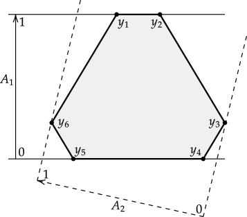
Condition implies that the scalar product takes the value zero for two permutations and the value 1 on at least one permutation. However, as shown in Figure 1, the only outcome that tells apart states from is , which gives probability one for states and zero for . It is worth mentioning that the vectors correspond to four pure states with zero off-diagonal components. Hence, the outcome probabilities of these pure states can be calculated by only looking at the diagonal projection (i.e. the figure).
The figure also shows that, no matter how we choose the direction , the states (or ) cannot be perfectly distinguished. This proves the non-existence of three perfectly distinguishable states in this family of state spaces. Of course, this argument breaks down for the three-level quantum system, when the projection becomes a triangle instead of an hexagon. ∎
The state spaces under consideration (Definition 13) have a remarkable property that is not present in quantum theory. This property is sometimes called “violation of no-simultaneous encoding” [65] and it is very similar to “information causality” [66]. This property allows to perfectly encode one bit of information (e.g. versus ) and simultaneously imperfectly encode another bit ( versus ). Although only one of the two bits can be retrieved, there is a sense in which this system encodes more than one bit of information despite having only two perfectly-distinguishable states. Different choices of will give different success probability when optimally guessing the second bit. This is a statistical feature that distinguishes inequivalent values of within the family of state spaces of Definition 13.
4.4 Continuous deformation of probabilistic structures: the general case
In the following we only consider systems up to tomographic equivalence, where two systems are tomographically equivalent if and and only if they have the same equivalence classes of ensembles (i.e. the same mixed states). For a given set of pure states each equivalence class of probabilistic structures induces a map (where ) by Theorem 1. We will define a deformation of a probabilistic structure for as a map between different images of -maps for (since there is a one-to-one correspondence between equivalence classes of probabilistic structures and images of -maps) satisfying certain conditions which we will formalize with the aid of some further definitions. We only consider equivalence classes of probabilistic structures which separate .
For a given dynamical structure let us call the space of all images (equivalently the space of equivalence classes of probabilistic structures ). For a given let us call the space of all whose linear span is isomorphic to (equivalently the space of equivalence classes of probabilistic structures such that ). We observe that might be the empty set (if there are no representations of of the form of Equation (15) acting on ). For a Gelfand dynamical structure all are countable sets, whilst for non-Gelfand pairs there exist which are uncountable.
The symmetrised distance defined in Equation (18) turns into a metric space. This metric induces a topology on .
We are interested in continuously deforming probabilistic structures, namely how to continuously vary one set of mixed states into another (i.e. one probabilistic structure into another) whilst keeping the linear dimension fixed. First we define a general transformation between sets of embedded pure states .
Definition 14 (Trivial -transformation map).
For two systems and with associated maps and we define the trivial -transformation map , (where it acts as , ).
These trivial -transformation maps allow us to map between any two probabilistic structures in . A deformation of probabilistic structure is a specific map between probabilistic structures such that the linear dimension of the space of mixed states is unchanged.
Definition 15 (Deformation map).
For two systems and with associated maps and where a trivial -transformation map , is a deformation map.
Lemma 3.
A non-trivial deformation map () cannot be extended to a linear transformation on .
Proof.
Since and separate , and are homeomorphic. Let us prove by contradiction and assume that is linear when extended to . Let us call this linear extension of . We observe that has a trivial kernel since no element of is in the kernel, hence no element of is either. Moreover the image of is : any element in is a linear combination of elements in , and hence by linearity of is the image under of the linear combination in the domain . Hence is an invertible linear transformation which takes to and . This contradicts the assumption that and are induced by tomographically inequivalent probabilistic structures. ∎
A non-trivial deformation map cannot be extended to the spaces of mixed states and , which are not isomorphic as convex sets. For such systems one can use the map to deform the probabilistic structure to to change the space of mixed states from to whilst preserving the linear dimension.
We observe that if we consider the general trivial -transformation maps (i.e. the linear dimension of the two state spaces is no longer required to be the same) then some of these maps do linearly extend to when . An example of such a map is the projection from a system with an associated representation which is reducible to a system with an associated representation which is a sub-representation of , i.e. for some representation of .
Definition 16 (Continuous deformation of probabilistic structure).
A probabilistic structure can be continuously deformed to another probabilistic structure if there is a continuous function , in with such that and . Here continuity is defined with respect to the usual topology on . defines a connected path in .
We observe that the connected path defines a family of deformation maps for every .
In other words can be continuously deformed to if there exists a connected path between the two passing through a continuum of different (each spanning a linear space of the same dimension). If there is no such path between the two then cannot be continuously deformed to .
In the following theorem we show the relation between the rigidity of a probabilistic structure and the possibility of continuously deforming a probabilistic structure.
Lemma 4.
Any non-rigid probabilistic structure can be continuously deformed into another (non-rigid) probabilistic structure . Any rigid probabilistic structure cannot be continuously deformed to another probabilistic structure.
This lemma is proven in Appendix E.3. Together with Corollary 1 this lemma implies the following corollary.
Corollary 2.
If is a Gelfand pair, then no probabilistic structure can be continuously deformed. If is a non-Gelfand pair then it has probabilistic structures which can be continuously deformed.
We now provide an explicit construction of a continuous deformation of a probabilistic structure whose associated representation has inequivalent -invariant vectors; for an arbitrary non-Gelfand pair .
Example 1 (Continuous deformation).
Consider a non-Gelfand pair , and an irreducible spherical representation acting on with inequivalent -invariant vectors and (which always exists for a given non-Gelfand pair). Any vector in is -invariant, moreover any two vectors in which are not proportional will generate inequivalent state spaces under . Let us take two inequivalent normalised -invariant vectors and . Let us call and the two embedded sets of pure states generated from these two reference vectors. Consider a rotation such that . For a given state and we have the relation:
| (57) |
Hence there is a map between the two points and , for all points . The deformation map is then:
| (58) | ||||
| (59) |
Since this map is -dependent (i.e. its action depends on each extremal point ) it is not linear and cannot be extended to the mixed states.
Let us define to be the state space generated by the -invariant reference vector for and . Then the deformation map from to is given by:
| (60) | ||||
| (61) |
The family of deformation maps (for ) defines a connected path in (see the proof of Lemma 4 in Appendix E.3). Hence the probabilistic structure associated to can be continuously deformed to the probabilistic structure associated to .
Remark 4.
The possibility of continuously deforming a probabilistic structure without altering its dynamical structure (and without restricting effects) is a very peculiar feature that is not found in any of the known GPTs (such as boxworld and quantum theory over the field of reals, complex or quaternions) to the best of our knowledge. Moreover we posit that this is a typical feature of GPT systems, in that, most dynamical structures are not Gelfand pairs. If a probabilistic structure can be continuously deformed then the probabilities can be fine-tuned to suitably describe the observed statistics, and hence, make the theory more difficult to falsify. Hence, the fact that the probabilistic structure of a theory cannot be smoothly deformed makes the falsifiability of the theory more straightforward. We believe that this is a desirable property of a theory. If we consider a dynamical structure being a Gelfand pair then we can be sure that any of its probabilistic structures will be straightforwardly falsifiable. Finally, it is important to mention that a dynamical structure cannot be continuously deformed due to the group and sub-group structures of and . That is, adding a single element to or will generate lots of new elements via products and inverses. And hence, the probabilistic structure is the only part of a theory that, a priori, could be continuously deformed.
5 Gelfand pairs and two point homogeneity
In Theorem 2 we have singled out dynamical structures corresponding to Gelfand pairs as being of interest, namely for the convenient property that their probabilistic structures can be classified via the associated group representations. This implies that there are countably many of them, and that they cannot be continuously deformed. This rigidity is a highly desirable property for a fundamental theory of physics, because it does not allow for ad hoc parameter adjustment, and is thereby easier to falsify. Apart from this, one may also ask whether there are other informational/physical motivations for considering Gelfand pairs. One such reason may be the following.
Definition 17 (Two-point homogeneous action [67]).
A group acts two-point homogeneously on a metric space if for every pair of points and in with there is an element such that and .
Two-point homogeneity implies transitivity, since for any points and we have and hence there exists an element such that . The following is a very remarkable result.
Lemma 5 (Prop 2.2 [68]).
If acts two-point homogeneously on a metric space and is the stabilizer of a point, then is a Gelfand pair.
The requirement of two-point homogeneity restricts us to dynamical structures corresponding to Gelfand pairs. We observe that this requirement requires an additional metric structure to be imposed on the dynamical structure. A natural metric on GPT state spaces is the following.
Lemma 6.
(Pure-state metric distance.) The distance between any pair of pure states defined by
| (62) |
is bounded , it satisfies the metric axioms:
-
1.
if and only if ,
-
2.
,
-
3.
,
and it is -invariant
-
4.
for all .
Therefore we conclude that two-point homogeneous state spaces are Gelfand pairs. It is remarkable that the purely dynamical property of two-point homogeneity implies that all probabilistic structures are rigid.
However we note that not all Gelfand pairs give rise to a homogeneous space which is two-point homogeneous. Indeed the classification of all the compact and connected two point homogeneous symmetric spaces was given in [67]. These are listed in Table 1.
The full classification of all finite dimensional probabilistic structures for the compact connected two point homogeneous spaces (where all pairs corresponding to such spaces are given in Table 1) directly follows from the classification of all irreducible spherical representations. Equivalently these are the irreducible subspaces of the function space (continuous functions from to ) under the action of , where a specific basis for an irreducible subspace is given by spherical harmonics. This is a generalisation of the well known spherical harmonics for , where the irreducible representation labelled by has a basis spanning a dimensional subspace.
The spherical irreducible representations for these pairs are characterised by a condition on the highest weights given by the Cartan-Helgason Theorem [69, 70](see [71, Theorem 11.4.10.]. Explicit characterisations of these spherical irreducible representations (either in terms of the highest weights or other methods) for the pairs in Table 1 can be found in the literature.
6 Grassmannian systems
In this section we introduce a family of non-classical systems which generalise the dynamical structure of quantum systems, and make use of Theorem 2 to provide a full classification of these systems.
The pure states of finite dimensional quantum systems are given by . This is the set of all one dimensional subspaces of . We now consider systems with pure states given by the set of all -dimensional subspaces . This set is known as a Grassmann manifold :
| (63) |
Hence . Since acts transitively on it can also be expressed as follows (re-parametrising and ):
| (64) |
Here the embedding of into is the direct sum embedding:
| (65) |
Similarly one can define Grassmann manifolds over and , generalising the dynamical structures of quantum theory over and . These are:
| (66) | |||
| (67) |
In the next section we will make use of Theorem 2 to classify all possible probabilistic structures for each dynamical structure which is a complex Grassmann manifold.
6.1 Full classification of all probabilistic structures for complex Grassmann manifolds
Theorem 2 states that for a dynamical structure corresponding to a Gelfand pair, every probabilistic structure is in one-to-one correspondence with a spherical representation of . Hence the first step in classifying probabilistic structures for the Grassmann dynamical structure is to determine whether form a Gelfand pair.
Lemma 7.
-
1.
form a Gelfand pair.
-
2.
The spherical representations have a real structure.
The first part of the lemma is found in [72, Corollary 3] and the second part is proven in Appendix F. This lemma entails (using Theorem 2) that all probabilistic structures where are in one-to-one correspondance with the spherical representations . Irreducible spherical representations are typically defined over , and in general the irreducible representations of a group over are not in one-to-one correspondence with those over . Part 2. of the lemma allows us to classify the real irreducible spherical representations of by studying the irreducible spherical representations over .
The restriction of representations of to has been studied in [72]. We summarise the result below. Representations of are labelled by a partition of an integer in parts (often represented as a Young diagram). One can construct the associated irreducible representation by applying the Schur functor to [73, Proposition 15.15]
Lemma 8.
The representations of which have a trivial representation when restricted to are of the following form: When :
| (68) |
When :
| (69) |
In each case . We have added a redundant 0 entry; with it has length .
6.2 Quartic quantum theory over and
Quartic quantum theory over , introduced in [47], is a theory which contains some of the systems classified above. In this theory systems () have pure states given by the Grassman manifold and a probabilistic structure given by the adjoint representation. For example the state space for the system can be generated by taking reference state:
| (70) |
applying the dynamical group in the adjoint representation:
| (71) |
and taking the convex hull of the manifold embedded in (the real linear space of Hermitian matrices on ).
One problematic feature of quartic quantum theory is that it does not have well defined composition [47, 25], and as such is just a collection of systems rather than a full theory.
We can similarly introduce two theories (without composition): real quartic quantum theory and quaternionic quartic quantum theory where systems are given by and , where and are acted on by the adjoint representation of and respectively. In both cases the states space for the system associated to can be generated by taking the reference state above acting with the adjoint representation of the dynamical group and taking the convex hull.
7 Discussion
7.1 Comparison to previous work
7.1.1 The generalised quantum mechanics of Mielnik
The OPF framework presented in this work is similar to the ‘Group theoretical model’ of [10]. The novel aspects of this work include Theorem 2 which, building on the framework, establishes a correspondence between probabilistic structures and group representations. We find specific conditions on transitive dynamical structures which make this correspondence one-to-one (namely that the dynamical group and stabilizer subgroup form a Gelfand pair). Moreover Mielnik studies examples with the same pure states as quantum theory, but different dynamical groups. We study (and classify) systems which have different pure states and dynamics.
7.1.2 Classification of all alternatives to the measurement postulates of quantum system
Theorem 2 is a generalisation of the classification theorem of [51], where the dynamical structure is no longer constrained to be that of quantum systems. We also find the necessary and sufficient conditions for which dynamical structures have probabilistic structures which are in one-to-one correspondence with group representations.
7.2 Mapping the space of GPT systems
In the GPT formalism a theory is considered to be a set of systems together with some composition rules. Quantum theory for example is the set of systems together with the standard tensor product composition rule and partial trace. We note that alone is not a theory, just a set of systems.
In this work we also consider sets of systems which are not expected to form theories; these are sets of systems which share a common dynamical structure. For example the set of systems with shared dynamical structure form a sub-family of systems, and the set of systems which contain all systems with dynamical structure () form a family of systems.
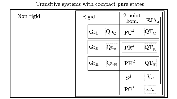
In this work we have introduced new families of systems (see Sections 5 and 6) which generalise previously known systems. In Figure 2 we map out the space of transitive systems with compact pure states including the new families of systems introduced in this work.
The advantage of the methods introduced in this work are two-fold: firstly we can generate examples of non-classical systems and secondly we can systematically classify non-classical systems, thus providing us with a fuller picture of non-classical systems lying beyond quantum theory.
7.3 The search for alternative theories and the issue of composition
The tools presented in this work allow us to systematically search for non-classical systems. However it is not certain that these systems compose in a non-trivial manner (existence of entangled states and measurements). For example it is shown in [53] that the only full theory with systems having the same dynamical structure as quantum theory is quantum theory itself. In [48] it is shown (under certain additional assumptions such as local tomography) that the only systems corresponding to -balls which compose non-trivially are for . However, removing the requirement of local tomography allows for d-balls to compose non-trivially in at least some cases, including those of real and quaternionic bits [35] (where a category in which arbitrary d-balls combine via a monoidal product is also described, though the acceptability of these composites is less clear). Out of the family of systems classified in section 6 it is known that one of them (quartic quantum theory) does not compose under the assumption of local tomography and the requirement that the theory remain quartic [47, 25]. The question remains open as to whether any of the systems with pure states given by Grassmann manifolds compose non-trivially, with or without the assumption of local tomography
8 Conclusion
In this work we have introduced the OPF framework which is used to characterise systems in GPTs. By separating the dynamical and probabilistic components of systems this framework provides new insight into non-classical systems. It allows us to consider families of systems which share a common dynamical structure. We introduce the notion of a rigid dynamical structure and show that for such structures one can classify all probabilistic structures using representations of the dynamical group. A key feature of rigid dynamical structures is that they do not admit continuous deformation of probabilistic structure.
Moreover we introduced multiple new families of non-classical systems, such as the complex Grassmann systems. Many of these families contain known non-classical systems, as well as providing infinitely many examples of non-classical systems which were not known. As well as exploring the space of non-classical systems by finding new examples, we mapped out this space in a more systematic manner by introducing families of systems which share a dynamical structure.
The present work has limited itself to single systems. In general it is not a given that these systems can be made to compose in a non-trivial way (i.e. with entangled states). Future work will involve extending the OPF framework to include composition (along the lines of [52, 53]) and determining whether any of the new families of systems presented in this work can compose in a non-trivial manner. Finding such examples would provide new non-classical theories whose informational properties could be characterised and contrasted to quantum theory. Alternatively a proof that none of the Grassmann systems can compose would lend credence to the proposition that there are few fully compositional general probabilistic theories.
9 Acknowledgements
We thank the referees for their detailed reports which helped substantially improve the present paper, both in terms of fixing errors in proofs and leading to a more rigorous notion of deformation of probabilistic structure. TG acknowledges helpful discussions with Jon Yard. LM acknowledges financial support by the UK’s Engineering and Physical Sciences Research Council [grant number EP/R012393/1]. This research was supported in part by Perimeter Institute for Theoretical Physics. Research at Perimeter Institute is supported by the Government of Canada through the Department of Innovation, Science and Economic Development and by the Province of Ontario through the Ministry of Research, Innovation and Science.
References
- Segal [1947] I. E. Segal, Postulates for general quantum mechanics, Annals of Mathematics 48, 930–948 (1947).
- Mackey [1963] G. W. Mackey, Mathematical Foundations of Quantum Mechanics (A. Benjamin, Inc., New York, 1963).
- Ludwig [1964] G. Ludwig, Versuch einer axiomatischen Grundlegung der Quantenmechanik und allgemeinerer physikalischer Theorien, Zeitschrift für Physik 181, 233–260 (1964).
- Ludwig [1967] G. Ludwig, Attempt of an axiomatic foundation of quantum mechanics and more general theories. II, Comm. Math. Phys. 4, 331–348 (1967).
- Ludwig [1968] G. Ludwig, Attempt of an axiomatic foundation of quantum mechanics and more general theories. III, Communications in Mathematical Physics 9, 1–12 (1968).
- Dähn [1968] G. Dähn, Attempt of an axiomatic foundation of quantum mechanics and more general theories. IV, Communications in Mathematical Physics 9, 192–211 (1968).
- Stolz [1969] P. Stolz, Attempt of an axiomatic foundation of quantum mechanics and more general theories. V, Communications in Mathematical Physics 11, 303–313 (1969).
- Stolz [1971] P. Stolz, Attempt of an axiomatic foundation of quantum mechanics and more general theories VI, Communications in Mathematical Physics 23, 117–126 (1971).
- Mielnik [1969] B. Mielnik, Theory of filters, Communications in Mathematical Physics 15, 1–46 (1969).
- Mielnik [1974] B. Mielnik, Generalized quantum mechanics, Communications in Mathematical Physics 37, 221–256 (1974).
- Giles [1970] R. Giles, Foundations for Quantum Mechanics, Journal of Mathematical Physics 11, 2139 (1970).
- Gudder [1973] S. Gudder, Convex structures and operational quantum mechanics, Communications in mathematical Physics 29, 249–264 (1973).
- Davies and Lewis [1970] E. B. Davies and J. T. Lewis, An operational approach to quantum probability, Communications in Mathematical Physics 17, 239–260 (1970).
- Hardy [2001] L. Hardy, Quantum theory from five reasonable axioms, eprint arXiv:quant-ph/0101012 (2001), quant-ph/0101012 .
- Barrett [2007] J. Barrett, Information processing in generalized probabilistic theories, Phys. Rev. A 75, 032304 (2007).
- Dakic and Brukner [2011] B. Dakic and C. Brukner, Quantum Theory and Beyond: Is Entanglement Special?, in Deep Beauty - Understanding the Quantum World through Mathematical Innovation, edited by H. Halvorson (Cambridge University Press, 2011) pp. 365–392.
- Masanes and Muller [2011] L. Masanes and M. P. Muller, A derivation of quantum theory from physical requirements, New Journal of Physics 13, 063001 (2011).
- Chiribella et al. [2011] G. Chiribella, G. M. D’Ariano, and P. Perinotti, Informational derivation of quantum theory, Physical Review A 84, 012311 (2011).
- Barnum and Wilce [2011] H. Barnum and A. Wilce, Information processing in convex operational theories, Electronic Notes in Theoretical Computer Science 270, 3 – 15 (2011).
- Barnum et al. [2013] H. Barnum, R. Duncan, and A. Wilce, Symmetry, compact closure and dagger compactness for categories of convex operational models, Journal of Philosophical Logic 42, 501–523 (2013).
- Chiribella et al. [2010] G. Chiribella, G. M. D’Ariano, and P. Perinotti, Probabilistic theories with purification, Physical Review A 81, 062348 (2010).
- Garner et al. [2013] A. J. P. Garner, O. C. O. Dahlsten, Y. Nakata, M. Murao, and V. Vedral, A framework for phase and interference in generalized probabilistic theories, New Journal of Physics 15, 093044 (2013).
- Barnum et al. [2014] H. Barnum, M. P. Muller, and C. Ududec, Higher-order interference and single-system postulates characterizing quantum theory, New Journal of Physics 16, 123029 (2014).
- Barnum et al. [2017] H. Barnum, C. Lee, C. Scandolo, and J. Selby, Ruling out Higher-Order Interference from Purity Principles, Entropy 19, 253 (2017), arXiv:1704.05106 [quant-ph] .
- Lee and Selby [2017] C. M. Lee and J. H. Selby, Higher-order interference in extensions of quantum theory, Foundations of Physics 47, 89–112 (2017).
- Muller and Ududec [2012] M. P. Muller and C. Ududec, Structure of reversible computation determines the self-duality of quantum theory, Phys. Rev. Lett. 108, 130401 (2012).
- Lee and Barrett [2015] C. M. Lee and J. Barrett, Computation in generalised probabilisitic theories, New Journal of Physics 17, 083001 (2015), arXiv:1412.8671 [quant-ph] .
- Brunner et al. [2014] N. Brunner, M. Kaplan, A. Leverrier, and P. Skrzypczyk, Dimension of physical systems, information processing, and thermodynamics, New Journal of Physics 16, 123050 (2014).
- Chiribella and Scandolo [2015] G. Chiribella and C. M. Scandolo, Operational axioms for diagonalizing states, EPTCS 2, 96–115 (2015).
- Chiribella and Scandolo [2015] G. Chiribella and C. M. Scandolo, Entanglement and thermodynamics in general probabilistic theories, New Journal of Physics 17, 103027 (2015).
- Barnum et al. [2010] H. Barnum, J. Barrett, L. Orloff Clark, M. Leifer, R. Spekkens, N. Stepanik, A. Wilce, and R. Wilke, Entropy and information causality in general probabilistic theories, New Journal of Physics 12, 033024 (2010), arXiv:0909.5075 [quant-ph] .
- Kimura et al. [2010] G. Kimura, K. Nuida, and H. Imai, Distinguishability measures and entropies for general probabilistic theories, Reports on Mathematical Physics 66, 175 – 206 (2010).
- Janotta et al. [2011] P. Janotta, C. Gogolin, J. Barrett, and N. Brunner, Limits on nonlocal correlations from the structure of the local state space, New Journal of Physics 13, 063024 (2011).
- Janotta and Lal [2013] P. Janotta and R. Lal, Generalized probabilistic theories without the no-restriction hypothesis, Physical Review A 87, 052131 (2013).
- Barnum et al. [2020] H. Barnum, M. A. Graydon, and A. Wilce, Composites and Categories of Euclidean Jordan Algebras, Quantum 4, 359 (2020).
- Bae et al. [2016] J. Bae, D.-G. Kim, and L.-C. Kwek, Structure of optimal state discrimination in generalized probabilistic theories, Entropy 18, 39 (2016).
- Selby and Sikora [2018] J. H. Selby and J. Sikora, How to make unforgeable money in generalised probabilistic theories, Quantum 2, 103 (2018).
- Heinosaari et al. [2019] T. Heinosaari, L. Leppäjärvi, and M. Plávala, No-free-information principle in general probabilistic theories, Quantum 3, 157 (2019).
- Davies [1972] E. Davies, Example Related to the Foundations of Quantum Theory, Journal of Mathematical Physics 13, 39–41 (1972).
- Short and Barrett [2010] A. J. Short and J. Barrett, Strong nonlocality: a trade-off between states and measurements, New Journal of Physics 12, 033034 (2010).
- Gross et al. [2010] D. Gross, M. Muller, R. Colbeck, and O. C. O. Dahlsten, All reversible dynamics in maximally nonlocal theories are trivial, Phys. Rev. Lett. 104, 080402 (2010).
- Al-Safi and Short [2014] S. W. Al-Safi and A. J. Short, Reversible dynamics in strongly non-local boxworld systems, Journal of Physics A: Mathematical and Theoretical 47, 325303 (2014).
- Hardy and Wootters [2012] L. Hardy and W. K. Wootters, Limited Holism and Real-Vector-Space Quantum Theory, Foundations of Physics 42, 454–473 (2012), arXiv:1005.4870 [quant-ph] .
- Aleksandrova et al. [2013] A. Aleksandrova, V. Borish, and W. K. Wootters, Real-vector-space quantum theory with a universal quantum bit, Physical Review A 87, 052106 (2013).
- Wootters [2013] W. K. Wootters, Optimal Information Transfer and Real-Vector-Space Quantum Theory, arXiv eprints:quant-ph/1301.2018 (2013).
- Finkelstein [1959] D. N. Finkelstein, Notes on Quaternion Quantum Mechanics, CERN publications: European Organization for Nuclear Research (CERN, 1959).
- Życzkowski [2008] K. Życzkowski, Quartic quantum theory: an extension of the standard quantum mechanics, Journal of Physics A: Mathematical and Theoretical 41, 355302 (2008).
- Masanes et al. [2014] L. Masanes, M. P. Mueller, D. Perez-Garcia, and R. Augusiak, Entanglement and the three-dimensionality of the Bloch ball, Journal of Mathematical Physics 55, 122203 (2014).
- Krumm and Müller [2019] M. Krumm and M. P. Müller, Quantum computation is the unique reversible circuit model for which bits are balls, npj Quantum Information 5, 7 (2019), arXiv:1804.05736 [quant-ph] .
- Dakić et al. [2014] B. Dakić, T. Paterek, and C. Brukner, Density cubes and higher-order interference theories, New Journal of Physics 16, 023028 (2014).
- Galley and Masanes [2017] T. D. Galley and L. Masanes, Classification of all alternatives to the Born rule in terms of informational properties, Quantum 1, 15 (2017).
- Galley and Masanes [2018] T. D. Galley and L. Masanes, Any modification of the Born rule leads to a violation of the purification and local tomography principles, Quantum 2, 104 (2018).
- Masanes et al. [2019] L. Masanes, T. Galley, and M. P. Muller, The measurement postulates of quantum mechanics are operationally redundant, Nature Communications 10, 1361 (2019).
- Wilce [2009] A. Wilce, Four and a half axioms for finite dimensional quantum mechanics (2009), arXiv:0912.5530 [quant-ph] .
- Rio et al. [2011] L. d. Rio, J. Åberg, R. Renner, O. Dahlsten, and V. Vedral, The thermodynamic meaning of negative entropy, Nature 474, 61–63 (2011).
- Horodecki and Oppenheim [2013] M. Horodecki and J. Oppenheim, Fundamental limitations for quantum and nanoscale thermodynamics, Nature Communications 4, 2059 (2013).
- Brandão et al. [2013] F. G. S. L. Brandão, M. Horodecki, J. Oppenheim, J. M. Renes, and R. W. Spekkens, Resource theory of quantum states out of thermal equilibrium, Physical Review Letters 111, 250404 (2013).
- Skrzypczyk et al. [2014] P. Skrzypczyk, A. J. Short, and S. Popescu, Work extraction and thermodynamics for individual quantum systems, Nature Communications 5, 4185 (2014).
- Brandão et al. [2015] F. Brandão, M. Horodecki, N. Ng, J. Oppenheim, and S. Wehner, The second laws of quantum thermodynamics, Proceedings of the National Academy of Sciences 112, 3275–3279 (2015).
- Hofmann and Morris [2013] K. H. Hofmann and S. A. Morris, The structure of compact groups : a primer for students, a handbook for the expert, third edition, revised and augmented ed. (Berlin, Boston: De Gruyter, 2013).
- Gallier [2018] J. H. Gallier, Advanced geometric methods in computer science, https://www.cis.upenn.edu/~cis610/cis610-18-sl18.pdf (2018), chapter 20: Manifolds arising from group actions.
- Mazurek et al. [2021] M. D. Mazurek, M. F. Pusey, K. J. Resch, and R. W. Spekkens, Experimentally bounding deviations from quantum theory in the landscape of generalized probabilistic theories, PRX Quantum 2, 020302 (2021).
- Sanyal et al. [2011] R. Sanyal, F. Sottile, and B. Sturmfels, Orbitopes, Mathematika 57, 275–314 (2011).
- Vesely [2010] L. Vesely, Extreme points of compact convex sets, http://www.mat.unimi.it/users/libor/AnConvessa/ext.pdf (2010), NoStop
- Masanes et al. [2013] L. Masanes, M. P. Muller, R. Augusiak, and D. Perez-Garcia, Existence of an information unit as a postulate of quantum theory, Proceedings of the National Academy of Sciences 110, 16373–16377 (2013).
- Pawłowski et al. [2009] M. Pawłowski, T. Paterek, D. Kaszlikowski, V. Scarani, A. Winter, and M. Żukowski, Information causality as a physical principle, Nature 461, 1101–1104 (2009).
- Wang [1952] H.-C. Wang, Two-point homogeneous spaces, Annals of Mathematics 55, 177–191 (1952).
- Gross [1991] B. H. Gross, Some applications of gelfand pairs to number theory, Bull. Amer. Math. Soc. (N.S.) 24, 277–301 (1991).
- Cartan [1929] E. Cartan, Sur la détermination d’un système orthogonal complet dans un espace de Riemann symétrique clos, Rendiconti del Circolo Matematico di Palermo (1884-1940) 53, 217–252 (1929).
- Helgason [1984] S. Helgason, Groups and geometric analysis: integral geometry, invariant differential operators, and spherical functions, Pure and applied mathematics No. 113 (Academic Press, Orlando, 1984).
- Wolf [2007] J. Wolf, Harmonic Analysis on Commutative Spaces, Mathematical Surveys and Monographs, Vol. 142 (American Mathematical Society, Providence, Rhode Island, 2007).
- Halima [2007] M. B. Halima, Branching rules for unitary groups and spectra of invariant differential operators on complex Grassmannians, Journal of Algebra 318, 520–552 (2007).
- Fulton and Harris [1991] W. Fulton and J. Harris, Representation theory : a first course, Graduate texts in mathematics (Springer-Verlag, New York, Berlin, Paris, 1991).
- Sepanski [2007] M. R. Sepanski, Compact Lie Groups, 1st ed. (Springer-Verlag New York, 2007).
- Holevo [2011] A. S. Holevo, Probabilistic and statistical aspects of quantum theory, 2nd ed., Quaderni Monographs No. 1 (Edizioni della normale, Pisa, 2011).
Appendix A Notation
| System with pure states | |
| Symmetric group on set | |
| Group of diffeomorphisms on manifold | |
| Image of map for en element | |
| The set | |
| Convex hull of | |
| Ensemble of pure states | |
| Mixed state representation of an ensemble | |
| set of OPFs (outcome probability functions) for system with pure states | |
| Extension of an OPF to ensembles/mixed states | |
| Representation of a group on linear space over | |
| Multiplicity of the sub-representation in the representation | |
| Linear space of -equivariant maps from to | |
| Complexification of a real representation | |
| Restriction to reals of a complex representation | |
| Continuous functions for a topological space and a field | |
| Vector space of functions for finite | |
| G-module (carrier space of a representation of ) | |
| Identity operator on | |
| Complex conjugate vector space | |
| Complex conjugate of a vector v |
Appendix B Background group theory and group representation theory
We briefly outline a few concepts from group representation theory which will be needed for the proofs.
B.1 Representation theory basics
Definition 18 (Group representation).
A representation of a group is a homomorphism , where is a finite dimensional vector space. When is a Lie group this is a continuous map. is called the carrier space of the representation, or a -module.
Let us denote by the space of linear maps .
Definition 19 (Intertwining operators).
Let and be representations of . An element is called an intertwining operator if . We denote the linear space of all such maps .
is a subspace of .
Theorem 6 (Schur’s Lemma).
Let and be irreducible representations of over . Then when and otherwise.
This implies that for irreducible . Schur’s Lemma also has important consequences for reducible representations. For instance consider the case where where is irreducible and is reducible. Then Schur’s Lemma entails that must contain the irreducible representation exactly once, and that .
B.2 Left regular and representations
Definition 20 (Left regular representation (finite group)).
The left regular representation of a finite group is given by:
| (72) | |||
| (73) |
where is a complex linear space spanned with orthonormal basis .
Here the action of on is just permutation of the basis vectors.
Definition 21 (Left regular representation (compact group)).
The left regular representation of a compact topological group is given by:
| (74) |
where .
is a continuous homomorphism: .
B.3 Restricted and induced representations
B.3.1 Restricted representation
Definition 22 (Restricted representation).
The restriction of a representation of a group to a subgroup is a representation of on with operators for all . It is denoted .
In general the restriction of an irreducible representation will give a reducible representation .
Example 2.
Consider the fundamental representation of on and restrict to the subgroup with matrices:
| (75) |
This is a reducible representation of containing the trivial and fundamental representation.
B.3.2 Induced representation
Definition 23 (Induced representation: and finite).
A representation of a subgroup of induces a representation of given by the right regular representation of on:
| (76) |
The carrier space is the space of functions which are -equivariant. We can write it as
Definition 24 (Induced representation: locally compact and closed).
A representation of a subgroup of induces a representation of :
| (77) |
The action of on is given by where .
B.4 Frobenius reciprocity
Theorem 7 (Frobenius reciprocity).
[74, Theorem 7.47] Take a finite group and a subgroup or G a Lie group and a closed subgroup of . Given a representation of and a representation of , then as vector spaces
| (78) |
We define (with finite) to be the space of functions which forms a vector space under pointwise addition and scalar multiplication. It carries a representation of , inherited from the action of on . For a topological space, is the vector space of continuous functions , also carrying a representation of .
Corollary 3.
For finite the irreducible representation occurs in with multiplicity equal to the multiplicity of the trivial representation in . For compact the irreducible representation occurs in with multiplicity equal to the multiplicity of the trivial representation in .
Proof.
First observe for finite and for compact .
Let us consider the case where is the trivial representation: . Then contains a trivial representation with multiplicity . Using Schur’s lemma the only -equivariant map from to are identities on the trivial representations. In other words .
Appendix C Representations over
A representation is a homomorphism for some vector space . Typically is assumed to be a vector space over , and many tools in representation theory apply to this case. Schur’s lemma for instance holds for representations over the complex field, but not always for those over . For a Gelfand pair the property of having a trivial irreducible representation when restricted to which is of multiplicity or holds for representations over , and not necessarily .
In this section we explore some of the subtleties involved in dealing with representations over and prove some lemmas which will be needed for Theorem 2. First we present an example to introduce some of the relevant concepts.
Example 3 (Fundamental representation of ).
Consider the representation of over :
| (80) |
This representation is irreducible over . However consider this representation acting on (obtained from by allowing complex linear combinations of the basis elements). Then there exist the following matrices and :
| (81) |
such that , with
| (82) |
So the irreducible representation over is reducible over . Consider once again the irreducible representation over . Then this commutes with all matrices proportional to the identity, but also matrices proportional to , where is:
| (83) |
Moreover one can show that only matrices which are linear combinations of and commute with the whole group.
C.1 Definitions
Definition 25 (Real, complex and quaternionic structure).
Consider an irreducible representation with a complex vector space. Then has a real structure if there exists an equivariant anti-linear map such that , has a quaternionic structure if there exists an equivariant anti-linear map such that . Otherwise has a complex structure.
Lemma 9 (Descent map).
Given a representation of a group over a complex space equipped with a real structure the projection with kernel the eigenspace of is a descent map. carries a real representation of .
Proof.
Consider . Observe that this set is closed under real linear combinations, and not complex linear combinations. As such it has the structure of a real vector space. Moreover .
Since , carries an action of . Moreover for we have for . Therefore carries a real representation of .
∎
Typically is the conjugation map: . We see that it is equivariant when , i.e. the representation and are isomorphic.
Definition 26 (Complexification).
A real vector space has complexification where is a complex vector space. A basis for this complex vector space is . .
We sometimes write .
Definition 27 (Restriction of scalars).
A complex vector space is isomorphic (as a real vector space) to the real vector space . . If is a basis for , then is a basis for .
Consider a complex vector space and a real vector space.
| (84) | |||
| (85) |
where is the complex conjugate vector space of . has the same elements and addition rule as , but scalar multiplication is given by .
Theorem 8.
[73, Theorem 3.37, p.41] For an irreducible representation the action of extends naturally to . It has one of the following decompositions:
-
1.
for a complex irreducible representation if and only if has a real structure.
-
2.
for a complex irreducible representation if and only if has a complex structure.
-
3.
for a complex irreducible representation if and only if has a quaternionic structure.
Every real irreducible representation can be obtained from irreducible complex representations of one of the above three forms, by taking the descent map .
Corollary 4.
Consider the set of all irreducible complex representations of a group , these are the representations of real type, the representation complex type and the representations of quaternionic type. The set of all real irreducible representations has a unique representative element in , where is the set of complex representations where conjugate representations are equivalent.
C.2 Lemmas
In the following section is assumed finite or compact.
Lemma 10.
For a Gelfand pair all irreducible representations with an -invariant subspace have either a real or complex structure.
Proof.
For finite every representation with an -invariant subspace occurs exactly once in the decomposition of by Corollary 3. has a real structure (compatible with the group action) and decomposes as .
By Theorem 8 the complexification map sends every real irreducible representation in to either:
-
1.
An irreducible representation in if is real.
-
2.
A reducible representation in if is complex.
-
3.
A reducible representation in if is quaternionic.
However since only contains single copies of irreps it cannot contain and hence no irrep can be of quaternionic form.
For compact every representation with an -invariant subspace occurs exactly once in the decomposition of by Corollary 3. is the complexification of and the same proof as for the finite case follows through. ∎
Lemma 11.
For a Gelfand pair and an irreducible representation over , then the following holds:
-
1.
If is irreducible over then the (real) dimension of the -invariant subspace in is the same as the (complex) dimension of the -invariant subspace in : . It is either or .
-
2.
If is reducible over then the (real) dimension of the -invariant subspace in is twice that of the (complex) dimension of the -invariant subspace in : . It is either or .
Proof.
-
1.
. The -invariant complex subspace of is 0 or 1 dimensional. Consider the 1 dimensional case, then is spanned by a vector . Now since for the map , we have that under the descent map the subspace is mapped to the (real) one dimensional subspace of , spanned by with . Any vector such that which is not in will be mapped to a vector in which is not -invariant (since is equivariant). As such the subspace of all -invariant vectors in is just and is one dimensional. The case where is of dimension is immediate.
-
2.
By Lemma 10 if is irreducible over but reducible over then it has a complex structure and is of the form where and are irreducible. Since is a Gelfand pair either both and contain a one dimensional -invariant complex subspace or neither do. Let us consider the case where they both do.
(86) We use a matrix representation where the entries of are the complex conjugates of those of . Let be a basis for , then
(87) form a basis for . By also considering the elements:
(88) we obtain a real basis for , i.e. any is a real linear combination of the above vectors.
Let
(89) be an invariant vector, then so is:
(90) All -invariant vectors are of the form:
(91) since the invariant subspaces in and are one dimensional.
Now we consider the change of basis given by matrices and :
(92) and apply to obtain
(93) has real valued entries. The action of on the basis is:
(94) Considering the real basis elements we also obtain:
(95) Under the real structure the basis vectors and are eigenvectors of , and form a basis for . The other basis vectors are eigenvectors and form a basis for . Since we have that and so the subspace is closed under .
The image of the -invariant vectors under is:
(96) These are invariant under for . Any such invariant vector is a real linear combination of and . As such the -invariant subspace in is two dimensional with basis vectors written out explicitly as:
(97) (98)
∎
Corollary 5.
For a Gelfand pair and an irreducible representation over , then all -invariant vectors are related by an invertible transformation which commutes with .
Proof.
In the case where is complex irreducible this is immediate from Schur’s lemma. In the case where is complex reducible, then its complexification is reducible:
| (99) |
By Schur’s lemma all matrices which commute with the whole group are of the form:
| (100) |
Using the transformation of the previous proof one obtains:
| (101) |
which all commute with . This is real valued for , and all real linear combinations of these matrices. and where
| (102) |
Consider the two basis invariant vectors and of Equation (97). These are related by . Therefore all linear combinations of these are related by real linear combinations of and . ∎
Corollary 6.
For an irreducible representation over , then the following holds:
-
1.
If is irreducible then . The only equivariant homomorphisms are scalar multiples of the identity.
-
2.
If is reducible into irreducible representations with complex structure then .
Lemma 12.
For a Gelfand pair of finite groups , the representation of acting on contains exactly once every irreducible representation of which has a trivial sub-representation when restricted to and does not contain any other representations.
Proof.
By Corollary 3 contains every irreducible representation with an invariant subspace with multiplicity 1, if an irreducible is of complex type then its complex conjugate is necessarily also in , since if has a -invariant vector so does .
We have which contains only irreducible representations with complex or real structures by Lemma 10. Therefore we have:
| (103) |
where are the irreducible representations of real type, and are irreducible representations of complex type. There are no degeneracies.
decomposes into real irreducible representations .
| (104) | ||||
| (105) |
Hence every irreducible representation is sent to in . By Theorem 8 these are of the form for irreducible of real type, for of complex type and for of quaternionic type, where we know by Lemma 10 that this latter case does not occur.
Combining the above:
| (106) |
where every real irreducible subspace corresponds to either a subspace or . Since these occur with multiplicity 1, every occurs with multiplicity one in . This implies that every occurs with multplicity 1 in . ∎
Lemma 13.
For a Gelfand pair , where compact and a closed subgroup, the representation of acting on contains exactly once every irreducible representation of which has a trivial sub-representation when restricted to and does not contain any other representations.
Proof.
Direct from proof of Lemma 12 replacing with and with ∎
Appendix D Convex linear state space
In this appendix we derive the convex linear state space associated to a system .
Definition 28 (Preparation space).
The preparation space of consists of the space of all ensembles for finite, which is affinely equivalent to the simplex over the set (i.e. with the simplex with extremal points, corresponding to the Dirac measures on ). When is a topological space, the preparation space consists of all positive normalised measures on , which is the generalised simplex
In some treatments [75] a mixture space is considered, where the mixing operation applies also to ensembles. For example one can take ensembles to prepare an ensemble . In our case we can consider ensembles of ensembles by setting which is an ensemble of pure states and hence in the preparation space. We note that in a mixture space and are two distinct elements, even if there can be no affine functional which separates them, by definition. In the “maximally separated” classical state space, these two ensembles are always equivalent. Therefore there is no loss of generality when considering a preparation space, as opposed to a mixture space.
D.1 Proof of Theorem 1
Proof.
We consider a system where is finite dimensional as a linear space. We consider only a preparation space of finite ensembles for this proof (one can extend to continuous ensembles, but for finite dimensional systems this is not necessary). One can extend the OPFs to the preparation space:
| (107) |
Two ensembles and where for all are equivalent ensembles. We can define the linear form : .
| (108) |
Hence to the ensemble we associate the mixed state , which is naturally an element of . Any two indistinguishable ensembles are mapped to the same mixed state. Now we can map the OPFs to linear functionals in :
| (109) |
By assumption is a continuous group action when is a continuous group. Moreover it extends to as follows
| (110) |
This uniquely extends to and hence is a group representation.
∎
D.2 Proof of Lemma 1
Proof.
Let be an embedding of into with .
can be generated by applying to a reference vector for all . Since is compact the matrices can be made orthogonal. Hence every for some is such that . All are such that with the unit effect, therefore lies in the affine span of which is a dimensional hyperplane. This is the hyperplane composed of all such that . Every can be written as:
| (111) |
in a basis where the first element corresponds to the subspace spanned by the unit effect. Observe that acts trivially on the subspace spanned by the unit effect, and hence decomposes as where is the trivial representation. Observe that the maximally mixed state for an arbitrary is invariant under . Hence it lies fully in the subspace spanned by the unit effect. Therefore can be written as:
| (112) |
where is the zero vector.
Restricting our attention to the affine span of , i.e. ignoring the unit effect subspace we observe that the matrices are orthogonal, hence lies on a sphere centred on .
Since lies on a hypersphere, this implies that no point in lies inside , proving the lemma.
∎
D.3 Proof of Lemma 2
Proof.
In the representation in terms of fiducial OPFs the vectors are bounded. Moreover they are closed, since any limit of physically realisable extremal preparations is indistinguishable from an extremal physical preparation. Hence is a closed and bounded subset of (isomorphic to by the assumption of “Possibility of state estimation using a finite outcome set”), and by the Heine-Borel theorem it is compact in the induced (subspace) topology.
Since is bounded this implies that the absolute value of the matrix entries of are also bounded. Moreover we assume that from a physical point of view the space of transformations must be topologically closed (in the vector space topology of the space of linear transformations ), since any mathematical transformation which can be arbitrarily well approximated by physical transformations is indistinguishable from a physical transformation. This implies that the set is bounded and closed, and hence compact by the Heine-Borel theorem. ∎
D.4 Proof of Theorem 2
Proof.
-
i.
Take with a Gelfand pair and finite. To every we associated a linear functional . Let us call the representation of acting on . In general may be reducible:
(113) We can also decompose states:
(114) We have the following equality:
(115) Since is stabilized by (where is stabilizer of : for all ) we have
(116) This implies
(117) This implies that each has at least one trivial sub-representation.
-
ii.
Let us consider a representation of acting on a real vector space :
(118) such that each has at least one -invariant subspace. Take a reference vector which has support only in the -invariant subspaces, and has support in each subspace . By applying to we obtain , where we observe that has as extremal points, since can be expressed in orthogonal matrices and hence (a hyper-sphere in the affine span of the normalised states, centred on the maximally mixed state) as proven in Lemma 1. By taking the convex set of all linear functionals which give values in we obtain a probabilistic structure.
-
iii.
Since is a Gelfand pair, all real irreducible representations are such that any pair of -invariant vectors are related by an invertible linear transformation . For a representation:
(119) take two -invariant vectors and which have support in every irreducible subspace. These are related by a transformation : which commutes with the group action. We call their orbits under and . Since commutes with the group action . Let us consider the unrestricted effect spaces for both: and . . The set of all effects on is just , hence .
-
iv.
Let us take the case where is not a Gelfand pair. There exist (complex) irreducible representations such that contains more than one trivial sub-representation.
One can obtain a real irreducible representation from by one of the three following methods:
-
(a)
Restriction to of if is of real type.
-
(b)
Restriction to of if is of complex type.
-
(c)
Restriction to of if if of quaternionic type
In each case the real irreducible representation obtained is such that it has invariant -vectors which are not related by a transformation which commutes with the group representation. Let us fix a basis and consider the matrices acting on . Let us pick two -invariant vectors and such that there is no transformation which commutes with the group action such that .
We now show that and can be used (along with ) to define two tomographically inequivalent probabilistic structures, associated with the same carrier space .
Let us call an element in stabilised by and define and . Furthermore let us define for every (and similarly for ). Observe that for any such that we have (and similarly for ). This defines the maps and . We call and the orbits of and under .
We call the set of all linear functionals giving values in on and the set of all linear functionals giving values in on . Necessarily . and define two OPF sets and respectively.
We have constructed two systems and with associated maps and respectively, associated to the same representation . We now show that these two systems are tomographically inequivalent, i.e. the mixed states and are not isomorphic. In other words there is no linear invertible transformation mapping to .
Consider an invertible linear transformation such that (if such a transformation exists, then it is well defined on the convex hulls and maps to ). This implies that for some fixed and for all pure states . Let us redefine such that the equality for all holds.
Since the state spaces are transitive we have for reference state , and . Using we obtain:
(120) Moreover from we obtain
(121) Hence there is a transformation which commutes with the group action such that . This is in contradiction with the assumption that the two reference states were not related by such a transformation.
-
(a)
∎
Appendix E Deformation of probabilistic structure
E.1 Proof of Theorem 3
Proof.
Let be the representation of associated to , let be the representation of pure states, and let be the representation of OPFs, for . We can decompose the group action into (real) irreducible representations as , , , where Recall that there must be one (and only one) trivial irrep, which we label by . Also, we can decompose the representation of pure states and , and the representation of OPFs and . Within this proof we follow the convention that
| (122) |
for all , where is a group-invariant scalar product. This scalar product provides an isomorphism . Using this decomposition we can write any as
| (123) |
where we define
| (124) |
Schur’s Lemma tells us that any non-trivial irreducible representation satisfies . Therefore, only the trivial rep survives the following average
| (125) |
Next we use another consequence of Schur’s Lemma, namely that for any pair of (real) inequivalent irreducible representations and we have
| (126) |
for any vectors in and any vectors in . Also, if the real irreducible representation has complexification with real structure then
| (127) | ||||
| (128) | ||||
| (129) |
where is the dimension of and are any vectors in .
The case where the real irreducible representation acts on the complexified space as the direct sum of two complex irreducible representations , with complex structure and one being the dual of the other. For what follows we are interested in elements of of the form where is the complex conjugate of , and analogously for . Proceeding as above and using Schur’s Lemma we obtain
| (130) | ||||
| (131) | ||||
| (132) |
where is the dimension of (and ). The structure of the vector implies
| (133) |
and analogously for . Which in turn implies
| (134) |
In summary, the above average is independent of whether the complexification of representation is reducible or not.
The remaining case, where has quaternionic structure, need not be considered, because Lemma 7 proves that it never appears in Gelfand systems. Next we use the identities (126) and (134), the normalisation convention (122) and definition (124) to calculate the following average
| (135) | ||||
where .
Now, suppose that and are unrestricted and tomographically-inequivalent probabilistic structures of . Then, without loss of generality, we assume that irrep is inequivalent to irrep for all . Also, let us choose so that its corresponding vector only has support on the subspaces , that is
| (136) |
This choice is possible because the probabilistic structure is unrestricted. Also, due to the fact that we are obtaining a lower bound for the distance , we do not need to maximise over OPFs , it is enough to pick any one. Next, let us lower-bound the distance between the chosen OPF and any given OPF as
| (137) |
for any . This bound is independent of whether the probabilistic structures and are equivalent or not. Now, using Schur’s lemma as in (125) and (135) we obtain
| (138) |
for any , therefore
| (139) |
Again, using the fact that we can pick any , we further restrict (136) to
| (140) |
for any fixed state . The above is an OPF because the normalisation condition (122) implies that it takes values within . This chosen OPF (140) has , which when substituted in (139) gives
| (141) |
which is the statement of Theorem 3. ∎
E.2 Proof of Theorem 4
E.2.1 Proof of Theorem 4
Proof.
Let of dimension be an unrestricted probabilistic structure of with associated representation such that all -invariant vectors are related by invertible transformations which commute with .
Consider two such vectors and where , with . We can generate state spaces with extremal points by applying to the reference states:
| (142) | |||
| (143) |
Both the state spaces and are related by an invertible transformation and hence are equivalent as convex sets. In other words they correspond to tomographically equivalent probabilistic structures. Since we are only considering unrestricted probabilistic structures they both generate the same state space corresponding to (the linear transformation is just a change of co-ordinates, including rescalings). For probabilistic structures whose -invariant vectors are all related to each other by invertible transformations which commute with there is a unique unrestricted probabilistic structure associated to .
Therefore the only other probabilistic structures such that (if they exist) are associated to different representations . The largest dimensional irreducible representation they can differ by is of dimension (corresponding to the case where either or consists of a dimensional irreducible representation and the trivial and the other representation consists of the trivial representation and an inequivalent irreducible representation or some reducible representation of total dimension ). Therefore by Theorem 3 the distance between the two probabilistic structures is lower bounded by . Any other possibility (i.e. both consist of a trivial representation and different reducible ones would give a lower bound which is higher). ∎
E.2.2 Proof of Theorem 4
Let of dimension be an unrestricted probabilistic structure of with associated representation such that there are pairs of -invariant vectors not related by invertible transformations which commute with . These -invariant vectors belong to an -invariant subspace .
Take and where with . Take for small . We then expand:
| (144) |
We consider a first order approximation and ignore terms of order and higher.
The image of a point is and :
| (145) |
Let us take an OPF with associated effect and an OPF with associated effect :
| (146) | ||||
| (147) |
For a fixed we want to find an which minimizes the distance.
| (148) |
We observe that that the transformations and leave the normalisation degree of freedom (component in the normalisation subspace ) unchanged, therefore if we take then we can choose to obtain .
For any effect with support outside the normalisation subspace the expression (148) is not linear in (due to the last term) and as such there is no choice of which will make cancel out with for all , which is needed to make the distance go to 0. Hence for not proportional to we have the bound:
We observe that every is close to , therefore any which is not tight on (i.e. which gives values in ) will be valid on . Let us minimize the distance for the choice of not tight. We observe that by choosing we obtain:
| (149) |
which implies that
| (150) |
Finally if is tight (i.e. has some values in or ), one can take and add noise (i.e. take ) in order to obtain an effect which is valid on :
E.3 Proof of Lemma 4
Proof.
Two convex sets and with pure states linearly embedded in isomorphic spaces (i.e. for which there exist injective maps and and ) can be continuously deformed one into the other if there exists a path connected map in the space (of maps with codomain ) parametrised by . is an embedding of in for every . We observe that is defined just on the extremal points of (and is invertible), but cannot be extended to by Lemma 3. A connected path on (the space of maps with codomain ) is a continuous map from (with the usual topology) to (with the topology inherited from the metric ).
We now show that for any non-rigid probabilistic structure one can find probabilistic structures which can be continuously deformed into one another, whilst rigid probabilistic structures cannot be continuously deformed.
In the following we make use of the isomorphism and label points in by their stabilizer subgroup. The point with stabilizer subgroup is written as , and any point is written as .
A probabilistic structure is non-rigid if the associated representation contains an irreducible spherical representation with inequivalent -invariant vectors and . Two -invariant vectors and are inequivalent if they are not related by an invertible transformation which commutes with .
We show that a non-rigid probabilistic structure associated to an irreducible representation can be continuously deformed. The case of a non-rigid probabilistic structure associate to a reducible representation follows since one can deform the full reducible probabilistic structure by deforming the subspace of acted on by the irreducible representation with inequivalent -invariant vectors.
The embedded pure state associated to can be generated as , where is an -invariant vector. Let be an inequivalent -invariant vector. Any vector in is -invariant, moreover any two vectors in which are not proportional will generate inequivalent state spaces under . Let us call the embedded sets of pure states generated from the reference state . We now show that can be continuously deformed to .
Consider a rotation such that .
Let us write with for some non-unique generator .
We now show the existence of a connected path in from to , the two sets pure states generated by two non-equivalent -invariant vectors and .
Let us define the state space generated by the -invariant reference vector .
We now define , where . We observe that and . We now show that is a continuous function (where has the topology induced by the metric of Equation (18))
is continuous at a point if for every it is the case that if (for ) then we can find a such that implies .
For large (but ) this holds since one can just take to be small, in which case by the proof of Theorem 4 which is less than or equal to .
If (and greater than ) then setting gives which implies using the proof of Theorem 4 .
This holds for all hence is a continuous function from to with extremal points and . Hence there is a connected path from and in the space of deformation maps, meaning that can be continuously deformed to .
In the case where is a rigid probabilistic structure it is at a finite bounded distance from every other probabilistic structure in by definition. Consider the associated set of embedded pure states and take an arbitrary path to an arbitrary . is not continuous at , since for lower than the finite bounded distance from to any other probabilistic structure, there is no such that implies .
∎
Appendix F Proof of Lemma 7 part 2
Proof.
We make use of Proposition 26.24 of [73] which we translate slightly:
Lemma 14.
Any irreducible representation of with Dynkin indices is complex if for any , real if for all and is odd, or , or and is even, and quaternionic if for all and is odd.
When :
| (155) |
where this has entries.
For all , hence for odd and these are all real. For we observe that (the central entry) is and hence even. This implies the representation is real.
When :
| (156) |
where this has entries.
For all , hence for odd and these are all real. For we observe that (the central entry) is and hence even. This implies the representation is real.
∎
