A Simple General Approach to Balance Task Difficulty in Multi-Task Learning
Abstract
In multi-task learning, difficulty levels of different tasks are varying. There are many works to handle this situation and we classify them into five categories, including the direct sum approach, the weighted sum approach, the maximum approach, the curriculum learning approach, and the multi-objective optimization approach. Those approaches have their own limitations, for example, using manually designed rules to update task weights, non-smooth objective function, and failing to incorporate other functions than training losses. In this paper, to alleviate those limitations, we propose a Balanced Multi-Task Learning (BMTL) framework. Different from existing studies which rely on task weighting, the BMTL framework proposes to transform the training loss of each task to balance difficulty levels among tasks based on an intuitive idea that tasks with larger training losses will receive more attention during the optimization procedure. We analyze the transformation function and derive necessary conditions. The proposed BMTL framework is very simple and it can be combined with most multi-task learning models. Empirical studies show the state-of-the-art performance of the proposed BMTL framework.
1 Introduction
Inspired by human learning ability that human can transfer learning skills among multiple related tasks to help learn each task, multi-task learning (Caruana, 1997; Zhang & Yang, 2017) is to identify common structured knowledge shared by multiple related learning tasks and then share it to all the tasks with the hope of improving the performance of all the tasks. In the past decades, many multi-task learning models, including regularized models (Ando & Zhang, 2005; Argyriou et al., 2006; Obozinski et al., 2006; Jacob et al., 2008; Zhang & Yeung, 2010; Kang et al., 2011; Lozano & Swirszcz, 2012; Han & Zhang, 2016), Bayesian models (Bakker & Heskes, 2003; Bonilla et al., 2007; Xue et al., 2007; Zhang et al., 2010; Hernández-Lobato & Hernández-Lobato, 2013; Hernández-Lobato et al., 2015), and deep learning models (Caruana, 1997; Misra et al., 2016; Liu et al., 2017; Long et al., 2017; Yang & Hospedales, 2017a, b), have been proposed and those models have achieved great success in many areas such as natural language processing and computer vision.
All the tasks under investigation usually have different difficulty levels. That is, some tasks are easy to learn but other tasks may be more difficult to learn. In most multi-task learning models, tasks are assumed to have the same difficulty level and hence the sum of training losses in all the tasks is minimized. Recently, some studies consider the issue of different difficulty levels among tasks, which exists in many applications, and propose several models to handle this issue. As discussed in the next section, we classify those studies into five categories, including the direct sum approach that includes most multi-task learning models by assuming tasks with the same difficulty level, the weighted sum approach (Kendall et al., 2018; Chen et al., 2018; Liu et al., 2019) that learns task weights based on human-designed rules, the maximum approach (Mehta et al., 2012) that minimizes the maximum of training losses of all the tasks, the curriculum learning approach (Pentina et al., 2015; Li et al., 2017; Murugesan & Carbonell, 2017) that learns easy tasks first and then hard tasks, and the multi-objective optimization approach (Sener & Koltun, 2018; Lin et al., 2019) that formulates multi-task learning as a multi-objective optimization problem based on multi-objective gradient descent algorithms.
As discussed in the next section, all the existing studies suffer some limitations. For example, the weighted sum approach relies on human-designed rules to learn task weights, which may be suboptimal to the performance. The maximum approach has a non-smooth objective function, which makes the optimization difficult. Manually designed task selection criteria of the curriculum learning approach are not optimal. It is unclear how to add additional functions such as the regularizer into the multiple objective functions in the multi-objective optimization approach.
In this paper, to alleviate all the limitations of existing studies and to learn tasks with varying difficulty levels, we propose a Balanced Multi-Task Learning (BMTL) framework which can be combined with most multi-task learning models. Different from most studies (e.g., the weighted sum approach, the curriculum learning approach and the multi-objective optimization approach) which minimize the weighted sum of training losses of all the tasks in different ways to learn task weights, the proposed BMTL framework proposes to use a transformation function to transform the training loss of each task and then minimizes the sum of transformed training loss. Based on an intuitive idea that a task should receive more attention during the optimization if the training loss of this task at current estimation of parameters is large, we analyze the necessary conditions of the transformation function and discover some possible families of transformation functions. Moreover, we analyze the generalization bound for the BMTL framework. Extensive experiments show the effectiveness of the proposed BMTL framework.
2 Preliminaries
In multi-task learning, suppose that there are learning tasks. The th task is associated with a training dataset denoted by where denotes the th data point in the th task, is the corresponding label, and denotes the number of data points in the th task. Each data point can be represented by a vector, matrix or tensor, which depends on the application under investigation. When facing classification tasks, each is from a discrete space, i.e., where denotes the number of classes, and otherwise is continuous. The loss function is denoted by where includes model parameters for all the tasks and denotes the learning function of the th task parameterized by some parameters in . For classification tasks, the loss function can be the cross-entropy function and regression tasks can adopt the square loss. Here the learning model for each task can be any model such as a linear model or a deep neural network with the difference lying in . For example, for a linear model where denotes a linear function in terms of , can be represented as a matrix with each column as a vector of linear coefficients for the corresponding task. For a deep multi-task neural network with the first several layers shared by all the tasks, consists of a common part corresponding to weights connecting shared layers and a task-specific part which corresponds to weights connecting non-shared layers.
With the aforementioned notations, the training loss for the th task can be computed as
Difficulty levels of all the tasks are usually different and hence training losses of different tasks to be minimized have different difficulty levels. There are several works to handle the problem of varying difficulty levels among tasks. In the following, we give an overview on those works.
2.1 The Direct Sum Approach
The direct sum approach is the simplest and most widely used approach in multi-task learning. It directly minimizes the sum of training losses of all the task as well as other terms such as the regularization on parameters, and a typical objective function in this approach can be formulated as
| (1) |
where denotes an additional function on (e.g., the regularization function). In some cases, the first term in problem (1) can be replaced by and it is easy to show that they are equivalent by scaling .
2.2 The Weighted Sum Approach
It is intuitive that a more difficult task should attract more attention to minimize its training loss, leading to the weighted sum approach whose objective function is formulated as
| (2) |
where is a positive task weight. Compared with problem (1), the only difference lies in the use of . When each equals 1, problem (2) reduces to problem (1).
In this approach, the main issue is how to set . In the early stage, users are required to manually set them but without additional knowledge, users just simply set them to be a identical value, which is just equivalent to the direct sum approach. Then some works (Kendall et al., 2018; Liu et al., 2019) propose to learn or set them based on data. For example, if using the square loss as the loss function as in (Kendall et al., 2018), then from the probabilistic perspective such a loss function implies a Gaussian likelihood as , where denotes the standard deviation for the Gaussian likelihood for the th task. Then by viewing as the negative logarithm of the prior on , problem (2) can be viewed as a maximum a posterior solution of such a probabilistic model, where equals and can be learned from data. However, this method is only applicable to some specific loss function (i.e., square loss), which limits its application scope. Chen et al. (2018) aim to learn task weights to balance gradient norms of different tasks and propose to minimize the absolute difference between the norm of the weighted training loss of a task with respect to common parameters and the average of such gradient norms over all tasks scaled by the power of the relative loss ratio of this task. At step , Liu et al. (2019) propose a Dynamic Weight Average (DWA) strategy to define as
where denotes the estimation of at step , is a normalization factor to ensure , and is a temperature parameter to control the softness of task weights. Here reflects the relative descending rate. However, manually setting seems suboptimal.
2.3 The Maximum Approach
Mehta et al. (2012) consider the worst case by minimizing the maximum of all the training losses and formulate the objective function as
| (3) |
To see the connection between this problem and problem (2) in the weighted sum approach, we can reformulate problem (3) as
According to this reformulation, we can see that the maximum approach shares a similar formulation to the weighted sum approach but in the maximum approach can be determined automatically. However, the objective function in the maximum approach is non-smooth, which makes the optimization more difficult.
2.4 The Curriculum Learning Approach
Curriculum learning (Bengio et al., 2009) and its variant self-paced learning (Kumar et al., 2010), aim to solve non-convex objective functions by firstly learning from easy data points and then from harder ones. Such idea has been adopted in multi-task learning (Pentina et al., 2015; Li et al., 2017; Murugesan & Carbonell, 2017) by firstly learning from easy tasks and then from harder ones.
In the spirit of curriculum learning, Pentina et al. (2015) take a greedy approach to learn an ordering of tasks where two successive tasks share similar model parameters. However, the analysis in (Pentina et al., 2015) is only applicable to linear learners. Built on self-paced learning, (Murugesan & Carbonell, 2017) propose a similar objective function to problem (2) with defined as
| (4) |
where denotes current estimation of at the previous step and is a positive hyperparameter. Based on such estimation equation, we can see that a task with a lower training loss in the previous step will have a larger weight at the next step, which follows the philosophy of self-paced learning. Compared with (Murugesan & Carbonell, 2017) which only considers the task difficulty, Li et al. (2017) apply self-paced learning to both task and instance levels but it is only applicable to linear models.
2.5 The Multi-Objective Optimization Approach
Sener & Koltun (2018) and Lin et al. (2019) study multi-task learning from the perspective of multi-objective optimization where each objective corresponds to minimizing the training loss of a task. Specifically, Sener & Koltun (2018) formulate the multi-objective optimization problem as
| (5) |
where consists of common parameters shared by all the tasks and task-specific parameters . One example of such model is the multi-task neural network where corresponds to parameters in the first several layers shared by all the tasks and includes all the parameters in later layers for the th task. In problem (5), there are objectives to be minimized and there is different from aforementioned approaches which have only one objective. The Multi-Gradient Descent Algorithm (MGDA) (Désidéri, 2012) is used to solve problem (5) with respect to . In each step of MGDA, we need to solve the following quadratic programming problem as
| (6) |
where , denotes the vectorized gradient of with respect to , and denotes the norm of a vector. After solving problem (6), we can obtain the optimal . If equals a zero vector, there is no common descent direction for all the tasks and hence MGDA terminates. Otherwise, is a descent direction to reduce training losses of all the tasks. In this sense, acts similarly to in the weighted sum approach. However, in this method, the additional function seems difficult to be incorporated into problem (5). Built on (Sener & Koltun, 2018) and decomposition-based multi-objective evolutionary computing, Lin et al. (2019) decompose problem (5) into several subproblems with some preference vectors in the parameter space and then solve all the subproblems. However, preference vectors designed by users seem suboptimal and multiple solutions induced make it difficult to choose which one to conduct the prediction in the testing phase.
3 Balanced Multi-Task Learning
In this section, we first analyze the limitation of existing works to deal with different levels of task difficulties and then present the proposed BMTL framework.
3.1 Analysis on Existing Studies
We first take a look at the learning procedure of the direct sum approach which is fundamental to other approaches. Suppose current estimation of is denoted by and then we wish to update as . Since is usually small, based on the first-order Taylor expansion, we can approximate the summed training losses of all the tasks as
where denotes the inner product between two vectors, matrices or tensors with equal size and denotes the gradient of with respect to at . As consists of model parameters of all the tasks, note that some entries in will be zero and hence is sparse. Then based on problem (1), the objective function for learning can be formulated as
| (7) |
In problem (7), we can see that only the gradient is involved in the learning of . Intuitively, if a task has a large training loss at current step, we hope that at the next step this task should attract more attention to minimize its training loss. So in mathematics, not only the gradient (i.e., ) but also the training loss (i.e., ) should be used to learn . However, the direct sum approach cannot satisfy this requirement as revealed in problem (7). In the next section, we will see a solution, the proposed BMTL framework, which can satisfy this requirement.
Similar to the direct sum approach, the weighted sum approach with fixed task weights has similar limitations. So the weighted sum approach and other approaches, which take similar formulations to the weighted sum approach with minor differences, propose to use dynamic task weights which depend on model parameters learned in previous step(s). This idea can handle tasks with different difficulty levels to some extent but it brings some other limitations. For example, the weighted sum approach and the curriculum learning approach usually rely on manually designed rules to update task weights, the maximum approach has a non-smooth objective function, and it is unclear to handle additional functions in the multi-objective optimization approach which though has a solid mathematical foundation.
3.2 The BMTL Framework
Based on the analysis in the previous section, we hope to use the training losses at current step to learn the update . To achieve this, we propose a BMTL framework as
| (8) |
where is a function mapping which can transform a nonnegative scalar to another nonnegative scalar. can be viewed as a transformation function on the training loss and obviously it should be a monotonically increasing function as minimizing will make small. For the gradient with respect to , we can compute it based on the chain rule as
where denotes the derivative of with respect to its input argument. Similar to problem (7), the objective function for is formulated as
| (9) | |||||
According to problem (9), can be viewed as a weight for the th task. Here is required to be monotonically increasing as a larger loss will require more attention, which corresponds to a larger weight . In summary, both and are required to be monotonically increasing and they are nonnegative when the input argument is nonnegative. In the following theorem, we prove properties of based on those requirements.111All the proofs are put in the appendix.
Theorem 1
If satisfies the aforementioned requirements, then is strongly convex and monotonically increasing on , and it satisfies and .
According to Theorem 1, we can easily check whether a function can be used for in the BMTL framework. It is easy to show that an identity function corresponding to the direct sum approach does not satisfy Theorem 1. Moreover, based on Theorem 1, we can see that compared with the direct sum approach, the introduction of into problem (8) will keep nice computational properties (e.g., convexity) and we have the following results.
Theorem 2
If the loss function is convex with respect to , is convex with respect to . If further is convex with respect to , problem (8) is a convex optimization problem.
With Theorem 1, the question is how to find an example of that satisfies Theorem 1. It is not difficult to check that satisfies Theorem 1, where is a positive hyperparameter. In this paper we use this example to illustrate the BMTL framework and other possible examples such as polynomial functions with nonnegative coefficients that also satisfy Theorem 1 will be studied in our future work.
The BMTL framework is applicable to any multi-task learning model no matter wether it is a shallow or deep model and no matter what loss function is used, since is independent of the model architecture and the loss function. This characteristic makes the BMTL framework easy to implement. Given the implementation of a multi-task learning model, we only need to add an additional line of codes in, for example, the Tensorflow package, to implement over training losses of different tasks. Hence the BMTL framework can be integrated with any multi-task learning model in a plug-and-play manner.
3.3 Relation to Existing Studies
When , problem (8) is low-bounded by problem (1) in the direct sum approach after scaling plus some constant. To see that, based on a famous inequality that , we have
When , problem (8) in the BMTL framework is related to problem (3) in the maximum approach. Based on a well-known inequality that for a set of variables , we can obtain the lower and upper bound of as
So is closely related to the maximum function and it is usually called the soft maximum function which can replace the maximum function in some case to make the objective function smooth. When replacing the maximum function in problem (3) with the soft maximum function, it is similar to problem (8) in the BMTL framework with an additional logarithm function. Though the soft maximum approach takes a similar formulation to problem (8), it does not satisfy Theorem 1 and its performance is inferior to the BMTL framework as shown in the next section.
3.4 Generalization Bound
In this section, we analyze the generalization bound for the BMTL framework.
The expected loss for the th task is defined as , where denotes the underlying distribution to generate the data for the th task and defines the expectation. The expected loss for the BMTL framework is defined as . For simplicity, different tasks are assumed to have the same number of data points, i.e., equals for . It is very easy to extend our analysis to general settings. The empirical loss for the th task is defined as . The empirical loss for all the tasks is defined as . We assume the loss function has values in and it is Lipschitz with respect to the first input argument with a Lipschitz constant .
Here we rewrite problem (8) into an equivalent formulation as
| (10) |
We define the constraint set on as . For problem (10), we can derive a generalization bound in the following theorem.
Theorem 3
When , for , with probability at least , we have
where and .
Remark 1
Theorem 3 provide a general bound for any learning function to upper-bound the expected loss by the empirical loss, the complexity of the learning model reflected in the second term of the right-hand side, and the confidence shown in the last term. Based on , the confidence term is . To see the complexity of the confidence term in terms of , according to Lemma 1 in the supplementary material, we have , implying that the confidence term is .
We also consider the case where is an identity function, i.e., which is studied in the direct sum approach. For , we have the following result.
Theorem 4
When , for , with probability at least , we have
In Theorem 4, it is interesting to upper-bound the the expected loss by the empirical loss with a different transformation function.
Based on Theorem 3, we can analyze the expected loss for specific models. Due to page limit, a generalization bound for linear models can be found in the supplementary material.
4 Experiments
In this section, we conduct empirical studies to test the proposed BMTL framework.
4.1 Experimental Settings
4.1.1 Datasets
We conduct experiments on four benchmark datasets for classification and regression tasks.
Office-31 (Saenko et al., 2010): The dataset consists of 4,110 images in 31 categories shared by three distinct tasks: Amazon (A) that contains images downloaded from amazon.com, Webcam (W), and DSLR (D), which are images taken by the Web camera and digital SLR camera under different environmental settings.
Office-Home (Venkateswara et al., 2017): This dataset consists of 15,588 images from 4 different tasks: artistic images (A), clip art (C), product images (P), and real-world images (R). For each task, this dataset contains images of 65 object categories collected in the office and home settings.
ImageCLEF222http://imageclef.org/2014/adaptation: This dataset contains about 2,400 images from 12 common categories shared by four tasks: Caltech-256 (C), ImageNet ILSVRC 2012 (I), Pascal VOC 2012 (P), and Bing (B). There are 50 images in each category and 600 images in each task.
SARCOS333http://www.gaussianprocess.org/gpml/data/: This dataset is a multi-output regression problem for studying the inverse dynamics of 7 SARCOS anthropomorphic robot arms, each of which corresponds to a task, based on 21 features. By following (Zhang & Yeung, 2010), we treat each output as a task and randomly sample 2000 data points to form a multi-task dataset.
4.1.2 Baseline Models
Since most strategies to balance the task difficulty are independent of multi-task learning models which means that these strategies are applicable to almost all the multi-task learning models, baseline models consist of two parts, including multi-task learning methods and balancing strategies.
Multi-task Learning Methods: Deep multi-task learning methods we use include () Deep Multi-Task Learning (DMTL) (Caruana, 1997; Zhang et al., 2014) which shares the first hidden layer for all the tasks, () Deep Multi-Task Representation Learning (DMTRL) (Yang & Hospedales, 2017a) which has three variants including DMTRL_Tucker, DMTRL_TT, and DMTRL_LAF, () Trace Norm Regularised Deep Multi-Task Learning (TNRMTL) (Yang & Hospedales, 2017b) with three variants as TNRMTL_Tucker, TNRMTL_TT, and TNRMTL_LAF, and () Multilinear Relationship Networks (MRN) (Long et al., 2017).
Balancing Strategies: As reviewed in Section 2, we choose one strategy from each approach to compare. The strategies we compare include () the Direct Sum (DS) approach formulated in problem (1), () the Dynamic Weight Average (DWA) method (Liu et al., 2019) in the weighted sum approach, () the Maximum (Max) approach formulated in problem (3), () the Soft Maximum (sMAX) method discussed in Section 3.3 by minimizing , () the Curriculum Learning (CL) method (Murugesan & Carbonell, 2017) by using the self-paced task selection in an easy-to-hard ordering as illustrated in Eq. (4), () the Multi-Gradient Descent Algorithm (MGDA) method in the multi-objective optimization approach as formulated in problem (5), and () the proposed Balanced Multi-Task Learning (BMTL) framework. Note that among the above seven strategies, the MGDA method is only applicable to the DMTL method while other strategies can be applicable to all the multi-task learning methods in comparison.
For image datasets, we use the VGG-19 network (Simonyan & Zisserman, 2014) pre-trained on the ImageNet dataset (Russakovsky et al., 2015) as the feature extractor based on its fc7 layer. After that, all the multi-task learning methods adopt a two-layer fully-connected network (4096 600 classes) with the ReLU activation in the first layer. The first layer is shared by all tasks to learn a common representation and the second layer is for task-specific outputs. The positive hyperparameter in the proposed BMTL framework is set to 50.
4.2 Experimental Results
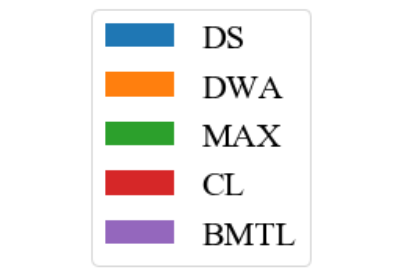
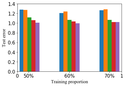
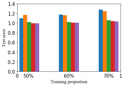
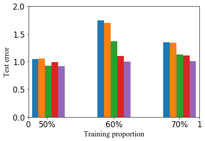
To analyze the effect of the training proportion to the performance, we evaluate the classification accuracy of all the methods by using the training proportion as 50%, 60%, and 70%, respectively, and plot the average test accuracy of all the balancing strategies applied to all the multi-task learning methods in Figures 1-3. Each experimental setting repeats five times and for clear presentation, Figures 1-3 only contain the average accuracies.
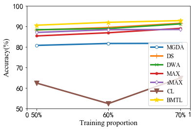
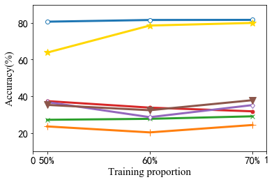
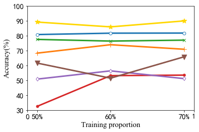
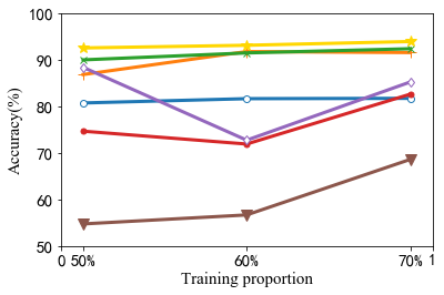
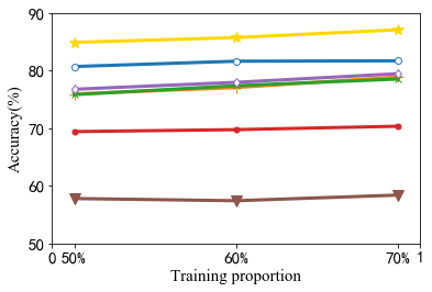
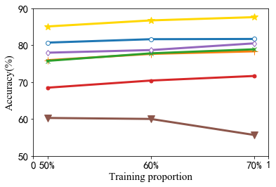
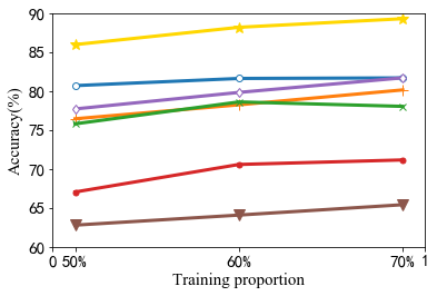
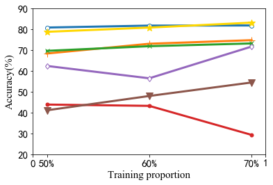
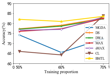
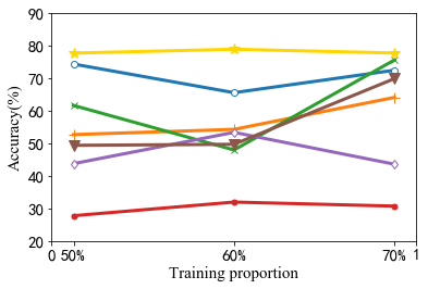
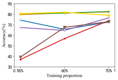
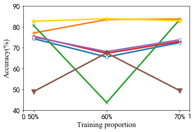
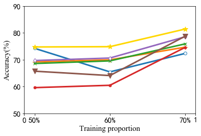
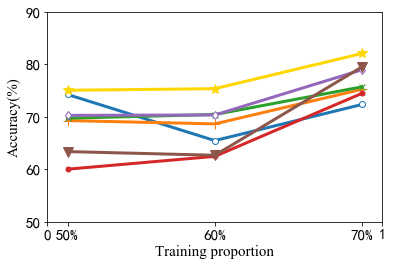
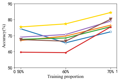
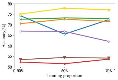
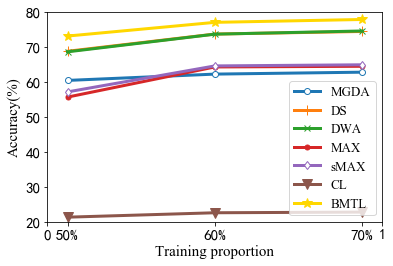
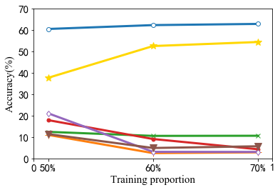
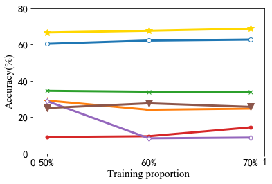
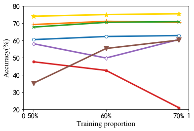
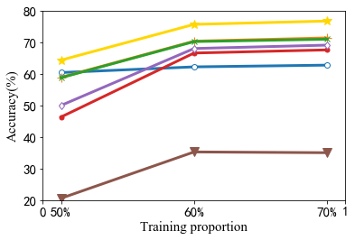
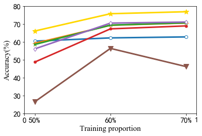
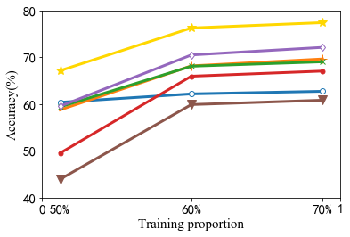
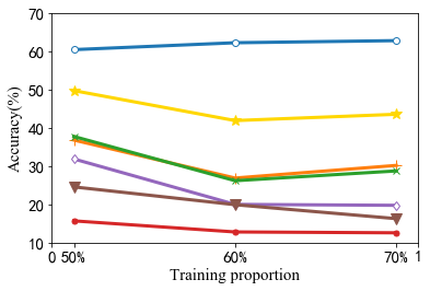
According to Figures 1-3, we can see that when the training proportion increases, the performance of all the balancing strategies on all the multi-task learning models almost improves with some exceptions due to the sensitivity to the initial values for model parameters in multi-task learning models. Moreover, we observe that compared with all the balancing strategies, the proposed BMTL framework improves every multi-task baseline method with different training proportions, which proves the effectiveness and robustness of the BMTL framework.
From the results shown in Figure 1(b), 3(b) and 3(h), we can see that the MGDA method outperforms other losses balancing strategies that are based on the DMTRL_Tucker and MRN methods. One reason is that the MGDA method is specific to the DMTL method and inapplicable to other DMTL methods and hence the comparison here is not so fair. In those settings, the proposed BMTL framework still significantly boosts the performance of the DMTRL_Tucker and MRN methods.
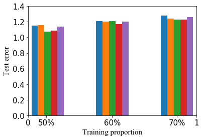
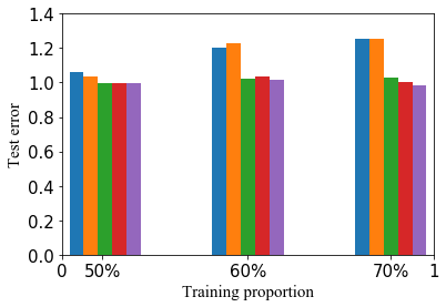
For the SARCOS dataset, we use the mean square error as the performance measure. The results are shown in Figure 5. As shown in Figure 5, the proposed BMTL framework outperforms other balancing strategies, especially based on the TNRMTL methods, which demonstrates the effectiveness of the BMTL framework in this dataset.
4.2.1 Analysis on Training Losses
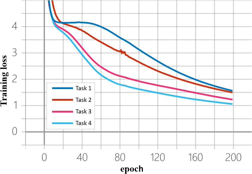
For the proposed BMTL framework based on the DMTRL_TT method, we plot the training losses of different tasks from the Office-Home dataset in Figure 4. From the curves of the training loss, we can observe that tasks with larger training losses draw more attention and decrease faster than other tasks during the training process.
5 Conclusion
In this paper, we propose a balanced multi-task learning framework to handle tasks with unequal difficulty levels. The main idea is to minimize the sum of transformed training losses of all the tasks via the transformation function. The role of the transformation function is to make tasks with larger training losses receive larger weights during the optimization procedure. Some properties of the transformation function are analyzed. Empirical studies conducted on real-world datasets demonstrate the effectiveness of the BMTL framework. In our future work, we will investigate other examples of such as polynomial functions.
References
- Abadi et al. (2016) Abadi, M., Barham, P., Chen, J., Chen, Z., Davis, A., Dean, J., Devin, M., Ghemawat, S., Irving, G., Isard, M., et al. Tensorflow: A system for large-scale machine learning. In Proceedings of the 12th USENIX Symposium on Operating Systems Design and Implementation, pp. 265–283, 2016.
- Ando & Zhang (2005) Ando, R. K. and Zhang, T. A framework for learning predictive structures from multiple tasks and unlabeled data. Journal of Machine Learning Research, 6:1817–1853, 2005.
- Argyriou et al. (2006) Argyriou, A., Evgeniou, T., and Pontil, M. Multi-task feature learning. In Advances in Neural Information Processing Systems 19, pp. 41–48, 2006.
- Bakker & Heskes (2003) Bakker, B. and Heskes, T. Task clustering and gating for bayesian multitask learning. Journal of Machine Learning Research, 4:83–99, 2003.
- Bengio et al. (2009) Bengio, Y., Louradour, J., Collobert, R., and Weston, J. Curriculum learning. In Proceedings of the 26th International Conference on Machine Learning, pp. 41–48, 2009.
- Bonilla et al. (2007) Bonilla, E., Chai, K. M. A., and Williams, C. Multi-task Gaussian process prediction. In Advances in Neural Information Processing Systems 20, pp. 153–160, Vancouver, British Columbia, Canada, 2007.
- Boyd & Vandenberghe (2004) Boyd, S. and Vandenberghe, L. Convex Optimization. Cambridge University Press, 2004.
- Caruana (1997) Caruana, R. Multitask learning. Machine Learning, 28(1):41–75, 1997.
- Chen et al. (2018) Chen, Z., Badrinarayanan, V., Lee, C., and Rabinovich, A. Gradnorm: Gradient normalization for adaptive loss balancing in deep multitask networks. In Proceedings of the 35th International Conference on Machine Learning, pp. 793–802, 2018.
- Désidéri (2012) Désidéri, J.-A. Multiple-gradient descent algorithm (MGDA) for multiobjective optimization. Comptes Rendus Mathematique, 350(5):313–318, 2012.
- Han & Zhang (2016) Han, L. and Zhang, Y. Multi-stage multi-task learning with reduced rank. In Proceedings of the Thirtieth AAAI Conference on Artificial Intelligence, pp. 1638–1644, 2016.
- Hernández-Lobato & Hernández-Lobato (2013) Hernández-Lobato, D. and Hernández-Lobato, J. M. Learning feature selection dependencies in multi-task learning. In Advances in Neural Information Processing Systems 26, pp. 746–754, 2013.
- Hernández-Lobato et al. (2015) Hernández-Lobato, D., Hernández-Lobato, J. M., and Ghahramani, Z. A probabilistic model for dirty multi-task feature selection. In Proceedings of the 32nd International Conference on Machine Learning, pp. 1073–1082, 2015.
- Jacob et al. (2008) Jacob, L., Bach, F., and Vert, J.-P. Clustered multi-task learning: A convex formulation. In Advances in Neural Information Processing Systems 21, pp. 745–752, 2008.
- Kang et al. (2011) Kang, Z., Grauman, K., and Sha, F. Learning with whom to share in multi-task feature learning. In Proceedings of the 28th International Conference on Machine Learning, pp. 521–528, 2011.
- Kendall et al. (2018) Kendall, A., Gal, Y., and Cipolla, R. Multi-task learning using uncertainty to weigh losses for scene geometry and semantics. In Proceedings of IEEE Conference on Computer Vision and Pattern Recognition, pp. 7482–7491, 2018.
- Kingma & Ba (2014) Kingma, D. P. and Ba, J. Adam: A method for stochastic optimization. arXiv preprint arXiv:1412.6980, 2014.
- Kumar et al. (2010) Kumar, M. P., Packer, B., and Koller, D. Self-paced learning for latent variable models. In Advances in Neural Information Processing Systems 23, pp. 1189–1197, 2010.
- Li et al. (2017) Li, C., Yan, J., Wei, F., Dong, W., Liu, Q., and Zha, H. Self-paced multi-task learning. In Proceedings of the Thirty-First AAAI Conference on Artificial Intelligence, pp. 2175–2181, 2017.
- Lin et al. (2019) Lin, X., Zhen, H., Li, Z., Zhang, Q., and Kwong, S. Pareto multi-task learning. In Advances in Neural Information Processing Systems 32, pp. 12037–12047, 2019.
- Liu et al. (2017) Liu, P., Qiu, X., and Huang, X. Adversarial multi-task learning for text classification. In Proceedings of the 55th Annual Meeting of the Association for Computational Linguistics, pp. 1–10, 2017.
- Liu et al. (2019) Liu, S., Johns, E., and Davison, A. J. End-to-end multi-task learning with attention. In Proceedings of IEEE Conference on Computer Vision and Pattern Recognition, pp. 1871–1880, 2019.
- Long et al. (2017) Long, M., Cao, Z., Wang, J., and Yu, P. S. Learning multiple tasks with multilinear relationship networks. In Advances in Neural Information Processing Systems 30, pp. 1593–1602, 2017.
- Lozano & Swirszcz (2012) Lozano, A. C. and Swirszcz, G. Multi-level lasso for sparse multi-task regression. In Proceedings of the 29th International Conference on Machine Learning, 2012.
- McDiarmid (1989) McDiarmid, C. On the method of bounded differences. Surveys in combinatorics, 141(1):148–188, 1989.
- Mehta et al. (2012) Mehta, N. A., Lee, D., and Gray, A. G. Minimax multi-task learning and a generalized loss-compositional paradigm for MTL. In Advances in Neural Information Processing Systems 25, pp. 2159–2167, 2012.
- Misra et al. (2016) Misra, I., Shrivastava, A., Gupta, A., and Hebert, M. Cross-stitch networks for multi-task learning. In Proceedings of IEEE Conference on Computer Vision and Pattern Recognition, pp. 3994–4003, 2016.
- Murugesan & Carbonell (2017) Murugesan, K. and Carbonell, J. G. Self-paced multitask learning with shared knowledge. In Proceedings of the Twenty-Sixth International Joint Conference on Artificial Intelligence, pp. 2522–2528, 2017.
- Obozinski et al. (2006) Obozinski, G., Taskar, B., and Jordan, M. Multi-task feature selection. Technical report, Department of Statistics, University of California, Berkeley, June 2006.
- Pentina et al. (2015) Pentina, A., Sharmanska, V., and Lampert, C. H. Curriculum learning of multiple tasks. In Proceedings of IEEE Conference on Computer Vision and Pattern Recognition, pp. 5492–5500, 2015.
- Russakovsky et al. (2015) Russakovsky, O., Deng, J., Su, H., Krause, J., Satheesh, S., Ma, S., Huang, Z., Karpathy, A., Khosla, A., Bernstein, M., et al. Imagenet large scale visual recognition challenge. International journal of computer vision, 115(3):211–252, 2015.
- Saenko et al. (2010) Saenko, K., Kulis, B., Fritz, M., and Darrell, T. Adapting visual category models to new domains. In European conference on computer vision, pp. 213–226. Springer, 2010.
- Sener & Koltun (2018) Sener, O. and Koltun, V. Multi-task learning as multi-objective optimization. In Advances in Neural Information Processing Systems 31, pp. 525–536, 2018.
- Simonyan & Zisserman (2014) Simonyan, K. and Zisserman, A. Very deep convolutional networks for large-scale image recognition. arXiv preprint arXiv:1409.1556, 2014.
- Venkateswara et al. (2017) Venkateswara, H., Eusebio, J., Chakraborty, S., and Panchanathan, S. Deep hashing network for unsupervised domain adaptation. In Proceedings of IEEE Conference on Computer Vision and Pattern Recognition, 2017.
- Xue et al. (2007) Xue, Y., Liao, X., Carin, L., and Krishnapuram, B. Multi-task learning for classification with Dirichlet process priors. Journal of Machine Learning Research, 8:35–63, 2007.
- Yang & Hospedales (2017a) Yang, Y. and Hospedales, T. M. Deep multi-task representation learning: A tensor factorisation approach. In Proceedings of the 6th International Conference on Learning Representations, 2017a.
- Yang & Hospedales (2017b) Yang, Y. and Hospedales, T. M. Trace norm regularised deep multi-task learning. In Proceedings of the 6th International Conference on Learning Representations, Workshop Track, 2017b.
- Zhang & Yang (2017) Zhang, Y. and Yang, Q. A survey on multi-task learning. CoRR, abs/1707.08114, 2017.
- Zhang & Yeung (2010) Zhang, Y. and Yeung, D.-Y. A convex formulation for learning task relationships in multi-task learning. In Proceedings of the 26th Conference on Uncertainty in Artificial Intelligence, pp. 733–742, 2010.
- Zhang et al. (2010) Zhang, Y., Yeung, D., and Xu, Q. Probabilistic multi-task feature selection. In Advances in Neural Information Processing Systems 23, pp. 2559–2567, 2010.
- Zhang et al. (2014) Zhang, Z., Luo, P., Loy, C. C., and Tang, X. Facial landmark detection by deep multi-task learning. In Proceedings of the 13th European Conference on Computer Vision, pp. 94–108, 2014.
Appendix
Lemma 1 and Its Proof
Lemma 1
For , we have
Proof. Based on the Taylor expansion of the exponential function, we have
which implies
Based on the Taylor expansion of the exponential function again, can be written as
Define and . It is easy to show that and . For , we have
Since , each term in is no smaller than and we reach the conclusion.
Proof for Theorem 1
Proof. According to the requirement, is monotonically increasing on , implying that its second-order derivative is positive, which is equivalent to the strong convexity of on . is already required to be monotonically increasing. As both and are required to be nonnegative, we only require that and due to their monotonically increasing property.
Proof for Theorem 2
Proof: According to the scalar composition rule in Eq. (3.10) of (Boyd & Vandenberghe, 2004), when is convex with respect to and is convex and monotonically increasing, is convex with respect to and so is , leading to the validity of the first part. If further is convex with respect to , both terms in the objective function of problem (8) is convex with respect to , making the whole problem convex.
Proof for Theorem 3
Proof. Since is a convex function, we can get
When each pair of the training data changes, the random variable can change by no more than due to the boundedness of the loss function . Then by McDiarmid’s inequality (McDiarmid, 1989), we can get
where denotes the probability, and this inequality implies that with probability at least ,
If we have another training set with the same distribution as , then we can bound as
Multiplying the term by Rademacher variables , each of which is an uniform -valued random variable, will not change the expectation since . Furthermore, negating a Rademacher variable does not change its distribution. So we have
Note that is -Lipschitz at where . Due to the monotonic property of the loss function such as the cross-entropy loss and the hinge loss with respect to the first input argument, is also a -Lipschitz function. Then based on properties of the Rademacher compliexity, we can get
Then by combining the above inequalities, we can reach the conclusion.
Proof for Theorem 4
Generalization Bound for Linear Models
Based on Theorem 3, we can analyze specific learning models. Here we consider a linear model where is a matrix with columns each of which defines a learning function for a task as . Here is defined as where denotes the Frobenius norm. For problem (10) with such a linear model, we have the following result.
Theorem 5
When , with probability at least where , we have
Proof. According to Theorem 3, we only need to upper-bound . By defining , we have
where the first inequality is due to the Cauchy-Schwartz inequality, the second inequality holds because of the constraint on , the third inequality is due to the Jensen’s inequality based on the square root function, the fourth inequality holds since the norm of each data point is upper-bounded by 1 and is the average of data points in the th task.