On Layer Normalization in the Transformer Architecture
Abstract
The Transformer is widely used in natural language processing tasks. To train a Transformer however, one usually needs a carefully designed learning rate warm-up stage, which is shown to be crucial to the final performance but will slow down the optimization and bring more hyper-parameter tunings. In this paper, we first study theoretically why the learning rate warm-up stage is essential and show that the location of layer normalization matters. Specifically, we prove with mean field theory that at initialization, for the original-designed Post-LN Transformer, which places the layer normalization between the residual blocks, the expected gradients of the parameters near the output layer are large. Therefore, using a large learning rate on those gradients makes the training unstable. The warm-up stage is practically helpful for avoiding this problem. On the other hand, our theory also shows that if the layer normalization is put inside the residual blocks (recently proposed as Pre-LN Transformer), the gradients are well-behaved at initialization. This motivates us to remove the warm-up stage for the training of Pre-LN Transformers. We show in our experiments that Pre-LN Transformers without the warm-up stage can reach comparable results with baselines while requiring significantly less training time and hyper-parameter tuning on a wide range of applications.
1 Introduction
The Transformer (Vaswani et al., 2017) is one of the most commonly used neural network architectures in natural language processing. Layer normalization (Lei Ba et al., 2016) plays a key role in Transformer’s success. The originally designed Transformer places the layer normalization between the residual blocks, which is usually referred to as the Transformer with Post-Layer Normalization (Post-LN) (Wang et al., 2019). This architecture has achieved state-of-the-art performance in many tasks including language modeling (Dai et al., 2019; Al-Rfou et al., 2018) and machine translation (Dehghani et al., 2018; Edunov et al., 2018). Unsupervised pre-trained models based on the Post-LN Transformer architecture also show impressive performance in many downstream tasks (Radford et al., 2019; Devlin et al., 2018; Yang et al., 2019b).
Despite its great success, people usually need to deal with the optimization of the Post-LN Transformer more carefully than convolutional networks or other sequence-to-sequence models (Popel & Bojar, 2018). In particular, to train the model from scratch, any gradient-based optimization approach requires a learning rate warm-up stage (Vaswani et al., 2017; Liu et al., 2019a): the optimization starts with an extremely small learning rate, and then gradually increases it to a pre-defined maximum value in a pre-defined number of iterations. Such a warm-up stage not only slows down the optimization process but also brings more hyperparameter tunings. Popel & Bojar (2018) has shown that the final model performance is quite sensitive to the value of the maximum learning rate and the number of warm-up iterations. Tuning such sensitive hyper-parameters is costly in training large-scale models, e.g., BERT (Devlin et al., 2018) or XLNet (Yang et al., 2019b).
In this paper, we try to alleviate this problem by finding ways to safely remove the learning rate warm-up stage. As the warm-up stage happens in the first several iterations, we investigate the optimization behavior at initialization using mean field theory (Lee et al., 2017; Xiao et al., 2018; Yang et al., 2019a; Yang, 2019; Lee et al., 2019; Zhang et al., 2019). According to our theoretical analysis, when putting the layer normalization between the residual blocks, the expected gradients of the parameters near the output layer are large. Therefore, without the warm-up stage, directly using a large learning rate to those parameters can make the optimization process unstable. Using a warm-up stage and training the model with small learning rates practically avoid this problem. Extensive experiments are provided to support our theoretical findings.
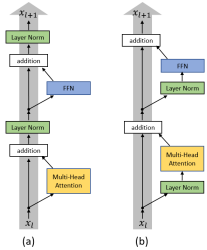
Our theory also shows that the layer normalization plays a crucial role in controlling the gradient scales. This motivates us to investigate whether there are some other ways of positioning the layer normalization that lead to well-behaved gradients. In particular, we study another variant, the Transformer with Pre-Layer Normalization (Pre-LN) (Baevski & Auli, 2018; Child et al., 2019; Wang et al., 2019). The Pre-LN Transformer puts the layer normalization inside the residual connection and equips with an additional final-layer normalization before prediction (Please see Figure 1 for the differences between the two variants of the Transformer architectures). We show that at initialization, the gradients are well-behaved without any exploding or vanishing for the Pre-LN Transformer both theoretically and empirically.
Given the gradients are well-behaved in the Pre-LN Transformer, it is natural to consider removing the learning rate warm-up stage during training. We conduct a variety of experiments, including IWSLT14 German-English translation, WMT14 English-German translation, and BERT pre-training tasks. We show that, in all tasks, the learning rate warm-up stage can be safely removed, and thus, the number of hyper-parameter is reduced. Furthermore, we observe that the loss decays faster for the Pre-LN Transformer model. It can achieve comparable final performances but use much less training time. This is particularly important for training large-scale models on large-scale datasets.
Our contributions are summarized as follows:
We investigate two Transformer variants, the Post-LN Transformer and the Pre-LN Transformer, using mean field theory. By studying the gradients at initialization, we provide evidence to show why the learning rate warm-up stage is essential in training the Post-LN Transformer.
We are the first to show that the learning-rate warm-up stage can be removed for the Pre-LN Transformer, which eases the hyperparameter tuning. We further show that by using proper learning rate schedulers, the training time can be largely reduced on a wide range of applications.
2 Related work
Gradient descent-based methods (Kingma & Ba, 2014; Zeiler, 2012; Duchi et al., 2011; Tieleman & Hinton, 2012) are popularly used in optimizing deep neural networks. For convolutional neural networks and recurrent neural networks, a relatively large learning rate is usually set in the beginning, and then decreased along with the optimization process (He et al., 2016, 2017; Sutskever et al., 2014; Gehring et al., 2017; He et al., 2019). The learning rate warm-up stage has only been shown essential in dealing with some very specific problems, e.g., the large-batch training. Goyal et al. (2017); He et al. (2019); You et al. (2018) showed that a learning rate warm-up stage is preferred when training neural networks with extremely large batch sizes.
However, the learning rate warm-up stage is essential and critical when optimizing the Transformer models in a majority of scenarios (Vaswani et al., 2017; Devlin et al., 2018; Dai et al., 2019; Radford et al., 2019; Lu et al., 2019). Popel & Bojar (2018) investigated the influence of different warm-up strategies for the optimization of the Post-LN Transformer model and found that without or with relatively less warm-up iterations, the optimization diverges. The Pre-LN Transformer has been proposed in several recent works (Baevski & Auli, 2018; Child et al., 2019; Wang et al., 2019) to alleviate some optimization issues when training deeper models, but the troublesome warm-up stage still remains in their training pipelines.
(Liu et al., 2019a) claimed that the benefit of the warm-up stage comes from reducing the variance for the adaptive learning rate in the Adam optimizer (Kingma & Ba, 2014). They proposed to rectify the variance of adaptive learning rate by a new variant of Adam called RAdam. However, we find that not only for Adam, the learning rate warm-up stage also helps quite a lot for other optimizers. This may indicate that Adam is not the prerequisite for the necessity of the warm-up stage. In a concurrent and independent work, Nguyen & Salazar (2019) also empirically observed that the Pre-LN Transformer can be trained without learning rate warm-up stage. Our work provides a more comprehensive study regrading this with a theoretical analysis.
3 Optimization for the Transformer
3.1 Transformer with Post-Layer Normalization
The Transformer architecture usually consists of stacked Transformer layers (Vaswani et al., 2017; Devlin et al., 2018), each of which takes a sequence of vectors as input and outputs a new sequence of vectors with the same shape. A Transformer layer has two sub-layers: the (multi-head) self-attention sub-layer and the position-wise feed-forward network sub-layer. Residual connection (He et al., 2016) and layer normalization (Lei Ba et al., 2016) are applied for both sub-layers individually. We first introduce each component of the Transformer layer and then present the entire architecture.
Self-attention sub-layer
An attention function can be formulated as querying an entry with key-value pairs (Vaswani et al., 2017). The self-attention sub-layer uses scaled dot-product attention, which is defined as: , where is the dimensionality of the hidden representations, and (Query), (Key), (Value) are specified as the hidden representations of the previous layer. The multi-head variant of the self-attention sub-layer is popularly used which allows the model to jointly attend to information from different representation sub-spaces, and is defined as
where and are project parameter matrices, is the number of heads. and are the dimensionalities of Key and Value. Without any confusion, given a sequence of vectors , we use as the multi-head self-attention mechanism on position which considers the attention from to the entire sequence, i.e., .
Position-wise FFN sub-layer
In addition to the self-attention sub-layer, each Transformer layer contains a fully connected network, which is applied to each position separately and identically. This sub-layer is a two-layer feed-forward network with a ReLU activation function. Given a sequence of vectors , the computation of a position-wise FFN sub-layer on any is defined as:
where , , and are parameters.
Residual connection and layer normalization
Besides the two sub-layers described above, the residual connection and layer normalization are also key components to the Transformer. For any vector , the layer normalization is computed as , in which are the mean and standard deviation of the elements in , i.e., and . Scale and bias vector are parameters.
Different orders of the sub-layers, residual connection and layer normalization in a Transformer layer lead to variants of Transformer architectures. One of the original and most popularly used architecture for the Transformer and BERT (Vaswani et al., 2017; Devlin et al., 2018) follows “self-attention (FFN) sub-layer residual connection layer normalization”, which we call the Transformer with Post-Layer normalization (Post-LN Transformer), as illustrated in Figure 1.
Post-LN Transformer
Denote as the input of the -th Transformer layer at position , where is a real-valued vector of dimension , , . is the length of the sequence and is the number of layers. For completeness, we define as the input embedding at position which is usually a combination of word embedding and positional embedding. The computations inside the -th layer are composed of several steps, and we use super-scripts on to present the input(output) of different steps as in Table 1 (left), where , , and are parameters of the FFN sub-layer in the -th layer.
Post-LN Transformer Pre-LN Transformer Final LayerNorm:
3.2 The learning rate warm-up stage
We are interested in the learning rate warm-up stage in the optimization of the Post-LN Transformer. Different from the optimization of many other architectures in which the learning rate starts from a relatively large value and then decays (Bahdanau et al., 2017; Dauphin et al., 2017), a learning rate warm-up stage for the Post-LN Transformer seems critical (Popel & Bojar, 2018). We denote the learning rate of the -th iteration as and the maximum learning rate during training as . Given a predefined time frame , the learning rate scheduler for the first iterations (Vaswani et al., 2018) is defined as
| (1) |
After this warm-up stage, the learning rate will be set by classical learning rate schedulers, such as the linear decay, the inverse square-root decay, or forced decay at particular iterations. We conduct experiments to show that this learning rate warm-up stage is essential for training Post-LN Transformer models.
Experimental setting
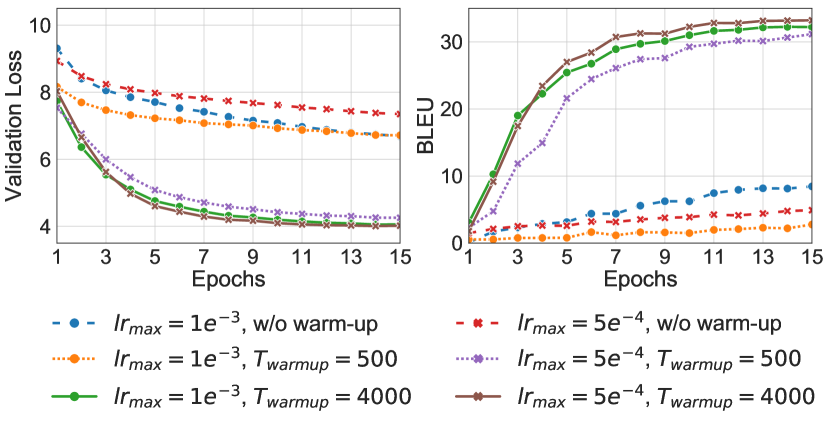
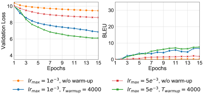
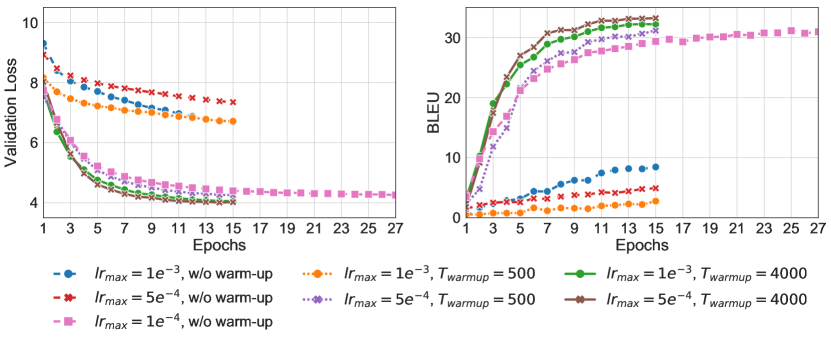
We conduct experiments on the IWSLT14 German-to-English (De-En) machine translation task. We mainly investigate two aspects: whether the learning rate warm-up stage is essential and whether the final model performance is sensitive to the value of . To study the first aspect, we train the model with the Adam optimizer (Kingma & Ba, 2014) and the vanilla SGD optimizer (Ruder, 2016) respectively. For both optimziers, we check whether the warm-up stage can be removed. We follow Vaswani et al. (2017) to set hyper-parameter to be in Adam. We also test different for both optimizers. For Adam, we set or , and for SGD, we set or . When the warm-up stage is used, we set as suggested by the original paper (Vaswani et al., 2017). To study the second aspect, we set to be 1/500/4000 (“1” refers to the no warm-up setting) and use or with Adam. For all experiments, a same inverse square root learning rate scheduler is used after the warm-up stage. We use both validation loss and BLEU (Papineni et al., 2002) as the evaluation measure of the model performance.
Results and discussions
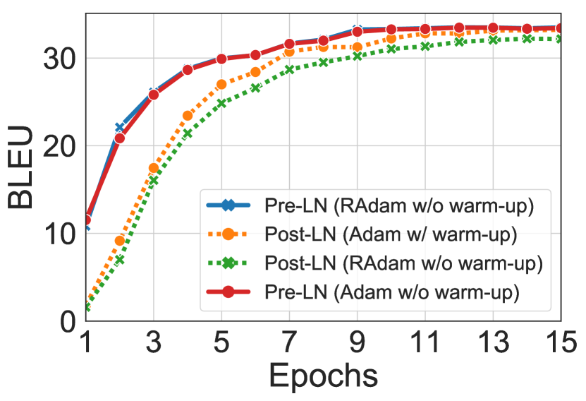
We record the model checkpoints for every epoch during training and calculate the validation loss and BLEU score. The performance of the models are plotted in Figure 2(a) and Figure 2(b). The x-axis is the epoch number and the y-axis is the BLEU score/validation loss. "w/o warm-up" indicates “without the warm-up stage” while "w/ warm-up" indicates “with the warm-up stage”.
First, we can see that for both optimizers, the learning rate warm-up stage is essential. Without the warm-up stage, the BLEU score of the model trained with Adam optimizer can only achieve 8.45. As a comparison, the model trained using the warm-up stage can achieve around 34 in terms of BLEU score. The same trend can also be observed on the validation loss curves. Although the performance of the model trained with SGD is significantly worse than Adam, we can still see similar phenomena as Adam. The BLEU score is just above zero in 15 epochs without using the warm-up stage.
Second, we can see that the optimization process is sensitive to the value of , which means is an important hyper-parameter in training the Post-LN Transformer. For example, when setting , the learned models with Adam achieve only 31.16 and 2.77 in term of BLEU score for and respectively.
Such a warm-up stage has several disadvantages. First, its configuration significantly affects the final performance. The practitioners need a careful hyper-parameter tuning, which is computationally expensive for large-scale NLP tasks. Second, the warm-up stage could slow down the optimization. Standard optimization algorithms usually start with a large learning rate for fast convergence. However, when using the warm-up stage, the learning rate has to gradually increase from zero, which may make the training inefficient. Liu et al. (2019a) suggests that the warm-up stage plays a role in reducing the undesirably significant variance in Adam in the early stage of model training. However, according to our results, the warm-up stage also helps the training of SGD. This suggests that the benefit of the warm-up stage may be not for a particular optimizer.
3.3 Understanding the Transformer at initialization
We can see that the Post-LN Transformer cannot be trained with a large learning rate from scratch. This motivates us to investigate what happens at the model initialization. We first introduce the parameter initialization setting for our theoretical analysis and then present our theoretical findings.
Notations
We denote as the loss function of one position, as the loss function of the whole sequence, and as the norm (spectral norm) and the Frobenius norm, as the standard layer normalization with scale and bias , and as the Jacobian matrix of . Let denote standard Big-O notation that suppress multiplicative constants.
Parameter Initialization
The parameter matrices in each Transformer layer are usually initialized by the Xavier initialization (Glorot & Bengio, 2010). Given a matrix of size , the Xavier initialization sets the value of each element by independently sampling from Gaussian distribution . The bias vectors are usually initialized as zero vectors. The scale in the layer normalization is set to one.
For theoretical analysis, we study a simpler setting. First, we focus on single-head attention instead of the multi-head variant and for all layers, we set the shape of , , , , to be . Second, we initialize the parameter matrices in the self-attention sub-layer and to be zero matrices. In this setting, the attention is a uniform distribution at initialization and can be simplified as . Third, we assume the input vectors are also sampled from the same Gaussian distribution. This is reasonable since the inputs are linear combinations of word embeddings and learnable positional embeddings, both of which are initialized by Gaussian distributions.
Post-LN Transformer v.s. Pre-LN Transformer
We compare the Post-LN Transformer with another variant of the Transformer architecture, the Transformer with Pre-Layer Normalization (Pre-LN). The Pre-LN Transformer was implemented in several systems (Vaswani et al., 2018; Klein et al., 2018; Liu et al., 2019b). Wang et al. (2019) suggested that the Pre-LN Transformer outperforms the Post-LN Transformer when the number of layers increases. Different from the Post-LN Transformer that puts the layer normalization between the residual blocks, the Pre-LN Transformer puts the layer normalization inside the residual connection and places it before all other non-linear transformations. Additionally, the Pre-LN Transformer uses a final layer normalization right before the prediction. We provide the mathematical formulations and visualizations of the Post-LN/Pre-LN Transformer in Table 1 and Figure 1.
For both architectures, each passes through a softmax layer to produce a distribution over the dictionary . The loss function is defined on the softmax distribution. For example, in sequence prediction, the loss function is defined as for the Post-LN Transformer and for the Pre-LN Transformer, where is the probability of ground truth token outputted by the softmax distribution and is the word embedding matrix. The loss of the whole sequence is an average of the loss on each position. Without loss of generality, we assume that all the derivatives are bounded. We introduce the following concentration property of random variables which will be further used in the theorem.
Definition 1.
A random variable is called -bounded if with probability at least , , where and .
Intuitively, if the random variable is -bounded, then with a high probability its realization will not get too far away from its expectation. For example, if is a -dimensional standard Gaussian random vector, then is -bounded with , (see supplementary material for details). As parameter matrices in self-attention sub-layers and FFN sub-layers are initialized by Gaussian distributions, if the norm of the hidden states in the Transformer satisfies the concentrated condition above, we have the following theorem to characterize the scale of the gradients.
Theorem 1 (Gradients of the last layer in the Transformer).
Assume that and are -bounded for all , where and are small numbers. Then with probability at least , for the Post-LN Transformer with layers, the gradient of the parameters of the last layer satisfies
and for the Pre-LN Transformer with layers,
From Theorem 1, we can see that for the Post-LN Transformer, the scale of the gradients to the last FFN layer is of order which is independent of . For the Pre-LN Transformer, the scale of the gradients is much smaller. We first study the forward propagation of the Post-LN Transformer and the Pre-LN Transformer. Lemma 1 will be served as a basic tool to prove the main theorem and other lemmas.
Lemma 1.
If is a Gaussian vector, , then .
Based on Lemma 1, we have the following lemma to estimate the scale of the hidden states in different layers for the Post-LN Transformer and the Pre-LN Transformer.
Lemma 2.
At initialization, for the Post-LN Transformer, for all and . For the Pre-LN Transformer, for all and . Expectations are taken over the input and the randomness of initialization.
Lemma 2 studies the expected norm of the hidden states in both Post-LN/Pre-LN Transformer. It is obviously that in the Post-LN Transformer, the norm of is and thus we study the norm of instead. As we can see from Lemma 2, the scale of the hidden states in the Post-LN Transformer keeps to be the same in expectation while the scale of the hidden states in the Pre-LN Transformer grows linearly along with the depth. The next lemma shows that the scale of the hidden states highly relates to the scale of the gradient in the architectures using layer normalization.
Lemma 3.
For , we have in which .
The proof of Lemma 1, Lemma 2, Lemma 3, and Theorem 1 can be found in the supplementary material. The main idea is that the layer normalization will normalize the gradients. In the Post-LN Transformer, the scale of the inputs to the layer normalization is independent of , and thus the gradients of parameters in the last layer are independent of . While in the Pre-LN Transformer, the scale of the input to the final layer normalization is linear in , and thus the gradients of all parameters will be normalized by .
Extended theory to other layers/parameters
We have provided a formal proof on the gradients of the last FFN sub-layer as above. In order to fully understand the optimization, we also make some preliminary analysis for other layers and other parameters. Our main result is that the gradient norm in the Post-LN Transformer is large for the parameters near the output and will be likely to decay as the layer index decreases. On the contrary, the gradient norm in the Pre- Transformer will be likely to stay the same for any layer . All the preliminary theoretical results are provided in the supplementary material.
3.4 Empirical verification of the theory and discussion
As our theory is derived based on several simplifications of the problem, we conduct experiments to study whether our theoretical insights are consistent with what we observe in real scenarios. The general model and training configuration exactly follow Section 3.2. The experiments are repeated ten times using different random seeds.
On the concentration property
Given an initialized model, we record the hidden states in the Post-LN/Pre-LN Transformer across batches and find that the norm of the hidden states satisfies the property ((0.1,0.125)-bounded).
On Theorem 1
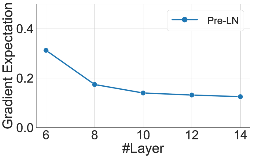
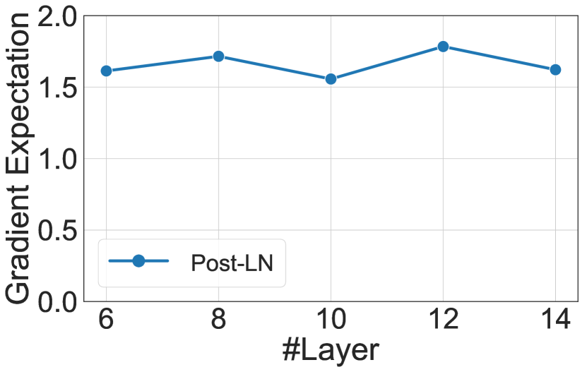
Theorem 1 suggests that for any sizes of the Post-LN Transformer, the scale of the gradient norm in the last FFN sub-layer remains the same. On the contrary, that of the Pre-LN Transformer decreases as the size of the model grows. We calculate and record the gradient norm in the last FFN sub-layer in 6-6/8-8/10-10/12-12/14-14 Post-LN/Pre-LN Transformer models at initialization. The results are plotted in Figure 3(c) and 3(d). The x-axis is the size of the model, and the y-axis is the value of the gradient norm of in the final FFN sub-layer. The figures show when the number of layers grows, the gradient norm remains in the Post-LN Transformer (around 1.6) and decreases in the Pre-LN Transformer. This observation is consistent with our theory.
On the extended theory
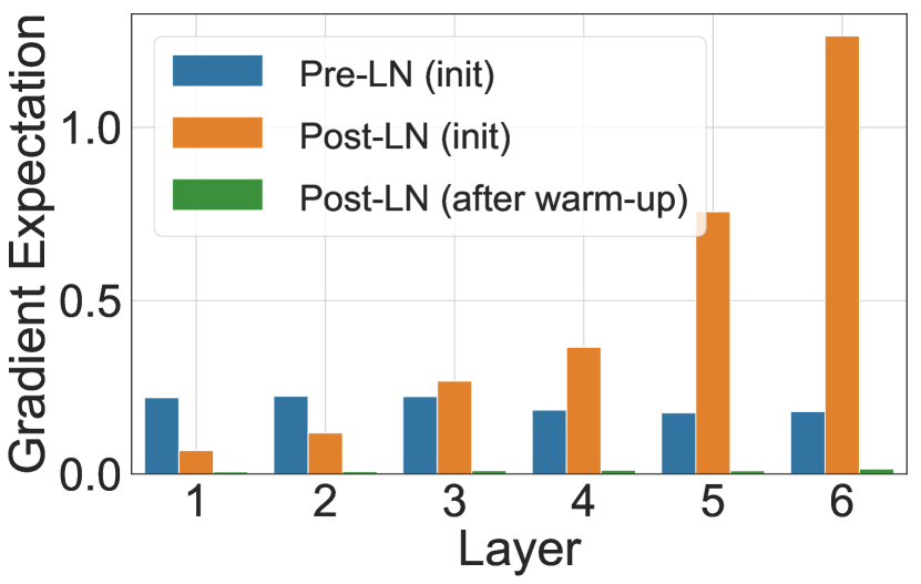
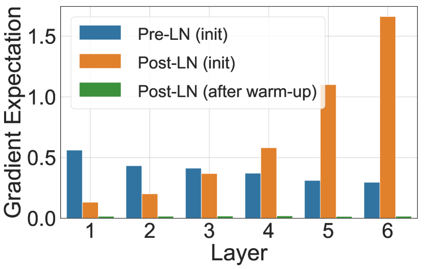
We calculate the gradient norm of each paramter matrix in 6-6 Post-LN/Pre-LN Transformer. We record the gradient for each parameter for different mini-batches. For elements in a parameter matrix, we calculate their expected gradients and use the Frobenius norm of those values as the scale of the expected gradient of the matrix. Figure 3(a) and 3(b) shows those statistics for FFN sub-layers. The x-axis indexes different Transformer layers. It can be seen from the figure, the scale of the expected gradients grows along with the layer index for the Post-LN Transformer. On the contrary, the scale almost keeps the same for different layers in the Pre-LN Transformer. These observations are consistent with our theoretical findings.
The critical warm-up stage for Post-LN Transformer
Given the analysis above, we hypothesize that the gradient scale is one of the reasons that the Post-LN Transformer needs a careful learning rate scheduling. Since the gradients are large for some layers, using a large learning rate without warm-up may make the training unstable.
To verify this argument, first, we study the gradient statistics for the Post-LN Transformer after the warm-up stage with Adam. It can be seen from Figure 3(a) and 3(b) that the scale of the gradients are very small, and the model can be trained with large learning rates. Second, we conduct an experiment to train the Post-LN Transformer from scratch using a fixed small learning rate, i.e., , to verify whether using small-step updates mitigates the issue. The details are provided in the supplementary material. In general, using a very small and fixed learning rate can mitigate the problem and optimize the Post-LN Transformer to a certain extent but the convergence is significantly slower. Both experiments above are supportive to our claim.
4 Experiments
We find in the previous section that the gradients at initialization for Pre-LN Transformer are well-behaved. Given this observation, we deduce that the learning rate warm-up stage can be safely removed when training Pre-LN Transformer. In this section, we empirically verify it on two main tasks in NLP, machine translation and unsupervised pre-training.
4.1 Experiment Settings
Machine Translation
We conduct our experiments on two widely used tasks: the IWSLT14 German-to-English (De-En) task and the WMT14 English-to-German (En-De) task. For the IWSLT14 De-En task, we use the same model configuration as in Section 3. For the WMT14 En-De task, we use the Transformer base setting. More details can be found in the supplementary material.
For training the Pre-LN Transformer, we remove the learning rate warm-up stage. On the IWSLT14 De-En task, we set the initial learning rate to be and decay the learning rate at the 8-th epoch by 0.1. On the WMT14 En-De task, we run two experiments in which the initial learning rates are set to be respectively. Both learning rates are decayed at the 6-th epoch followed by the inverse square root learning rate scheduler.
We train the Post-LN Transformer using the learning rate warm-up stage as the baseline. In both IWSLT14 De-En task and WMT14 En-De task, we set the number of the warm-up stage to be 4000 following Vaswani et al. (2017) and then use the inverse square root learning rate scheduler. For all experiments above, we use the Adam optimizer and set the hyper-parameter to be . We set as same as the initial learning rates of the Pre-LN Transformer in each corresponding experiment. Since Liu et al. (2019a) suggests that the learning rate warm-up stage can be removed using RAdam, we try this optimizer on the IWSLT14 De-En task. We use linear learning rate decay suggested by Liu et al. (2019a) and keep all other hyper-parameters to be the same as in other experiments.
Unsupervised Pre-training (BERT)
We follow (Devlin et al., 2018) to use English Wikipedia corpus and BookCorpus for pre-training. As the dataset BookCorpus (Zhu et al., 2015) is no longer freely distributed. We follow the suggestions from (Devlin et al., 2018) to crawl and collect BookCorpus on our own. The concatenation of two datasets contains roughly 3.4B words in total, which is comparable with the data corpus used in (Devlin et al., 2018). We randomly split documents into one training set and one validation set. The training-validation ratio for pre-training is 199:1.
We use base model configuration in our experiments. Similar to the translation task, we train the Pre-LN BERT without the warm-up stage and compare it with the Post-LN BERT. We follow the same hyper-parameter configuration in Devlin et al. (2018) to train the Post-LN BERT using 10k warm-up steps with . For the Pre-LN BERT, we use linear learning rate decay starting from without the warm-up stage. We have tried to use a larger learning rate (such as ) for the Post-LN BERT but found the optimization diverged.
4.2 Experiment Results
Machine Translation
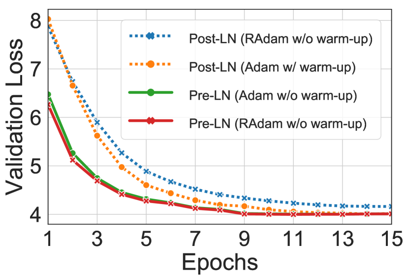
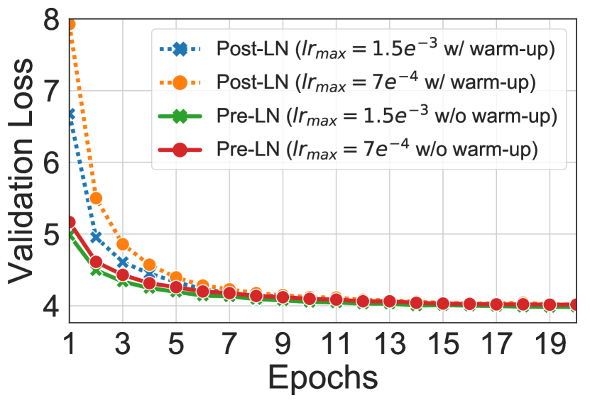
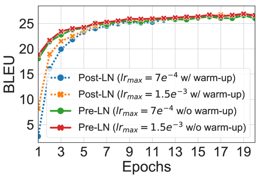
We record the model checkpoints for every epoch during training and calculate the validation loss and BLEU score. The performance of the models at different checkpoints are plotted in Figure 4(a) - 4(d).
First, as we can see from the figure, the learning rate warm-up stage is not critical anymore for training the Pre-LN Transformer and the performance of the learned model is competitive. For example, on the IWSLT14 De-En task, the BLEU score and validation loss of the Pre-LN Transformer can achieve around 34 and 4, which are comparable with the performance of the Post-LN Transformer.
Second, the Pre-LN Transformer converges faster than the Post-LN Transformer using the same . On the IWSLT14 De-En task, the 9-th checkpoint of the Pre-LN Transformer achieves nearly the same performance (validation loss/BLEU score) as 15-th checkpoint of the Post-LN Transformer. Similar observations can be found in the WMT14 En-De task.
Third, compared with RAdam, we find that the change of the position of layer normalization “dominates” the change of the optimizer. According to our experiments on the IWSLT14 De-En task, we can see that although RAdam trains the Post-LN Transformer well without the warm-up stage, it has little difference with Adam when training the Pre-LN Transformer.
Unsupervised Pre-training (BERT)
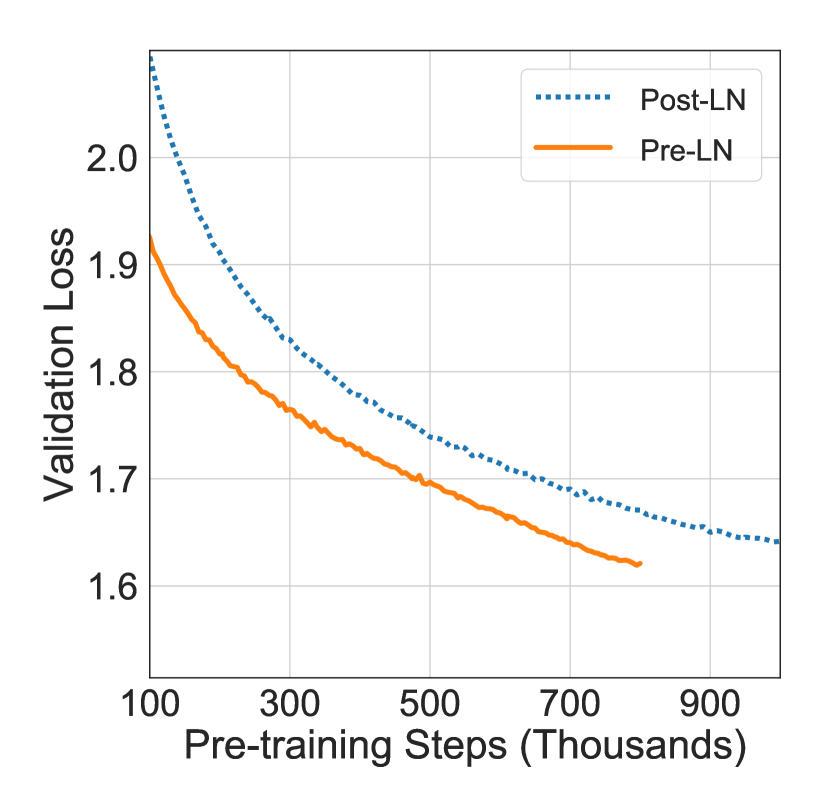
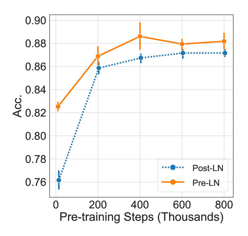
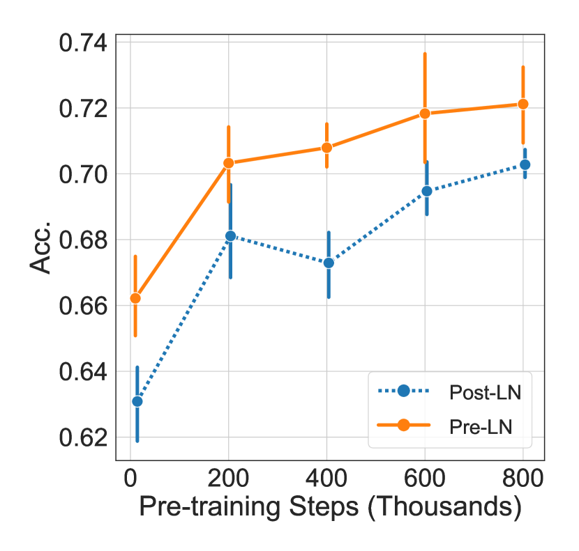
We record validation loss of the model checkpoints and plot them in Figure 5(a). Similar to the machine translation tasks, the learning rate warm-up stage can be removed for the Pre-LN model. The Pre-LN model can be trained faster. For example, the Post-LN model achieves 1.69 validation loss at 500k updates while the Pre-LN model achieves similar validation loss at 700k updates, which suggests there is a 40% speed-up rate. Note that (10k) is far less than the acceleration (200k) which suggests the Pre-LN Transformer is easier to optimize using larger learning rates. We also evaluate different model checkpoints on the downstream task MRPC and RTE (more details can be found in the supplementary material). The experiments results are plotted in Figure 5(b) and 5(c). We can see that the Pre-LN model also converges faster on the downstream tasks.
As a summary, all the experiments on different tasks show that training the Pre-LN Transformer does not rely on the learning rate warm-up stage and can be trained much faster than the Post-LN Transformer.
5 Conclusion and Future Work
In this paper, we study why the learning rate warm-up stage is important in training the Transformer and show that the location of layer normalization matters. We show that in the original Transformer, which locates the layer normalization outside the residual blocks, the expected gradients of the parameters near the output layer are large at initialization. This leads to an unstable training when using a large learning rate. We further show that the Transformer which locates the layer normalization inside the residual blocks, can be trained without the warm-up stage and converges much faster. In the future, we will investigate other strategies of positioning the layer normalization and understand the optimization of Transformer from a theoretical perspective.
References
- Al-Rfou et al. (2018) Al-Rfou, R., Choe, D., Constant, N., Guo, M., and Jones, L. Character-level language modeling with deeper self-attention. arXiv preprint arXiv:1808.04444, 2018.
- Baevski & Auli (2018) Baevski, A. and Auli, M. Adaptive input representations for neural language modeling. arXiv preprint arXiv:1809.10853, 2018.
- Bahdanau et al. (2017) Bahdanau, D., Cho, K., and Bengio, Y. Neural machine translation by jointly learning to align and translate. 2017.
- Bentivogli et al. (2009) Bentivogli, L., Dagan, I., Dang, H. T., Giampiccolo, D., and Magnini, B. The fifth PASCAL recognizing textual entailment challenge. 2009.
- Child et al. (2019) Child, R., Gray, S., Radford, A., and Sutskever, I. Generating long sequences with sparse transformers. arXiv preprint arXiv:1904.10509, 2019.
- Dai et al. (2019) Dai, Z., Yang, Z., Yang, Y., Cohen, W. W., Carbonell, J., Le, Q. V., and Salakhutdinov, R. Transformer-xl: Attentive language models beyond a fixed-length context. arXiv preprint arXiv:1901.02860, 2019.
- Dauphin et al. (2017) Dauphin, Y. N., Fan, A., Auli, M., and Grangier, D. Language modeling with gated convolutional networks. In International Conference on Machine Learning, pp. 933–941, 2017.
- Dehghani et al. (2018) Dehghani, M., Gouws, S., Vinyals, O., Uszkoreit, J., and Kaiser, Ł. Universal transformers. arXiv preprint arXiv:1807.03819, 2018.
- Devlin et al. (2018) Devlin, J., Chang, M.-W., Lee, K., and Toutanova, K. Bert: Pre-training of deep bidirectional transformers for language understanding. arXiv preprint arXiv:1810.04805, 2018.
- Dolan & Brockett (2005) Dolan, W. B. and Brockett, C. Automatically constructing a corpus of sentential paraphrases. In Proceedings of the International Workshop on Paraphrasing., 2005.
- Duchi et al. (2011) Duchi, J., Hazan, E., and Singer, Y. Adaptive subgradient methods for online learning and stochastic optimization. Journal of Machine Learning Research, 12(Jul):2121–2159, 2011.
- Edunov et al. (2018) Edunov, S., Ott, M., Auli, M., and Grangier, D. Understanding back-translation at scale. arXiv preprint arXiv:1808.09381, 2018.
- Gehring et al. (2017) Gehring, J., Auli, M., Grangier, D., Yarats, D., and Dauphin, Y. N. Convolutional sequence to sequence learning. In International Conference on Machine Learning, pp. 1243–1252, 2017.
- Glorot & Bengio (2010) Glorot, X. and Bengio, Y. Understanding the difficulty of training deep feedforward neural networks. In Proceedings of the thirteenth international conference on artificial intelligence and statistics, pp. 249–256, 2010.
- Goyal et al. (2017) Goyal, P., Dollár, P., Girshick, R., Noordhuis, P., Wesolowski, L., Kyrola, A., Tulloch, A., Jia, Y., and He, K. Accurate, large minibatch sgd: Training imagenet in 1 hour. arXiv preprint arXiv:1706.02677, 2017.
- He et al. (2016) He, K., Zhang, X., Ren, S., and Sun, J. Deep residual learning for image recognition. In Proceedings of the IEEE conference on computer vision and pattern recognition, pp. 770–778, 2016.
- He et al. (2017) He, K., Gkioxari, G., Dollár, P., and Girshick, R. Mask r-cnn. In Proceedings of the IEEE international conference on computer vision, pp. 2961–2969, 2017.
- He et al. (2019) He, T., Zhang, Z., Zhang, H., Zhang, Z., Xie, J., and Li, M. Bag of tricks for image classification with convolutional neural networks. In Proceedings of the IEEE Conference on Computer Vision and Pattern Recognition, pp. 558–567, 2019.
- Kingma & Ba (2014) Kingma, D. P. and Ba, J. Adam: A method for stochastic optimization. arXiv preprint arXiv:1412.6980, 2014.
- Klein et al. (2018) Klein, G., Kim, Y., Deng, Y., Nguyen, V., Senellart, J., and Rush, A. Opennmt: Neural machine translation toolkit. In Proceedings of the 13th Conference of the Association for Machine Translation in the Americas (Volume 1: Research Papers), volume 1, pp. 177–184, 2018.
- Koehn et al. (2007) Koehn, P., Hoang, H., Birch, A., Callison-Burch, C., Federico, M., Bertoldi, N., Cowan, B., Shen, W., Moran, C., Zens, R., et al. Moses: Open source toolkit for statistical machine translation. In Proceedings of the 45th annual meeting of the association for computational linguistics companion volume proceedings of the demo and poster sessions, pp. 177–180, 2007.
- Lee et al. (2017) Lee, J., Bahri, Y., Novak, R., Schoenholz, S. S., Pennington, J., and Sohl-Dickstein, J. Deep neural networks as gaussian processes. arXiv preprint arXiv:1711.00165, 2017.
- Lee et al. (2019) Lee, J., Xiao, L., Schoenholz, S. S., Bahri, Y., Sohl-Dickstein, J., and Pennington, J. Wide neural networks of any depth evolve as linear models under gradient descent. arXiv preprint arXiv:1902.06720, 2019.
- Lei Ba et al. (2016) Lei Ba, J., Kiros, J. R., and Hinton, G. E. Layer normalization. arXiv preprint arXiv:1607.06450, 2016.
- Liu et al. (2019a) Liu, L., Jiang, H., He, P., Chen, W., Liu, X., Gao, J., and Han, J. On the variance of the adaptive learning rate and beyond. arXiv preprint arXiv:1908.03265, 2019a.
- Liu et al. (2019b) Liu, Y., Ott, M., Goyal, N., Du, J., Joshi, M., Chen, D., Levy, O., Lewis, M., Zettlemoyer, L., and Stoyanov, V. Roberta: A robustly optimized bert pretraining approach. arXiv preprint arXiv:1907.11692, 2019b.
- Lu et al. (2019) Lu, Y., Li, Z., He, D., Sun, Z., Dong, B., Qin, T., Wang, L., and Liu, T.-Y. Understanding and improving transformer from a multi-particle dynamic system point of view. arXiv preprint arXiv:1906.02762, 2019.
- Nguyen & Salazar (2019) Nguyen, T. Q. and Salazar, J. Transformers without tears: Improving the normalization of self-attention. arXiv preprint arXiv:1910.05895, 2019.
- Papineni et al. (2002) Papineni, K., Roukos, S., Ward, T., and Zhu, W.-J. Bleu: a method for automatic evaluation of machine translation. In Proceedings of the 40th annual meeting on association for computational linguistics, pp. 311–318. Association for Computational Linguistics, 2002.
- Popel & Bojar (2018) Popel, M. and Bojar, O. Training tips for the transformer model. The Prague Bulletin of Mathematical Linguistics, 110(1):43–70, 2018.
- Radford et al. (2019) Radford, A., Wu, J., Child, R., Luan, D., Amodei, D., and Sutskever, I. Language models are unsupervised multitask learners. 2019.
- Ruder (2016) Ruder, S. An overview of gradient descent optimization algorithms. arXiv preprint arXiv:1609.04747, 2016.
- Sennrich et al. (2015) Sennrich, R., Haddow, B., and Birch, A. Neural machine translation of rare words with subword units. arXiv preprint arXiv:1508.07909, 2015.
- Sennrich et al. (2016) Sennrich, R., Haddow, B., and Birch, A. Neural machine translation of rare words with subword units. In ACL, 2016.
- Sutskever et al. (2014) Sutskever, I., Vinyals, O., and Le, Q. V. Sequence to sequence learning with neural networks. In Advances in neural information processing systems, pp. 3104–3112, 2014.
- Szegedy et al. (2016) Szegedy, C., Vanhoucke, V., Ioffe, S., Shlens, J., and Wojna, Z. Rethinking the inception architecture for computer vision. In Proceedings of the IEEE Conference on Computer Vision and Pattern Recognition, pp. 2818–2826, 2016.
- Tieleman & Hinton (2012) Tieleman, T. and Hinton, G. Lecture 6.5-rmsprop, coursera: Neural networks for machine learning. University of Toronto, Technical Report, 2012.
- Vaswani et al. (2017) Vaswani, A., Shazeer, N., Parmar, N., Uszkoreit, J., Jones, L., Gomez, A. N., Kaiser, Ł., and Polosukhin, I. Attention is all you need. In Advances in neural information processing systems, pp. 5998–6008, 2017.
- Vaswani et al. (2018) Vaswani, A., Bengio, S., Brevdo, E., Chollet, F., Gomez, A. N., Gouws, S., Jones, L., Kaiser, L., Kalchbrenner, N., Parmar, N., Sepassi, R., Shazeer, N., and Uszkoreit, J. Tensor2tensor for neural machine translation. CoRR, abs/1803.07416, 2018. URL http://arxiv.org/abs/1803.07416.
- Wainwright (2019) Wainwright, M. J. High-dimensional statistics: A non-asymptotic viewpoint, volume 48. Cambridge University Press, 2019.
- Wang et al. (2019) Wang, Q., Li, B., Xiao, T., Zhu, J., Li, C., Wong, D. F., and Chao, L. S. Learning deep transformer models for machine translation. arXiv preprint arXiv:1906.01787, 2019.
- Xiao et al. (2018) Xiao, L., Bahri, Y., Sohl-Dickstein, J., Schoenholz, S., and Pennington, J. Dynamical isometry and a mean field theory of cnns: How to train 10,000-layer vanilla convolutional neural networks. In International Conference on Machine Learning, pp. 5389–5398, 2018.
- Yang (2019) Yang, G. Scaling limits of wide neural networks with weight sharing: Gaussian process behavior, gradient independence, and neural tangent kernel derivation. arXiv preprint arXiv:1902.04760, 2019.
- Yang et al. (2019a) Yang, G., Pennington, J., Rao, V., Sohl-Dickstein, J., and Schoenholz, S. S. A mean field theory of batch normalization. arXiv preprint arXiv:1902.08129, 2019a.
- Yang et al. (2019b) Yang, Z., Dai, Z., Yang, Y., Carbonell, J., Salakhutdinov, R., and Le, Q. V. Xlnet: Generalized autoregressive pretraining for language understanding. arXiv preprint arXiv:1906.08237, 2019b.
- You et al. (2018) You, Y., Zhang, Z., Hsieh, C.-J., Demmel, J., and Keutzer, K. Imagenet training in minutes. In Proceedings of the 47th International Conference on Parallel Processing, pp. 1. ACM, 2018.
- Zeiler (2012) Zeiler, M. D. Adadelta: an adaptive learning rate method. arXiv preprint arXiv:1212.5701, 2012.
- Zhang et al. (2019) Zhang, H., Dauphin, Y. N., and Ma, T. Fixup initialization: Residual learning without normalization. arXiv preprint arXiv:1901.09321, 2019.
- Zhu et al. (2015) Zhu, Y., Kiros, R., Zemel, R., Salakhutdinov, R., Urtasun, R., Torralba, A., and Fidler, S. Aligning books and movies: Towards story-like visual explanations by watching movies and reading books. In arXiv preprint arXiv:1506.06724, 2015.
Appendix A Experimental Settings
A.1 Machine Translation
Experiment on Section 3
The training/validation/test sets of the IWSLT14 German-to-English (De-En) task contain about 153K/7K/7K sentence pairs, respectively. We use a vocabulary of 10K tokens based on a joint source and target byte pair encoding (BPE) (Sennrich et al., 2015). All of our experiments use a Transformer architecture with a 6-layer encoder and 6-layer decoder. The size of embedding is set to 512, the size of hidden nodes in attention sub-layer and position-wise feed-forward network sub-layer are set to 512 and 1024, and the number of heads is set to 4. Label smoothed cross entropy is used as the objective function by setting (Szegedy et al., 2016), and we apply dropout with a ratio 0.1. The batch size is set to be 4096 tokens. When we decode translation results from the model during inference, we set beam size as 5 and the length penalty as 1.2.
Experiment on Section 4
The configuration of IWLST14 De-En task is the same as in Section 3111The Pre-LN Transformer can get state-of-the-art performance (35.5 test BLEU) on the IWSLT14 DE-EN task by setting initial learning rate to be and decaying it at the 8000 update steps followed by the inverse square root learning rate scheduler. The dropout is set to be 0.3, attention dropout is set to be 0.1. The batch size is set to be 8192.. For the WMT14 En-De task, we replicate the setup of (Vaswani et al., 2017), which consists of about 4.5M training parallel sentence pairs, and uses a 37K vocabulary based on a joint source and target BPE. Newstest2013 is used as the validation set, and Newstest2014 is used as the test set. One of the basic configurations of the Transformer architecture is the base setting, which consists of a 6-layer encoder and 6-layer decoder. The size of the hidden nodes and embeddings are set to 512. The number of heads is 8. Label smoothed cross entropy is used as the objective function by setting . The batch size is set to be 8192 tokens per GPU on 16 NVIDIA Tesla P40 GPUs.
A.2 Unsupervised Pretraining
We follow Devlin et al. (2018) to use English Wikipedia corpus and BookCorpus for the pre-training. As the dataset BookCorpus (Zhu et al., 2015) is no longer freely distributed. We follow the suggestions from Devlin et al. (2018) to crawl and collect BookCorpus222https://www.smashwords.com on our own. The concatenation of two datasets includes roughly 3.4B words in total, which is comparable with the data corpus used in Devlin et al. (2018). We first segment documents into sentences with Spacy333https://spacy.io; Then, we normalize, lower-case, and tokenize texts using Moses (Koehn et al., 2007) and apply BPE(Sennrich et al., 2016). We randomly split documents into one training set and one validation set. The training-validation ratio for pre-training is 199:1. All experiments are conducted on 32 NVIDIA Tesla P40 GPUs.
The base model in Devlin et al. (2018) consists of 12 Transformer layers. The size of hidden nodes and embeddings are set to 768, and the number of heads is set to 12.
A.3 GLUE Dataset
MRPC
The Microsoft Research Paraphrase Corpus (Dolan & Brockett, 2005) is a corpus of sentence pairs automatically extracted from online news sources, with human annotations for whether the sentences in the pair are semantically equivalent, and the task is to predict the equivalence. The performance is evaluated by the accuracy.
RTE
The Recognizing Textual Entailment (RTE) datasets come from a series of annual textual entailment challenges (Bentivogli et al., 2009). The task is to predict whether sentences in a sentence pair are entailment. The performance is evaluated by the accuracy.
Fine-tuning on GLUE tasks
We use the validation set for evaluation. To fine-tune the models, following Devlin et al. (2018); Liu et al. (2019b), we search the optimization hyper-parameters in a search space including different batch sizes (16/32), learning rates ( - ) and number of epochs (3-8). We find that the validation accuracy are sensitive to random seeds, so we repeat fine-tuning on each task for 6 times using different random seeds and compute the 95% confidence interval of validation accuracy.
Appendix B Proof of Lemma 1
Proof.
Denote in which are i.i.d. Gaussian random variables with distribution . Denote as the probability density function of . Then . ∎
Appendix C Proof of Lemma 2
Proof.
At initialization, the layer normalization is computed as . It is easy to see that layer normalization at initialization projects any vector onto the -sphere of radius since .
We first estimate the expected norm of each intermediate output for . Using Xavier initialization, the elements in are i.i.d. Gaussian random variables sampled from . Since by the definition of Layer Normalization when , we have
| (2) | ||||
| (3) | ||||
| (4) | ||||
| (5) | ||||
| (6) |
and .
Similarly, we have by the definition of Layer Normalization. Again, for the ReLU activation function, the elements in and are i.i.d. Gaussian random variables sampled from . According to Lemma 1, we have
| (7) | ||||
| (8) | ||||
| (9) | ||||
| (10) |
Based on this, we can estimate the scale of as follows.
| (11) | ||||
| (12) | ||||
| (13) |
Using similar technique we can bound for the Pre-LN Transformer.
| (14) | ||||
| (15) | ||||
| (16) | ||||
| (17) |
It is easy to see that we have . And similar to (10)-(12),
| (18) | ||||
| (19) | ||||
| (20) |
Combining both, we have . Then we have by induction.
∎
Appendix D Proof of Lemma 3
The proof of Lemma 3 is based on Lemma 4.1:
Lemma 4.
Let be a vector such that , then the eigenvalue of is either 1 or 0.
Proof.
Let be unit vectors such that and for all . Then we have and for . So are all the eigenvectors of , and their corresponding eigenvalues are . Hence we complete our proof. ∎
Proof of Lemma 3.
Denote , where , then the layer normalization can be rewritten as
| (21) |
We explicitly calculate the Jacobian of layer normalization as
| (22) | ||||
| (23) | ||||
| (24) |
where when and when . In the matrix form,
| (25) |
and
| (26) | ||||
| (27) | ||||
| (28) |
Since the eigenvalue of the matrix and are either 1 or 0 (by Lemma 4.1), we have and . So the spectral norm of is
| (29) |
∎
Appendix E Proof of Theorem 1
The proof of Theorem 1 is based on Lemma 4.2:
Lemma 5.
Let be a random variable that is never larger than B. Then for all ,
| (30) |
Proof.
Let , then and Markov’s inequality tells us that
| (31) |
Hence
| (32) |
∎
Proof of Theorem 1.
We prove Theorem 1 by estimating each element of the gradient matrix. Namely, we will analyze for . The loss of the post-LN Transformer can be written as
| (33) |
Through back propagation, for each the gradient of with respect to the last layer’s parameter in the post-LN setting can be written as:
| (34) | ||||
| (35) | ||||
| (36) |
Here means the -th element of . So the absolute value of can be bounded by
| (37) | ||||
| (38) |
which implies
| (39) |
Since all the derivatives are bounded, we have . So
| (40) |
Since , has distribution , using Chernoff bound we have
So
Thus with probability at least , for all we have .
Since with probability , , we have . Using Lemma 4.2, we have
| (41) | ||||
| (42) | ||||
| (43) |
for an arbitrary constant , which equals
| (44) |
So according to union bound, with probability at least we have . So we have
| (45) | ||||
| (46) |
and
.
The loss of the pre-LN Transformer can be written as
| (47) |
Using the same technique, in the pre-LN setting the gradient of with respect to the last layer’s parameter can be written as
| (48) | ||||
| (49) |
So the absolute value of each component of the gradient is bounded by
| (50) | ||||
| (51) |
Since and obeys distribution , using Chernoff bound we have
So
So with probability at least , for all we have .
Since with probability , , we have . Using Lemma 5, we have
| (52) | ||||
| (53) | ||||
| (54) |
which equals
| (55) |
According to union bound, with probability we have . So we have
| (56) |
Thus .
Take , we have that with probability at least , for the Post-LN Transformer we have and for the Pre-LN Transformer we have ∎
Appendix F Extension to other layers
For simplicity, we denote and for . Then in the Post-LN Transformer, the gradient of the parameters in the -th layer (take as an example) can be written as
where
The Jacobian matrices of the Post-LN Transformer layers are:
| (60) | ||||
| (67) | ||||
| (74) |
where
| (78) | |||
| (85) |
Using Hölder’s inequality, we have
| (86) | ||||
| (87) |
Since , we have when concentrates around its expectation which equals according to Lemma 2. Therefore, when we estimate the norm of for post-LN transformer, there exists a term , which exponentially decreases as goes smaller. Similarly, in the pre-LN Transformer, the gradient can be written as
where
The Jacobian matrices of the Pre-LN Transformer layers are:
| (94) | ||||
| (101) | ||||
| (105) |
| (112) | ||||
| (116) |
If is sufficiently large, the norm of and are very small (of order ) as is between and , which means the eigenvalues of matrix and are close to 1. Then we can see that and are nearly 1, and the norm of for pre-LN transformer is independent of when is large.
Appendix G Examples of -bounded random variables
In this section we give an example of -bounded random variable. This example comes from Example 2.5 in (Wainwright, 2019) and we give a short description below.
If is a Gaussian vector with distribution , then has distribution . And
A random variable with mean is called sub-exponential if there are non-negative parameters such that for all . The next proposition comes from Proposition 2.2 in (Wainwright, 2019).
Proposition 1 (Sub-exponential tail bound).
Suppose that is sub-exponential with parameters . Then
| (117) |
and from Example 2.5 in (Wainwright, 2019), the variable is sub-exponential with parameters . So we can derive the one-sided bound
| (118) |
So is -bounded with and .
Appendix H Small learning rate experiment
Theoretically, we find that the gradients of the parameters near the output layers are very large for the Post-LN Transformer and suggest using large learning rates to those parameters makes the training unstable. To verify whether using small-step updates mitigates the issue, we use a very small but fixed learning rate and check whether it can optimize the Post-LN Transformer (without the learning rate warm-up step) to a certain extent. In detail, we use a fixed learning rate of at the beginning of the optimization, which is much smaller than the in the paper. Please note that as the learning rates during training are small, the training converges slowly, and this setting is not very practical in real large-scale tasks. We plot the validation curve together with other baseline approaches in Figure 6. We can see from the figure, the validation loss (pink curve) is around 4.3 in 27 epochs. This loss is much lower than that of the Post-LN Transformer trained using a large learning rate (blue curve). But it is still worse than the SOTA performance (green curve).