IPBoost – Non-Convex Boosting via Integer Programming

Abstract

Recently non-convex optimization approaches for solving machine learning problems have gained significant attention. In this paper we explore non-convex boosting in classification by means of integer programming and demonstrate real-world practicability of the approach while circumventing shortcomings of convex boosting approaches. We report results that are comparable to or better than the current state-of-the-art.

1 Introduction

Boosting is an important (and by now standard) technique in classification to combine several ‘low accuracy’ learners, so-called base learners, into a ‘high accuracy’ learner, a so-called boosted learner. Pioneered by the AdaBoost approach of [19], in recent decades there has been extensive work on boosting procedures and analyses of their limitations. In a nutshell, boosting procedures are (typically) iterative schemes that roughly work as follows: for $t=1,\dots,T$ do the following:

1. Train a learner $\mu_{t}$ from a given class of base learners on the data distribution $\mathcal{D}_{t}$.

2. Evaluate performance of $\mu_{t}$ by computing its loss.

3. Push weight of the data distribution $\mathcal{D}_{t}$ towards misclassified examples leading to $\mathcal{D}_{t+1}$.

Finally, the learners are combined by some form of voting (e.g., soft or hard voting, averaging, thresholding). A close inspection of most (but not all) boosting procedures reveals that they solve an underlying convex optimization problem over a convex loss function by means of coordinate gradient descent. Boosting schemes of this type are often referred to as convex potential boosters. These procedures can achieve exceptional performance on many data sets if the data is correctly labeled. However, it was shown in [27, 28] that any convex potential booster can be easily defeated by a very small amount of label noise (this also cannot be easily fixed by early termination). The intuitive reason for this is that convex boosting procedures might progressively zoom in on the (small percentage of) misclassified examples in an attempt to correctly label them, while simultaneously moving distribution weight away from the correctly labeled examples. As a consequence, the boosting procedure might fail and produce a boosted learner with arbitrary bad performance on unseen data.

Let $\mathcal{D}=\{(x_{i},y_{i})\mid i\in I\}\subseteq\mathds{R}^{d}\times\{\pm 1\}$ be a set of training examples and for some logical condition $C$, define $\mathbb{I}[C]=1$ if $C$ is true and $\mathbb{I}[C]=-1$ otherwise. Typically, the true loss function of interest is of a form similar to

$$\ell(\mathcal{D},\theta)\coloneqq\sum_{i\in I}\mathbb{I}[h_{\theta}(x_{i})\neq y_{i}],$$ (1)

i.e., we want to minimize the number of misclassifications, where $h_{\theta}$ is some learner parameterized by $\theta$; this function can be further modified to incorporate margin maximization as well as include a measure of complexity of the boosted learner to help generalization etc. It is important to observe that the loss in Equation (1) is non-convex and hard to minimize. Thus, traditionally this loss has been replaced by various convex relaxations, which are at the core of most boosting procedures. In the presence of mislabeled examples (or more generally label noise) minimizing these convex relaxations might not be a good proxy for minimizing the true loss function arising from misclassifications.

Going beyond the issue of label noise, one might ask more broadly, why not directly minimizing misclassifications (with possible regularizations) if one could? In the past, this has been out of the question due to the high complexity of minimizing the non-convex loss function. In this paper, we will demonstrate that this is feasible and practical with today’s integer programming techniques. We propose to directly work with a loss function of the form as given in (1) (and variations) and solve the non-convex combinatorial optimization problem with state-of-the-art integer programming (IP) techniques including column generation. This approach generalizes previous linear programming based approaches (and hence implicitly convex approaches) in, e.g., [14, 21, 22, 16], while solving classification problems with the true misclassification loss. We acknowledge that (1) is theoretically very hard (in fact NP-hard as shown, e.g., in [21]), however, we hasten to stress that in real-world computations for specific instances the behavior is often much better than the theoretical asymptotic complexity. In fact, most real-world instances are actually relatively “easy” and with the availability of very strong integer programming solvers such as, e.g., the commercial solvers CPLEX, Gurobi, and XPRESS and the academic solver SCIP, these problems can be often solved rather effectively. In fact, integer programming methods have seen a huge improvement in terms of computational speed as reported in [31, 3]. The latter reports that integer programming solving performance has seen a combined hardware and software speed-up of $80$ billion from 1991 to 2015 (hardware: $570\,000$, software $1\,400\,000$) using state-of-the-art hardware and solvers such as CPLEX (see [12]), Gurobi (see [25]), XPRESS (see [36]), and SCIP (see [20]). With this, problems that traditionally have been deemed unsolvable can be solved in reasonable short amounts of time making these methods accessible, feasible, and practical in the context of machine learning allowing to solve a (certain type of) non-convex optimization problems.

Contribution and Related Work

Our contribution can be summarized as follows:

IP-based boosting. We propose an integer programming based boosting procedure. The resulting procedure utilizes column generation to solve the initial learning problem and is inherently robust to labeling noise, since we solve the problem for the (true) non-convex loss function. In particular, our procedure is robust to the instances from [27, 28] that defeat other convex potential boosters.

Linear Programming (LP) based boosting procedures have been already explored with LPBoost [14], which also relies on column generation to price the learners. Subsequent work in [26] considered LP-based boosting for uneven datasets. We also perform column generation, however, in an IP framework (see [15] for an introduction) rather than a purely LP-based approach, which significantly complicates things. In order to control complexity, overfitting, and generalization of the model typically some sparsity is enforced. Previous approaches in the context of LP-based boosting have promoted sparsity by means of cutting planes, see, e.g., [21, 22, 16]. Sparsification can be handled in our approach by solving a delayed integer program using additional cutting planes.

An interesting alternative use of boosting in the context of training average learners against rare examples has been explored in [33]; here the ‘boosting’ of the data distribution is performed while a more complex learner is trained. In [18] boosting in the context of linear regression has been shown to reduce to a certain form of subgradient descent over an appropriate loss function. For a general overview of boosting methods we refer the interested reader to [32]. Non-convex approaches to machine learning problems gained recent attention and (mixed) integer programming, in particular, has been used successfully to incorporate combinatorial structure in classification, see, e.g., [6, 10, 4, 5], as well as, [23, 3, 13, 24, 35]; note that [13] also uses a column generation approach. Moreover, neural network verification via integer programming has been treated in [34, 17]. See also the references contained in all of these papers.

Computational results. We present computational results demonstrating that IP-based boosting can avoid the bad examples of [27]: by far better solutions can be obtained via LP/IP-based boosting for these instances. We also show that IP-based boosting can be competitive for real-world instances from the LIBSVM data set. In fact, we obtain nearly optimal solutions in reasonable time for the true non-convex cost function. Good solutions can be obtained if the process is stopped early. While it cannot match the raw speed of convex boosters, the obtained results are (often) much better. Moreover, the resulting solutions are often sparse.

2 IPBoost: Boosting via Integer Programming

We will now introduce the basic formulation of our boosting problem, which is an integer programming formulation based on the standard LPBoost model from [14]. While we confine the exposition to the binary classification case only, for the sake of clarity, we stress that our approach can be extended to the multi-class case using standard methods. In subsequent sections, we will refine the model to include additional model parameters etc.

Let $(x_{1},y_{1}),\dots,(x_{N},y_{N})$ be the training set with points $x_{i}\in\mathds{R}^{d}$ and two-class labels $y_{i}\in\{\pm 1\}$. Moreover, let $\Omega\coloneqq\{h_{1},\dots,h_{L}:\mathds{R}^{d}\to\{\pm 1\}\}$ be a class of base learners and let a margin $\rho\geq 0$ be given. Our basic boosting model is captured by the following integer programming problem:

$$\min\; \sum_{i=1}^{N}z_{i}$$ (2)

$$\sum_{j=1}^{L}\eta_{ij}\,\lambda_{j}+(1+\rho)z_{i}\geq\rho\quad\forall\,i\in[N],$$ (3)

$$\sum_{j=1}^{L}\lambda_{j}=1,\;\lambda\geq 0,$$ (4)

$$z\in\{0,1\}^{N},$$ (5)

where the error function $\eta$ can take various forms depending on how we want to treat the output of base learners. For learner $h_{j}$ and training example $x_{i}$ we consider the following choices:

1. $\pm 1$ classification from learners:
   $\eta_{ij}\coloneqq 2\,\mathbb{I}[h_{j}(x_{i})=y_{i}]-1=y_{i}\cdot h_{j}(x_{i})$;

2. class probabilities of learners:
   $\eta_{ij}\coloneqq 2\,\mathbb{P}[h_{j}(x_{i})=y_{i}]-1$;

3. SAMME.R error function for learners:
   $\eta_{ij}\coloneqq\tfrac{1}{2}y_{i}\log\Big{(}\frac{\mathbb{P}[h_{j}(x_{i})=1]}{\mathbb{P}[h_{j}(x_{i})=-1]}\Big{)}$.

In the first case we perform a hard minimization of the classification error, in the second case we perform a soft minimization of the classification error, and in the last one we minimize the SAMME.R error function as used in the (multi-class) AdaBoost variant in [37]. The SAMME.R error function allows a very confident learner to overrule a larger number of less confident learners predicting the opposite class.

The $z_{i}$ variable in the model above indicates whether example $i\in[N]\coloneqq\{1,\dots N\}$ satisfies the classification requirement: $z_{i}=0$ if example $i$ is correctly labeled by the boosted learner $\sum_{j}h_{j}\lambda_{j}$ with margin at least $\rho$ with respect to the utilized error function $\eta$; in an optimal solution, if a variable if 1 this implies misclassification, otherwise by minimizing you could have set it to zero. The $\lambda_{j}$ with $j\in[L]$ form a distribution over the family of base learners. The only non-trivial family of inequalities in (2) ranges over examples $i\in[N]$ and enforces that the combined learner $\sum_{j\in[L]}h_{j}\lambda_{j}$ classifies example $i\in N$ correctly with margin at least $\rho$ (we assume throughout that $\rho\leq 1$) or $z_{i}=1$, i.e., the example is disregarded and potentially misclassified. By minimizing $\sum_{i\in N}z_{i}$, the program computes the best combination of base learners maximizing the number of examples that are correctly classified with margin at least $\rho$. The margin parameter $\rho$ helps generalization as it prevents base learners to be used to explain low-margin noise.

Before we continue with the integer programming based boosting algorithm we would like to remark the following about the solution structure of optimal solutions with respect to the chosen margin:

Lemma 1 (Structure of high-margin solutions)

Let $(\lambda,z)$ be an optimal solution to the integer program (2) for a given margin $\rho$ using error function ($i$). Further let $I\coloneqq\{i\in[N]\mid z_{i}=0\}$ and $J\coloneqq\{j\in[L]\mid\lambda_{j}>0\}$. If the optimal solution is non-trivial, i.e., $I\neq\emptyset$, then the following holds:

1. If $\rho=1$, then there exists an optimal solution with margin $1$ using only a single base learner $h_{j}$ for some $j\in J$.

2. If there exists $\bar{\jmath}\in J$ with $\lambda_{\bar{\jmath}}>\frac{1-\rho}{2}$, then $h_{\bar{\jmath}}$ by itself is already an optimal solution with margin $1$.

3. If $\lvert J\rvert<\frac{2}{1-\rho}$, then there exists $\bar{\jmath}\in J$ with $h_{\bar{\jmath}}$ by itself being already an optimal solution with margin $1$. In particular for $\rho>0$, the statement is non-trivial.

Proof.

For the first case observe that

$$\sum_{j\in J}\eta_{ij}\lambda_{j}\geq 1,$$

holds for all $i\in I$. As $\sum_{j\in J}\lambda_{j}=1$ and $\lambda_{j}>0$ for all $j\in J$, we have that $\eta_{ij}=1$ for all $i\in I$, $j\in J$. Therefore the predictions of all learners $h_{j}$ with $j\in J$ for examples $i\in I$ are identical and we can simply choose any such learner $h_{j}$ with $j\in J$ arbitrarily and set $\lambda_{j}=1$.

For the second case observe as before that $\sum_{j\in J}\eta_{ij}\lambda_{j}\geq\rho$ holds for all $i\in I$. We claim that $\eta_{i\bar{\jmath}}=1$ for all $i\in I$. For contradiction suppose not, i.e., there exists $\bar{\imath}\in I$ with $\eta_{\bar{\imath}\bar{\jmath}}=-1$. Then

$$\sum_{j\in J}\eta_{\bar{\imath}j}\lambda_{j}<\underbrace{\bigg{(}\sum_{j\in J\setminus\{\bar{\jmath}\}}\lambda_{j}\bigg{)}}_{<1-\frac{1-\rho}{2}}-\frac{1-\rho}{2}<\rho,$$

using $\eta_{ij}\leq 1$, $\sum_{j\in J}\lambda_{j}=1$, and $\lambda_{j}>0$ for all $j\in J$. This contradicts $\sum_{j\in J}\eta_{ij}\lambda_{j}\geq\rho$ and therefore $\eta_{i\bar{\jmath}}=1$ for all $i\in I$. Thus $h_{\bar{\jmath}}$ by itself is already an optimal solution satisfying even the (potentially) higher margin of $1\geq\rho$ on examples $i\in I$.

Finally, for the last case observe that if $\lvert J\rvert<\smash{\frac{2}{1-\rho}}$, then together with $\sum_{j\in J}\lambda_{j}=1$, and $\lambda_{j}>0$ for all $j\in J$, it follows that there exists $\bar{\jmath}\in J$ with $\lambda_{\bar{\jmath}}>\smash{\frac{1-\rho}{2}}$. Otherwise $\sum_{j\in J}\lambda_{j}\leq\lvert J\rvert\smash{\frac{1-\rho}{2}<1}$; a contradiction. We can now apply the second case. $\square$

Similar observations hold for error functions ($ii$) and ($iii$) with the obvious modifications to include the actual value of $\eta_{ij}$ not just its sign.

Our proposed solution process consists of two parts. We first solve the integer program in (2) using column generation. Once this step is completed, the solution can be sparsified (if necessary) by means of the model presented in Section 2.2, where we trade-off classification performance with model complexity.

2.1 Solution Process using Column Generation

The reader will have realized that (9) is not practical, since we typically have a very large if not infinite class of base learners $\Omega$; for convenience we assume here that $\Omega$ is finite but potentially very large. This has been already observed before and dealt with effectively via column generation in [14, 21, 22, 16]. We will follow a similar strategy here, however, we generate columns within a branch-and-bound framework leading effectively to a branch-and-bound-and-price algorithm that we are using; this is significantly more involved compared to column generation in linear programming. We detail this approach in the following.

The goal of column generation is to provide an efficient way to solve the linear programming (LP) relaxation of (2), i.e., the $z_{i}$ variables are relaxed and allowed to assume fractional values. Moreover, one uses a subset of the columns, i.e., base learners, $\mathcal{L}\subseteq[L]$. This yields the so-call restricted master (primal) problem

$$\min\; \sum_{i=1}^{N}z_{i}$$ (6)

$$\sum_{j\in\mathcal{L}}\eta_{ij}\,\lambda_{j}+(1+\rho)z_{i}\geq\rho\quad\forall\,i\in[N],$$ (7)

$$\sum_{j\in\mathcal{L}}\lambda_{j}=1,\;\lambda\geq 0,\;z\in[0,1]^{N}.$$ (8)

Its restricted dual problem is

$$\max\; \rho\sum_{i=1}^{N}w_{i}+v-\sum_{i=1}^{N}u_{i}$$ (9)

$$\sum_{i=1}^{N}\eta_{ij}\,w_{i}+v\leq 0\quad\forall\,j\in\mathcal{L},$$ (10)

$$\;(1+\rho)w_{i}-u_{i}\leq 1\quad\forall\,i\in[N],$$ (11)

$$w\geq 0,\;u\geq 0,\;v\text{ free}.$$ (12)

Consider a solution $(w^{*},v^{*},u^{*})\in\mathds{R}^{N}\times\mathds{R}\times\mathds{R}^{N}$ of (9). The so-called pricing problem is to decide whether this solution is actually optimal or whether we can add further constraints, i.e., columns in the primal problem. For this, we need to check whether $(w^{*},v^{*},u^{*})$ is feasible for the complete set of constraints in (9). In the following, we will assume that the variables $z_{i}$ are always present in the primal and therefore that the corresponding inequalities $(1+\rho)w_{i}-v\leq 1$ are satisfied for each $i\in[N]$. Thus, the main task of the pricing problem is to decide whether there exists $j\in[L]\setminus\mathcal{L}$ such that

$$\sum_{i=1}^{N}\eta_{ij}\,w_{i}^{*}+v^{*}>0.$$ (13)

If such an $j$ exists, then it is added to $\mathcal{L}$, i.e., to (6), and the process is iterated. Otherwise, both (6) and (9) have been solved to optimality.

The pricing problem (13) can now be rephrased as follows: Does there exist a base learner $h_{j}\in\Omega$ such that (13) holds? For this, the $w_{i}^{*}$ can be seen as weights over the points $x_{i}$, $i\in[N]$, and we have to classify the points according to these weights. For most base learners, this task just corresponds to an ordinary classification or regression step, depending on the form chosen for $\eta_{ij}$. Note, however, that in practice (13) is not solved to optimality, but is rather solved heuristically. If we find a base learner $h_{j}$ that satisfies (13), we continue, otherwise we stop.

Algorithm 1 IPBoost

0:  Examples $\mathcal{D}=\{(x_{i},y_{i})\mid i\in I\}\subseteq\mathds{R}^{d}\times\{\pm 1\}$, class of base learners $\Omega$, margin $\rho$

0:  Boosted learner $\sum_{j\in\mathcal{L}^{*}}h_{j}\lambda_{j}^{*}$ with base learners $h_{j}$ and weights $\lambda_{j}^{*}$

1:  $\mathcal{T}\leftarrow\{([0,1]^{N},\varnothing)\}$ // set of local bounds and learners for open subproblems

2:  $U\leftarrow\infty$, $\mathcal{L}^{*}\leftarrow\varnothing$ // Upper bound on optimal objective.

3:  while $\mathcal{T}\neq\varnothing$ do

4:     Choose and remove $(B,\mathcal{L})$ from $\mathcal{T}$.

5:     repeat

6:        Solve (6) using the local bounds on $z$ in $B$ with optimal dual solution $(w^{*},v^{*},u^{*})$.

7:        Find learner $h_{j}\in\Omega$ satisfying (13).// Solve pricing problem.

8:     until $h_{j}$ is not found

9:     Let $(\tilde{\lambda},\tilde{z})$ be the final solution of (6) with base learners $\tilde{\mathcal{L}}=\{j\mid\tilde{\lambda}_{j}>0\}$.

10:     if $\tilde{z}\in\mathds{Z}^{N}$ and $\sum_{i=1}^{N}\tilde{z_{i}}<U$ then

11:        $U\leftarrow\sum_{i=1}^{N}\tilde{z}_{i}$, $\mathcal{L}^{*}\leftarrow\tilde{\mathcal{L}}$, $\lambda^{*}\leftarrow\tilde{\lambda}$ // Update best solution.

12:     else

13:        Choose $i\in[N]$ with $\tilde{z}_{i}\notin\mathds{Z}$.

14:        Set $B_{0}\leftarrow B\cap\{z_{i}\leq 0\}$, $B_{1}\leftarrow B\cap\{z_{i}\geq 1\}$.

15:        Add $(B_{0},\tilde{\mathcal{L}})$, $(B_{1},\tilde{\mathcal{L}})$ to $\mathcal{T}$. // Create new branching nodes.

16:     end if

17:  end while

18:  Optionally sparsify final solution $\mathcal{L}^{*}$.

The process just described allows to solve the relaxation of (2). The optimal misclassification values are determined by a branch-and-price process that branches on the variables $z_{i}$ and solves the intermediate LPs using column generation. Note that the $z_{i}$ are always present in the LP, which means that no problem-specific branching rule is needed, see, e.g., [1] for a discussion. In total, this yields Algorithm 1.

The output of the algorithm is a set of base learners $\mathcal{L}^{*}$ and corresponding weights $\lambda_{j}^{*}$. A classifier can be obtained by voting, i.e., a given point $x$ is classified by each of the base learners resulting in $\xi_{j}$, for which we again can use the three options ($i$)–($iii$) above. We then take the weighted combination and obtain the predicted label as $\text{sgn}(\sum_{j\in\mathcal{L}^{*}}\xi_{j}\lambda_{j}^{*})$.

In the implementation, we use the following important components. First, we use the framework SCIP that automatically applies primal heuristics, see, e.g., [2] for an overview. These heuristics usually take the current solution of the relaxation and try to build a feasible solution for (2). In the current application, the most important heuristics are rounding heuristics, i.e., the $z_{i}$ variables are rounded to $0$ or $1$, but large-scale neighborhood heuristics sometimes provide very good solutions as well. Nevertheless, we disable diving heuristics, since these often needed a long time, but never produced a feasible solution. In total, this often generates many feasible solutions along the way.

Another trick that we apply is the so-called stall limit. The solver automatically stops if the best primal solution could not be (strictly) improved during the last $K$ nodes processed in the branch-and-bound tree (we use $K=5000$).

Furthermore, preliminary experiments have shown that the intermediate linear programs that have to be solved in each iteration become increasingly hard to solve by the simplex algorithm for a large number of training points. We could apply bagging [9], but obtained good results with just subsampling $30\,000$ points if their number $N$ is larger than this threshold.

Furthermore, we perform the following post-processing. For the best solution that is available at the end of the branch-and-bound algorithm, we fix the integer variables to the values in this solution. Then we maximize the margin over the learner variables that were used in the solution, which is just a linear program. In most cases, the margin can be slightly improved in this way, hoping to get improved generalization.

2.2 Sparsification

One of the challenges in boosting is to balance model accuracy vs. model generalization, i.e., to prevent overfitting. Apart from pure generalization considerations, a sparse model often lends itself more easily to interpretation, which might be important in certain applications.

There are essentially two techniques that are commonly used in this context. The first one is early stopping, i.e., we only perform a fixed number of boosting iterations, which would correspond to only generating a fixed number of columns. The second common approach is to regularize the problem by adding a complexity term for the learners in the objective function, so that we minimize $\sum_{i=1}^{N}z_{i}+\sum_{j=1}^{L}\alpha_{j}y_{j}$. Then we can pick $\alpha_{j}$ as a function of the complexity of the learner $h_{j}$. For example, in [11] boosting across classes of more complex learners has been considered and the $\alpha_{j}$ are chosen to be proportional to the Rademacher complexity of the learners (many other measures might be equally justified).

In our context, it seems natural to consider the following integer program for sparsification:

$$\min\; \sum_{i=1}^{N}z_{i}+\sum_{j=1}^{L}\alpha_{j}y_{j}$$ (14)

$$\sum_{j=1}^{L}\eta_{ij}\,\lambda_{j}+(1+\rho)z_{i}\geq\rho\quad\forall\,i\in[N],$$ (15)

$$\sum_{j=1}^{L}\lambda_{j}=1,\;0\leq\lambda_{j}\leq y_{j}\quad\forall\,j\in[L],$$ (16)

$$z\in\{0,1\}^{N},\;y\in\{0,1\}^{L},$$ (17)

with $\eta_{ij}$ as before. The structure of this sparsification problem that involves additional binary variables $y$ cannot be easily represented within the column generation setup used to solve model (2), because the upper bounds on $\lambda_{j}$ implied by $y_{j}$ would need to represented in dual problem, giving rise to exponentially many variables in the dual. In principle, one could handle a cardinality constraint on the $y_{j}$ variables using a problem specific branching rule; this more involved algorithm is however beyond the scope of this paper. In consequence, one can solve the sparsification problem separately for the columns that have been selected in phase $1$ once this phase is completed. This is similar to [21], but directly aims to solve the MIP rather than a relaxation. Moreover, one can apply so-called IIS-cuts, following [30]. Using the Farkas lemma, the idea is to identify subsets $I\subseteq[N]$ such that the system

$$\sum_{j=1}^{L}\eta_{ij}\,\lambda_{j}\geq\rho,\;i\in I,\quad\sum_{j=1}^{L}\lambda_{j}=1,\;\lambda\geq 0,$$

is infeasible. In this case the cut

$$\sum_{i\in I}z_{i}\geq 1$$

is valid. Such sets $I$ can be found by searching for vertices of the corresponding alternative polyhedron. If this is done iteratively (see [30]), many such cuts can be found that help to strengthen the LP relaxation. These cuts dominate the ones in [21], but one needs to solve an LP for each vertex/cut.

3 Computational Results

To evaluate the performance of IPBoost, we ran a wide range of tests on various classification tasks. Due to space limitations, we will only be able to report aggregate results here; additional more extensive results can be found in the Supplementary Material B.

Computational Setup.

All tests were run on a Linux cluster with Intel Xeon quad core CPUs with 3.50GHz, 10 MB cache, and 32 GB of main memory. All runs were performed with a single process per node; we stress, in particular, that we run all tests as single thread / single core setup, i.e., each test uses only a single node in single thread mode. We used a prerelease version of SCIP 7.0.0 with SoPlex 5.0.0 as LP-solver; note that this combination is completely available in source code and free for academic use. The main part of the code was implemented in C, calling the python framework scikit-learn [29] at several places. We use the decision tree implementation of scikit-learn with a maximal depth of 1, i.e., a decision stump, as base learners for all boosters. We benchmarked IPBoost against our own implementation of LPBoost [14] as well as the AdaBoost implementation in version 0.21.3 of scikit-learn using 100 iterations; note that we always report the number of pairwise distinct base learners for AdaBoost. We performed $10$ runs for each instance with varying random seeds and we report average accuracy and standard deviations. Note that we use a time limit of one hour for each run of IPBoost. The reported solution is the best solution available at that time.

Results on Constructed Hard Instances.

Table 1: Averages of the test accuracies for hard instances. The table shows the accuracies and standard deviations as well as the number of learners $L$ for three algorithms using $\rho=0.05$ for 10 different seeds; best solutions are marked with *; using $\pm 1$ values for prediction and voting.

		IPBoost					LPBoost					AdaBoost
$N$	$\gamma$		score			$L$		score			$L$		score			$L$
2000	0.1	*	$69.05$	$\pm$	$2.54$	$4.8$		$66.22$	$\pm$	$1.73$	$2.0$		$58.58$	$\pm$	$2.77$	$20.9$
4000	0.1	*	$68.61$	$\pm$	$1.50$	$4.6$		$65.23$	$\pm$	$1.95$	$2.0$		$55.45$	$\pm$	$2.99$	$20.9$
8000	0.1	*	$67.26$	$\pm$	$1.62$	$3.6$		$64.58$	$\pm$	$1.05$	$2.0$		$53.24$	$\pm$	$1.68$	$20.9$
16000	0.1	*	$67.50$	$\pm$	$1.48$	$3.3$		$64.73$	$\pm$	$0.80$	$2.0$		$51.85$	$\pm$	$0.80$	$21.0$
32000	0.1	*	$67.36$	$\pm$	$1.55$	$2.6$		$65.18$	$\pm$	$0.55$	$2.0$		$51.22$	$\pm$	$0.73$	$20.9$
64000	0.1	*	$66.65$	$\pm$	$1.04$	$2.5$		$65.17$	$\pm$	$0.35$	$2.0$		$50.48$	$\pm$	$0.49$	$20.9$
2000	0.075	*	$71.30$	$\pm$	$2.06$	$4.6$		$66.55$	$\pm$	$1.89$	$2.0$		$57.95$	$\pm$	$2.83$	$21.1$
4000	0.075	*	$70.20$	$\pm$	$1.69$	$4.1$		$66.54$	$\pm$	$1.58$	$2.0$		$55.27$	$\pm$	$2.77$	$21.0$
8000	0.075	*	$68.41$	$\pm$	$1.73$	$3.8$		$65.38$	$\pm$	$1.05$	$2.0$		$53.14$	$\pm$	$1.51$	$21.0$
16000	0.075	*	$68.10$	$\pm$	$2.18$	$2.9$		$65.63$	$\pm$	$0.81$	$2.0$		$51.73$	$\pm$	$0.67$	$21.0$
32000	0.075	*	$68.06$	$\pm$	$1.47$	$2.6$		$66.17$	$\pm$	$0.62$	$2.0$		$51.12$	$\pm$	$0.61$	$20.9$
64000	0.075	*	$67.92$	$\pm$	$1.05$	$2.4$		$66.12$	$\pm$	$0.33$	$2.0$		$50.35$	$\pm$	$0.47$	$21.0$
2000	0.05	*	$72.20$	$\pm$	$1.92$	$5.1$		$67.05$	$\pm$	$1.71$	$2.0$		$57.50$	$\pm$	$2.51$	$21.0$
4000	0.05	*	$71.74$	$\pm$	$1.59$	$4.9$		$67.27$	$\pm$	$1.69$	$2.0$		$54.75$	$\pm$	$2.47$	$20.9$
8000	0.05	*	$70.09$	$\pm$	$1.96$	$3.4$		$66.19$	$\pm$	$1.22$	$2.0$		$53.01$	$\pm$	$1.40$	$21.0$
16000	0.05	*	$70.05$	$\pm$	$1.57$	$3.3$		$66.82$	$\pm$	$0.81$	$2.0$		$51.75$	$\pm$	$0.85$	$21.0$
32000	0.05	*	$69.25$	$\pm$	$1.86$	$2.4$		$67.30$	$\pm$	$0.54$	$2.0$		$51.15$	$\pm$	$0.65$	$21.0$
64000	0.05	*	$68.83$	$\pm$	$1.44$	$2.3$		$67.06$	$\pm$	$0.37$	$2.0$		$50.35$	$\pm$	$0.54$	$21.0$
averages:		$18$	$69.03$	$\pm$	$1.68$	$3.5$	$0$	$66.07$	$\pm$	$1.06$	$2.0$	$0$	$53.27$	$\pm$	$1.49$	$21.0$

We start our discussion of computational results by reporting on experiments with the hard instances of [27]. These examples are tailored to using the $\pm 1$ classification from learners (option (i) in Section 2). Thus, we use this function for prediction and voting for every algorithm. The performance of IPBoost, LPBoost and AdaBoost (using 100 iterations) is presented in Table 1. Here, $N$ is the number of points and $\gamma$ refers to the noise level. Note that we randomly split off 20 % of the points for the test set.

On every instance class, IPBoost clearly outperforms LPBoost. AdaBoost performs much less well, as expected; it also uses significantly more base learners. Note, however, that the scikit-learn implementation of AdaBoost produces much better results than the one in [27] (an accuracy of about 53 % as opposed to 33 %). As noted above, the instances are constructed for a $\pm 1$ classification function. If we change to SAMME.R, AdaBoost performs much better: slightly worse that IPBoost, but better than LPBoost.

LIBSVM Instances.

We use classification instances from the LIBSVM data sets available at https://www.csie.ntu.edu.tw/~cjlin/libsvmtools/datasets/. We selected the 40 smallest instances. If available, we choose the scaled version over the unscaled version. Note that 25 instances of those 40 instances come with a corresponding test set. Since the test sets for the instances a1a–a9a looked suspicious (often more features and points than in the train set and sometimes only features in one class), we decided to remove the test sets for these nine instances. This leaves 16 instances with test set. For the other 24, we randomly split off 20% of the points as a test set; we provide statistics for the individual instances in Table 3 in the Supplementary Material B.

Results for LIBSVM.

An important choice for the algorithm is how the error matrix $\eta$ is set up, i.e., which of the three options ($i$)–($iii$) presented in Section 2 is used. In preliminary computations, we compared all three possibilities. It turned out that the best option is to use the class probabilities ($ii$) for $\eta$ both for Model (2) and when using the base learners in a voting scheme, which we report here.

Table 2: Aggregated results for LIBSVM: Average test/train accuracies and standard deviations (STD) for three algorithms over 10 different seeds, using class probabilities for prediction and voting; we considered 40 instances as outlined in Section 3. Column “# best” represents the number of instances on which the corresponding algorithm performed best (ties possible). Column “ER” gives the error rate, i.e., $1/(1-a)$ for the average accuracy $a$.

		IPBoost				LPBoost				AdaBoost
type	$\rho$	# best	acc.	STD	ER	# best	acc.	STD	ER	# best	acc.	STD	ER
test	$0.1$	$24$	$80.70$	$4.08$	$5.18$	$7$	$80.16$	$3.93$	$5.04$	$9$	$79.79$	$3.82$	$4.95$
test	$0.075$	$25$	$80.77$	$3.89$	$5.20$	$6$	$80.21$	$3.89$	$5.05$	$9$	$79.79$	$3.82$	$4.95$
test	$0.05$	$26$	$80.78$	$4.07$	$5.20$	$7$	$80.31$	$3.73$	$5.08$	$8$	$79.79$	$3.82$	$4.95$
test	$0.025$	$25$	$80.63$	$3.94$	$5.16$	$7$	$80.21$	$3.91$	$5.05$	$8$	$79.79$	$3.82$	$4.95$
test	$0.01$	$26$	$80.59$	$3.91$	$5.15$	$7$	$79.80$	$3.67$	$4.95$	$7$	$79.79$	$3.82$	$4.95$
train	$0.1$	$25$	$83.52$	$2.51$	$6.07$	$1$	$82.29$	$2.61$	$5.65$	$15$	$84.36$	$1.99$	$6.40$
train	$0.075$	$24$	$83.94$	$2.38$	$6.23$	$1$	$82.52$	$2.54$	$5.72$	$15$	$84.36$	$1.99$	$6.40$
train	$0.05$	$26$	$84.34$	$2.43$	$6.38$	$1$	$82.90$	$2.40$	$5.85$	$14$	$84.36$	$1.99$	$6.40$
train	$0.025$	$29$	$84.97$	$2.44$	$6.65$	$1$	$83.39$	$2.43$	$6.02$	$10$	$84.36$	$1.99$	$6.40$
train	$0.01$	$31$	$85.69$	$2.48$	$6.99$	$3$	$84.20$	$2.26$	$6.33$	$6$	$84.36$	$1.99$	$6.40$

Another crucial choice in our approach is the margin bound $\rho$. We ran our code with different values – the aggregated results are presented in Table 2; the detailed results are given in the Supplementary Material. We report accuracies on the test set and train set, respectively. In each case, we report the averages of the accuracies over 10 runs with a different random seed and their standard deviations. The accuracies of IPBoost are compared to LPBoost and AdaBoost. We also report the number $L$ of learners in the detailed results. Note that the behavior of AdaBoost is independent of $\rho$, i.e., the accuracies are the same over the different values of $\rho$ in Table 2.

The results show that IPBoost outperforms both LPBoost and AdaBoost. IPBoost clearly outperforms LPBoost, although there are instances where LPBoost generates slightly better results, both for the train and the test accuracies. Interestingly, the accuracies of IPBoost (and LPBoost) increase with respect to AdaBoost, when considering the test set instead of the training set: less overfitting and better generalization. For the considered instances the best value for the margin $\rho$ was $0.05$ for LPBoost and IPBoost; AdaBoost has no margin parameter.

Depending on the size of the instances, typical running times of IPBoost range from a few seconds up to one hour. We provide details of the running times in Table 4 in the Supplementary Material. The average run time of IPBoost for $\rho=0.05$ is $1367.78$ seconds, while LPBoost uses $164.35$ seconds and AdaBoost $3.59$ seconds. The main bottleneck arises from the solution of large LP relaxations in each iteration of the algorithm. Note that we apply the simplex algorithm in order to benefit from hot start after changing the problem by adding columns or changing bounds. Nevertheless, larger LPs turned out to be very hard to solve. One explanation for this is that the matrix is very dense.

Feasible solutions of high quality are often found after a few seconds via primal heuristics. The solution that is actually used for constructing the boosted learner is often found long before the solution process finished, i.e., the algorithm continues to search for better solutions without further progress. Note that in most cases, the algorithm is stopped, because no further improving solution was found, i.e., the stall limit is applied (see Section 2.1). We have experimented with larger limits ($K>5000$), but the quality of the solutions only improved very slightly. This suggests that the solutions we found are optimal or close to optimal for (2).

Also interesting is the number of base learners in the best solutions of IPBoost. The results show that this is around 12 on average for $\rho=0.05$; for $\rho=0.01$ it is around 18. Thus, the optimal solutions are inherently sparse and as such for these settings and instances the sparsification procedure described in Section 2.2 will likely not be successful. However, it seems likely that for instance sets requiring different margins the situation is different.

We have also experimented with different ways to handle $\rho$. Following [14], one can set up a model in which the margin $\rho$ is a variable to be optimized in addition to the number of misclassifications. In this model, it is crucial to find the right balance between the different parts of the objective. For instance, on can run some algorithm (AdaBoost) to estimate the number of misclassifications and then adjust the weight factor accordingly. In preliminary experiments, this option was inferior to the approach described in this paper; we used an identical approach for LPBoost for consistency.

Generalization Performance.

We found that the boosted learners computed via IPBoost generalize rather well. Figure 1 gives a representative example for generalization: here we plot the train and test accuracy of the solutions encountered by IPBoost within a run, while solving the boosting problem for various margins. We report more detailed results in Section B.1 in the Supplementary Material.

We observe the following almost monotonous behavior: the smaller $\rho$, the more base learners are used and the better the obtained training accuracy. This is of course expected, since smaller margins allow more freedom to combine base learners. However, this behavior does not directly translate to better testing accuracies, which indices overfitting. Note that IPBoost obtains better average test accuracies than AdaBoost for every $\rho$, but this is not always the case for the train accuracies. This again demonstrates the good generalization properties of IPBoost.

We would also like to point out that the results in Figure 1 and Section B.1 give an indication that the often cited belief that “solving (close) to optimality reduces generalization” is not true in general. In fact, minimizing the right loss function close to optimality can actually help generalization.

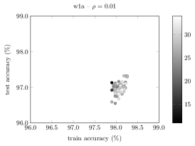
Figure 1: Train vs. test performance for different margins $\rho$ on instance w1a. Each point represents a solution encountered by IPBoost while solving the boosting problem. Grayscale values indicate the number of base learners used in boosted learners; see the legend.

4 Concluding Remarks

In this paper, we have first reproduced the observation that boosting based on column generation, i.e., LP- and IP-boosting, avoids the bad performance on the well-known hard classes from the literature. More importantly, we have shown that IP-boosting improves upon LP-boosting and AdaBoost on the LIBSVM instances on which a consistent improvement even by a few percent is not easy. The price to pay is that the running time with the current implementation is much longer. Nevertheless, the results are promising, so it can make sense to tune the performance, e.g., by solving the intermediate LPs only approximately and deriving tailored heuristics that generate very good primal solutions, see [8] and [7], respectively, for examples for column generation in public transport optimization.

Moreover, our method has a parameter that needs to be tuned, namely the margin bound $\rho$. It shares this property with LP-boosting, where one either needs to set $\rho$ or a corresponding objective weight. AdaBoost, however, depends on the number of iterations which also has to be adjusted to the instance set. We plan to investigate methods based on the approach in the current paper that avoid the dependence on a parameter.

In conclusion, our approach is suited very well to an offline setting in which training may take time and where even a small improvement is beneficial or when convex boosters behave very badly. Moreover, it can serve as a tool to investigate the general performance of such methods.

Appendix A Detailed Computational Results

In the following tables, we report detailed computational results for our tests. We report problem size statistics in Table 3 and running time statistics in Table 4.

For $\rho=0.1,0.075,0.05,0.025,0.01$, we present train results in Tables 5, 7, 9, 13 and test results in Tables 6, 8, 10, 14.

Table 3: Statistics on LIBSVM instances.

	train set				test set
name	$d$	$N$	class $-1$	class $1$	$d$	$N$	class $-1$	class $1$
a1a	$119$	$1605$	$1210$	$395$	–	–	–	–
a2a	$119$	$2265$	$1693$	$572$	–	–	–	–
a3a	$122$	$3185$	$2412$	$773$	–	–	–	–
a4a	$122$	$4781$	$3593$	$1188$	–	–	–	–
a5a	$122$	$6414$	$4845$	$1569$	–	–	–	–
a6a	$122$	$11\,220$	$8528$	$2692$	–	–	–	–
a7a	$122$	$16\,100$	$12\,182$	$3918$	–	–	–	–
a9a	$123$	$32\,561$	$24\,720$	$7841$	–	–	–	–
australian_scale	$14$	$690$	$383$	$307$	–	–	–	–
breast-cancer_scale	$10$	$683$	$444$	$239$	–	–	–	–
cod-rna	$8$	$59\,535$	$39\,690$	$19\,845$	$8$	$271\,617$	$181\,078$	$90\,539$
colon-cancer	$2000$	$62$	$40$	$22$	–	–	–	–
duke	$7129$	$44$	$21$	$23$	$7129$	$38$	$16$	$22$
german.numer	$24$	$1000$	$700$	$300$	–	–	–	–
gisette_scale	$5000$	$6000$	$3000$	$3000$	$5000$	$1000$	$500$	$500$
diabetes_scale	$8$	$768$	$268$	$500$	–	–	–	–
fourclass_scale	$2$	$862$	$555$	$307$	–	–	–	–
german.numer_scale	$24$	$1000$	$700$	$300$	–	–	–	–
heart_scale	$13$	$270$	$150$	$120$	–	–	–	–
ijcnn1	$22$	$49\,990$	$45\,137$	$4853$	$22$	$91\,701$	$82\,989$	$8712$
ionosphere_scale	$34$	$351$	$126$	$225$	–	–	–	–
leu	$7129$	$38$	$11$	$27$	$7129$	$34$	$14$	$20$
liver-disorders	$5$	$145$	$90$	$55$	$5$	$200$	$100$	$100$
madelon	$500$	$2000$	$1000$	$1000$	$500$	$600$	$300$	$300$
phishing	$68$	$11\,055$	$4898$	$6157$	–	–	–	–
skin_nonskin	$3$	$245\,057$	$50\,859$	$194\,198$	–	–	–	–
sonar_scale	$60$	$208$	$111$	$97$	–	–	–	–
splice	$60$	$1000$	$483$	$517$	$60$	$2175$	$1044$	$1131$
svmguide1	$4$	$3089$	$1089$	$2000$	$4$	$4000$	$2000$	$2000$
svmguide3	$22$	$1243$	$947$	$296$	$22$	$41$	$41$	$0$
w1a	$300$	$2477$	$2405$	$72$	$300$	$47\,272$	$45\,865$	$1407$
w2a	$300$	$3470$	$3363$	$107$	$300$	$46\,279$	$44\,907$	$1372$
w3a	$300$	$4912$	$4769$	$143$	$300$	$44\,837$	$43\,501$	$1336$
w4a	$300$	$7366$	$7150$	$216$	$300$	$42\,383$	$41\,120$	$1263$
w5a	$300$	$9888$	$9607$	$281$	$300$	$39\,861$	$38\,663$	$1198$
w8a	$300$	$49\,749$	$48\,270$	$1479$	$300$	$14\,951$	$14\,497$	$454$

Table 4: Statistics for LIBSVM on average run times (in seconds) of different algorithms with $\rho=0.05$ for 10 different seeds; “# optimal” gives the number of instances solved to optimality, “# time out” the number of instances that ran into the time limit of 1 hour, and “best sol. time” the average time at which the best solution was found.

	IPBoost
name	total				best sol.	LPBoost	AdaBoost
name	time	# nodes	# optimal	# time out	time	time	time
a1a	$97.26$	$6669.9$	0	0	$26.08$	$0.15$	$0.40$
a2a	$257.97$	$8186.6$	0	0	$128.55$	$0.26$	$0.59$
a3a	$464.05$	$9096.6$	0	0	$230.18$	$0.37$	$0.59$
a4a	$770.89$	$9769.9$	0	0	$381.76$	$0.73$	$0.83$
a5a	$904.72$	$10\,186.5$	0	0	$465.58$	$1.11$	$1.16$
a6a	$1712.09$	$7763.4$	0	1	$736.32$	$2.76$	$1.76$
a7a	$2946.71$	$8986.1$	0	3	$1542.57$	$5.40$	$2.74$
a8a	$3251.73$	$6370.4$	0	8	$2217.36$	$9.33$	$3.51$
a9a	$3247.98$	$4094.4$	0	7	$1461.27$	$17.96$	$4.89$
australian_scale	$66.84$	$7400.4$	1	0	$23.78$	$0.07$	$0.17$
breast-cancer_scale	$435.32$	$7183.9$	0	1	$29.21$	$0.06$	$0.15$
cod-rna	$3603.83$	$77.4$	0	10	$304.28$	$3281.72$	$30.13$
colon-cancer	$0.09$	$6.8$	10	0	$0.02$	$0.04$	$0.21$
duke	$0.25$	$7.9$	10	0	$0.03$	$0.14$	$0.37$
german.numer	$78.61$	$7215.8$	0	0	$19.77$	$0.09$	$0.20$
gisette_scale	$3439.67$	$3709.8$	0	8	$1991.59$	$18.87$	$16.31$
diabetes_scale	$116.58$	$7313.7$	0	0	$47.29$	$0.07$	$0.17$
fourclass_scale	$165.46$	$9932.6$	0	0	$102.16$	$0.07$	$0.16$
german.numer_scale	$120.73$	$9495.2$	0	0	$62.95$	$0.09$	$0.20$
heart_scale	$43.55$	$10\,170.0$	0	0	$21.58$	$0.03$	$0.14$
ijcnn1	$3604.29$	$1197.2$	0	10	$708.19$	$206.01$	$5.95$
ionosphere_scale	$67.56$	$7375.7$	0	0	$24.33$	$0.08$	$0.16$
leu	$0.20$	$5.8$	10	0	$0.02$	$0.11$	$0.34$
liver-disorders	$48.69$	$9768.9$	0	0	$24.51$	$0.04$	$0.14$
madelon	$2387.03$	$7619.7$	0	5	$1354.16$	$1.59$	$0.90$
mushrooms	$968.38$	$6761.5$	0	0	$248.43$	$2.45$	$1.42$
phishing	$977.76$	$6726.0$	0	0	$268.98$	$3.76$	$1.03$
skin_nonskin	$3576.38$	$2251.6$	0	8	$861.25$	$2967.50$	$9.39$
sonar_scale	$61.81$	$6531.4$	0	0	$19.13$	$0.07$	$0.15$
splice	$128.63$	$5767.6$	0	0	$25.33$	$0.32$	$0.28$
svmguide1	$1375.33$	$9187.1$	0	0	$685.39$	$0.97$	$0.39$
svmguide3	$671.57$	$10\,522.1$	0	0	$400.04$	$0.38$	$0.22$
w1a	$673.90$	$8291.2$	0	0	$240.40$	$3.28$	$6.05$
w2a	$927.73$	$7860.0$	0	0	$353.33$	$3.53$	$6.23$
w3a	$1665.23$	$8071.0$	0	0	$601.93$	$3.80$	$6.30$
w4a	$2442.22$	$8113.1$	0	3	$1256.18$	$3.97$	$6.36$
w5a	$2583.16$	$8091.4$	0	2	$1027.12$	$4.53$	$6.55$
w6a	$3607.69$	$5791.5$	0	10	$1881.83$	$6.17$	$7.42$
w7a	$3607.88$	$4362.3$	0	10	$2106.27$	$7.79$	$7.97$
w8a	$3611.46$	$3204.5$	0	10	$2022.04$	$18.14$	$11.50$
averages	$1367.78$	$6528.4$	$0.8$	$2.4$	$597.53$	$164.35$	$3.59$

Table 5: Averages of the train accuracies and standard deviations for three algorithms with $\rho=0.1$ for 10 different seeds on LIBSVM; best solutions are marked with *; using class probabilities for prediction and voting.

	IPBoost					LPBoost					AdaBoost
name		score			$L$		score			$L$		score			$L$
a1a	*	$79.23$	$\pm$	$1.93$	$4.8$		$77.41$	$\pm$	$1.23$	$4.1$		$77.31$	$\pm$	$1.00$	$9.3$
a2a	*	$78.20$	$\pm$	$1.82$	$4.1$		$77.00$	$\pm$	$1.79$	$5.7$		$76.42$	$\pm$	$0.94$	$9.6$
a3a	*	$77.42$	$\pm$	$1.02$	$4.2$		$76.41$	$\pm$	$0.80$	$4.6$		$77.00$	$\pm$	$1.10$	$10.9$
a4a	*	$77.02$	$\pm$	$1.03$	$4.0$		$75.89$	$\pm$	$0.82$	$4.6$		$76.84$	$\pm$	$1.07$	$11.0$
a5a	*	$77.75$	$\pm$	$0.97$	$4.3$		$76.39$	$\pm$	$0.87$	$4.0$		$77.19$	$\pm$	$0.99$	$11.0$
a6a	*	$77.45$	$\pm$	$0.79$	$3.9$		$76.99$	$\pm$	$1.02$	$4.3$		$77.30$	$\pm$	$1.03$	$11.0$
a7a	*	$77.11$	$\pm$	$1.00$	$3.7$		$76.37$	$\pm$	$1.08$	$3.8$	*	$77.11$	$\pm$	$1.09$	$11.0$
a8a	*	$77.89$	$\pm$	$2.84$	$2.9$		$76.00$	$\pm$	$0.32$	$3.8$		$76.56$	$\pm$	$0.61$	$11.0$
a9a	*	$77.34$	$\pm$	$2.20$	$3.0$		$76.09$	$\pm$	$0.34$	$3.6$		$76.58$	$\pm$	$0.65$	$10.9$
australian_scale	*	$76.56$	$\pm$	$10.27$	$4.4$		$74.55$	$\pm$	$9.16$	$4.7$		$76.03$	$\pm$	$8.71$	$24.1$
breast-cancer_scale	*	$95.89$	$\pm$	$1.46$	$6.2$		$95.32$	$\pm$	$1.50$	$8.4$		$95.27$	$\pm$	$1.65$	$20.2$
cod-rna		$67.89$	$\pm$	$3.82$	$1.3$		$67.87$	$\pm$	$3.80$	$2.4$	*	$68.00$	$\pm$	$4.21$	$55.3$
colon-cancer		$99.00$	$\pm$	$1.41$	$7.6$		$95.20$	$\pm$	$3.01$	$6.4$	*	$100.00$	$\pm$	$0.00$	$58.7$
duke		$99.09$	$\pm$	$1.59$	$6.4$		$95.91$	$\pm$	$2.79$	$4.8$	*	$100.00$	$\pm$	$0.00$	$56.7$
german.numer	*	$71.65$	$\pm$	$1.41$	$4.3$		$70.66$	$\pm$	$1.19$	$3.9$		$71.34$	$\pm$	$1.62$	$19.1$
gisette_scale	*	$82.38$	$\pm$	$4.23$	$4.8$		$79.49$	$\pm$	$6.40$	$9.1$		$82.23$	$\pm$	$3.26$	$95.1$
diabetes_scale		$69.20$	$\pm$	$4.23$	$4.2$		$69.28$	$\pm$	$3.85$	$4.9$	*	$73.54$	$\pm$	$3.60$	$46.2$
fourclass_scale		$73.16$	$\pm$	$1.93$	$3.1$		$73.65$	$\pm$	$1.79$	$4.2$	*	$76.41$	$\pm$	$1.40$	$38.0$
german.numer_scale	*	$71.66$	$\pm$	$1.43$	$4.6$		$70.66$	$\pm$	$1.19$	$3.9$		$71.34$	$\pm$	$1.62$	$19.1$
heart_scale	*	$77.27$	$\pm$	$3.83$	$4.3$		$75.05$	$\pm$	$3.57$	$4.6$		$77.13$	$\pm$	$5.64$	$20.1$
ijcnn1		$90.31$	$\pm$	$0.08$	$3.5$	*	$90.45$	$\pm$	$0.46$	$5.3$		$90.34$	$\pm$	$0.06$	$71.6$
ionosphere_scale		$90.00$	$\pm$	$2.89$	$6.4$		$89.61$	$\pm$	$2.89$	$10.3$	*	$97.62$	$\pm$	$2.07$	$49.1$
leu		$98.42$	$\pm$	$1.84$	$3.4$		$92.37$	$\pm$	$3.15$	$2.7$	*	$100.00$	$\pm$	$0.00$	$36.9$
liver-disorders		$77.17$	$\pm$	$1.76$	$5.4$		$75.93$	$\pm$	$2.61$	$6.2$	*	$84.83$	$\pm$	$1.81$	$37.5$
madelon		$55.80$	$\pm$	$2.57$	$6.0$		$55.08$	$\pm$	$2.85$	$3.1$	*	$67.29$	$\pm$	$1.79$	$97.2$
mushrooms	*	$86.78$	$\pm$	$9.01$	$5.2$		$78.89$	$\pm$	$10.42$	$6.1$		$77.60$	$\pm$	$6.31$	$9.7$
phishing	*	$79.39$	$\pm$	$10.55$	$2.5$		$76.63$	$\pm$	$12.79$	$3.9$		$71.67$	$\pm$	$8.51$	$8.0$
skin_nonskin		$83.04$	$\pm$	$4.50$	$2.4$		$82.88$	$\pm$	$4.69$	$3.1$	*	$83.33$	$\pm$	$4.64$	$50.4$
sonar_scale		$79.34$	$\pm$	$4.62$	$5.1$		$80.36$	$\pm$	$4.25$	$13.0$	*	$99.46$	$\pm$	$0.82$	$64.6$
splice		$65.68$	$\pm$	$7.26$	$3.7$		$64.68$	$\pm$	$7.70$	$6.5$	*	$66.89$	$\pm$	$6.23$	$21.0$
svmguide1		$92.61$	$\pm$	$3.80$	$5.5$		$92.28$	$\pm$	$4.00$	$6.5$	*	$92.92$	$\pm$	$3.71$	$62.9$
svmguide3		$78.87$	$\pm$	$1.46$	$4.8$		$78.21$	$\pm$	$1.32$	$6.0$	*	$81.36$	$\pm$	$2.38$	$70.7$
w1a	*	$97.76$	$\pm$	$0.14$	$6.6$		$97.47$	$\pm$	$0.18$	$5.3$		$97.31$	$\pm$	$0.15$	$14.9$
w2a	*	$97.54$	$\pm$	$0.14$	$6.1$		$97.22$	$\pm$	$0.16$	$4.8$		$97.13$	$\pm$	$0.10$	$15.5$
w3a	*	$97.56$	$\pm$	$0.17$	$6.1$		$97.31$	$\pm$	$0.10$	$5.3$		$97.25$	$\pm$	$0.12$	$16.1$
w4a	*	$97.52$	$\pm$	$0.12$	$6.0$		$97.28$	$\pm$	$0.08$	$5.5$		$97.21$	$\pm$	$0.10$	$16.1$
w5a	*	$97.56$	$\pm$	$0.07$	$6.3$		$97.29$	$\pm$	$0.05$	$4.6$		$97.28$	$\pm$	$0.10$	$16.1$
w6a	*	$97.32$	$\pm$	$0.13$	$5.9$		$97.16$	$\pm$	$0.11$	$5.7$		$97.11$	$\pm$	$0.13$	$16.1$
w7a	*	$97.38$	$\pm$	$0.12$	$5.9$		$97.18$	$\pm$	$0.11$	$5.5$		$97.16$	$\pm$	$0.11$	$16.1$
w8a	*	$97.40$	$\pm$	$0.12$	$5.8$		$97.21$	$\pm$	$0.10$	$5.6$		$97.19$	$\pm$	$0.11$	$16.5$
averages	$25$	$83.52$	$\pm$	$2.51$	$4.7$	$1$	$82.29$	$\pm$	$2.61$	$5.3$	$15$	$84.36$	$\pm$	$1.99$	$31.4$

Table 6: Averages of the test accuracies and standard deviations for three algorithms with $\rho=0.1$ for 10 different seeds on LIBSVM; best solutions are marked with *; using class probabilities for prediction and voting.

	IPBoost					LPBoost					AdaBoost
name		score			$L$		score			$L$		score			$L$
a1a	*	$78.32$	$\pm$	$3.25$	$4.8$		$76.70$	$\pm$	$2.94$	$4.1$		$76.04$	$\pm$	$3.30$	$9.3$
a2a	*	$77.88$	$\pm$	$2.23$	$4.1$		$76.51$	$\pm$	$2.30$	$5.7$		$75.67$	$\pm$	$1.57$	$9.6$
a3a	*	$77.47$	$\pm$	$1.39$	$4.2$		$75.64$	$\pm$	$1.62$	$4.6$		$76.84$	$\pm$	$1.03$	$10.9$
a4a	*	$76.44$	$\pm$	$1.93$	$4.0$		$75.23$	$\pm$	$1.75$	$4.6$		$76.18$	$\pm$	$1.72$	$11.0$
a5a	*	$77.18$	$\pm$	$1.51$	$4.3$		$75.70$	$\pm$	$1.85$	$4.0$		$76.72$	$\pm$	$1.77$	$11.0$
a6a		$77.77$	$\pm$	$1.22$	$3.9$		$77.58$	$\pm$	$1.35$	$4.3$	*	$77.84$	$\pm$	$1.31$	$11.0$
a7a		$77.23$	$\pm$	$1.26$	$3.7$		$76.52$	$\pm$	$1.10$	$3.8$	*	$77.28$	$\pm$	$1.39$	$11.0$
a8a	*	$77.96$	$\pm$	$2.69$	$2.9$		$75.97$	$\pm$	$0.49$	$3.8$		$76.46$	$\pm$	$0.64$	$11.0$
a9a	*	$77.35$	$\pm$	$2.29$	$3.0$		$76.24$	$\pm$	$0.58$	$3.6$		$76.54$	$\pm$	$0.82$	$10.9$
australian_scale	*	$75.00$	$\pm$	$10.15$	$4.4$		$72.32$	$\pm$	$9.84$	$4.7$		$72.61$	$\pm$	$9.54$	$24.1$
breast-cancer_scale	*	$93.97$	$\pm$	$1.89$	$6.2$		$93.09$	$\pm$	$2.53$	$8.4$		$93.01$	$\pm$	$2.48$	$20.2$
cod-rna		$67.82$	$\pm$	$3.66$	$1.3$		$67.78$	$\pm$	$3.51$	$2.4$	*	$67.94$	$\pm$	$4.03$	$55.3$
colon-cancer		$71.67$	$\pm$	$13.15$	$7.6$		$70.83$	$\pm$	$9.82$	$6.4$	*	$76.67$	$\pm$	$14.59$	$58.7$
duke		$98.95$	$\pm$	$1.84$	$6.4$		$95.53$	$\pm$	$3.05$	$4.8$	*	$100.00$	$\pm$	$0.00$	$56.7$
german.numer	*	$72.35$	$\pm$	$3.64$	$4.3$		$71.90$	$\pm$	$3.26$	$3.9$		$71.80$	$\pm$	$3.32$	$19.1$
gisette_scale	*	$81.40$	$\pm$	$4.69$	$4.8$		$79.05$	$\pm$	$5.96$	$9.1$		$80.40$	$\pm$	$3.62$	$95.1$
diabetes_scale		$67.32$	$\pm$	$6.22$	$4.2$	*	$68.04$	$\pm$	$4.97$	$4.9$		$66.80$	$\pm$	$5.07$	$46.2$
fourclass_scale		$72.33$	$\pm$	$5.19$	$3.1$	*	$72.44$	$\pm$	$4.29$	$4.2$		$72.09$	$\pm$	$4.02$	$38.0$
german.numer_scale	*	$72.25$	$\pm$	$3.63$	$4.6$		$71.90$	$\pm$	$3.26$	$3.9$		$71.80$	$\pm$	$3.32$	$19.1$
heart_scale	*	$73.70$	$\pm$	$6.52$	$4.3$		$71.30$	$\pm$	$4.80$	$4.6$		$69.81$	$\pm$	$5.09$	$20.1$
ijcnn1		$90.34$	$\pm$	$0.22$	$3.5$	*	$90.63$	$\pm$	$0.89$	$5.3$		$90.30$	$\pm$	$0.28$	$71.6$
ionosphere_scale		$84.71$	$\pm$	$5.43$	$6.4$		$85.57$	$\pm$	$4.18$	$10.3$	*	$86.71$	$\pm$	$4.86$	$49.1$
leu		$70.29$	$\pm$	$7.26$	$3.4$		$73.24$	$\pm$	$8.48$	$2.7$	*	$80.88$	$\pm$	$7.50$	$36.9$
liver-disorders		$54.35$	$\pm$	$2.70$	$5.4$	*	$55.95$	$\pm$	$3.20$	$6.2$		$55.90$	$\pm$	$3.02$	$37.5$
madelon		$53.30$	$\pm$	$4.44$	$6.0$	*	$53.67$	$\pm$	$4.22$	$3.1$		$52.12$	$\pm$	$1.82$	$97.2$
mushrooms	*	$87.08$	$\pm$	$8.65$	$5.2$		$79.35$	$\pm$	$10.05$	$6.1$		$77.70$	$\pm$	$6.29$	$9.7$
phishing	*	$79.02$	$\pm$	$10.87$	$2.5$		$76.63$	$\pm$	$12.76$	$3.9$		$71.27$	$\pm$	$8.52$	$8.0$
skin_nonskin		$83.06$	$\pm$	$4.56$	$2.4$		$82.91$	$\pm$	$4.76$	$3.1$	*	$83.35$	$\pm$	$4.71$	$50.4$
sonar_scale		$66.83$	$\pm$	$8.54$	$5.1$	*	$69.27$	$\pm$	$9.14$	$13.0$		$63.90$	$\pm$	$11.14$	$64.6$
splice		$65.14$	$\pm$	$7.83$	$3.7$		$64.67$	$\pm$	$8.02$	$6.5$	*	$65.19$	$\pm$	$6.65$	$21.0$
svmguide1	*	$90.77$	$\pm$	$4.88$	$5.5$		$90.69$	$\pm$	$4.78$	$6.5$		$90.40$	$\pm$	$5.01$	$62.9$
svmguide3		$79.76$	$\pm$	$18.54$	$4.8$	*	$86.10$	$\pm$	$16.78$	$6.0$		$63.90$	$\pm$	$23.36$	$70.7$
w1a	*	$97.29$	$\pm$	$0.17$	$6.6$		$97.21$	$\pm$	$0.12$	$5.3$		$97.11$	$\pm$	$0.14$	$14.9$
w2a	*	$97.38$	$\pm$	$0.13$	$6.1$		$97.21$	$\pm$	$0.09$	$4.8$		$97.15$	$\pm$	$0.11$	$15.5$
w3a	*	$97.35$	$\pm$	$0.11$	$6.1$		$97.21$	$\pm$	$0.10$	$5.3$		$97.18$	$\pm$	$0.11$	$16.1$
w4a	*	$97.37$	$\pm$	$0.16$	$6.0$		$97.18$	$\pm$	$0.10$	$5.5$		$97.17$	$\pm$	$0.12$	$16.1$
w5a	*	$97.37$	$\pm$	$0.11$	$6.3$		$97.13$	$\pm$	$0.08$	$4.6$		$97.14$	$\pm$	$0.11$	$16.1$
w6a	*	$97.38$	$\pm$	$0.13$	$5.9$		$97.23$	$\pm$	$0.09$	$5.7$		$97.22$	$\pm$	$0.11$	$16.1$
w7a	*	$97.39$	$\pm$	$0.12$	$5.9$		$97.21$	$\pm$	$0.10$	$5.5$		$97.21$	$\pm$	$0.11$	$16.1$
w8a	*	$97.26$	$\pm$	$0.12$	$5.8$		$97.13$	$\pm$	$0.10$	$5.6$		$97.12$	$\pm$	$0.10$	$16.5$
averages	$24$	$80.70$	$\pm$	$4.08$	$4.7$	$7$	$80.16$	$\pm$	$3.93$	$5.3$	$9$	$79.79$	$\pm$	$3.82$	$31.4$

Table 7: Averages of the train accuracies and standard deviations for three algorithms with $\rho=0.075$ for 10 different seeds on LIBSVM; best solutions are marked with *; using class probabilities for prediction and voting.

	IPBoost					LPBoost					AdaBoost
name		score			$L$		score			$L$		score			$L$
a1a	*	$79.35$	$\pm$	$2.14$	$5.5$		$77.37$	$\pm$	$1.20$	$4.7$		$77.31$	$\pm$	$1.00$	$9.3$
a2a	*	$78.68$	$\pm$	$1.60$	$5.4$		$77.25$	$\pm$	$1.88$	$6.3$		$76.42$	$\pm$	$0.94$	$9.6$
a3a	*	$78.05$	$\pm$	$1.11$	$6.0$		$76.43$	$\pm$	$0.82$	$5.0$		$77.00$	$\pm$	$1.10$	$10.9$
a4a	*	$77.73$	$\pm$	$0.95$	$6.0$		$75.90$	$\pm$	$0.82$	$4.5$		$76.84$	$\pm$	$1.07$	$11.0$
a5a	*	$78.18$	$\pm$	$1.28$	$5.3$		$76.40$	$\pm$	$0.87$	$4.4$		$77.19$	$\pm$	$0.99$	$11.0$
a6a	*	$77.68$	$\pm$	$0.99$	$4.6$		$76.73$	$\pm$	$0.95$	$3.9$		$77.30$	$\pm$	$1.03$	$11.0$
a7a	*	$77.45$	$\pm$	$1.22$	$5.4$		$76.37$	$\pm$	$1.08$	$3.7$		$77.11$	$\pm$	$1.09$	$11.0$
a8a	*	$77.84$	$\pm$	$2.45$	$3.6$		$76.01$	$\pm$	$0.32$	$3.8$		$76.56$	$\pm$	$0.61$	$11.0$
a9a	*	$76.87$	$\pm$	$1.76$	$3.0$		$76.09$	$\pm$	$0.34$	$3.6$		$76.58$	$\pm$	$0.65$	$10.9$
australian_scale		$76.00$	$\pm$	$9.33$	$5.6$		$74.66$	$\pm$	$9.10$	$4.9$	*	$76.03$	$\pm$	$8.71$	$24.1$
breast-cancer_scale	*	$96.36$	$\pm$	$1.01$	$7.5$		$95.36$	$\pm$	$1.51$	$9.7$		$95.27$	$\pm$	$1.65$	$20.2$
cod-rna		$67.89$	$\pm$	$3.82$	$1.5$		$67.87$	$\pm$	$3.80$	$2.4$	*	$68.00$	$\pm$	$4.21$	$55.3$
colon-cancer		$98.80$	$\pm$	$1.40$	$6.3$		$94.40$	$\pm$	$1.58$	$5.1$	*	$100.00$	$\pm$	$0.00$	$58.7$
duke		$98.41$	$\pm$	$1.87$	$5.9$		$96.14$	$\pm$	$2.84$	$5.0$	*	$100.00$	$\pm$	$0.00$	$56.7$
german.numer	*	$71.84$	$\pm$	$1.64$	$5.1$		$70.67$	$\pm$	$1.19$	$4.2$		$71.34$	$\pm$	$1.62$	$19.1$
gisette_scale	*	$83.14$	$\pm$	$3.31$	$5.5$		$81.94$	$\pm$	$4.56$	$13.5$		$82.23$	$\pm$	$3.26$	$95.1$
diabetes_scale		$69.98$	$\pm$	$4.30$	$5.7$		$69.67$	$\pm$	$4.12$	$5.3$	*	$73.54$	$\pm$	$3.60$	$46.2$
fourclass_scale		$74.13$	$\pm$	$1.81$	$4.0$		$74.26$	$\pm$	$1.43$	$5.5$	*	$76.41$	$\pm$	$1.40$	$38.0$
german.numer_scale	*	$71.73$	$\pm$	$1.51$	$5.5$		$70.67$	$\pm$	$1.19$	$4.2$		$71.34$	$\pm$	$1.62$	$19.1$
heart_scale	*	$78.84$	$\pm$	$3.54$	$6.3$		$75.42$	$\pm$	$3.80$	$5.3$		$77.13$	$\pm$	$5.64$	$20.1$
ijcnn1		$90.42$	$\pm$	$0.23$	$4.4$	*	$90.45$	$\pm$	$0.46$	$6.1$		$90.34$	$\pm$	$0.06$	$71.6$
ionosphere_scale		$91.28$	$\pm$	$2.72$	$7.1$		$91.00$	$\pm$	$2.98$	$13.9$	*	$97.62$	$\pm$	$2.07$	$49.1$
leu		$98.68$	$\pm$	$1.86$	$3.4$		$92.37$	$\pm$	$3.15$	$2.7$	*	$100.00$	$\pm$	$0.00$	$36.9$
liver-disorders		$78.14$	$\pm$	$2.03$	$6.7$		$76.07$	$\pm$	$2.43$	$7.4$	*	$84.83$	$\pm$	$1.81$	$37.5$
madelon		$56.13$	$\pm$	$2.84$	$9.9$		$55.47$	$\pm$	$2.88$	$3.6$	*	$67.29$	$\pm$	$1.79$	$97.2$
mushrooms	*	$88.14$	$\pm$	$7.75$	$6.0$		$79.50$	$\pm$	$10.21$	$6.0$		$77.60$	$\pm$	$6.31$	$9.7$
phishing	*	$83.89$	$\pm$	$7.85$	$3.5$		$76.54$	$\pm$	$12.87$	$4.1$		$71.67$	$\pm$	$8.51$	$8.0$
skin_nonskin		$83.04$	$\pm$	$4.54$	$2.0$		$82.91$	$\pm$	$4.73$	$3.6$	*	$83.33$	$\pm$	$4.64$	$50.4$
sonar_scale		$80.30$	$\pm$	$4.68$	$6.1$		$83.11$	$\pm$	$4.81$	$17.6$	*	$99.46$	$\pm$	$0.82$	$64.6$
splice		$65.83$	$\pm$	$7.11$	$4.8$		$64.76$	$\pm$	$7.64$	$7.2$	*	$66.89$	$\pm$	$6.23$	$21.0$
svmguide1		$92.73$	$\pm$	$3.73$	$6.3$		$92.34$	$\pm$	$3.90$	$6.8$	*	$92.92$	$\pm$	$3.71$	$62.9$
svmguide3		$79.40$	$\pm$	$1.59$	$6.4$		$78.54$	$\pm$	$1.24$	$7.0$	*	$81.36$	$\pm$	$2.38$	$70.7$
w1a	*	$97.88$	$\pm$	$0.15$	$7.9$		$97.46$	$\pm$	$0.20$	$5.6$		$97.31$	$\pm$	$0.15$	$14.9$
w2a	*	$97.67$	$\pm$	$0.21$	$8.5$		$97.23$	$\pm$	$0.18$	$5.0$		$97.13$	$\pm$	$0.10$	$15.5$
w3a	*	$97.65$	$\pm$	$0.16$	$7.9$		$97.31$	$\pm$	$0.11$	$6.0$		$97.25$	$\pm$	$0.12$	$16.1$
w4a	*	$97.59$	$\pm$	$0.10$	$8.4$		$97.28$	$\pm$	$0.09$	$5.8$		$97.21$	$\pm$	$0.10$	$16.1$
w5a	*	$97.61$	$\pm$	$0.12$	$7.6$		$97.30$	$\pm$	$0.05$	$4.8$		$97.28$	$\pm$	$0.10$	$16.1$
w6a	*	$97.45$	$\pm$	$0.15$	$7.9$		$97.16$	$\pm$	$0.11$	$5.8$		$97.11$	$\pm$	$0.13$	$16.1$
w7a	*	$97.43$	$\pm$	$0.11$	$7.2$		$97.19$	$\pm$	$0.11$	$5.6$		$97.16$	$\pm$	$0.11$	$16.1$
w8a	*	$97.42$	$\pm$	$0.12$	$7.2$		$97.21$	$\pm$	$0.10$	$5.7$		$97.19$	$\pm$	$0.11$	$16.5$
averages	$24$	$83.94$	$\pm$	$2.38$	$5.8$	$1$	$82.52$	$\pm$	$2.54$	$5.9$	$15$	$84.36$	$\pm$	$1.99$	$31.4$

Table 8: Averages of the test accuracies and standard deviations for three algorithms with $\rho=0.075$ for 10 different seeds on LIBSVM; best solutions are marked with *; using class probabilities for prediction and voting.

	IPBoost					LPBoost					AdaBoost
name		score			$L$		score			$L$		score			$L$
a1a	*	$78.60$	$\pm$	$3.49$	$5.5$		$76.73$	$\pm$	$2.94$	$4.7$		$76.04$	$\pm$	$3.30$	$9.3$
a2a	*	$78.28$	$\pm$	$1.69$	$5.4$		$76.62$	$\pm$	$2.35$	$6.3$		$75.67$	$\pm$	$1.57$	$9.6$
a3a	*	$77.60$	$\pm$	$1.19$	$6.0$		$75.60$	$\pm$	$1.60$	$5.0$		$76.84$	$\pm$	$1.03$	$10.9$
a4a	*	$76.90$	$\pm$	$2.10$	$6.0$		$75.23$	$\pm$	$1.75$	$4.5$		$76.18$	$\pm$	$1.72$	$11.0$
a5a	*	$77.46$	$\pm$	$1.71$	$5.3$		$75.73$	$\pm$	$1.87$	$4.4$		$76.72$	$\pm$	$1.77$	$11.0$
a6a	*	$78.08$	$\pm$	$1.23$	$4.6$		$77.42$	$\pm$	$1.05$	$3.9$		$77.84$	$\pm$	$1.31$	$11.0$
a7a	*	$77.52$	$\pm$	$1.33$	$5.4$		$76.52$	$\pm$	$1.10$	$3.7$		$77.28$	$\pm$	$1.39$	$11.0$
a8a	*	$77.84$	$\pm$	$2.40$	$3.6$		$75.97$	$\pm$	$0.49$	$3.8$		$76.46$	$\pm$	$0.64$	$11.0$
a9a	*	$76.91$	$\pm$	$2.09$	$3.0$		$76.24$	$\pm$	$0.58$	$3.6$		$76.54$	$\pm$	$0.82$	$10.9$
australian_scale		$72.46$	$\pm$	$9.38$	$5.6$		$72.54$	$\pm$	$9.86$	$4.9$	*	$72.61$	$\pm$	$9.54$	$24.1$
breast-cancer_scale	*	$93.46$	$\pm$	$2.18$	$7.5$		$93.24$	$\pm$	$2.13$	$9.7$		$93.01$	$\pm$	$2.48$	$20.2$
cod-rna		$67.82$	$\pm$	$3.66$	$1.5$		$67.77$	$\pm$	$3.50$	$2.4$	*	$67.94$	$\pm$	$4.03$	$55.3$
colon-cancer		$70.83$	$\pm$	$9.82$	$6.3$		$71.67$	$\pm$	$10.54$	$5.1$	*	$76.67$	$\pm$	$14.59$	$58.7$
duke		$98.16$	$\pm$	$2.17$	$5.9$		$95.79$	$\pm$	$3.09$	$5.0$	*	$100.00$	$\pm$	$0.00$	$56.7$
german.numer	*	$72.50$	$\pm$	$3.44$	$5.1$		$71.85$	$\pm$	$3.22$	$4.2$		$71.80$	$\pm$	$3.32$	$19.1$
gisette_scale	*	$82.38$	$\pm$	$4.17$	$5.5$		$81.28$	$\pm$	$4.22$	$13.5$		$80.40$	$\pm$	$3.62$	$95.1$
diabetes_scale		$66.80$	$\pm$	$5.09$	$5.7$	*	$67.58$	$\pm$	$4.02$	$5.3$		$66.80$	$\pm$	$5.07$	$46.2$
fourclass_scale		$72.50$	$\pm$	$4.64$	$4.0$	*	$73.08$	$\pm$	$3.80$	$5.5$		$72.09$	$\pm$	$4.02$	$38.0$
german.numer_scale	*	$72.10$	$\pm$	$3.21$	$5.5$		$71.85$	$\pm$	$3.22$	$4.2$		$71.80$	$\pm$	$3.32$	$19.1$
heart_scale	*	$71.48$	$\pm$	$6.88$	$6.3$		$71.11$	$\pm$	$4.55$	$5.3$		$69.81$	$\pm$	$5.09$	$20.1$
ijcnn1		$90.42$	$\pm$	$0.34$	$4.4$	*	$90.60$	$\pm$	$0.90$	$6.1$		$90.30$	$\pm$	$0.28$	$71.6$
ionosphere_scale		$86.14$	$\pm$	$5.68$	$7.1$		$86.14$	$\pm$	$5.47$	$13.9$	*	$86.71$	$\pm$	$4.86$	$49.1$
leu		$71.18$	$\pm$	$7.57$	$3.4$		$73.24$	$\pm$	$8.48$	$2.7$	*	$80.88$	$\pm$	$7.50$	$36.9$
liver-disorders		$54.90$	$\pm$	$3.16$	$6.7$		$55.85$	$\pm$	$3.11$	$7.4$	*	$55.90$	$\pm$	$3.02$	$37.5$
madelon		$52.88$	$\pm$	$4.27$	$9.9$	*	$53.45$	$\pm$	$4.24$	$3.6$		$52.12$	$\pm$	$1.82$	$97.2$
mushrooms	*	$88.17$	$\pm$	$8.18$	$6.0$		$79.76$	$\pm$	$9.96$	$6.0$		$77.70$	$\pm$	$6.29$	$9.7$
phishing	*	$83.72$	$\pm$	$8.15$	$3.5$		$76.46$	$\pm$	$12.91$	$4.1$		$71.27$	$\pm$	$8.52$	$8.0$
skin_nonskin		$83.03$	$\pm$	$4.61$	$2.0$		$82.94$	$\pm$	$4.79$	$3.6$	*	$83.35$	$\pm$	$4.71$	$50.4$
sonar_scale		$67.32$	$\pm$	$9.97$	$6.1$	*	$69.76$	$\pm$	$8.70$	$17.6$		$63.90$	$\pm$	$11.14$	$64.6$
splice		$65.03$	$\pm$	$7.84$	$4.8$		$64.69$	$\pm$	$8.00$	$7.2$	*	$65.19$	$\pm$	$6.65$	$21.0$
svmguide1	*	$90.93$	$\pm$	$4.72$	$6.3$		$90.92$	$\pm$	$4.48$	$6.8$		$90.40$	$\pm$	$5.01$	$62.9$
svmguide3		$78.29$	$\pm$	$18.09$	$6.4$	*	$83.17$	$\pm$	$17.83$	$7.0$		$63.90$	$\pm$	$23.36$	$70.7$
w1a	*	$97.31$	$\pm$	$0.22$	$7.9$		$97.19$	$\pm$	$0.11$	$5.6$		$97.11$	$\pm$	$0.14$	$14.9$
w2a	*	$97.45$	$\pm$	$0.14$	$8.5$		$97.21$	$\pm$	$0.09$	$5.0$		$97.15$	$\pm$	$0.11$	$15.5$
w3a	*	$97.40$	$\pm$	$0.14$	$7.9$		$97.20$	$\pm$	$0.11$	$6.0$		$97.18$	$\pm$	$0.11$	$16.1$
w4a	*	$97.46$	$\pm$	$0.11$	$8.4$		$97.20$	$\pm$	$0.10$	$5.8$		$97.17$	$\pm$	$0.12$	$16.1$
w5a	*	$97.42$	$\pm$	$0.14$	$7.6$		$97.14$	$\pm$	$0.08$	$4.8$		$97.14$	$\pm$	$0.11$	$16.1$
w6a	*	$97.47$	$\pm$	$0.14$	$7.9$		$97.23$	$\pm$	$0.09$	$5.8$		$97.22$	$\pm$	$0.11$	$16.1$
w7a	*	$97.42$	$\pm$	$0.08$	$7.2$		$97.21$	$\pm$	$0.11$	$5.6$		$97.21$	$\pm$	$0.11$	$16.1$
w8a	*	$97.27$	$\pm$	$0.13$	$7.2$		$97.13$	$\pm$	$0.11$	$5.7$		$97.12$	$\pm$	$0.10$	$16.5$
averages	$25$	$80.77$	$\pm$	$3.89$	$5.8$	$6$	$80.21$	$\pm$	$3.89$	$5.9$	$9$	$79.79$	$\pm$	$3.82$	$31.4$

Table 9: Averages of the train accuracies and standard deviations for three algorithms with $\rho=0.05$ for 10 different seeds on LIBSVM; best solutions are marked with *; using class probabilities for prediction and voting.

	IPBoost					LPBoost					AdaBoost
name		score			$L$		score			$L$		score			$L$
a1a	*	$79.97$	$\pm$	$1.80$	$7.0$		$77.41$	$\pm$	$1.23$	$4.6$		$77.31$	$\pm$	$1.00$	$9.3$
a2a	*	$79.06$	$\pm$	$1.73$	$6.2$		$76.66$	$\pm$	$1.01$	$6.5$		$76.42$	$\pm$	$0.94$	$9.6$
a3a	*	$78.67$	$\pm$	$1.08$	$7.9$		$76.37$	$\pm$	$0.83$	$5.0$		$77.00$	$\pm$	$1.10$	$10.9$
a4a	*	$78.24$	$\pm$	$1.27$	$7.8$		$75.93$	$\pm$	$0.82$	$4.8$		$76.84$	$\pm$	$1.07$	$11.0$
a5a	*	$78.46$	$\pm$	$1.18$	$7.8$		$76.41$	$\pm$	$0.87$	$4.4$		$77.19$	$\pm$	$0.99$	$11.0$
a6a	*	$77.94$	$\pm$	$0.84$	$6.7$		$76.94$	$\pm$	$0.96$	$4.9$		$77.30$	$\pm$	$1.03$	$11.0$
a7a	*	$77.69$	$\pm$	$1.05$	$7.1$		$76.37$	$\pm$	$1.09$	$4.2$		$77.11$	$\pm$	$1.09$	$11.0$
a8a	*	$78.11$	$\pm$	$2.44$	$4.5$		$76.01$	$\pm$	$0.32$	$4.1$		$76.56$	$\pm$	$0.61$	$11.0$
a9a		$76.31$	$\pm$	$0.58$	$2.9$		$76.09$	$\pm$	$0.34$	$3.7$	*	$76.58$	$\pm$	$0.65$	$10.9$
australian_scale	*	$77.52$	$\pm$	$9.86$	$7.3$		$74.86$	$\pm$	$8.97$	$5.8$		$76.03$	$\pm$	$8.71$	$24.1$
breast-cancer_scale	*	$96.49$	$\pm$	$1.43$	$9.6$		$95.63$	$\pm$	$1.56$	$9.8$		$95.27$	$\pm$	$1.65$	$20.2$
cod-rna	*	$68.10$	$\pm$	$4.49$	$1.8$		$67.90$	$\pm$	$3.91$	$2.4$		$68.00$	$\pm$	$4.21$	$55.3$
colon-cancer		$98.20$	$\pm$	$1.48$	$5.5$		$94.20$	$\pm$	$1.48$	$5.1$	*	$100.00$	$\pm$	$0.00$	$58.7$
duke		$97.73$	$\pm$	$1.86$	$5.6$		$96.14$	$\pm$	$2.84$	$5.0$	*	$100.00$	$\pm$	$0.00$	$56.7$
german.numer	*	$71.90$	$\pm$	$1.92$	$6.5$		$70.67$	$\pm$	$1.19$	$4.4$		$71.34$	$\pm$	$1.62$	$19.1$
gisette_scale	*	$84.60$	$\pm$	$2.93$	$7.0$		$83.90$	$\pm$	$3.73$	$20.9$		$82.23$	$\pm$	$3.26$	$95.1$
diabetes_scale		$71.07$	$\pm$	$3.75$	$7.4$		$69.93$	$\pm$	$3.89$	$6.6$	*	$73.54$	$\pm$	$3.60$	$46.2$
fourclass_scale		$76.29$	$\pm$	$1.56$	$8.6$		$74.33$	$\pm$	$1.58$	$6.1$	*	$76.41$	$\pm$	$1.40$	$38.0$
german.numer_scale	*	$72.01$	$\pm$	$1.98$	$6.5$		$70.68$	$\pm$	$1.19$	$4.4$		$71.34$	$\pm$	$1.62$	$19.1$
heart_scale	*	$81.02$	$\pm$	$2.90$	$7.3$		$75.79$	$\pm$	$4.08$	$6.4$		$77.13$	$\pm$	$5.64$	$20.1$
ijcnn1	*	$90.47$	$\pm$	$0.47$	$5.8$	*	$90.47$	$\pm$	$0.45$	$7.9$		$90.34$	$\pm$	$0.06$	$71.6$
ionosphere_scale		$92.56$	$\pm$	$2.59$	$9.2$		$92.21$	$\pm$	$3.06$	$19.5$	*	$97.62$	$\pm$	$2.07$	$49.1$
leu		$98.68$	$\pm$	$1.86$	$3.5$		$92.37$	$\pm$	$3.15$	$2.7$	*	$100.00$	$\pm$	$0.00$	$36.9$
liver-disorders		$80.28$	$\pm$	$2.16$	$9.1$		$77.38$	$\pm$	$2.00$	$9.5$	*	$84.83$	$\pm$	$1.81$	$37.5$
madelon		$56.45$	$\pm$	$3.08$	$31.4$		$56.69$	$\pm$	$2.67$	$14.0$	*	$67.28$	$\pm$	$1.79$	$97.2$
mushrooms	*	$87.86$	$\pm$	$7.83$	$8.6$		$81.60$	$\pm$	$8.18$	$7.0$		$77.60$	$\pm$	$6.31$	$9.7$
phishing	*	$80.86$	$\pm$	$10.96$	$3.5$		$76.96$	$\pm$	$12.46$	$4.0$		$71.67$	$\pm$	$8.51$	$8.0$
skin_nonskin		$83.12$	$\pm$	$4.60$	$2.5$		$82.91$	$\pm$	$4.73$	$3.7$	*	$83.33$	$\pm$	$4.64$	$50.4$
sonar_scale		$83.53$	$\pm$	$3.76$	$12.3$		$88.08$	$\pm$	$4.43$	$25.4$	*	$99.46$	$\pm$	$0.82$	$64.6$
splice		$66.25$	$\pm$	$6.92$	$5.0$		$65.74$	$\pm$	$6.97$	$7.6$	*	$66.89$	$\pm$	$6.23$	$21.0$
svmguide1		$92.90$	$\pm$	$3.78$	$8.6$		$92.53$	$\pm$	$3.84$	$6.9$	*	$92.92$	$\pm$	$3.71$	$62.9$
svmguide3		$79.69$	$\pm$	$1.79$	$8.6$		$78.65$	$\pm$	$1.35$	$8.9$	*	$81.36$	$\pm$	$2.38$	$70.7$
w1a	*	$98.07$	$\pm$	$0.19$	$10.8$		$97.46$	$\pm$	$0.18$	$5.2$		$97.31$	$\pm$	$0.15$	$14.9$
w2a	*	$97.78$	$\pm$	$0.22$	$10.7$		$97.25$	$\pm$	$0.17$	$5.5$		$97.13$	$\pm$	$0.10$	$15.5$
w3a	*	$97.75$	$\pm$	$0.16$	$11.0$		$97.33$	$\pm$	$0.15$	$6.6$		$97.25$	$\pm$	$0.12$	$16.1$
w4a	*	$97.67$	$\pm$	$0.13$	$10.9$		$97.31$	$\pm$	$0.10$	$6.0$		$97.21$	$\pm$	$0.10$	$16.1$
w5a	*	$97.68$	$\pm$	$0.13$	$11.1$		$97.32$	$\pm$	$0.08$	$5.0$		$97.28$	$\pm$	$0.10$	$16.1$
w6a	*	$97.49$	$\pm$	$0.16$	$10.2$		$97.17$	$\pm$	$0.11$	$5.7$		$97.11$	$\pm$	$0.13$	$16.1$
w7a	*	$97.48$	$\pm$	$0.12$	$10.1$		$97.19$	$\pm$	$0.12$	$5.6$		$97.16$	$\pm$	$0.11$	$16.1$
w8a	*	$97.52$	$\pm$	$0.11$	$9.8$		$97.20$	$\pm$	$0.10$	$5.6$		$97.19$	$\pm$	$0.11$	$16.5$
averages	$26$	$84.34$	$\pm$	$2.43$	$8.1$	$1$	$82.90$	$\pm$	$2.40$	$7.0$	$14$	$84.36$	$\pm$	$1.99$	$31.4$

Table 10: Averages of the test accuracies and standard deviations for three algorithms with $\rho=0.05$ for 10 different seeds on LIBSVM; best solutions are marked with *; using class probabilities for prediction and voting.

	IPBoost					LPBoost					AdaBoost
name		score			$L$		score			$L$		score			$L$
a1a	*	$79.10$	$\pm$	$3.44$	$7.0$		$76.70$	$\pm$	$2.99$	$4.6$		$76.04$	$\pm$	$3.30$	$9.3$
a2a	*	$78.08$	$\pm$	$2.22$	$6.2$		$75.83$	$\pm$	$2.36$	$6.5$		$75.67$	$\pm$	$1.57$	$9.6$
a3a	*	$78.32$	$\pm$	$1.42$	$7.9$		$75.54$	$\pm$	$1.46$	$5.0$		$76.84$	$\pm$	$1.03$	$10.9$
a4a	*	$77.55$	$\pm$	$2.21$	$7.8$		$75.26$	$\pm$	$1.78$	$4.8$		$76.18$	$\pm$	$1.72$	$11.0$
a5a	*	$77.39$	$\pm$	$1.25$	$7.8$		$75.74$	$\pm$	$1.88$	$4.4$		$76.72$	$\pm$	$1.77$	$11.0$
a6a	*	$78.48$	$\pm$	$1.13$	$6.7$		$77.54$	$\pm$	$1.27$	$4.9$		$77.84$	$\pm$	$1.31$	$11.0$
a7a	*	$77.86$	$\pm$	$1.20$	$7.1$		$76.52$	$\pm$	$1.10$	$4.2$		$77.28$	$\pm$	$1.39$	$11.0$
a8a	*	$77.98$	$\pm$	$2.37$	$4.5$		$75.97$	$\pm$	$0.49$	$4.1$		$76.46$	$\pm$	$0.64$	$11.0$
a9a		$76.36$	$\pm$	$0.67$	$2.9$		$76.24$	$\pm$	$0.58$	$3.7$	*	$76.54$	$\pm$	$0.82$	$10.9$
australian_scale	*	$74.35$	$\pm$	$10.93$	$7.3$		$72.75$	$\pm$	$9.47$	$5.8$		$72.61$	$\pm$	$9.54$	$24.1$
breast-cancer_scale	*	$93.97$	$\pm$	$2.19$	$9.6$		$93.68$	$\pm$	$1.90$	$9.8$		$93.01$	$\pm$	$2.48$	$20.2$
cod-rna	*	$68.08$	$\pm$	$4.48$	$1.8$		$67.82$	$\pm$	$3.64$	$2.4$		$67.94$	$\pm$	$4.03$	$55.3$
colon-cancer		$75.00$	$\pm$	$13.03$	$5.5$		$72.50$	$\pm$	$11.82$	$5.1$	*	$76.67$	$\pm$	$14.59$	$58.7$
duke		$97.37$	$\pm$	$2.15$	$5.6$		$95.79$	$\pm$	$3.09$	$5.0$	*	$100.00$	$\pm$	$0.00$	$56.7$
german.numer		$71.65$	$\pm$	$3.67$	$6.5$	*	$71.85$	$\pm$	$3.22$	$4.4$		$71.80$	$\pm$	$3.32$	$19.1$
gisette_scale	*	$83.69$	$\pm$	$3.52$	$7.0$		$83.14$	$\pm$	$3.84$	$20.9$		$80.40$	$\pm$	$3.62$	$95.1$
diabetes_scale		$66.93$	$\pm$	$5.60$	$7.4$	*	$67.84$	$\pm$	$3.47$	$6.6$		$66.80$	$\pm$	$5.07$	$46.2$
fourclass_scale		$72.38$	$\pm$	$4.59$	$8.6$	*	$73.43$	$\pm$	$3.73$	$6.1$		$72.09$	$\pm$	$4.02$	$38.0$
german.numer_scale	*	$71.85$	$\pm$	$3.57$	$6.5$	*	$71.85$	$\pm$	$3.22$	$4.4$		$71.80$	$\pm$	$3.32$	$19.1$
heart_scale	*	$73.89$	$\pm$	$7.43$	$7.3$		$71.11$	$\pm$	$4.55$	$6.4$		$69.81$	$\pm$	$5.09$	$20.1$
ijcnn1	*	$90.60$	$\pm$	$0.92$	$5.8$		$90.52$	$\pm$	$0.93$	$7.9$		$90.30$	$\pm$	$0.28$	$71.6$
ionosphere_scale		$85.43$	$\pm$	$5.16$	$9.2$		$85.86$	$\pm$	$4.88$	$19.5$	*	$86.71$	$\pm$	$4.86$	$49.1$
leu		$70.59$	$\pm$	$7.59$	$3.5$		$73.24$	$\pm$	$8.48$	$2.7$	*	$80.88$	$\pm$	$7.50$	$36.9$
liver-disorders		$54.25$	$\pm$	$2.85$	$9.1$		$55.70$	$\pm$	$2.37$	$9.5$	*	$55.90$	$\pm$	$3.02$	$37.5$
madelon		$52.40$	$\pm$	$4.42$	$31.4$	*	$52.78$	$\pm$	$4.16$	$14.0$		$52.12$	$\pm$	$1.82$	$97.2$
mushrooms	*	$87.91$	$\pm$	$7.92$	$8.6$		$81.77$	$\pm$	$7.78$	$7.0$		$77.70$	$\pm$	$6.29$	$9.7$
phishing	*	$80.85$	$\pm$	$10.96$	$3.5$		$76.66$	$\pm$	$12.71$	$4.0$		$71.27$	$\pm$	$8.52$	$8.0$
skin_nonskin		$83.15$	$\pm$	$4.65$	$2.5$		$82.94$	$\pm$	$4.79$	$3.7$	*	$83.35$	$\pm$	$4.71$	$50.4$
sonar_scale		$66.34$	$\pm$	$8.03$	$12.3$	*	$68.78$	$\pm$	$7.07$	$25.4$		$63.90$	$\pm$	$11.14$	$64.6$
splice		$65.13$	$\pm$	$7.75$	$5.0$		$65.01$	$\pm$	$7.78$	$7.6$	*	$65.19$	$\pm$	$6.65$	$21.0$
svmguide1	*	$90.93$	$\pm$	$4.81$	$8.6$		$90.70$	$\pm$	$4.66$	$6.9$		$90.40$	$\pm$	$5.01$	$62.9$
svmguide3		$73.66$	$\pm$	$19.30$	$8.6$	*	$83.90$	$\pm$	$16.87$	$8.9$		$63.90$	$\pm$	$23.36$	$70.7$
w1a	*	$97.37$	$\pm$	$0.26$	$10.8$		$97.16$	$\pm$	$0.13$	$5.2$		$97.11$	$\pm$	$0.14$	$14.9$
w2a	*	$97.49$	$\pm$	$0.21$	$10.7$		$97.20$	$\pm$	$0.13$	$5.5$		$97.15$	$\pm$	$0.11$	$15.5$
w3a	*	$97.48$	$\pm$	$0.15$	$11.0$		$97.22$	$\pm$	$0.11$	$6.6$		$97.18$	$\pm$	$0.11$	$16.1$
w4a	*	$97.47$	$\pm$	$0.12$	$10.9$		$97.21$	$\pm$	$0.11$	$6.0$		$97.17$	$\pm$	$0.12$	$16.1$
w5a	*	$97.49$	$\pm$	$0.15$	$11.1$		$97.16$	$\pm$	$0.10$	$5.0$		$97.14$	$\pm$	$0.11$	$16.1$
w6a	*	$97.53$	$\pm$	$0.13$	$10.2$		$97.23$	$\pm$	$0.09$	$5.7$		$97.22$	$\pm$	$0.11$	$16.1$
w7a	*	$97.48$	$\pm$	$0.10$	$10.1$		$97.21$	$\pm$	$0.11$	$5.6$		$97.21$	$\pm$	$0.11$	$16.1$
w8a	*	$97.37$	$\pm$	$0.11$	$9.8$		$97.12$	$\pm$	$0.11$	$5.6$		$97.12$	$\pm$	$0.10$	$16.5$
averages	$26$	$80.78$	$\pm$	$4.07$	$8.1$	$7$	$80.31$	$\pm$	$3.73$	$7.0$	$8$	$79.79$	$\pm$	$3.82$	$31.4$

Table 11: Averages of the train accuracies and standard deviations for three algorithms with $\rho=0.025$ for 10 different seeds on LIBSVM; best solutions are marked with *; using class probabilities for prediction and voting.

	IPBoost					LPBoost					AdaBoost
name		score			$L$		score			$L$		score			$L$
a1a	*	$80.80$	$\pm$	$1.83$	$10.8$		$77.38$	$\pm$	$1.21$	$4.9$		$77.31$	$\pm$	$1.00$	$9.3$
a2a	*	$79.71$	$\pm$	$1.46$	$10.7$		$76.72$	$\pm$	$1.02$	$5.7$		$76.42$	$\pm$	$0.94$	$9.6$
a3a	*	$78.77$	$\pm$	$1.20$	$11.9$		$76.43$	$\pm$	$0.82$	$4.9$		$77.00$	$\pm$	$1.10$	$10.9$
a4a	*	$78.26$	$\pm$	$1.42$	$11.4$		$75.90$	$\pm$	$0.82$	$4.6$		$76.84$	$\pm$	$1.07$	$11.0$
a5a	*	$78.99$	$\pm$	$1.46$	$11.6$		$76.41$	$\pm$	$0.87$	$4.5$		$77.19$	$\pm$	$0.99$	$11.0$
a6a	*	$78.06$	$\pm$	$1.17$	$8.6$		$76.75$	$\pm$	$0.96$	$4.6$		$77.30$	$\pm$	$1.03$	$11.0$
a7a	*	$77.56$	$\pm$	$1.08$	$8.6$		$76.37$	$\pm$	$1.09$	$4.3$		$77.11$	$\pm$	$1.09$	$11.0$
a8a	*	$78.66$	$\pm$	$3.08$	$5.9$		$76.01$	$\pm$	$0.32$	$4.3$		$76.56$	$\pm$	$0.61$	$11.0$
a9a	*	$77.11$	$\pm$	$1.81$	$5.2$		$76.09$	$\pm$	$0.34$	$3.5$		$76.58$	$\pm$	$0.65$	$10.9$
australian_scale	*	$78.24$	$\pm$	$9.62$	$9.0$		$75.27$	$\pm$	$8.74$	$7.2$		$76.03$	$\pm$	$8.71$	$24.1$
breast-cancer_scale	*	$96.82$	$\pm$	$1.49$	$11.9$		$95.89$	$\pm$	$1.62$	$12.1$		$95.27$	$\pm$	$1.65$	$20.2$
cod-rna	*	$68.13$	$\pm$	$4.59$	$2.2$		$67.90$	$\pm$	$3.90$	$3.3$		$68.00$	$\pm$	$4.21$	$55.3$
colon-cancer		$97.60$	$\pm$	$1.26$	$5.4$		$94.20$	$\pm$	$1.48$	$5.1$	*	$100.00$	$\pm$	$0.00$	$58.7$
duke		$95.91$	$\pm$	$2.58$	$5.1$		$95.23$	$\pm$	$2.92$	$4.8$	*	$100.00$	$\pm$	$0.00$	$56.7$
german.numer	*	$72.25$	$\pm$	$1.76$	$8.2$		$70.91$	$\pm$	$1.35$	$4.6$		$71.34$	$\pm$	$1.62$	$19.1$
gisette_scale		$85.06$	$\pm$	$3.48$	$13.2$	*	$85.31$	$\pm$	$4.74$	$42.6$		$82.23$	$\pm$	$3.26$	$95.1$
diabetes_scale		$72.49$	$\pm$	$3.36$	$12.1$		$71.01$	$\pm$	$3.73$	$11.2$	*	$73.54$	$\pm$	$3.60$	$46.2$
fourclass_scale	*	$76.88$	$\pm$	$1.26$	$11.1$		$75.59$	$\pm$	$1.47$	$7.7$		$76.41$	$\pm$	$1.40$	$38.0$
german.numer_scale	*	$72.29$	$\pm$	$1.78$	$8.4$		$70.91$	$\pm$	$1.35$	$4.6$		$71.34$	$\pm$	$1.62$	$19.1$
heart_scale	*	$80.14$	$\pm$	$4.41$	$9.3$		$76.81$	$\pm$	$4.89$	$7.9$		$77.13$	$\pm$	$5.64$	$20.1$
ijcnn1	*	$90.56$	$\pm$	$0.62$	$11.9$		$90.53$	$\pm$	$0.60$	$12.8$		$90.34$	$\pm$	$0.06$	$71.6$
ionosphere_scale		$95.12$	$\pm$	$2.41$	$21.9$		$95.09$	$\pm$	$2.39$	$36.1$	*	$97.62$	$\pm$	$2.07$	$49.1$
leu		$98.68$	$\pm$	$1.86$	$3.3$		$92.37$	$\pm$	$3.15$	$2.7$	*	$100.00$	$\pm$	$0.00$	$36.9$
liver-disorders		$83.10$	$\pm$	$2.28$	$14.4$		$79.93$	$\pm$	$1.94$	$12.8$	*	$84.83$	$\pm$	$1.81$	$37.5$
madelon		$57.26$	$\pm$	$3.17$	$9.4$		$59.02$	$\pm$	$2.24$	$34.7$	*	$67.28$	$\pm$	$1.79$	$97.2$
mushrooms	*	$92.71$	$\pm$	$5.86$	$12.3$		$81.88$	$\pm$	$9.32$	$7.7$		$77.60$	$\pm$	$6.31$	$9.7$
phishing	*	$80.02$	$\pm$	$10.35$	$5.8$		$77.03$	$\pm$	$12.40$	$3.9$		$71.67$	$\pm$	$8.51$	$8.0$
skin_nonskin		$83.20$	$\pm$	$4.69$	$3.8$		$83.00$	$\pm$	$4.84$	$4.2$	*	$83.33$	$\pm$	$4.64$	$50.4$
sonar_scale		$91.02$	$\pm$	$3.30$	$42.1$		$92.93$	$\pm$	$3.79$	$42.8$	*	$99.46$	$\pm$	$0.82$	$64.6$
splice	*	$67.26$	$\pm$	$6.44$	$7.7$		$66.28$	$\pm$	$6.61$	$9.7$		$66.89$	$\pm$	$6.23$	$21.0$
svmguide1	*	$93.11$	$\pm$	$3.74$	$12.0$		$92.71$	$\pm$	$3.76$	$13.9$		$92.92$	$\pm$	$3.71$	$62.9$
svmguide3		$80.29$	$\pm$	$1.69$	$12.7$		$79.61$	$\pm$	$1.60$	$13.0$	*	$81.36$	$\pm$	$2.38$	$70.7$
w1a	*	$98.24$	$\pm$	$0.19$	$20.4$		$97.44$	$\pm$	$0.17$	$4.9$		$97.31$	$\pm$	$0.15$	$14.9$
w2a	*	$97.98$	$\pm$	$0.21$	$16.7$		$97.29$	$\pm$	$0.21$	$5.9$		$97.13$	$\pm$	$0.10$	$15.5$
w3a	*	$97.94$	$\pm$	$0.19$	$17.7$		$97.31$	$\pm$	$0.15$	$5.5$		$97.25$	$\pm$	$0.12$	$16.1$
w4a	*	$97.83$	$\pm$	$0.14$	$17.5$		$97.32$	$\pm$	$0.10$	$5.5$		$97.21$	$\pm$	$0.10$	$16.1$
w5a	*	$97.79$	$\pm$	$0.17$	$17.5$		$97.33$	$\pm$	$0.09$	$5.3$		$97.28$	$\pm$	$0.10$	$16.1$
w6a	*	$97.62$	$\pm$	$0.11$	$16.9$		$97.17$	$\pm$	$0.11$	$5.7$		$97.11$	$\pm$	$0.13$	$16.1$
w7a	*	$97.60$	$\pm$	$0.15$	$14.8$		$97.20$	$\pm$	$0.12$	$5.6$		$97.16$	$\pm$	$0.11$	$16.1$
w8a	*	$97.58$	$\pm$	$0.11$	$14.1$		$97.23$	$\pm$	$0.10$	$6.0$		$97.19$	$\pm$	$0.11$	$16.5$
averages	$29$	$84.97$	$\pm$	$2.44$	$11.8$	$1$	$83.39$	$\pm$	$2.43$	$9.8$	$10$	$84.36$	$\pm$	$1.99$	$31.4$

Table 12: Averages of the test accuracies and standard deviations for three algorithms with $\rho=0.025$ for 10 different seeds on LIBSVM; best solutions are marked with *; using class probabilities for prediction and voting.

	IPBoost					LPBoost					AdaBoost
name		score			$L$		score			$L$		score			$L$
a1a	*	$80.12$	$\pm$	$2.80$	$10.8$		$76.70$	$\pm$	$2.99$	$4.9$		$76.04$	$\pm$	$3.30$	$9.3$
a2a	*	$78.98$	$\pm$	$1.83$	$10.7$		$75.96$	$\pm$	$2.26$	$5.7$		$75.67$	$\pm$	$1.57$	$9.6$
a3a	*	$78.15$	$\pm$	$1.64$	$11.9$		$75.60$	$\pm$	$1.60$	$4.9$		$76.84$	$\pm$	$1.03$	$10.9$
a4a	*	$76.98$	$\pm$	$1.75$	$11.4$		$75.23$	$\pm$	$1.75$	$4.6$		$76.18$	$\pm$	$1.72$	$11.0$
a5a	*	$77.81$	$\pm$	$1.72$	$11.6$		$75.74$	$\pm$	$1.88$	$4.5$		$76.72$	$\pm$	$1.77$	$11.0$
a6a	*	$78.40$	$\pm$	$1.23$	$8.6$		$77.44$	$\pm$	$1.04$	$4.6$		$77.84$	$\pm$	$1.31$	$11.0$
a7a	*	$77.61$	$\pm$	$1.08$	$8.6$		$76.52$	$\pm$	$1.10$	$4.3$		$77.28$	$\pm$	$1.39$	$11.0$
a8a	*	$78.67$	$\pm$	$2.93$	$5.9$		$75.97$	$\pm$	$0.49$	$4.3$		$76.46$	$\pm$	$0.64$	$11.0$
a9a	*	$77.18$	$\pm$	$1.97$	$5.2$		$76.24$	$\pm$	$0.58$	$3.5$		$76.54$	$\pm$	$0.82$	$10.9$
australian_scale	*	$74.28$	$\pm$	$10.40$	$9.0$		$72.68$	$\pm$	$9.54$	$7.2$		$72.61$	$\pm$	$9.54$	$24.1$
breast-cancer_scale	*	$93.46$	$\pm$	$1.85$	$11.9$		$93.38$	$\pm$	$1.70$	$12.1$		$93.01$	$\pm$	$2.48$	$20.2$
cod-rna	*	$68.11$	$\pm$	$4.60$	$2.2$		$67.81$	$\pm$	$3.63$	$3.3$		$67.94$	$\pm$	$4.03$	$55.3$
colon-cancer		$70.00$	$\pm$	$9.78$	$5.4$		$73.33$	$\pm$	$10.97$	$5.1$	*	$76.67$	$\pm$	$14.59$	$58.7$
duke		$95.79$	$\pm$	$2.54$	$5.1$		$94.74$	$\pm$	$3.28$	$4.8$	*	$100.00$	$\pm$	$0.00$	$56.7$
german.numer		$71.65$	$\pm$	$3.07$	$8.2$		$71.70$	$\pm$	$3.21$	$4.6$	*	$71.80$	$\pm$	$3.32$	$19.1$
gisette_scale		$84.29$	$\pm$	$3.58$	$13.2$	*	$84.35$	$\pm$	$4.95$	$42.6$		$80.40$	$\pm$	$3.62$	$95.1$
diabetes_scale		$66.27$	$\pm$	$4.58$	$12.1$	*	$67.45$	$\pm$	$3.56$	$11.2$		$66.80$	$\pm$	$5.07$	$46.2$
fourclass_scale		$71.74$	$\pm$	$4.67$	$11.1$	*	$72.44$	$\pm$	$4.19$	$7.7$		$72.09$	$\pm$	$4.02$	$38.0$
german.numer_scale		$71.55$	$\pm$	$3.13$	$8.4$		$71.70$	$\pm$	$3.21$	$4.6$	*	$71.80$	$\pm$	$3.32$	$19.1$
heart_scale		$70.56$	$\pm$	$7.33$	$9.3$	*	$71.30$	$\pm$	$4.96$	$7.9$		$69.81$	$\pm$	$5.09$	$20.1$
ijcnn1	*	$90.51$	$\pm$	$0.79$	$11.9$		$90.49$	$\pm$	$0.81$	$12.8$		$90.30$	$\pm$	$0.28$	$71.6$
ionosphere_scale		$85.57$	$\pm$	$6.48$	$21.9$		$85.43$	$\pm$	$5.75$	$36.1$	*	$86.71$	$\pm$	$4.86$	$49.1$
leu		$70.88$	$\pm$	$8.02$	$3.3$		$73.24$	$\pm$	$8.48$	$2.7$	*	$80.88$	$\pm$	$7.50$	$36.9$
liver-disorders		$54.85$	$\pm$	$2.49$	$14.4$		$55.80$	$\pm$	$2.39$	$12.8$	*	$55.90$	$\pm$	$3.02$	$37.5$
madelon	*	$52.83$	$\pm$	$3.83$	$9.4$		$52.60$	$\pm$	$4.13$	$34.7$		$52.12$	$\pm$	$1.82$	$97.2$
mushrooms	*	$92.83$	$\pm$	$6.11$	$12.3$		$81.94$	$\pm$	$9.51$	$7.7$		$77.70$	$\pm$	$6.29$	$9.7$
phishing	*	$79.46$	$\pm$	$10.76$	$5.8$		$76.95$	$\pm$	$12.43$	$3.9$		$71.27$	$\pm$	$8.52$	$8.0$
skin_nonskin		$83.23$	$\pm$	$4.76$	$3.8$		$83.03$	$\pm$	$4.91$	$4.2$	*	$83.35$	$\pm$	$4.71$	$50.4$
sonar_scale		$67.56$	$\pm$	$7.97$	$42.1$	*	$70.24$	$\pm$	$11.02$	$42.8$		$63.90$	$\pm$	$11.14$	$64.6$
splice		$65.26$	$\pm$	$7.52$	$7.7$	*	$65.38$	$\pm$	$7.51$	$9.7$		$65.19$	$\pm$	$6.65$	$21.0$
svmguide1	*	$90.55$	$\pm$	$4.78$	$12.0$		$90.33$	$\pm$	$4.62$	$13.9$		$90.40$	$\pm$	$5.01$	$62.9$
svmguide3		$70.00$	$\pm$	$20.44$	$12.7$	*	$79.02$	$\pm$	$17.10$	$13.0$		$63.90$	$\pm$	$23.36$	$70.7$
w1a	*	$97.30$	$\pm$	$0.20$	$20.4$		$97.17$	$\pm$	$0.12$	$4.9$		$97.11$	$\pm$	$0.14$	$14.9$
w2a	*	$97.47$	$\pm$	$0.19$	$16.7$		$97.27$	$\pm$	$0.14$	$5.9$		$97.15$	$\pm$	$0.11$	$15.5$
w3a	*	$97.53$	$\pm$	$0.16$	$17.7$		$97.20$	$\pm$	$0.12$	$5.5$		$97.18$	$\pm$	$0.11$	$16.1$
w4a	*	$97.58$	$\pm$	$0.17$	$17.5$		$97.20$	$\pm$	$0.12$	$5.5$		$97.17$	$\pm$	$0.12$	$16.1$
w5a	*	$97.52$	$\pm$	$0.15$	$17.5$		$97.15$	$\pm$	$0.11$	$5.3$		$97.14$	$\pm$	$0.11$	$16.1$
w6a	*	$97.64$	$\pm$	$0.13$	$16.9$		$97.23$	$\pm$	$0.09$	$5.7$		$97.22$	$\pm$	$0.11$	$16.1$
w7a	*	$97.56$	$\pm$	$0.11$	$14.8$		$97.22$	$\pm$	$0.12$	$5.6$		$97.21$	$\pm$	$0.11$	$16.1$
w8a	*	$97.41$	$\pm$	$0.14$	$14.1$		$97.15$	$\pm$	$0.10$	$6.0$		$97.12$	$\pm$	$0.10$	$16.5$
averages	$25$	$80.63$	$\pm$	$3.94$	$11.8$	$7$	$80.21$	$\pm$	$3.91$	$9.8$	$8$	$79.79$	$\pm$	$3.82$	$31.4$

Table 13: Averages of the train accuracies and standard deviations for three algorithms with $\rho=0.01$ for 10 different seeds on LIBSVM; best solutions are marked with *; using class probabilities for prediction and voting.

	IPBoost					LPBoost					AdaBoost
name		score			$L$		score			$L$		score			$L$
a1a	*	$79.97$	$\pm$	$2.23$	$10.3$		$77.41$	$\pm$	$1.23$	$4.5$		$77.31$	$\pm$	$1.00$	$9.3$
a2a	*	$79.18$	$\pm$	$1.86$	$11.8$		$76.74$	$\pm$	$0.92$	$5.4$		$76.42$	$\pm$	$0.94$	$9.6$
a3a	*	$78.63$	$\pm$	$1.54$	$13.9$		$76.39$	$\pm$	$0.82$	$4.5$		$77.00$	$\pm$	$1.10$	$10.9$
a4a	*	$78.68$	$\pm$	$1.55$	$13.7$		$75.90$	$\pm$	$0.82$	$4.6$		$76.84$	$\pm$	$1.07$	$11.0$
a5a	*	$79.05$	$\pm$	$1.57$	$14.7$		$76.31$	$\pm$	$0.80$	$4.4$		$77.19$	$\pm$	$0.99$	$11.0$
a6a	*	$78.33$	$\pm$	$1.31$	$11.5$		$76.73$	$\pm$	$0.96$	$4.4$		$77.30$	$\pm$	$1.03$	$11.0$
a7a	*	$78.30$	$\pm$	$1.42$	$12.5$		$76.37$	$\pm$	$1.09$	$4.3$		$77.11$	$\pm$	$1.09$	$11.0$
a8a	*	$79.05$	$\pm$	$2.84$	$8.2$		$76.01$	$\pm$	$0.32$	$4.2$		$76.56$	$\pm$	$0.61$	$11.0$
a9a	*	$77.07$	$\pm$	$1.71$	$5.9$		$76.09$	$\pm$	$0.34$	$3.5$		$76.58$	$\pm$	$0.65$	$10.9$
australian_scale	*	$77.41$	$\pm$	$9.06$	$11.9$		$75.80$	$\pm$	$8.55$	$8.6$		$76.03$	$\pm$	$8.71$	$24.1$
breast-cancer_scale	*	$96.93$	$\pm$	$1.75$	$15.0$		$96.00$	$\pm$	$1.70$	$12.8$		$95.27$	$\pm$	$1.65$	$20.2$
cod-rna	*	$68.20$	$\pm$	$4.80$	$3.4$		$67.90$	$\pm$	$3.90$	$3.3$		$68.00$	$\pm$	$4.21$	$55.3$
colon-cancer		$97.60$	$\pm$	$1.26$	$5.9$		$94.00$	$\pm$	$1.63$	$5.0$	*	$100.00$	$\pm$	$0.00$	$58.7$
duke		$95.68$	$\pm$	$2.26$	$5.0$		$95.23$	$\pm$	$2.92$	$4.8$	*	$100.00$	$\pm$	$0.00$	$56.7$
german.numer	*	$72.32$	$\pm$	$2.04$	$9.6$		$71.01$	$\pm$	$1.43$	$5.7$		$71.34$	$\pm$	$1.62$	$19.1$
gisette_scale		$86.14$	$\pm$	$4.28$	$33.7$	*	$88.01$	$\pm$	$3.94$	$106.5$		$82.23$	$\pm$	$3.26$	$95.1$
diabetes_scale	*	$74.18$	$\pm$	$3.53$	$19.1$		$72.50$	$\pm$	$3.83$	$18.8$		$73.54$	$\pm$	$3.60$	$46.2$
fourclass_scale	*	$77.33$	$\pm$	$1.39$	$13.8$		$76.55$	$\pm$	$1.38$	$11.2$		$76.41$	$\pm$	$1.40$	$38.0$
german.numer_scale	*	$72.27$	$\pm$	$1.99$	$9.3$		$71.01$	$\pm$	$1.43$	$5.7$		$71.34$	$\pm$	$1.62$	$19.1$
heart_scale	*	$81.06$	$\pm$	$8.01$	$12.5$		$77.87$	$\pm$	$6.09$	$12.6$		$77.13$	$\pm$	$5.64$	$20.1$
ijcnn1	*	$90.59$	$\pm$	$0.60$	$28.9$		$90.54$	$\pm$	$0.56$	$33.2$		$90.34$	$\pm$	$0.06$	$71.6$
ionosphere_scale		$98.72$	$\pm$	$1.75$	$44.9$	*	$98.86$	$\pm$	$1.65$	$47.0$		$97.62$	$\pm$	$2.07$	$49.1$
leu		$98.42$	$\pm$	$1.84$	$3.3$		$92.37$	$\pm$	$3.15$	$2.7$	*	$100.00$	$\pm$	$0.00$	$36.9$
liver-disorders	*	$88.55$	$\pm$	$1.27$	$23.5$		$86.69$	$\pm$	$1.72$	$26.4$		$84.83$	$\pm$	$1.81$	$37.5$
madelon		$60.06$	$\pm$	$2.92$	$21.7$		$64.33$	$\pm$	$1.21$	$85.7$	*	$67.28$	$\pm$	$1.79$	$97.2$
mushrooms	*	$93.52$	$\pm$	$4.28$	$14.6$		$82.54$	$\pm$	$7.77$	$8.1$		$77.60$	$\pm$	$6.31$	$9.7$
phishing	*	$81.05$	$\pm$	$11.22$	$7.5$		$77.00$	$\pm$	$12.43$	$3.9$		$71.67$	$\pm$	$8.51$	$8.0$
skin_nonskin		$83.30$	$\pm$	$4.67$	$4.2$		$83.03$	$\pm$	$4.88$	$4.2$	*	$83.33$	$\pm$	$4.64$	$50.4$
sonar_scale		$99.82$	$\pm$	$0.40$	$52.4$	*	$99.88$	$\pm$	$0.25$	$54.2$		$99.46$	$\pm$	$0.82$	$64.6$
splice	*	$67.92$	$\pm$	$6.69$	$7.1$		$66.70$	$\pm$	$6.37$	$11.6$		$66.89$	$\pm$	$6.23$	$21.0$
svmguide1	*	$93.35$	$\pm$	$3.77$	$27.7$		$93.10$	$\pm$	$3.71$	$29.0$		$92.92$	$\pm$	$3.71$	$62.9$
svmguide3		$81.33$	$\pm$	$1.90$	$22.4$		$80.88$	$\pm$	$1.67$	$34.1$	*	$81.36$	$\pm$	$2.38$	$70.7$
w1a	*	$98.49$	$\pm$	$0.21$	$33.8$		$97.47$	$\pm$	$0.18$	$5.1$		$97.31$	$\pm$	$0.15$	$14.9$
w2a	*	$98.19$	$\pm$	$0.25$	$32.3$		$97.26$	$\pm$	$0.21$	$5.4$		$97.13$	$\pm$	$0.10$	$15.5$
w3a	*	$98.17$	$\pm$	$0.24$	$35.3$		$97.30$	$\pm$	$0.13$	$5.2$		$97.25$	$\pm$	$0.12$	$16.1$
w4a	*	$97.99$	$\pm$	$0.18$	$30.6$		$97.33$	$\pm$	$0.15$	$5.4$		$97.21$	$\pm$	$0.10$	$16.1$
w5a	*	$97.94$	$\pm$	$0.20$	$25.4$		$97.34$	$\pm$	$0.11$	$5.4$		$97.28$	$\pm$	$0.10$	$16.1$
w6a	*	$97.73$	$\pm$	$0.16$	$25.7$		$97.17$	$\pm$	$0.11$	$5.8$		$97.11$	$\pm$	$0.13$	$16.1$
w7a	*	$97.62$	$\pm$	$0.13$	$20.2$		$97.21$	$\pm$	$0.12$	$5.8$		$97.16$	$\pm$	$0.11$	$16.1$
w8a	*	$97.64$	$\pm$	$0.10$	$21.7$		$97.23$	$\pm$	$0.10$	$6.2$		$97.19$	$\pm$	$0.11$	$16.5$
averages	$31$	$85.69$	$\pm$	$2.48$	$18.1$	$3$	$84.20$	$\pm$	$2.26$	$15.5$	$6$	$84.36$	$\pm$	$1.99$	$31.4$

Table 14: Averages of the test accuracies and standard deviations for three algorithms with $\rho=0.01$ for 10 different seeds on LIBSVM; best solutions are marked with *; using class probabilities for prediction and voting.

	IPBoost					LPBoost					AdaBoost
name		score			$L$		score			$L$		score			$L$
a1a	*	$78.47$	$\pm$	$3.33$	$10.3$		$76.73$	$\pm$	$2.94$	$4.5$		$76.04$	$\pm$	$3.30$	$9.3$
a2a	*	$77.75$	$\pm$	$1.97$	$11.8$		$76.03$	$\pm$	$2.36$	$5.4$		$75.67$	$\pm$	$1.57$	$9.6$
a3a	*	$78.02$	$\pm$	$1.50$	$13.9$		$75.59$	$\pm$	$1.56$	$4.5$		$76.84$	$\pm$	$1.03$	$10.9$
a4a	*	$77.63$	$\pm$	$2.54$	$13.7$		$75.23$	$\pm$	$1.75$	$4.6$		$76.18$	$\pm$	$1.72$	$11.0$
a5a	*	$77.96$	$\pm$	$1.64$	$14.7$		$75.59$	$\pm$	$1.86$	$4.4$		$76.72$	$\pm$	$1.77$	$11.0$
a6a	*	$78.72$	$\pm$	$1.32$	$11.5$		$77.42$	$\pm$	$1.04$	$4.4$		$77.84$	$\pm$	$1.31$	$11.0$
a7a	*	$78.40$	$\pm$	$1.55$	$12.5$		$76.52$	$\pm$	$1.10$	$4.3$		$77.28$	$\pm$	$1.39$	$11.0$
a8a	*	$78.93$	$\pm$	$2.79$	$8.2$		$75.97$	$\pm$	$0.49$	$4.2$		$76.46$	$\pm$	$0.64$	$11.0$
a9a	*	$77.06$	$\pm$	$2.04$	$5.9$		$76.24$	$\pm$	$0.58$	$3.5$		$76.54$	$\pm$	$0.82$	$10.9$
australian_scale	*	$73.84$	$\pm$	$9.59$	$11.9$		$72.90$	$\pm$	$9.29$	$8.6$		$72.61$	$\pm$	$9.54$	$24.1$
breast-cancer_scale	*	$93.38$	$\pm$	$2.48$	$15.0$		$93.16$	$\pm$	$1.43$	$12.8$		$93.01$	$\pm$	$2.48$	$20.2$
cod-rna	*	$68.19$	$\pm$	$4.87$	$3.4$		$67.82$	$\pm$	$3.63$	$3.3$		$67.94$	$\pm$	$4.03$	$55.3$
colon-cancer		$73.33$	$\pm$	$14.05$	$5.9$		$73.33$	$\pm$	$10.97$	$5.0$	*	$76.67$	$\pm$	$14.59$	$58.7$
duke		$95.53$	$\pm$	$2.17$	$5.0$		$94.74$	$\pm$	$3.28$	$4.8$	*	$100.00$	$\pm$	$0.00$	$56.7$
german.numer	*	$71.90$	$\pm$	$3.43$	$9.6$		$71.85$	$\pm$	$2.97$	$5.7$		$71.80$	$\pm$	$3.32$	$19.1$
gisette_scale		$84.72$	$\pm$	$4.34$	$33.7$	*	$86.27$	$\pm$	$3.89$	$106.5$		$80.40$	$\pm$	$3.62$	$95.1$
diabetes_scale		$65.49$	$\pm$	$4.03$	$19.1$		$65.49$	$\pm$	$4.51$	$18.8$	*	$66.80$	$\pm$	$5.07$	$46.2$
fourclass_scale		$71.10$	$\pm$	$4.44$	$13.8$	*	$72.73$	$\pm$	$3.72$	$11.2$		$72.09$	$\pm$	$4.02$	$38.0$
german.numer_scale	*	$72.00$	$\pm$	$3.32$	$9.3$		$71.85$	$\pm$	$2.97$	$5.7$		$71.80$	$\pm$	$3.32$	$19.1$
heart_scale	*	$73.15$	$\pm$	$5.03$	$12.5$		$68.89$	$\pm$	$5.00$	$12.6$		$69.81$	$\pm$	$5.09$	$20.1$
ijcnn1	*	$90.46$	$\pm$	$0.83$	$28.9$		$90.44$	$\pm$	$0.78$	$33.2$		$90.30$	$\pm$	$0.28$	$71.6$
ionosphere_scale		$83.43$	$\pm$	$5.05$	$44.9$		$83.14$	$\pm$	$6.05$	$47.0$	*	$86.71$	$\pm$	$4.86$	$49.1$
leu		$70.59$	$\pm$	$7.59$	$3.3$		$73.24$	$\pm$	$8.48$	$2.7$	*	$80.88$	$\pm$	$7.50$	$36.9$
liver-disorders	*	$56.30$	$\pm$	$3.17$	$23.5$		$55.25$	$\pm$	$2.62$	$26.4$		$55.90$	$\pm$	$3.02$	$37.5$
madelon		$53.18$	$\pm$	$2.92$	$21.7$	*	$53.42$	$\pm$	$3.73$	$85.7$		$52.12$	$\pm$	$1.82$	$97.2$
mushrooms	*	$93.69$	$\pm$	$4.27$	$14.6$		$82.61$	$\pm$	$7.74$	$8.1$		$77.70$	$\pm$	$6.29$	$9.7$
phishing	*	$80.56$	$\pm$	$11.70$	$7.5$		$76.88$	$\pm$	$12.50$	$3.9$		$71.27$	$\pm$	$8.52$	$8.0$
skin_nonskin		$83.28$	$\pm$	$4.74$	$4.2$		$83.05$	$\pm$	$4.94$	$4.2$	*	$83.35$	$\pm$	$4.71$	$50.4$
sonar_scale		$65.85$	$\pm$	$9.55$	$52.4$	*	$66.83$	$\pm$	$6.82$	$54.2$		$63.90$	$\pm$	$11.14$	$64.6$
splice		$65.13$	$\pm$	$7.19$	$7.1$	*	$65.46$	$\pm$	$7.41$	$11.6$		$65.19$	$\pm$	$6.65$	$21.0$
svmguide1		$90.20$	$\pm$	$4.59$	$27.7$		$89.98$	$\pm$	$4.56$	$29.0$	*	$90.40$	$\pm$	$5.01$	$62.9$
svmguide3		$65.37$	$\pm$	$16.97$	$22.4$	*	$69.76$	$\pm$	$14.82$	$34.1$		$63.90$	$\pm$	$23.36$	$70.7$
w1a		$97.09$	$\pm$	$0.25$	$33.8$	*	$97.14$	$\pm$	$0.14$	$5.1$		$97.11$	$\pm$	$0.14$	$14.9$
w2a	*	$97.41$	$\pm$	$0.17$	$32.3$		$97.24$	$\pm$	$0.10$	$5.4$		$97.15$	$\pm$	$0.11$	$15.5$
w3a	*	$97.54$	$\pm$	$0.25$	$35.3$		$97.19$	$\pm$	$0.12$	$5.2$		$97.18$	$\pm$	$0.11$	$16.1$
w4a	*	$97.55$	$\pm$	$0.17$	$30.6$		$97.22$	$\pm$	$0.12$	$5.4$		$97.17$	$\pm$	$0.12$	$16.1$
w5a	*	$97.55$	$\pm$	$0.20$	$25.4$		$97.16$	$\pm$	$0.13$	$5.4$		$97.14$	$\pm$	$0.11$	$16.1$
w6a	*	$97.70$	$\pm$	$0.17$	$25.7$		$97.24$	$\pm$	$0.10$	$5.8$		$97.22$	$\pm$	$0.11$	$16.1$
w7a	*	$97.59$	$\pm$	$0.11$	$20.2$		$97.23$	$\pm$	$0.12$	$5.8$		$97.21$	$\pm$	$0.11$	$16.1$
w8a	*	$97.47$	$\pm$	$0.11$	$21.7$		$97.15$	$\pm$	$0.10$	$6.2$		$97.12$	$\pm$	$0.10$	$16.5$
averages	$26$	$80.59$	$\pm$	$3.91$	$18.1$	$7$	$79.80$	$\pm$	$3.67$	$15.5$	$7$	$79.79$	$\pm$	$3.82$	$31.4$

Appendix B Additional Computational tests

B.1 Generalization of IPBoost: train vs. test error

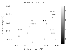
Figure 2: Train vs. test performance for different margins $\rho$ on instance australian. Each point represents a solution encountered by IPBoost while solving the boosting problem. Grayscale values indicate the number of base learners used in boosted learners; see the legend.

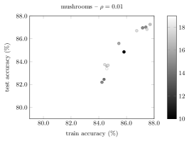
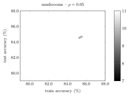
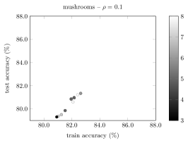
Figure 3: Train vs. test performance for different margins $\rho$ on instance mushrooms. Each point represents a solution encountered by IPBoost while solving the boosting problem. Grayscale values indicate the number of base learners used in boosted learners; see the legend.

References

- [1] C. Barnhart, E. L. Johnson, G. L. Nemhauser, M. W. P. Savelsbergh, and P. H. Vance. Branch-and-price: Column generation for solving huge integer programs. Oper. Res., 46(3):316–329, 1998.
- [2] T. Berthold. Heuristic algorithms in global MINLP solvers. PhD thesis, TU Berlin, 2014.
- [3] D. Bertsimas and J. Dunn. Optimal classification trees. Machine Learning, pages 1–44, 2017.
- [4] D. Bertsimas and A. King. OR forum—an algorithmic approach to linear regression. Operations Research, 64(1):2–16, 2015.
- [5] D. Bertsimas, A. King, R. Mazumder, et al. Best subset selection via a modern optimization lens. The Annals of Statistics, 44(2):813–852, 2016.
- [6] D. Bertsimas and R. Shioda. Classification and regression via integer optimization. Operations Research, 55(2):252–271, 2007.
- [7] R. Borndörfer, A. Löbel, M. Reuther, T. Schlechte, and S. Weider. Rapid branching. Public Transport, 5(1):3–23, 2013.
- [8] R. Borndörfer, A. Löbel, and S. Weider. A bundle method for integrated multi-depot vehicle and duty scheduling in public transit. In M. Hickman, P. Mirchandani, and S. Voß, editors, Computer-aided Systems in Public Transport, volume 600, pages 3–24, 2008.
- [9] L. Breiman. Bagging predictors. Machine Learning, 24:123–140, 1996.
- [10] A. Chang, D. Bertsimas, and C. Rudin. An integer optimization approach to associative classification. In Advances in Neural Information Processing Systems, pages 269–277, 2012.
- [11] C. Cortes, M. Mohri, and U. Syed. Deep boosting. In 31st International Conference on Machine Learning, ICML 2014. International Machine Learning Society (IMLS), 2014.
- [12] CPLEX. IBM ILOG CPLEX Optimizer. https://www.ibm.com/analytics/cplex-optimizer, 2020.
- [13] S. Dash, O. Günlük, and D. Wei. Boolean decision rules via column generation. In Advances in Neural Information Processing Systems, pages 4655–4665, 2018.
- [14] A. Demiriz, K. P. Bennett, and J. Shawe-Taylor. Linear programming boosting via column generation. Machine Learning, 46(1-3):225–254, 2002.
- [15] J. Desrosiers and M. E. Lübbecke. A primer in column generation. In Column generation, pages 1–32. Springer, 2005.
- [16] J. Eckstein and N. Goldberg. An improved branch-and-bound method for maximum monomial agreement. INFORMS Journal on Computing, 24(2):328–341, 2012.
- [17] M. Fischetti and J. Jo. Deep neural networks and mixed integer linear optimization. Constraints, 23(3):296–309, 2018.
- [18] R. M. Freund, P. Grigas, and R. Mazumder. A new perspective on boosting in linear regression via subgradient optimization and relatives. arXiv preprint arXiv:1505.04243, 2015.
- [19] Y. Freund and R. E. Schapire. A desicion-theoretic generalization of on-line learning and an application to boosting. In European Conference on Computational Learning Theory, pages 23–37. Springer, 1995.
- [20] A. Gleixner, M. Bastubbe, L. Eifler, T. Gally, G. Gamrath, R. L. Gottwald, G. Hendel, C. Hojny, T. Koch, M. E. Lübbecke, S. J. Maher, M. Miltenberger, B. Müller, M. E. Pfetsch, C. Puchert, D. Rehfeldt, F. Schlösser, C. Schubert, F. Serrano, Y. Shinano, J. M. Viernickel, M. Walter, F. Wegscheider, J. T. Witt, and J. Witzig. The SCIP Optimization Suite 6.0. Technical report, Optimization Online, July 2018.
- [21] N. Goldberg and J. Eckstein. Boosting classifiers with tightened l0-relaxation penalties. In Proceedings of the 27th International Conference on Machine Learning (ICML-10), pages 383–390, 2010.
- [22] N. Goldberg and J. Eckstein. Sparse weighted voting classifier selection and its linear programming relaxations. Information Processing Letters, 112(12):481–486, 2012.
- [23] O. Günlük, J. Kalagnanam, M. Menickelly, and K. Scheinberg. Optimal generalized decision trees via integer programming. arXiv preprint arXiv:1612.03225, 2016.
- [24] O. Günlük, J. Kalagnanam, M. Menickelly, and K. Scheinberg. Optimal decision trees for categorical data via integer programming. arXiv preprint arXiv:1612.03225, 2018.
- [25] Gurobi. Gurobi Optimizer. http://www.gurobi.com, 2020.
- [26] J. Leskovec and J. Shawe-Taylor. Linear programming boosting for uneven datasets. In Proceedings of the Twentieth International Conference on Machine Learning (ICML-2003), pages 456–463, 2003.
- [27] P. M. Long and R. A. Servedio. Random classification noise defeats all convex potential boosters. In Proceedings of the 25th international conference on Machine learning, pages 608–615. ACM, 2008.
- [28] P. M. Long and R. A. Servedio. Random classification noise defeats all convex potential boosters. Machine learning, 78(3):287–304, 2010.
- [29] F. Pedregosa, G. Varoquaux, A. Gramfort, V. Michel, B. Thirion, O. Grisel, M. Blondel, P. Prettenhofer, R. Weiss, V. Dubourg, et al. Scikit-learn: Machine learning in python. Journal of Machine Learning Research, 12(Oct):2825–2830, 2011.
- [30] M. E. Pfetsch. Branch-and-cut for the maximum feasible subsystem problem. SIAM J. Optim., 19(1):21–38, 2008.
- [31] P. Savickỳ, J. Klaschka, and J. Antoch. Optimal classification trees. In COMPSTAT, pages 427–432. Springer, 2000.
- [32] R. E. Schapire. The boosting approach to machine learning: An overview. In Nonlinear estimation and classification, pages 149–171. Springer, 2003.
- [33] S. Shalev-Shwartz and Y. Wexler. Minimizing the maximal loss: How and why. In Proceedings of the 32nd International Conference on Machine Learning, 2016.
- [34] V. Tjeng, K. Xiao, and R. Tedrake. Evaluating robustness of neural networks with mixed integer programming. arXiv preprint arXiv:1711.07356, 2017.
- [35] S. Verwer and Y. Zhang. Learning optimal classification trees using a binary linear program formulation. In 33rd AAAI Conference on Artificial Intelligence, 2019.
- [36] XPRESS. FICO Xpress Optimizer. https://www.fico.com/en/products/fico-xpress-optimization, 2020.
- [37] J. Zhu, H. Zou, S. Rosset, and T. Hastie. Multi-class adaboost. Statistics and its Interface, 2(3):349–360, 2009.
Supplementary Material