Object Detection as a
Positive-Unlabeled Problem

Abstract

As with other deep learning methods, label quality is important for learning modern convolutional object detectors. However, the potentially large number and wide diversity of object instances that can be found in complex image scenes makes constituting complete annotations a challenging task. Indeed, objects missing annotations can be observed in a variety of popular object detection datasets. These missing annotations can be problematic, as the standard cross-entropy loss employed to train object detection models treats classification as a positive-negative (PN) problem: unlabeled regions are implicitly assumed to be background. As such, any object missing a bounding box results in a confusing learning signal, the effects of which we observe empirically. To remedy this, we propose treating object detection as a positive-unlabeled (PU) problem, which removes the assumption that unlabeled regions must be negative. We demonstrate that our proposed PU classification loss outperforms the standard PN loss on PASCAL VOC and MS COCO across a range of label missingness, as well as on Visual Genome and DeepLesion with full labels.

1 Introduction

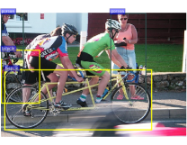
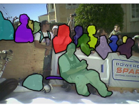
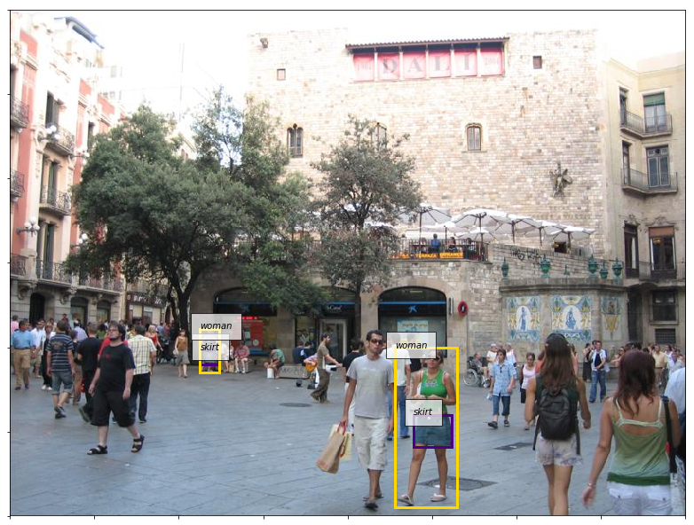
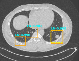
Figure 1: Because of the inherent difficulty of instance labeling, the ground truth of object detection datasets can be incomplete. Example images and their ground truth labels shown for (left to right) PASCAL VOC [Everingham et al.(2010)Everingham, Van Gool, Williams, Winn, and Zisserman] (missing people, bottles), MS COCO [Lin et al.(2014)Lin, Maire, Belongie, Bourdev, Girshick, Hays, Perona, Ramanan, Zitnick, and Dolí] (missing people), Visual Genome [Krishna et al.(2017)Krishna, Zhu, Groth, Johnson, Hata, Kravitz, Chen, Kalantidis, Li, Shamma, Bernstein, and Fei-Fei] (missing people, tree, clothing, etc.), and DeepLesion [Yan et al.(2017)Yan, Wang, Lu, and Summers] (ground truth is the dotted line; two boxes on the left indicate two unlabeled nodules).

The performance of supervised deep learning models is often highly dependent on the quality of the labels they are trained on [Zhang et al.(2017)Zhang, Bengio, Brain, Hardt, Recht, Vinyals, and Deepmind, Veit et al.(2017)Veit, Alldrin, Chechik, Krasin, Gupta, and Belongie, Jiang et al.(2018)Jiang, Zhou, Leung, Li, and Fei-Fei]. Recent work by [Toneva et al.(2019)Toneva, Sordoni, des Combes, Trischler, Bengio, and Gordon] has implied the existence of “support vectors” in datasets: hard to classify examples that have an especially significant influence on a classifier’s decision boundary. As such, ensuring that these difficult examples have the correct label would appear to be important to the final classifier. However, collecting complete labels for object detection [Girshick et al.(2014)Girshick, Donahue, Darrell, and Malik, Girshick(2015), Liu et al.(2016)Liu, Anguelov, Erhan, Szegedy, Reed, Fu, and Berg, Ren et al.(2015)Ren, He, Girshick, and Sun, Redmon et al.(2016)Redmon, Divvala, Girshick, and Farhadi, Dai et al.(2016)Dai, Li, He, and Sun, Redmon and Farhadi(2017)] can be challenging, much more so than for classification tasks. Unlike the latter, with a single label per image, the number of objects in an image is often variable, and objects can come in a large variety of shapes, sizes, poses, and settings, even within the same class. Furthermore, object detection scenes are often crowded, resulting in object instances that may be occluded. Given the requirement for tight bounding boxes and the sheer number of instances to label, constituting annotations can be very time-consuming. For example, just labeling instances, without localization, required $\sim$30K worker hours for the 328K images of MS COCO [Lin et al.(2014)Lin, Maire, Belongie, Bourdev, Girshick, Hays, Perona, Ramanan, Zitnick, and Dolí], and the airport checkpoint X-ray dataset used in [Liang et al.(2018)Liang, Heilmann, Gregory, Diallo, Carlson, Spell, Sigman, Roe, and Carin, Sigman et al.(2020)Sigman, Spell, Liang, and Carin], which required assembling bags, scanning, and hand labeling, took over 250 person hours for 4000 scans over the span of several months. For medical datasets [Moreira et al.(2012)Moreira, Amaral, Domingues, Cardoso, Cardoso, and Cardoso, Yan et al.(2017)Yan, Wang, Lu, and Summers, Lee et al.(2017)Lee, Gimenez, Hoogi, Miyake, Gorovoy, and Rubin, Wang et al.(2017)Wang, Peng, Lu, Lu, Bagheri, and Summers], this becomes even more problematic, as highly trained (and expensive) radiologist experts or invasive biopsies are needed to determine ground truth.

As a result of its time-consuming nature, dataset annotations are often crowd-sourced when possible, either with specialized domain experts or Amazon Mechanical Turk. In order to ensure consistency, dataset designers establish labeling guidelines or have multiple workers label the same image [Everingham et al.(2010)Everingham, Van Gool, Williams, Winn, and Zisserman, Lin et al.(2014)Lin, Maire, Belongie, Bourdev, Girshick, Hays, Perona, Ramanan, Zitnick, and Dolí]. Regardless, tough judgment calls, inter- and even intra-worker variability, and human error can still result in overall inconsistency in labeling, or missing instances entirely. This becomes especially exacerbated when establishing a larger dataset, like OpenImages [Kuznetsova et al.(2018)Kuznetsova, Rom, Alldrin, Uijlings, Krasin, Pont-Tuset, Kamali, Popov, Malloci, Duerig, and Ferrari], which while extremely large, is incompletely labeled.

Despite this, object detection algorithms often use the standard cross-entropy loss for object classification. Implicit to this loss function is the assumption that any region without a bounding box does not contain an object; in other words, classification is posed as a positive-negative (PN) learning problem. While reasonable for a completely labeled dataset, despite best efforts, this is often not the case in practice due to the previously outlined difficulties of instance annotations. As shown in Figure 1 for a wide array of common datasets, the lack of instance labels does not always mean the absence of true objects.

While the result of this characterization constitutes a noisy label setting, it is not noisy in the same respect as is commonly considered for classification problems [Zhang et al.(2017)Zhang, Bengio, Brain, Hardt, Recht, Vinyals, and Deepmind, Veit et al.(2017)Veit, Alldrin, Chechik, Krasin, Gupta, and Belongie, Jiang et al.(2018)Jiang, Zhou, Leung, Li, and Fei-Fei]. The presence of a positive label in object detection datasets are generally correct with high probability; it is the lack of a label that should not be interpreted with confidence as a negative (or background) region. Thus, given these characteristics common to object detection data, we propose recasting object detection as a positive-unlabeled (PU) learning problem [Denis(1998), De Comité et al.(1999)De Comité, Denis, Gilleron, and Letouzey, Letouzey et al.(2000)Letouzey, Denis, and Gilleron, Elkan and Noto(2008), Kiryo et al.(2017)Kiryo, Niu, Du Plessis, and Sugiyama]. With such a perspective, existing labels still implies a positive sample, but the lack of one no longer enforces that the region must be negative. This can mitigate the confusing learning signal that often occurs when training on object detection datasets.

In this work, we explore how the characteristics of object detection annotation lend themselves to a PU learning problem and demonstrate the efficacy of adapting detection model training objectives accordingly. We perform a series of experiments to demonstrate the effectiveness of the PU objective on two popular, well-labeled object detection datasets (PASCAL VOC [Everingham et al.(2010)Everingham, Van Gool, Williams, Winn, and Zisserman] and MS COCO [Lin et al.(2014)Lin, Maire, Belongie, Bourdev, Girshick, Hays, Perona, Ramanan, Zitnick, and Dolí]) across a range of label missingness, as well as two datasets with real incomplete labels (Visual Genome [Krishna et al.(2017)Krishna, Zhu, Groth, Johnson, Hata, Kravitz, Chen, Kalantidis, Li, Shamma, Bernstein, and Fei-Fei], DeepLesion [Yan et al.(2017)Yan, Wang, Lu, and Summers]).

2 Methods

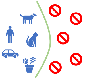
(a) Positive-Negative, with full labels

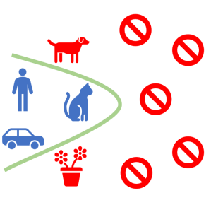
(b) Positive-Negative, with missing labels

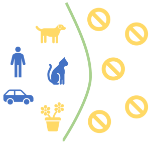
(c) Positive-Unlabeled

Figure 2: A classifier (green) learns to separate proposals by “objectness”. Models trained with a standard cross-entropy loss implicitly assume positive-negative (PN) learning: regions with bounding boxes are considered positive (blue), and any other proposed boxes are treated as negative (red). This is reasonable when labels are complete (a), but in reality, object detection datasets are inherently missing annotations; this forces the classifier to exclude unlabeled objects from the positive class (b). We propose a positive-unlabeled (PU) approach (c), which considers non-labeled regions as unlabeled (yellow) rather than negative, allowing non-positive regions to be classified as positive. Best viewed in color.

2.1 Faster R-CNN

In principle, the observed problem is characteristic of the data and is thus general to any object detection framework. However, in this work, we primarily focus on Faster R-CNN [Ren et al.(2015)Ren, He, Girshick, and Sun], a popular 2-stage method for which we provide a quick overview here.

As with other object detection models, given an input image $X$, the desired output of Faster R-CNN is a bounding box $B^{(i)}\in\mathbb{R}^{4}$ and class probabilities $c^{(i)}\in\mathbb{R}^{k}$ for each object (indexed by $i$) present, where $k$ is the number of classes and the final classification decision is commonly $\operatorname*{arg\!\max}c^{(i)}$. Faster R-CNN does this in a 2-stage process. First, a convolutional neural network (CNN) [Lecun et al.(1989)Lecun, Boser, Denker, Henderson, Howard, Hubbard, and Jackel] is used to produce image features $h$. A Region Proposal Network (RPN) then generates bounding box proposals $\hat{B}^{(i)}$ relative to a set of reference boxes spatially tiled over $h$. At the same time, the RPN predicts an “objectness” probability $\hat{c}^{(i)}$ for each proposal, learned as an object-or-not binary classifier. The second stage then takes the proposals with the highest scores, and predicts bounding box refinements to produce $B^{(i)}$ and the final classification probabilities $c^{(i)}$.

Of particular interest is how the classifier producing $\hat{c}^{(i)}$ is trained. Specifically, the cross-entropy loss $H(t,y)$ is employed, where $H(t,y)$ signifies the loss incurred when the model outputs $t$ when the ground truth is $y$. In the RPN, this results in the following classification risk minimization:

$$R^{RPN}_{pn}=\pi_{p}\mathbb{E}[H(\hat{c}_{p},+1)]+\pi_{n}\mathbb{E}[H(\hat{c}_{n},-1)]$$ (1)

where $\pi_{p}$ and $\pi_{n}$ are the class probability priors for the positive and negative classes, respectively, and $\hat{c}^{(i)}_{p}$ and $\hat{c}^{(i)}_{n}$ are the predicted “objectness” probabilities for ground truth positive and negative regions. This risk is estimated with samples as:

$$\mathcal{L}^{RPN}_{pn}=\frac{\hat{\pi}_{p}}{N_{p}}\sum_{i=1}^{N_{p}}H(\hat{c}^{(i)}_{p},+1)+\frac{\hat{\pi}_{n}}{N_{n}}\sum_{i=1}^{N_{n}}H(\hat{c}^{(i)}_{n},-1)$$ (2)

where $N_{p}$ and $N_{n}$ are the number of ground truth positive and negative regions being considered, respectively, and the class priors are typically estimated as $\hat{\pi}_{p}=\frac{N_{p}}{N_{p}+N_{n}}$ and $\hat{\pi}_{n}=\frac{N_{n}}{N_{p}+N_{n}}$. Notably, this training loss treats all non-positive regions in an image as negative.

2.2 PU learning

In a typical binary classification problem, input data $X\in\mathbb{R}^{d}$ are labeled as $Y\in\{\pm 1\}$, resulting in what is commonly termed a positive-negative (PN) problem. This implicitly assumes having samples from both the positive (P) and negative (N) distributions, and that these samples are labeled correctly (Figure 2a). However, in some scenarios, we only have labels for some positive samples. The remainder of our data are unlabeled (U): samples that could be positive or negative. Such a situation is called a positive-unlabeled (PU) setting, where the N distribution is replaced by an unlabeled (U) distribution (Figure 2c). Such a representation admits a classifier that can appropriately include unlabeled positive regions on the correct side of the decision boundary. We briefly review PN and PU risk estimation here.

Let $p(x,y)$ be the underlying joint distribution of $(X,Y)$, $p_{p}(x)=p(x|Y=+1)$ and $p_{n}(x)=p(x|Y=-1)$ be the distributions of P and N data, $p(x)$ be the distribution of U data, $\pi_{p}=p(Y=+1)$ be the positive class-prior probability, and $\pi_{n}=p(Y=-1)=1-\pi_{p}$ be the negative class-prior probability. In a PN setting, data are sampled from $p_{p}(x)$ and $p_{n}(x)$ such that $\mathcal{X}_{p}=\{x^{p}_{i}\}^{N_{p}}_{i=1}\sim{p_{p}(x)}$ and $\mathcal{X}_{n}=\{x^{n}_{i}\}^{N_{n}}_{i=1}\sim{p_{n}(x)}$. Let $g$ be an arbitrary decision function that represents a model. The risk of $g$ can be estimated from $\mathcal{X}_{p}$ and $\mathcal{X}_{n}$ as:

$$\hat{R}_{pn}(g)=\pi_{p}\hat{R}^{+}_{p}(g)+\pi_{n}\hat{R}^{-}_{n}(g)$$ (3)

$\hat{R}^{+}_{p}(g)=1/N_{p}\sum^{N_{p}}_{i=1}\ell(g(x^{p}_{i}),+1)$ and $\hat{R}^{-}_{n}(g)=1/N_{n}\sum^{N_{n}}_{i=1}\ell(g(x^{n}_{i}),-1)$, where $\ell$ is the loss function. In classification, $\ell$ is commonly the cross-entropy loss $H(t,y)$.

In PU learning, $\mathcal{X}_{n}$ is unavailable; instead we have unlabeled data $\mathcal{X}_{u}=\{x^{u}_{i}\}^{N_{u}}_{i=1}\sim{p(x)}$, where $N_{u}$ is the number of unlabeled samples. However, the negative class empirical risk $\hat{R}^{-}_{n}(g)$ in Equation 3 can be approximated indirectly [Du Plessis et al.(2015)Du Plessis, Niu, and Sugiyama, Du Plessis et al.(2014)Du Plessis, Niu, and Sugiyama]. Denoting $R^{-}_{p}(g)=\mathbb{E}_{p}[\ell(g(X),-1)]$ and $R^{-}_{u}(g)=\mathbb{E}_{X\sim{p(x)}}[\ell(g(X),-1)]$, and observing $\pi_{n}p_{n}(x)=p(x)-\pi_{p}p_{p}(x)$, we can replace the missing term $\pi_{n}R_{n}^{-}(g)=R^{-}_{u}(g)-\pi_{p}R^{-}_{p}(g)$. Hence, we express the overall risk without explicit negative data as

$$\hat{R}_{pu}(g)=\pi_{p}\hat{R}^{+}_{p}(g)+\hat{R}^{-}_{u}(g)-\pi_{p}\hat{R}^{-}_{p}(g)$$ (4)

where $\hat{R}^{-}_{p}(g)=1/N_{p}\sum^{N_{p}}_{i=1}\ell(g(x^{p}_{i}),-1)$ and $\hat{R}^{-}_{u}(g)=1/N_{u}\sum^{N_{u}}_{i=1}\ell(g(x^{u}_{i}),-1)$.

However, a flexible enough model can overfit the data, leading to the empirical risk in Equation 4 becoming negative. Given that most modern object detectors utilize neural networks, this type of overfitting can pose a significant problem. In [Kiryo et al.(2017)Kiryo, Niu, Du Plessis, and Sugiyama], the authors propose a non-negative PU risk estimator to combat this:

$$\hat{R}_{pu}(g)=\pi_{p}\hat{R}^{+}_{p}(g)+\max\{0,\hat{R}^{-}_{u}(g)-\pi_{p}\hat{R}^{-}_{p}(g)\}$$ (5)

We choose to employ this non-negative PU risk estimator for the rest of this work.

2.3 PU learning for object detection

2.3.1 PU object proposals

In object detection datasets, the ground truth labels represent positive samples. Any regions that do not share sufficient overlap with a ground truth bounding box are typically considered as negative background, but the accuracy of this assumption depends on every object within a training image being labeled, which may not be the case (Figure 1). As shown in Figure 2b, this results in the possibility of positive regions being proposed that are labeled negative during training, due to a missing ground truth label; effects of this phenomenon during training are investigated empirically in Supplementary Materials Section A. We posit that object detection more naturally resembles a PU learning problem than PN.

We recognize that two-stage detection naturally contains a binary classification problem in the first stage. In Faster R-CNN specifically, the RPN assigns an “objectness” score, which is learned with a binary cross-entropy loss (Equation 2). As previously noted, the PN nature of this loss can be problematic, so we propose replacing it with a PU formulation. Combining Equations 2 and 5, we produce the following loss function:

$$\mathcal{L}^{RPN}_{pu}=\frac{\pi_{p}}{N_{p}}\sum_{i=1}^{N_{p}}H(\hat{c}^{(i)}_{p},+1)+\max\bigg{\{}0,\frac{1}{N_{u}}\sum_{i=1}^{N_{u}}H(\hat{c}^{(i)}_{u},-1)-\frac{\pi_{p}}{N_{p}}\sum_{i=1}^{N_{p}}H(\hat{c}^{(i)}_{p},-1)\bigg{\}}$$ (6)

Such a loss function relaxes the penalty of positive predictions for unlabeled objects.

2.3.2 Estimating $\pi_{p}$

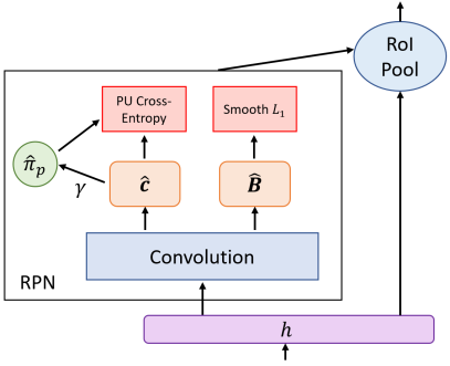
Figure 3: Faster R-CNN [Ren et al.(2015)Ren, He, Girshick, and Sun] RPN with the proposed PU cross-entropy loss. Positive class prior estimate $\hat{\pi}_{p}$ is updated with objectness predictions $\hat{c}$, with momentum $\gamma$.

The PU cross-entropy loss in Equation 6 assumes the class-prior probability of the positive class $\pi_{p}$ is known. In practice, this is not usually the case, so $\pi_{p}$ must be estimated, denoted as $\hat{\pi}_{p}$. For object detection, estimating $\pi_{p}$ is especially problematic because $\pi_{p}$ is not static: as the RPN is trained, an increasing proportion of region proposals will (hopefully) be positive. While [Kiryo et al.(2017)Kiryo, Niu, Du Plessis, and Sugiyama] showed some robustness to $\pi_{p}$ misspecification, this was only on a fairly narrow range of $\pi_{p}\in[0.8\pi_{p},1.2\pi_{p}]$. During object detection performance, $\pi_{p}$ starts from virtually $0$ and grows steadily as the RPN improves. As such, any single estimate $\hat{\pi}_{p}$ poses the risk of being significantly off the mark during a large portion of training.

To address this, we recognize that the RPN of Faster R-CNN is already designed to infer the positive regions of an image, so we count the number of positive regions produced by the RPN and use it as an estimator for $\pi_{p}$:

$$\hat{\pi}_{p}=\frac{N_{p}^{RPN}}{N^{RPN}}$$ (7)

where $N^{RPN}$ is the total number of RPN proposals that are sampled for training, and $N_{p}^{RPN}$ being those with classifier confidence of at least 0.5. Note that this estimation of $\pi_{p}$ comes essentially for free. Given that Faster R-CNN is trained one image at a time and the prevalence of objects varies between images, we maintain an exponential moving average with momentum $\gamma$ in order to stabilize $\hat{\pi}_{p}$ (see Figure 3). This estimate $\hat{\pi}_{p}$ is then used in the calculation of the loss $\mathcal{L}^{RPN}_{pu}$ and its gradients.

3 Related work

Most object detection frameworks are designed fully supervised [Girshick et al.(2014)Girshick, Donahue, Darrell, and Malik, Girshick(2015), Liu et al.(2016)Liu, Anguelov, Erhan, Szegedy, Reed, Fu, and Berg, Ren et al.(2015)Ren, He, Girshick, and Sun, Redmon et al.(2016)Redmon, Divvala, Girshick, and Farhadi, Dai et al.(2016)Dai, Li, He, and Sun, Redmon and Farhadi(2017)]: it is assumed that there exists a dataset of images where every object is labeled and such a dataset is available to train the model. However, as discussed above, collecting such a dataset can be expensive. Because of this, methods that can learn from partially labeled datasets have been a topic of interest for object detection. What “partially labeled” constitutes can vary, and many types of label missingness have been considered.

Weakly supervised object detection models [Bilen and Vedaldi(2016), Oquab et al.(2015)Oquab, Bottou, Laptev, and Sivic, Rochan and Wang(2015)] assume a dataset with image level labels, but without instance labels. These models are somewhat surprisingly competent at identifying approximate locations of objects in an image without any object-specific cues, but have a harder time with precise localization. This is especially the case when there are many of the same class of object in close proximity to each other, as individual activations can blur together, and the lack of bounding boxes makes it difficult to learn precise boundaries. Other approaches consider settings where bounding boxes are available for some classes (e.g., PASCAL VOC’s 20 classes) but not others (e.g., ImageNet [Deng et al.(2009)Deng, Dong, Socher, Li, Li, and Li] classes). LSDA [Hoffman et al.(2014)Hoffman, Guadarrama, Tzeng, Donahue, Girshick, Darrell, and Saenko] does this by modifying the final layer of a CNN [Krizhevsky et al.(2012)Krizhevsky, Sutskever, and Hinton] to recognize classes from both categories, and [Tang et al.(2016)Tang, Wang, Gao, Dellandrea, Gaizauskas, and Chen] improves upon LSDA by taking advantage of visual and semantic similarities between classes. OMNIA [Rame et al.(2018)Rame, Garreau, Ben-Younes, and Ollion] proposes a method merging datasets that are each fully annotated for their own set of classes, but not each other’s.

There are also approaches that consider a single dataset, but the labels are undercomplete across all classes. This setting most resembles what we consider in our paper. In [Dong et al.(2018)Dong, Zheng, Ma, Yang, and Meng], only 3-4 annotated examples per class are assumed given to start; additional pseudo-labels are generated from the model on progressively more difficult examples as the model improves. Soft-sampling has also been proposed to re-weight gradients of background regions that either have overlap with positive regions or produce high detection scores in a separately trained detector [Wu et al.(2019)Wu, Bodla, Singh, Najibi, Chellappa, and Davis]; experiments were done on PASCAL VOC with a percentage of annotations discarded and on a subset of OpenImages [Kuznetsova et al.(2018)Kuznetsova, Rom, Alldrin, Uijlings, Krasin, Pont-Tuset, Kamali, Popov, Malloci, Duerig, and Ferrari].

Positive-unlabeled learning has been proposed to improve statistical models with limited labeled data [Lee and Liu(2003), Letouzey et al.(2000)Letouzey, Denis, and Gilleron]. [Kiryo et al.(2017)Kiryo, Niu, Du Plessis, and Sugiyama, Xu et al.(2017)Xu, Xu, Xu, and Tao] analyzed the theoretical effectiveness of positive-unlabeled risk estimation on binary classification tasks, though with the proportion of positive class examples preset and known to the model. [Jain et al.(2016)Jain, White, and Radivojac, Du Plessis et al.(2014)Du Plessis, Niu, and Sugiyama] infer the positive class prior with additional classifiers or matching algorithms. Our work extends the application of positive-unlabeled learning to alleviate the incomplete labels that can be found in most object detection datasets.

4 Experiments

For our experiments, we use the original Faster-RCNN [Ren et al.(2015)Ren, He, Girshick, and Sun], with a ResNet101 [He et al.(2016)He, Zhang, Ren, and Sun] feature extractor (without feature pyramid network [Lin et al.(2017)Lin, Dollár, Girshick, He, Hariharan, and Belongie]) pre-trained on ImageNet [Deng et al.(2009)Deng, Dong, Socher, Li, Li, and Li]. To control the level of missingness of each dataset, each annotation from a object class provided by original dataset is randomly discarded with a probability $\rho$. This effectively makes the available annotations to be $1-\rho$ of total annotations on average.

4.1 Hand-tuning versus estimation of $\pi_{p}$

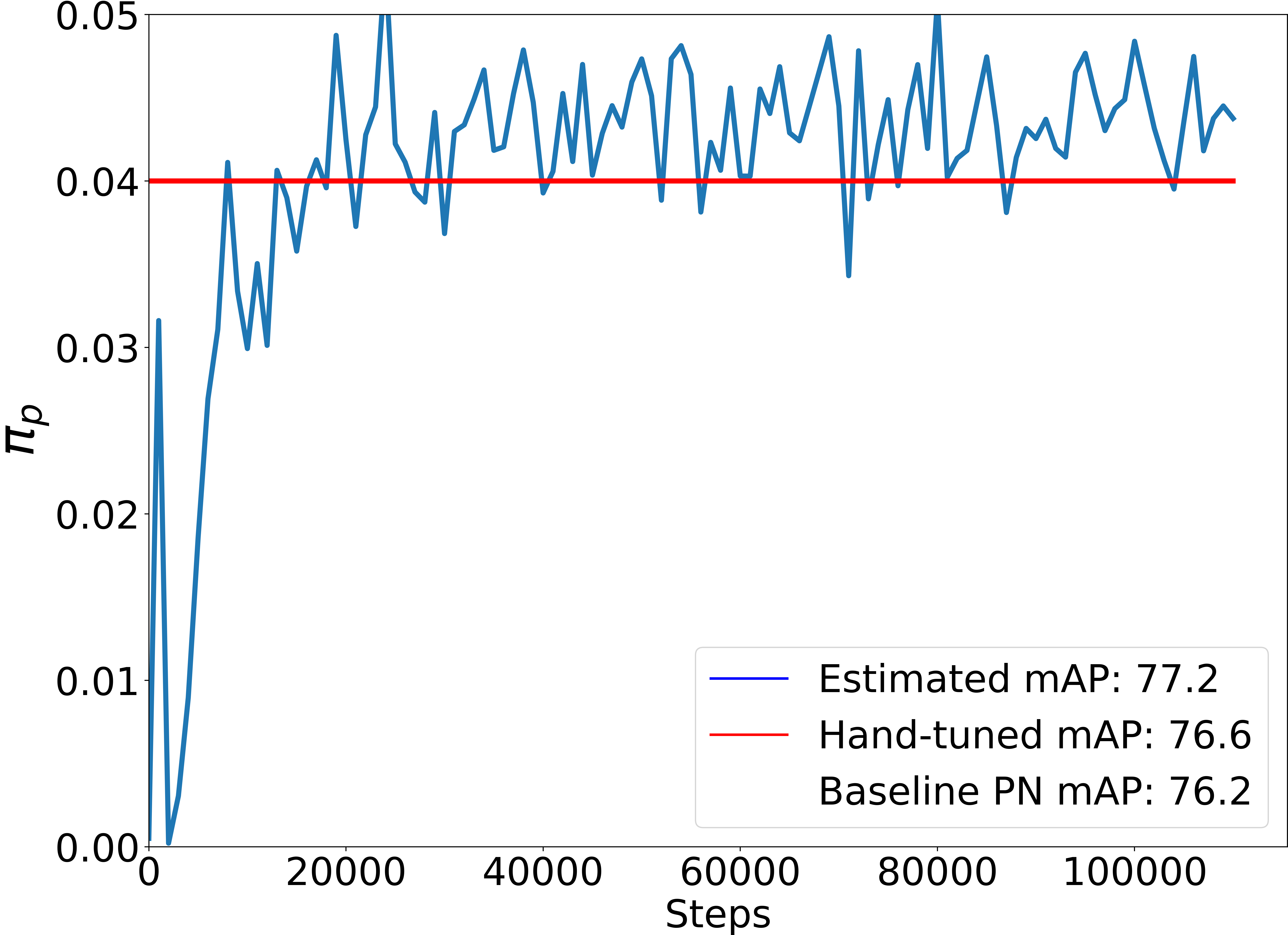
(a) $\rho=0.4$

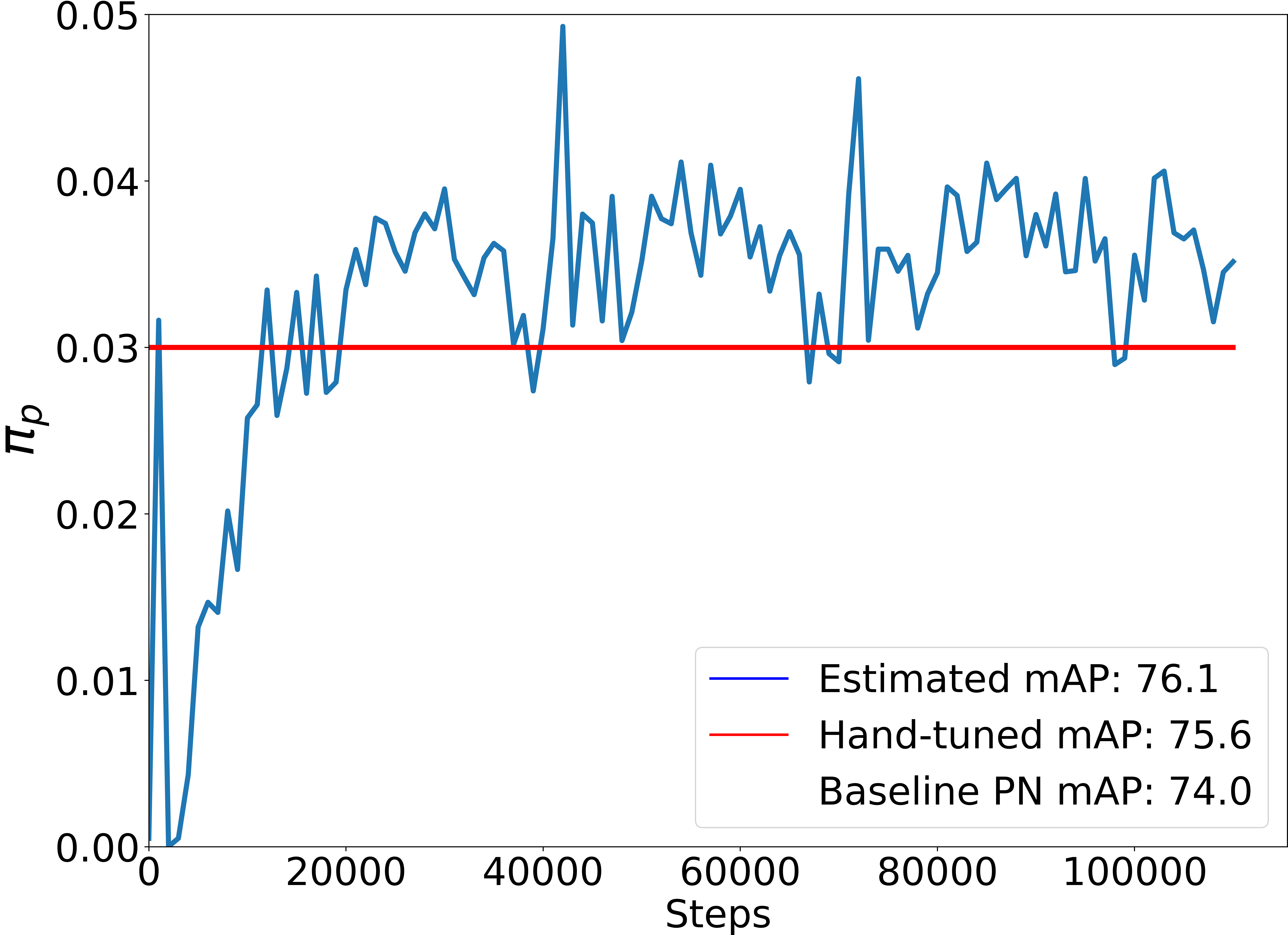
(b) $\rho=0.5$

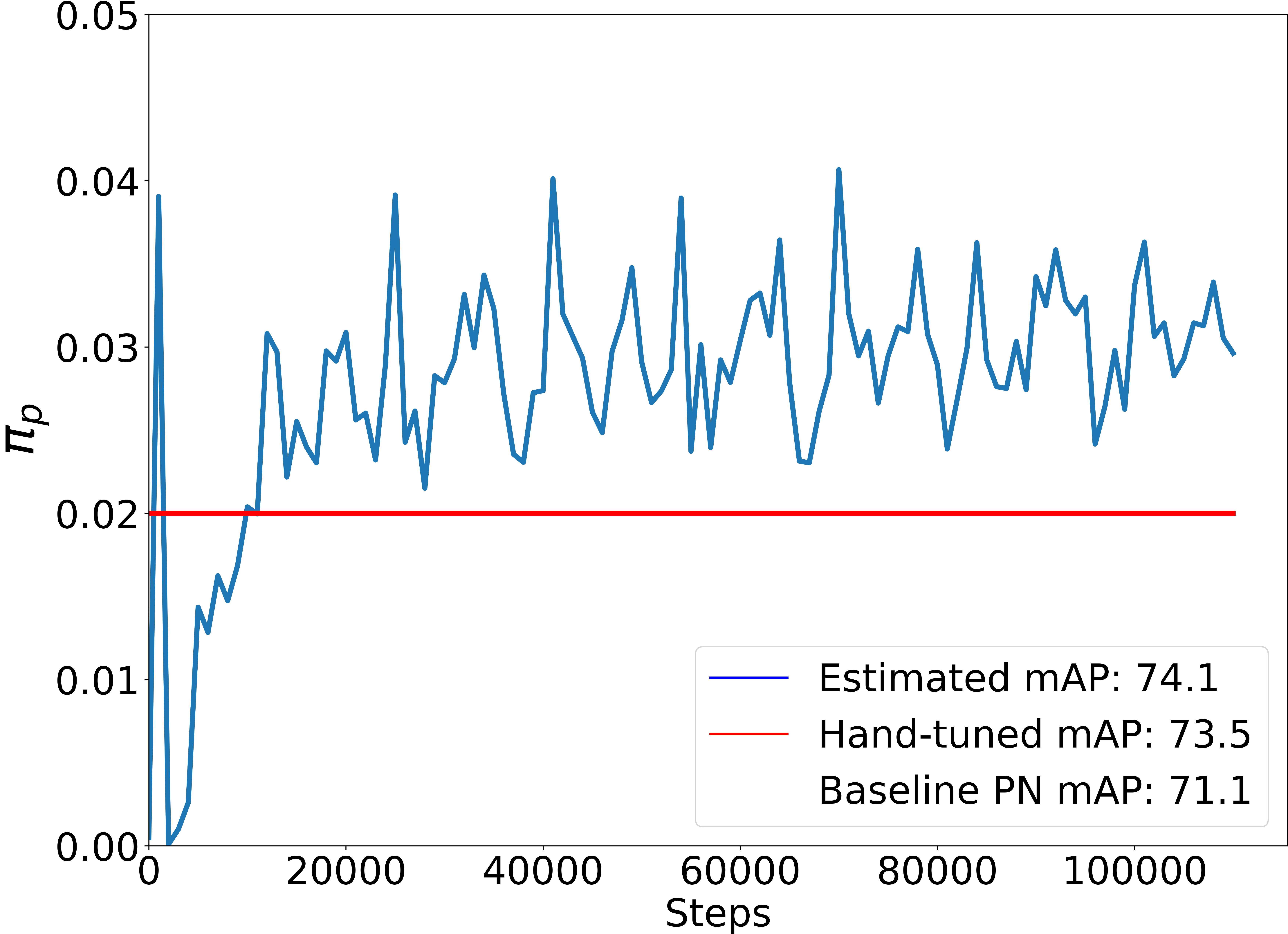
(c) $\rho=0.6$

Figure 4: Positive class prior $\hat{\pi}_{p}$ estimated during training of Faster R-CNN on PASCAL VOC versus from hand-tuning $\pi_{p}$ as a hyperparameter, for instance label missingness proportion $\rho=\{0.4,0.5,0.6\}$.

As discussed in Section 2.3.2, PU risk estimation requires the prior $\pi_{p}$. We experiment with two ways of determining $\pi_{p}$. In the first method (Hand-Tuned), we treat $\pi_{p}$ as a constant hyperparameter and tune it by hand. In the second (Estimated), we infer $\pi_{p}$ as described in Equation 7, setting momentum $\gamma$ to 0.9. We compare the estimate $\hat{\pi}_{p}$ inferred automatically with the hand-tuned $\pi_{p}$ that yielded the highest mAP on PASCAL VOC. To see how our estimate changes in response to label missingness, when assembling our training set, we remove each annotation from an image with probability $\rho$, giving us a dataset with $1-\rho$ proportion of the total labels, and then do our comparison for $\rho=\{0.4,0.5,0.6\}$ in Figure 4.

In all tested settings of $\rho$, the estimation $\hat{\pi}_{p}$ increases over time before stabilizing. Such a result matches expectations, as when an object detection model is first initialized, its parameters have yet to learn good values, and thus the true proportion of positive regions $\pi_{p}$ is likely to be quite low. As the model trains, its ability to generate accurate regions improves, resulting in a higher proportion of regions being positive. This in turn results in a higher true value of $\pi_{p}$, which our estimate $\hat{\pi}_{p}$ follows. As the model converges, $\pi_{p}$ (and $\hat{\pi}_{p}$) stabilizes towards the true prevalence of objects in the dataset relative to background regions. Interestingly, the final value of $\hat{\pi}_{p}$ settles close to the value of $\pi_{p}$ found by treating the positive class prior as a static hyperparameter, but consistently above it. We hypothesize that this is due to a single static value having to hedge against the early stages of training, when $\pi_{p}$ is lower. We use our proposed method of auto-inferring $\pi_{p}$ for the rest of our experiments, with $\gamma=0.9$, rather than hand-tuning it as a hyperparameter.

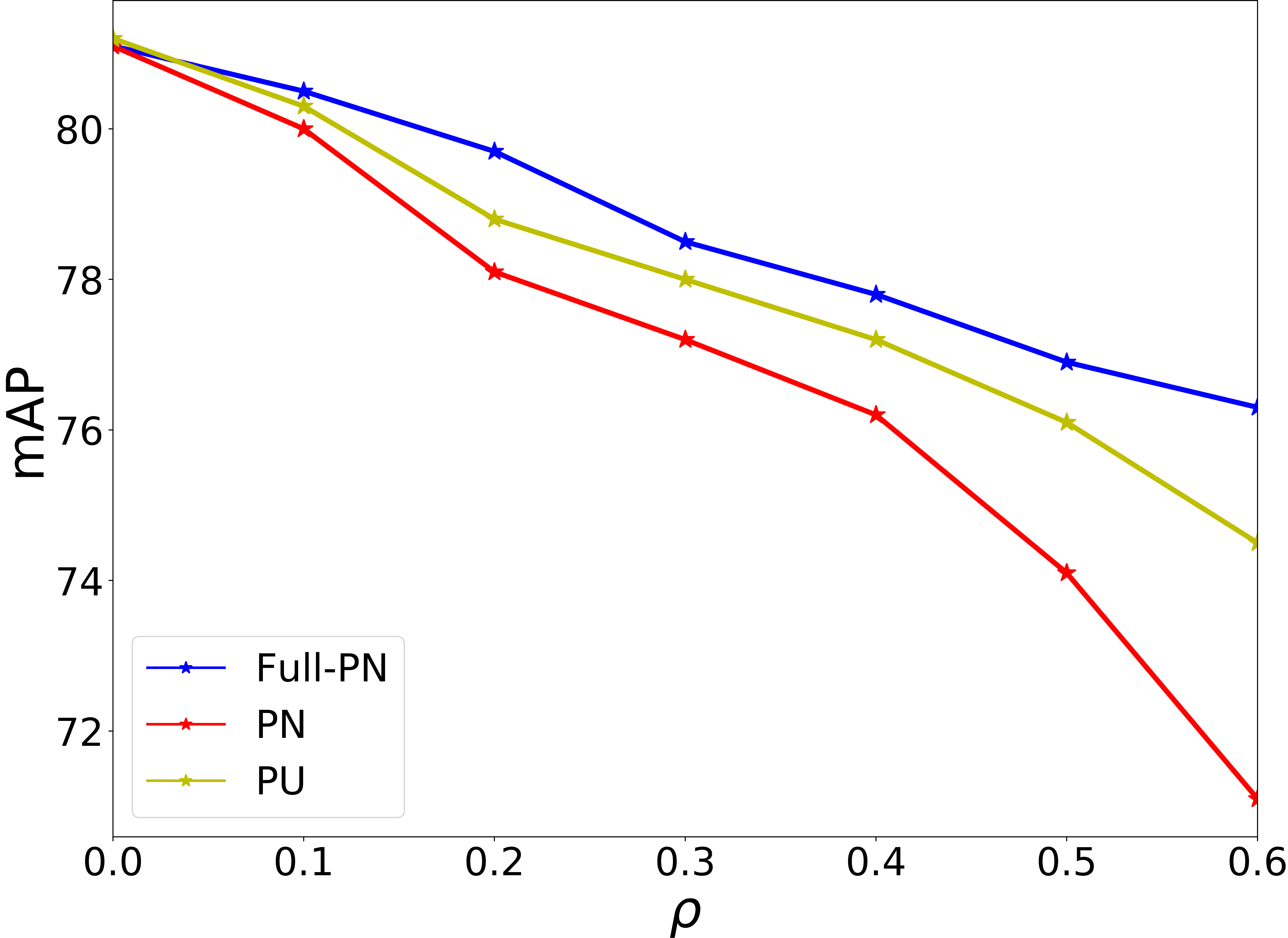
(a) PASCAL VOC

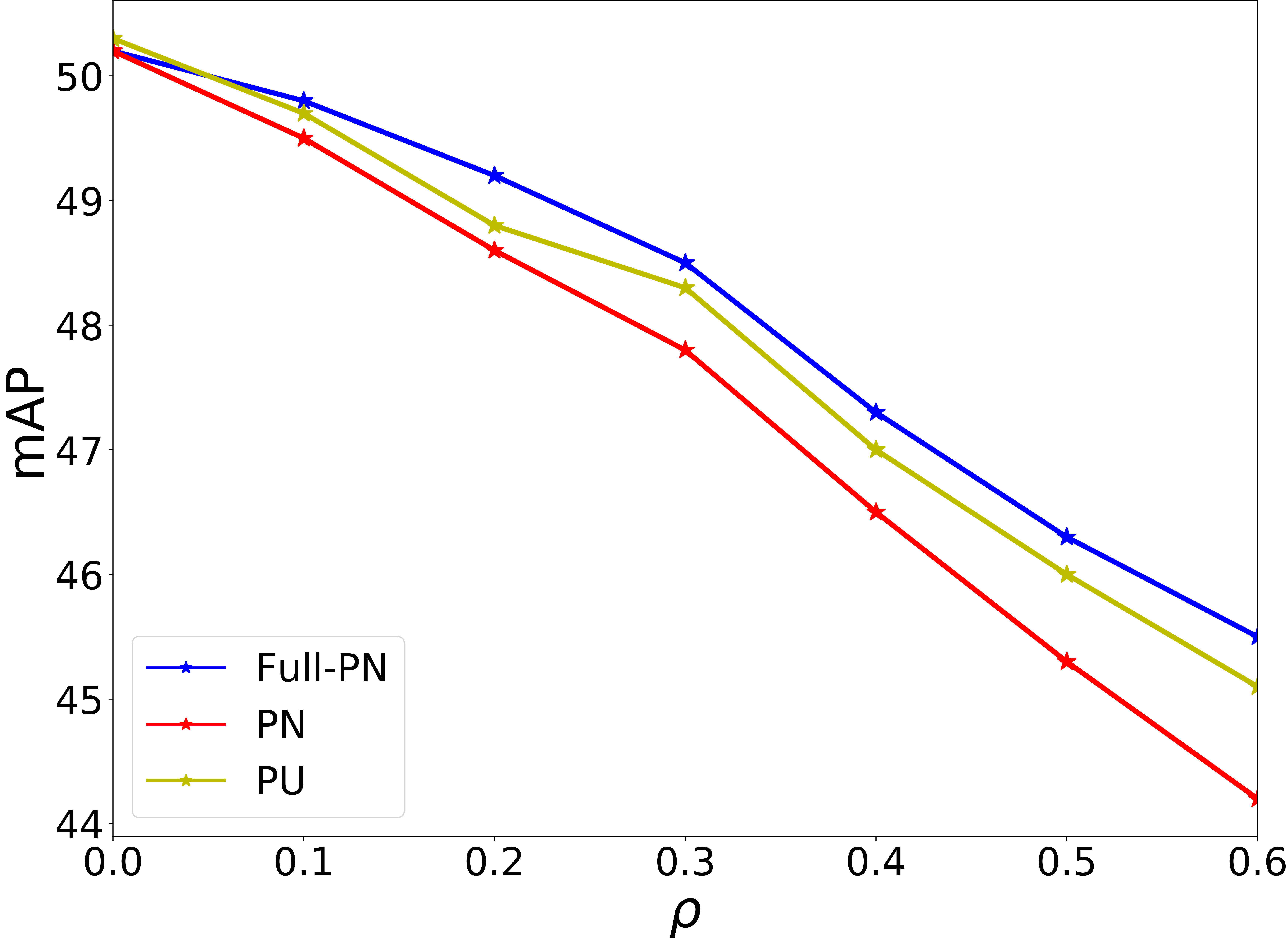
(b) MS COCO

Figure 5: mAP at IoU 0.5 ($\text{AP}_{50}$) on (a) PASCAL VOC and (b) MS COCO, for a range of label missingness $\rho$.

4.2 PU versus PN on PASCAL VOC and MS COCO

We investigate the effect that incomplete labels have on object detection training for the popular datasets PASCAL VOC [Everingham et al.(2010)Everingham, Van Gool, Williams, Winn, and Zisserman] and MS COCO [Lin et al.(2014)Lin, Maire, Belongie, Bourdev, Girshick, Hays, Perona, Ramanan, Zitnick, and Dolí], using Faster R-CNN [Ren et al.(2015)Ren, He, Girshick, and Sun] with a ResNet101 [He et al.(2016)He, Zhang, Ren, and Sun] convolutional feature extractor. In order to quantify the effect of missing labels, we artificially discard a proportion $\rho$ of the annotations. We compare three settings, each for a range of values of $\rho$. Given that the annotations are the source of the learning signal, we keep the number of total instances constant between settings for each $\rho$ as follows:

• PN: We remove a proportion of labels from every image in the dataset, such that the total proportion of removed labels is equal to $\rho$, and all images are included in the training set. We then train the detection model with a PN objective, as is normal.

• Full-PN: We discard a proportion $\rho$ of entire images and their labels, resulting in a dataset of fewer images, but each of which retains its complete annotations.

• PU: We use the same images and labels as in PN, but instead train with our proposed PU objective.

A comparison of mean average precision (mAP) performance at IoU 0.5 for these 3 settings on PASCAL VOC and MS COCO is shown in Figure 5. As expected, as $\rho$ is increased, the detector’s performance degrades. Focusing on the results for PN and Full-PN, it is clear that for an equal number of annotated objects, having fewer images that are more thoroughly annotated is preferable to a larger number of images with less thorough labels. On the other hand, considering object detection as a PU (PU) problem as we have proposed allows us to improve detector quality across a wide range of label missingness. While having a more carefully annotated set (Full-PN) is still superior, the PU objective helps close the gap. Interestingly, there is a small gain (PASCAL VOC: +0.2, MS COCO: +0.3) in mAP at full labels ($\rho=0$), possibly due to better learning of objects missing labels in the full dataset. Additional analysis on the improvements to RPN recall are in Supplemental Materials Section B.

4.3 Visual Genome

Table 1: Detector performance on Visual Genome, with full labels, at various IoU thresholds. “Y” indicates weighting by class frequency, while “N” denotes without weighting.

	$\text{AP}_{25}$		$\text{AP}_{50}$		$\text{AP}_{75}$
	Y	N	Y	N	Y	N
PN	12.09	22.79	9.11	17.35	2.46	9.98
PU	13.83	25.56	10.44	19.89	4.52	11.79

Visual Genome [Krishna et al.(2017)Krishna, Zhu, Groth, Johnson, Hata, Kravitz, Chen, Kalantidis, Li, Shamma, Bernstein, and Fei-Fei] is a scene understanding dataset of objects, attributes, and relationships. While not as commonly used as an object detection benchmark as PASCAL VOC or MS COCO, Visual Genome is popular when relationships or attributes of objects are desired, as when Faster R-CNN is used as a pre-trained feature extractor for Visual Question Answering [Agrawal et al.(2015)Agrawal, Lu, Antol, Mitchell, Zitnick, Batra, and Parikh, Anderson et al.(2018)Anderson, He, Buehler, Teney, Johnson, Gould, and Zhang]. Given the large number of classes (33,877) and the focus on scene understanding during the annotation process, the label coverage of all object instances present in each image is correspondingly lower. In order to achieve its scale, the labeling effort was crowd-sourced to a large number of human annotators. As pointed out in [Everingham et al.(2010)Everingham, Van Gool, Williams, Winn, and Zisserman], even increasing from 10 classes of objects in PASCAL VOC2006 to the 20 in VOC2007 resulted in a substantially larger number of labeling errors, as it became more difficult for human annotators to remember all of the object classes. This problem is worse by several orders of magnitude for Visual Genome. While the dataset creators implemented certain measures to ensure quality, there still are many examples of missing labels. In such a setting, the proposed PU risk estimation is especially appropriate, even with all included labels.

We train ResNet101 Faster R-CNN using both PN and the proposed PU risk estimation on 1600 of the top object classes of Visual Genome, as in [Anderson et al.(2018)Anderson, He, Buehler, Teney, Johnson, Gould, and Zhang]. We evaluate performance on the classes present in the test set and report mAP at various IoU thresholds $\{0.25,0.50,0.75\}$ in Table 1. We also show mAP results when each class’s average precision is weighted according to class frequency, as done in [Anderson et al.(2018)Anderson, He, Buehler, Teney, Johnson, Gould, and Zhang]. The PASCAL VOC and MS COCO results in Figure 5 indicate that we might expect increasing benefit from utilizing a PU loss as missing labels become especially prevalent, and for Visual Genome, where this is indeed the case, we observe that PU risk estimation outperforms PN by a significant margin, across all settings. Similar improvements are also observed on OpenImages [Krasin et al.(2016)Krasin, Duerig, Alldrin, Ferrari, Abu-El-Haija, Kuznetsova, Rom, Uijlings, Popov, Veit, Belongie, Gomes, Gupta, Sun, Chechik, Cai, Feng, Narayanan, and Murphy, Kuznetsova et al.(2018)Kuznetsova, Rom, Alldrin, Uijlings, Krasin, Pont-Tuset, Kamali, Popov, Malloci, Duerig, and Ferrari], a dataset with a similar degree of object missingness (Supplemental Materials Section C).

4.4 DeepLesion

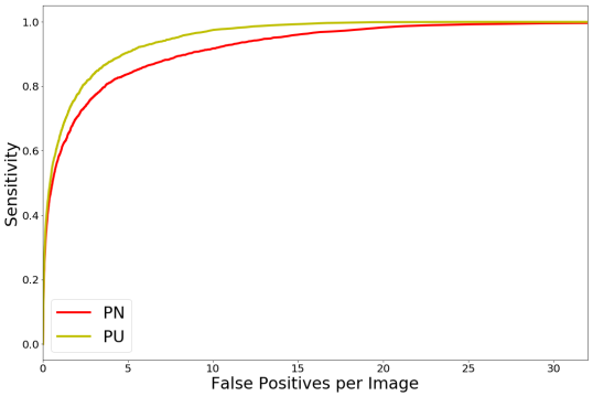
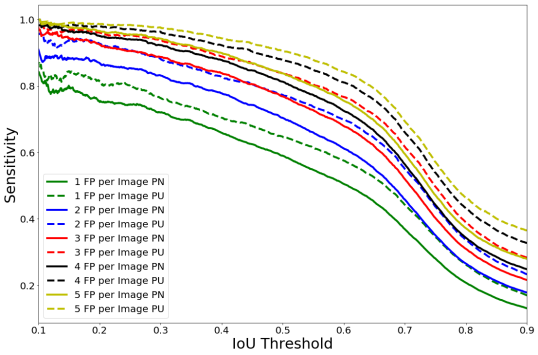
Figure 6: Lesion sensitivity versus (a) false positive rate and (b) IoU threshold for different false positive (FP) allowances per image. We compare the baseline Faster R-CNN variant in [Yan et al.(2017)Yan, Wang, Lu, and Summers] trained with a PN objective versus the proposed PU objective.

The recent progress in computer vision has attracted increasing attention towards potential health applications. To encourage deep learning research in this direction, the National Institutes of Health (NIH) Clinical Center released DeepLesion [Yan et al.(2017)Yan, Wang, Lu, and Summers], a dataset consisting of 32K CT scans with annotated lesions. Unlike PASCAL VOC, MS COCO, or Visual Genome, labeling cannot be crowd-sourced for most medical datasets, as accurate labeling requires medical expertise. Even with medical experts, labeling can be inconsistent; lesion detection is a challenging task, with biopsy often necessary to get an accurate result. Like other datasets labeled by an ensemble of annotators, the ground truth of medical datasets may contain inconsistencies, with some doctors being more conservative or aggressive in their diagnoses. Due to these considerations, a PU approach more accurately characterizes the nature of the data.

We re-implemented the modified version of Faster R-CNN described in [Yan et al.(2017)Yan, Wang, Lu, and Summers] as the baseline model and compare against our proposed model using the PU objective, making no other changes. We split the dataset into 70%-15%-15% parts for training, validation, and test. Following [Yan et al.(2017)Yan, Wang, Lu, and Summers], we report results in terms of free receiver operating characteristic (FROC) and sensitivity of lesion detection versus intersection-over-union (IoU) threshold for a range of allowed false positives (FP) per image (Figure 6). In both cases, we show that switching from a PN objective to a PU one results in gains in performance.

5 Conclusion and future work

Having observed that object detection data more closely resembles a positive-unlabeled (PU) problem, we propose training object detection models with a PU objective. Such an objective requires estimation of the class probability of the positive class, but we demonstrate how this can be estimated dynamically with little modification to the existing architecture. Making these changes allows us to achieve improved detection performance across a diverse set of datasets, some of which are real datasets with significant labeling difficulties. While we primarily focused our attention on object detection, a number of other popular tasks share similar characteristics and could also benefit from being recast as PU learning problems (e.g., segmentation [Ronneberger et al.(2015)Ronneberger, Fischer, and Brox, Long et al.(2015)Long, Shelhamer, and Darrell, He et al.(2017)He, Gkioxari, Dollár, and Girshick], action detection [Soomro et al.(2012)Soomro, Zamir, and Shah, Idrees et al.(2017)Idrees, Zamir, Jiang, Gorban, Laptev, Sukthankar, and Shah, Gu et al.(2018)Gu, Sun, Ross, Vondrick, Pantofaru, Li, Vijayanarasimhan, Toderici, Ricco, Sukthankar, Schmid, and Malik]).

In our current implementation, we primarily focus on applying the PU objective to the binary object-or-not classifier in Faster R-CNN’s Region Proposal Network. A natural extension of this work would be to apply the same objective to the second stage classifier, which must also separate objects from background. However, as the second stage classifier outputs one of several classes (or background), the classification is no longer binary, and requires estimating multiple class priors $\{\pi_{c}\}_{c=1}^{k}$ [Xu et al.(2017)Xu, Xu, Xu, and Tao], which we leave to future work. Such a multi-class PU loss would also allow extension to single-stage detectors like SSD [Liu et al.(2016)Liu, Anguelov, Erhan, Szegedy, Reed, Fu, and Berg] and YOLO [Redmon et al.(2016)Redmon, Divvala, Girshick, and Farhadi, Redmon and Farhadi(2017)]. Given the performance gains already observed, we believe this to be an effective and natural improvement to the object detection classification loss.

Appendix A Example forgetting in object detection

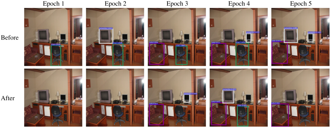
Figure 7: Detections on a PASCAL VOC train set image missing annotations throughout training: only the sofa in the lower left has a label. Each column shows detections directly before (top) and after (bottom) the model is trained on the image shown, for each epoch. While the sofa is consistently detected (purple box) after being learned, the unlabeled objects (2 monitors, a chair) are repeatedly found and then suppressed after being trained upon.

In a recent study of training dynamics of neural network classifiers, Toneva et al.(2019)Toneva, Sordoni, des Combes, Trischler, Bengio, and Gordon defined a “forgetting event” as a training example switching from being classified correctly by the model to being classified incorrectly during training. It was found that certain examples were forgotten more frequently than others while others were never forgotten (termed “unforgettable”), with the degree of forgetting for individual examples being consistent across neural network architectures and random seeds. When visualized, the forgotten examples tend to have atypical or uncommon characteristics (e.g., pose, lighting, angle), relative to “unforgettable” examples. Interestingly, a significant number of “unforgettable” examples could be removed from the training set with only a marginal reduction in test accuracy, if the “hard” examples were kept. This implies that the “hard” examples play a role akin to support vectors in max-margin learning, while easier “unforgettable” examples have little effect on the final decision boundary.

Within the context of object detection datasets, we hypothesize that unlabeled object instances form a similar group of hard examples that are also learned and then forgotten throughout training. Unlike the inter-batch catastrophic forgetting in Toneva et al.(2019)Toneva, Sordoni, des Combes, Trischler, Bengio, and Gordon, however, where hard examples are learned while part of the current minibatch and then forgotten while learning other examples, unlabeled samples in object detection are learned from other examples and then suppressed after incurring misclassification losses during training (see Figure 7).

Unlabeled instances strongly resemble positive examples throughout the rest of the dataset, but their lack of labels mean that the typical PN classification objective incentivizes learning them as negatives. Given that hard examples have a strong influence on classifier boundaries, having unlabeled examples trained as negatives may prove especially detrimental to training.

We perform a similar study as Toneva et al.(2019)Toneva, Sordoni, des Combes, Trischler, Bengio, and Gordon and investigate forgetting events on PASCAL VOC Everingham et al.(2010)Everingham, Van Gool, Williams, Winn, and Zisserman by tracking detection rates of labeled and unlabeled instances in the training set throughout learning. In particular, an object is considered detected if the detector produces a bounding box with intersection over union (IoU) of at least 0.5 and the classifier is at least 80% confident in the correct class. We track whether or not an object was detected directly before the image it belongs to is trained upon, and then again after the gradients have been applied. These indicator variables are then combined across objects for each epoch and reported as a percentage. While PASCAL VOC does naturally have unlabeled instances, we do not have access to these without a re-labeling effort. As such, we remove $10\%$ of object annotations randomly across all object classes during training, and use them to calculate detection rates for this experiment.

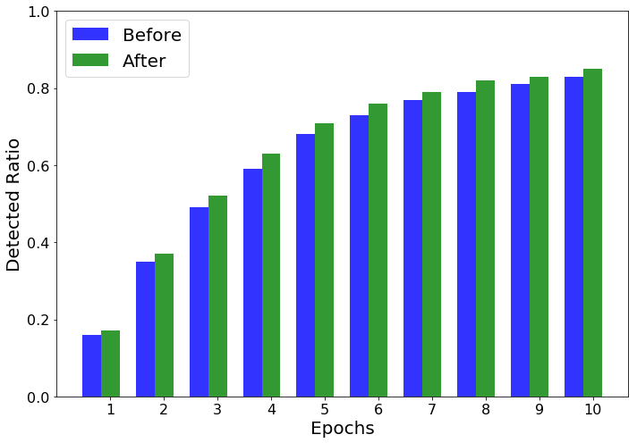
(a) Labeled objects

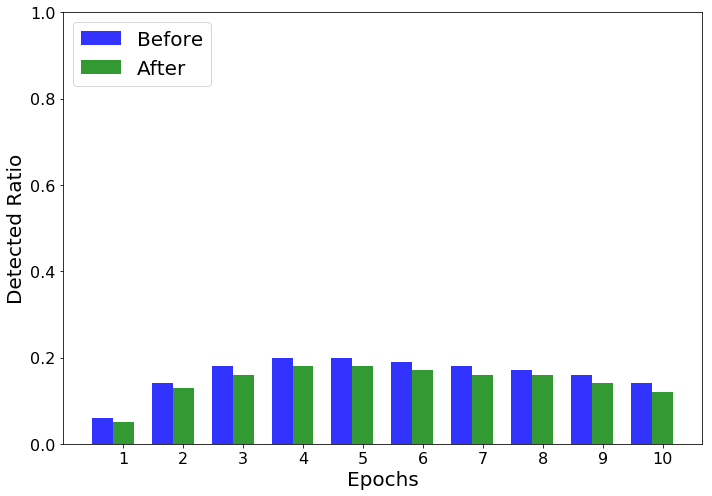
(b) Unlabeled objects

Figure 8: Detection rates of objects before and after training on their corresponding images for (a) labeled instances and (b) instances with labels withheld during training.

Detection rates for labeled and unlabeled objects over time are shown in Figure 8. As expected, the model learns to detect a higher percentage of labeled instances over time, and objects are overall more likely to be detected immediately after the detector trains on them. Despite not having an explicit learning signal, unlabeled objects are still learned throughout training, but at a lower rate than labeled ones. In contrast with labeled objects, unlabeled object detections are discouraged with each PN gradient, leading to a dip in overall detection rates immediately after training. Despite this, overall detection rates of unlabeled objects grows through the first 5 epochs of training, implying a repeated cycle of learning unlabeled objects from other intra-class examples, forgetting them when explicitly trained against them, and then learning them again. Given the undesirability of this forced suppression of detected objects, we seek a method to remedy this behavior.

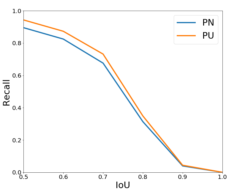
Figure 9: Recall of top 500 proposals from RPN after training on PASCAL VOC2007 when $\rho=0.5$.

Appendix B Recall of Region Proposals

To investigate the effect of the PU risk estimator on the quality of the proposals from RPN stage, we examine the recall of the top 500 proposals, compared with the complete annotations. Higher recall means there are more proposals that match with the full-labeled annotations. In Figure 9, the recalls using the PU risk estimator are higher than those using the PN risk estimator. This illustrates the inclusion of more object proposals that are not included by the PN risk estimator because the corresponding ground truth annotations are missing.

Appendix C OpenImages

OpenImages Krasin et al.(2016)Krasin, Duerig, Alldrin, Ferrari, Abu-El-Haija, Kuznetsova, Rom, Uijlings, Popov, Veit, Belongie, Gomes, Gupta, Sun, Chechik, Cai, Feng, Narayanan, and Murphy; Kuznetsova et al.(2018)Kuznetsova, Rom, Alldrin, Uijlings, Krasin, Pont-Tuset, Kamali, Popov, Malloci, Duerig, and Ferrari is a large object dataset consisting of 15.4 million bounding boxes from 600 classes across 1.9 million images. In order to achieve its scale, the labeling effort was crowd-sourced to a large number of human annotators. As pointed out in Everingham et al.(2010)Everingham, Van Gool, Williams, Winn, and Zisserman, even increasing from 10 classes of objects in PASCAL VOC2006 to the 20 in VOC2007 resulted in a substantially larger number of labeling errors, as it became more difficult for human annotators to remember all of the object classes. With 500 classes, this problem is worse by an order of magnitude for OpenImages. While the creators of OpenImages designed an annotator training process to insure quality, there still are many examples of missing labels. As such, PU learning as proposed is especially appropriate, even when considering full labels.

As in Section 4.2, we train a ResNet101 Faster R-CNN object detector with both PN and PU classification losses. Given the large size of the dataset, we restrict our analysis to 50 of the most prevalent classes, and subsample 140K images from the dataset containing at least one of the selected classes. Of these 140K images, we train on 100K with full annotations, and hold out 10K for validation and 30K as our test split. We observe that, all other things equal, switching to our proposed PU approach results in an increase of $+3.0$, $+3.0$, and $+5.0$ for mAPs with IoU thresholds $\{0.25,0.50,0.75\}$ (see Table 2).

Table 2: Detector performance on a subset of OpenImages at various IoU thresholds.

Method	$\text{AP}_{25}$	$\text{AP}_{50}$	$\text{AP}_{75}$
PN	37.7	33.6	20.7
PU	40.7	36.6	25.7

References

- [Agrawal et al.(2015)Agrawal, Lu, Antol, Mitchell, Zitnick, Batra, and Parikh] Aishwarya Agrawal, Jiasen Lu, Stanislaw Antol, Margaret Mitchell, C. Lawrence Zitnick, Dhruv Batra, and Devi Parikh. VQA: Visual Question Answering. International Conference on Computer Vision, 2015.
- [Anderson et al.(2018)Anderson, He, Buehler, Teney, Johnson, Gould, and Zhang] Peter Anderson, Xiaodong He, Chris Buehler, Damien Teney, Mark Johnson, Stephen Gould, and Lei Zhang. Bottom-Up and Top-Down Attention for Image Captioning and Visual Question Answering. Conference on Computer Vision and Pattern Recognition, 2018.
- [Bilen and Vedaldi(2016)] Hakan Bilen and Andrea Vedaldi. Weakly Supervised Deep Detection Networks. Conference on Computer Vision and Pattern Recognition, 2016.
- [Dai et al.(2016)Dai, Li, He, and Sun] Jifeng Dai, Yi Li, Kaiming He, and Jian Sun. R-FCN: Object Detection via Region-based Fully Convolutional Networks. Advances In Neural Information Processing Systems, 2016.
- [De Comité et al.(1999)De Comité, Denis, Gilleron, and Letouzey] Francesco De Comité, François Denis, Rémi Gilleron, and Fabien Letouzey. Positive and Unlabeled Examples Help Learning. Algorithmic Learning Theory, 1999.
- [Deng et al.(2009)Deng, Dong, Socher, Li, Li, and Li] Jia Deng, Wei Dong, Richard Socher, Li-Jia Li, Kai Li, and Fei-Fei Li. ImageNet: A large-scale hierarchical image database. Conference on Computer Vision and Pattern Recognition, 2009.
- [Denis(1998)] François Denis. PAC Learning from Positive Statistical Queries. Algorithmic Learning Theory, 1998.
- [Dong et al.(2018)Dong, Zheng, Ma, Yang, and Meng] Xuanyi Dong, Liang Zheng, Fan Ma, Yi Yang, and Deyu Meng. Few-shot Object Detection. Transactions on Pattern Analysis and Machine Intelligence, 2018.
- [Du Plessis et al.(2015)Du Plessis, Niu, and Sugiyama] Marthinus Du Plessis, Gang Niu, and Masashi Sugiyama. Convex formulation for learning from positive and unlabeled data. In International Conference on Machine Learning, pages 1386–1394, 2015.
- [Du Plessis et al.(2014)Du Plessis, Niu, and Sugiyama] Marthinus C Du Plessis, Gang Niu, and Masashi Sugiyama. Analysis of learning from positive and unlabeled data. In Advances in neural information processing systems, pages 703–711, 2014.
- [Elkan and Noto(2008)] Charles Elkan and Keith Noto. Learning Classifiers from Only Positive and Unlabeled Data. International Conference on Knowledge Discovery and Data Mining, 2008.
- [Everingham et al.(2010)Everingham, Van Gool, Williams, Winn, and Zisserman] Mark Everingham, Luc Van Gool, Christopher K.I. Williams, John Winn, and Andrew Zisserman. The Pascal Visual Object Classes (VOC) Challenge. International Journal of Computer Vision, 2010. 10.1007/s11263-009-0275-4.
- [Girshick(2015)] Ross Girshick. Fast R-CNN. International Conference on Computer Vision, 2015.
- [Girshick et al.(2014)Girshick, Donahue, Darrell, and Malik] Ross Girshick, Jeff Donahue, Trevor Darrell, and Jitendra Malik. Rich feature hierarchies for accurate object detection and semantic segmentation. Conference on Computer Vision and Pattern Recognition, 2014.
- [Gu et al.(2018)Gu, Sun, Ross, Vondrick, Pantofaru, Li, Vijayanarasimhan, Toderici, Ricco, Sukthankar, Schmid, and Malik] Chunhui Gu, Chen Sun, David A. Ross, Carl Vondrick, Caroline Pantofaru, Yeqing Li, Sudheendra Vijayanarasimhan, George Toderici, Susanna Ricco, Rahul Sukthankar, Cordelia Schmid, and Jitendra Malik. AVA: A Video Dataset of Spatio-Temporally Localized Atomic Visual Actions. Conference on Computer Vision and Pattern Recognition, 2018.
- [He et al.(2016)He, Zhang, Ren, and Sun] Kaiming He, Xiangyu Zhang, Shaoqing Ren, and Jian Sun. Deep Residual Learning for Image Recognition. Conference on Computer Vision and Pattern Recognition, 2016.
- [He et al.(2017)He, Gkioxari, Dollár, and Girshick] Kaiming He, Georgia Gkioxari, Piotr Dollár, and Ross B. Girshick. Mask R-CNN. International Conference on Computer Vision, 2017.
- [Hoffman et al.(2014)Hoffman, Guadarrama, Tzeng, Donahue, Girshick, Darrell, and Saenko] Judy Hoffman, Sergio Guadarrama, Eric Tzeng, Jeff Donahue, Ross B. Girshick, Trevor Darrell, and Kate Saenko. LSDA: Large Scale Detection Through Adaptation. Advances In Neural Information Processing Systems, 2014.
- [Idrees et al.(2017)Idrees, Zamir, Jiang, Gorban, Laptev, Sukthankar, and Shah] Haroon Idrees, Amir R. Zamir, Yu-Gang Jiang, Alex Gorban, Ivan Laptev, Rahul Sukthankar, and Mubarak Shah. The THUMOS challenge on action recognition for videos “in the wild”. Computer Vision and Image Understanding, 2017.
- [Jain et al.(2016)Jain, White, and Radivojac] Shantanu Jain, Martha White, and Predrag Radivojac. Estimating the class prior and posterior from noisy positives and unlabeled data. In Advances in neural information processing systems, pages 2693–2701, 2016.
- [Jiang et al.(2018)Jiang, Zhou, Leung, Li, and Fei-Fei] Lu Jiang, Zhengyuan Zhou, Thomas Leung, Li-Jia Li, and Li Fei-Fei. MentorNet: Learning Data-Driven Curriculum for Very Deep Neural Networks on Corrupted Labels. International Conference on Machine Learning, 2018.
- [Kiryo et al.(2017)Kiryo, Niu, Du Plessis, and Sugiyama] Ryuichi Kiryo, Gang Niu, Marthinus C Du Plessis, and Masashi Sugiyama. Positive-Unlabeled Learning with Non-Negative Risk Estimator. Advances In Neural Information Processing Systems, 2017.
- [Krasin et al.(2016)Krasin, Duerig, Alldrin, Ferrari, Abu-El-Haija, Kuznetsova, Rom, Uijlings, Popov, Veit, Belongie, Gomes, Gupta, Sun, Chechik, Cai, Feng, Narayanan, and Murphy] Ivan Krasin, Tom Duerig, Neil Alldrin, Vittorio Ferrari, Sami Abu-El-Haija, Alina Kuznetsova, Hassan Rom, Jasper Uijlings, Stefan Popov, Andreas Veit, Serge Belongie, Victor Gomes, Abhinav Gupta, Chen Sun, Gal Chechik, David Cai, Zheyun Feng, Dhyanesh Narayanan, and Kevin Murphy. OpenImages: A public dataset for large-scale multi-label and multi-class image classification. Dataset available from https://github.com/openimages, 2016.
- [Krishna et al.(2017)Krishna, Zhu, Groth, Johnson, Hata, Kravitz, Chen, Kalantidis, Li, Shamma, Bernstein, and Fei-Fei] Ranjay Krishna, Yuke Zhu, Oliver Groth, Justin Johnson, Kenji Hata, Joshua Kravitz, Stephanie Chen, Yannis Kalantidis, Li-Jia Li, David A. Shamma, Michael S. Bernstein, and Li Fei-Fei. Visual Genome: Connecting Language and Vision Using Crowdsourced Dense Image Annotations. International Journal Computer Vision, 2017.
- [Krizhevsky et al.(2012)Krizhevsky, Sutskever, and Hinton] Alex Krizhevsky, Ilya Sutskever, and Geoffrey E Hinton. ImageNet Classification with Deep Convolutional Neural Networks. Advances In Neural Information Processing Systems, 2012.
- [Kuznetsova et al.(2018)Kuznetsova, Rom, Alldrin, Uijlings, Krasin, Pont-Tuset, Kamali, Popov, Malloci, Duerig, and Ferrari] Alina Kuznetsova, Hassan Rom, Neil Alldrin, Jasper Uijlings, Ivan Krasin, Jordi Pont-Tuset, Shahab Kamali, Stefan Popov, Matteo Malloci, Tom Duerig, and Vittorio Ferrari. The Open Images Dataset V4: Unified image classification, object detection, and visual relationship detection at scale. arXiv preprint, 2018.
- [Lecun et al.(1989)Lecun, Boser, Denker, Henderson, Howard, Hubbard, and Jackel] Y. Lecun, B. Boser, J.S Denker, D. Henderson, R. E. Howard, W. Hubbard, and L. D. Jackel. Backpropagation Applied to Handwritten Zip Code Recognition. Neural Computation, 1989.
- [Lee et al.(2017)Lee, Gimenez, Hoogi, Miyake, Gorovoy, and Rubin] Rebecca Sawyer Lee, Francisco Gimenez, Assaf Hoogi, Kanae Kawai Miyake, Mia Gorovoy, and Daniel L. Rubin. A curated mammography data set for use in computer-aided detection and diagnosis research. Nature Scientific Data, 2017.
- [Lee and Liu(2003)] Wee Sun Lee and Bing Liu. Learning with positive and unlabeled examples using weighted logistic regression. In ICML, volume 3, pages 448–455, 2003.
- [Letouzey et al.(2000)Letouzey, Denis, and Gilleron] Fabien Letouzey, François Denis, and Rémi Gilleron. Learning from Positive and Unlabeled Examples. Algorithmic Learning Theory, 2000.
- [Liang et al.(2018)Liang, Heilmann, Gregory, Diallo, Carlson, Spell, Sigman, Roe, and Carin] Kevin J Liang, Geert Heilmann, Christopher Gregory, Souleymane O. Diallo, David Carlson, Gregory P. Spell, John B. Sigman, Kris Roe, and Lawrence Carin. Automatic Threat Recognition of Prohibited Items at Aviation Checkpoint with X-ray Imaging: A Deep Learning Approach. SPIE Anomaly Detection and Imaging with X-Rays (ADIX) III, 2018.
- [Lin et al.(2014)Lin, Maire, Belongie, Bourdev, Girshick, Hays, Perona, Ramanan, Zitnick, and Dolí] Tsung-Yi Lin, Michael Maire, Serge Belongie, Lubomir Bourdev, Ross Girshick, James Hays, Pietro Perona, Deva Ramanan, C Lawrence Zitnick, and Piotr Dolí. Microsoft COCO: Common Objects in Context. European Conference on Computer Vision, 2014.
- [Lin et al.(2017)Lin, Dollár, Girshick, He, Hariharan, and Belongie] Tsung-Yi Lin, Piotr Dollár, Ross Girshick, Kaiming He, Bharath Hariharan, and Serge Belongie. Feature Pyramid Networks for Object Detection. Computer Vision and Pattern Recognition, pages 2117–2125, 2017.
- [Liu et al.(2016)Liu, Anguelov, Erhan, Szegedy, Reed, Fu, and Berg] Wei Liu, Dragomir Anguelov, Dumitru Erhan, Christian Szegedy, Scott Reed, Cheng-Yang Fu, and Alexander C Berg. SSD: Single Shot MultiBox Detector. European Conference on Computer Vision, 2016.
- [Long et al.(2015)Long, Shelhamer, and Darrell] Jonathan Long, Evan Shelhamer, and Trevor Darrell. Fully Convolutional Networks for Semantic Segmentation. Conference on Computer Vision and Pattern Recognition, 2015.
- [Moreira et al.(2012)Moreira, Amaral, Domingues, Cardoso, Cardoso, and Cardoso] Inês C. Moreira, Igor Amaral, Inês Domingues, Antó́nio Cardoso, Maria Joã̃o Cardoso, and Jaime S. Cardoso. INbreast: Toward a Full-field Digital Mammographic Database. Academic Radiology, 2012.
- [Oquab et al.(2015)Oquab, Bottou, Laptev, and Sivic] Maxime Oquab, Léon Bottou, Ivan Laptev, and Josef Sivic. Is object localization for free? Weakly-supervised learning with convolutional neural networks. Conference on Computer Vision and Pattern Recognition, 2015.
- [Rame et al.(2018)Rame, Garreau, Ben-Younes, and Ollion] Alexandre Rame, Emilien Garreau, Hedi Ben-Younes, and Charles Ollion. OMNIA Faster R-CNN: Detection in the wild through dataset merging and soft distillation. arXiv preprint, 2018.
- [Redmon and Farhadi(2017)] Joseph Redmon and Ali Farhadi. YOLO9000: Better, Faster, Stronger. Conference on Computer Vision and Pattern Recognition, 2017.
- [Redmon et al.(2016)Redmon, Divvala, Girshick, and Farhadi] Joseph Redmon, Santosh Divvala, Ross Girshick, and Ali Farhadi. You Only Look Once: Unified, Real-Time Object Detection. Conference on Computer Vision and Pattern Recognition, 2016.
- [Ren et al.(2015)Ren, He, Girshick, and Sun] Shaoqing Ren, Kaiming He, Ross Girshick, and Jian Sun. Faster R-CNN: Towards Real-Time Object Detection with Region Proposal Networks. Advances in Neural Information Processing Systems, 2015.
- [Rochan and Wang(2015)] Mrigank Rochan and Yang Wang. Weakly supervised localization of novel objects using appearance transfer. Conference on Computer Vision and Pattern Recognition, 2015.
- [Ronneberger et al.(2015)Ronneberger, Fischer, and Brox] Olaf Ronneberger, Philipp Fischer, and Thomas Brox. U-Net: Convolutional Networks for Biomedical Image Segmentation. Medical Image Computing and Computer Assisted Intervention, 2015.
- [Sigman et al.(2020)Sigman, Spell, Liang, and Carin] John B. Sigman, Gregory P. Spell, Kevin J Liang, and Lawrence Carin. Background Adaptive Faster R-CNN for Semi-supervised Convolutional Object Detection of Threats in X-ray Images. SPIE Anomaly Detection and Imaging with X-Rays (ADIX) V, 2020.
- [Soomro et al.(2012)Soomro, Zamir, and Shah] Khurram Soomro, Amir Roshan Zamir, and Mubarak Shah. UCF101: A dataset of 101 human actions classes from videos in the wild. T. Technical Report CRCV-TR-12-01, University of Central Florida, 2012.
- [Tang et al.(2016)Tang, Wang, Gao, Dellandrea, Gaizauskas, and Chen] Yuxing Tang, Josiah Wang, Boyang Gao, Emmanuel Dellandrea, Robert Gaizauskas, and Liming Chen. Large Scale Semi-Supervised Object Detection Using Visual and Semantic Knowledge Transfer. Conference on Computer Vision and Pattern Recognition, 2016.
- [Toneva et al.(2019)Toneva, Sordoni, des Combes, Trischler, Bengio, and Gordon] Mariya Toneva, Alessandro Sordoni, Remi Tachet des Combes, Adam Trischler, Yoshua Bengio, and Geoffrey J. Gordon. An Empirical Study of Example Forgetting during Deep Neural Network Learning. International Conference on Learning Representations, 2019.
- [Veit et al.(2017)Veit, Alldrin, Chechik, Krasin, Gupta, and Belongie] Andreas Veit, Neil Alldrin, Gal Chechik, Ivan Krasin, Abhinav Gupta, and Serge Belongie. Learning From Noisy Large-Scale Datasets With Minimal Supervision. Conference on Computer Vision and Pattern Recognition, 2017.
- [Wang et al.(2017)Wang, Peng, Lu, Lu, Bagheri, and Summers] Xiaosong Wang, Yifan Peng, Le Lu, Zhiyong Lu, Mohammadhadi Bagheri, and Ronald M. Summers. ChestX-ray8: Hospital-Scale Chest X-Ray Database and Benchmarks on Weakly-Supervised Classification and Localization of Common Thorax Diseases. Conference on Computer Vision and Pattern Recognition, 2017.
- [Wu et al.(2019)Wu, Bodla, Singh, Najibi, Chellappa, and Davis] Zhe Wu, Navaneeth Bodla, Bharat Singh, Mahyar Najibi, Rama Chellappa, and Larry S. Davis. Soft Sampling for Robust Object Detection. British Machine Vision Conference, 2019.
- [Xu et al.(2017)Xu, Xu, Xu, and Tao] Yixing Xu, Chang Xu, Chao Xu, and Dacheng Tao. Multi-positive and unlabeled learning. In IJCAI, pages 3182–3188, 2017.
- [Yan et al.(2017)Yan, Wang, Lu, and Summers] Ke Yan, Xiaosong Wang, Le Lu, and Ronald M. Summers. DeepLesion: Automated Deep Mining, Categorization and Detection of Significant Radiology Image Findings using Large-Scale Clinical Lesion Annotations. arXiv preprint, 2017.
- [Zhang et al.(2017)Zhang, Bengio, Brain, Hardt, Recht, Vinyals, and Deepmind] Chiyuan Zhang, Samy Bengio, Google Brain, Moritz Hardt, Benjamin Recht, Oriol Vinyals, and Google Deepmind. Understanding Deep Learning Requires Re-thinking Generalization. International Conference on Learning Representations, 2017.