Some remarks on equilateral triangulations of surfaces and Belyi functions

Abstract.

In this paper, following Grothendieck Esquisse d’un programme, which was motivated by Belyi’s work, we study some properties of surfaces $X$ which are triangulated by (possibly ideal) isometric equilateral triangles of one of the spherical, euclidean or hyperbolic geometries. These surfaces have a natural Riemannian metric with conic singularities. In the euclidean case we analyze the closed geodesics and their lengths. Such surfaces can be given the structure of a Riemann surface which, considered as algebraic curves, are defined over $\bar{\mathbb{Q}}$ by a theorem of Belyi. They have been studied by many authors of course. Here we define the notion of connected sum of two Belyi functions and give some concrete examples. In the particular case when $X$ is a torus, the triangulation leads to an elliptic curve and we define the notion of a “peel” obtained from the triangulation (which is a metaphor of an orange peel) and relate this peel with the modulus $\tau$ of the elliptic curve. Many fascinating questions arise regarding the modularity of the elliptic curve and the geometric aspects of the Taniyama-Shimura-Weil theory.

Keywords. Belyi functions, arithmetic surfaces, triangulated surfaces

MSC2020 Classification. 14H57, 11G32, 11G99, 14H25, 30F45

1. Introduction

One beautiful and fundamental result of the second half of the XX century is the result by Belyi which characterizes complex Riemann surfaces which, regarded as algebraic curves, can be given by equations with coefficients in $\bar{\mathbb{Q}}$. Belyi’s theorem states: a Riemann surface $\Sigma$ is defined over $\bar{\mathbb{Q}}$ if and only if it admits a meromorphic function $f:\Sigma\to\hat{\mathbb{C}}=\mathbb{P}^{1}_{\mathbb{C}}$ (the Riemann sphere), with at most three critical values which can be taken, without loss of generality, to be $0$ $1$ and $\infty$.

This theorem fascinated Alexander Grothendieck for its simplicity and depth to a degree that it changed his line of investigation and wrote the epoch making paper Esquisse d’un Programme [Esquisse].

The function $f$ is called “a Belyi map” and topologically expresses $\Sigma$ as a branched cover over the Riemann sphere $\hat{\mathbb{C}}$ with branching points a subset of $\{0,1,\infty\}$ (if f has only two critical values then, $f$ is up to a change of coordinates, the function $f(z)=z^{n}$, for some $n>1$). Such a branched covering is completely determined by the inverse image $f^{-1}([0,1]):=\mathcal{D}_{f}$. Then $\mathcal{D}_{f}$ is a bipartite graph with colored vertices: “white” for the points in $f^{-1}(\{0\})$ and “black” for the points in $f^{-1}(\{1\})$. The graph $\mathcal{D}_{f}$ was named by Grothendieck himself Dessin d’enfant [Esquisse], but in this paper some times just name it dessin. Besides, $\Sigma\setminus\mathcal{D}_{f}$ is a union of open sets homeomorphic to the open unit disk. This endows $\Sigma$ with a decorated (cartographic) map. Reciprocally, given a compact, oriented, connected, smooth surface $\Sigma$ with a cartographic map $\mathcal{G}$ (i.e, an embedded graph) one can endow $\Sigma$ with a unique complex structure and a holomorphic map $f:\Sigma\to\overline{\mathbb{C}}=P^{1}_{\mathbb{C}}$ with critical values $0$ $1$ and $\infty$, such that $\mathcal{D}_{f}$ is $\mathcal{G}$. Voevodsky and Shabat in [VSh89] have shown that if a closed, connected surface has a triangulation by euclidean equilateral triangles, then the flat structure with conic singularities gives the surface the structure of Riemann surface which as an algebraic complex curve can be defined over $\bar{\mathbb{Q}}$. The same is true if the surface is triangulated with congruent hyperbolic triangles of angles $\frac{\pi}{p},\frac{\pi}{q},\frac{\pi}{r}$ ($p,q,r\in\mathbb{N},\,\,\frac{1}{p}+\frac{1}{q}+\frac{1}{r}<1$), including $p=q=r=\infty$ [CoItzWo94]: such surfaces are defined also over $\bar{\mathbb{Q}}$. The aim of this paper is to study some properties and constructions of decorated triangulated surfaces.

In this paper we have tried to follow the simplicity of the ideas that fascinated Grothendieck in the spirit of the expository paper [Gui14] and make self-contained.

2. Equilateral structures on surfaces

2.1. Canonical equilateral triangulation of the Riemann sphere.

Let us consider the equilateral euclidean triangle $\Delta$ with vertices $0,1,\omega$, where $\omega=\text{e}^{\frac{2i\pi}{6}}$ is the sixth primitive root of unity. Denote by $\bar{\Delta}$ the triangle which is the reflection of $\Delta$ with respect to the real axis (see Figure (1)). If we identify the boundaries of $\Delta$ and $\bar{\Delta}$ by means of the conjugation map $z\mapsto\bar{z}$, we obtain a compact surface of genus 0 with a triangulation by two triangles. Such a surface, homeomorphic to the sphere, has a natural complex structure which, in the complement of the vertices, is given by complex charts with changes of coordinates given by orientation-preserving euclidean isometries. In this paper $2\Delta$ will always denote this surface.

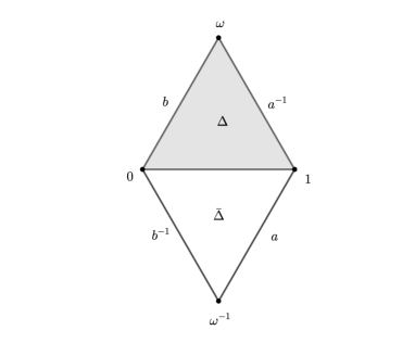
Figure 1. The sphere as the union of two equilateral triangles.

By the uniformization theorem (or Riemann-Roch’s theorem) any Riemann surface of genus 0 is conformally equivalent to the Riemann sphere. In fact, the Riemann surface $2\Delta$ defined in the previous paragraph can be uniformized explicitly as follows: consider the Schwarz-Christoffel map $\varphi\colon\bar{\mathbb{H}}\to\Delta$ defined by the formula

(1) $$\varphi(z)=C\int_{0}^{\zeta}\frac{dw}{w^{2/3}(w-1)^{2/3}},$$

where $C$ is an appropriate complex constant. The function $\varphi$ is a homeomorphism which maps conformally the upper half-plane $\mathbb{H}$ onto the interior of $\Delta$, and maps the points $0,1,\infty$ to $0,1,\omega$, respectively.

Let $\Omega$ be the region on $\mathbb{H}^{+}\cup\mathbb{H}^{-}\cup[0,1]$, and define the map $\Phi\colon\Omega\to\operatorname{Int}(\Delta\cup\bar{\Delta})$ as follows

(2) $$\Phi(z)=\begin{cases}\varphi(z),\ z\in\mathbb{H}^{+}\cup[0,1],\\ \overline{\varphi(\bar{z})},\ z\in\mathbb{H}^{-}\cup[0,1].\end{cases}$$

Schwarz reflection principle implies that $\Phi$ is conformal in $\Omega$. In addition, $\Phi$ induces a homeomorphism from the Riemann sphere $\hat{\mathbb{C}}$ to the quotient space. Abusing the notation we denote this function also by $\Phi$.

Applying Schwarz reflection principle to $\Phi$ in local coordinates we can verify that $\Phi$ is holomorphic in $\hat{\mathbb{C}}-\{0,1,\infty\}$. By Riemann extension theorem this map extends to the entire Riemann sphere.

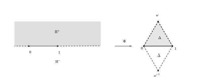
Figure 2. Schwarz-Christoffel map and its reflection.

Remark 1.

The flat metrics of the triangles $\Delta$ and $\bar{\Delta}$ induce a singular flat metric on $2\Delta$ and the two triangles form an equilateral triangulation of such surface. The vertices become conic singularities. Hence we can pull-back, via $\Phi$, this flat singular Riemannian metric to $\hat{\mathbb{C}}-\{0,1,\infty\}$. With this metric the upper and lower half-planes with marked points $0,1,\infty$ are isometric to equilateral euclidean triangles.

2.2. Equilateral euclidean triangulations on surfaces.

Definition 1.

(Euclidean triangulation) Let $X$ be a compact oriented surface. Then, a euclidean triangulation of $X$ is given by a set of homeomorphisms $\varphi_{i}\colon\Delta_{i}\to T_{i}$, where $\Delta_{i}$ are euclidean triangles with the additional condition that if $T_{i}$ and $T_{j}$ share an edge $a$, then the metrics on $a$ induced by $\varphi_{i}$ and $\varphi_{j}$ coincide. If all the triangles $\Delta_{i}$ are equilateral the triangulation is called equilateral triangulation.

Euclidean (respectively equilateral) triangulations on a surface will be also be referred as euclidean (respectively equilateral) triangulated structure on the surface.

Remark 2.

We don’t assume that the triangles of our triangulations meet at most in one common edge, we allow the triangles to meet in more than one edge.

Remark 3.

(a) If $a$ is a common edge of $T_{i}$ and $T_{j}$, then $\varphi_{i}\colon\Delta_{i}\to T_{i}$ and $\varphi_{j}\colon\Delta_{j}\to T_{j}$ induce the same linear metric on $a$ if and only if $\varphi_{i}^{-1}(a)$ and $\varphi_{j}^{-1}(a)$ have the same length and the barycentric coordinates in $a$, induced by $\varphi_{i}$ and $\varphi_{j}$, are the same.

(b) In an equilateral triangulation all the edges have the same length.

A triangulation of a surface $X$ with normal barycentric coordinates which is coherently oriented has a canonical complex structure. The charts around points which are not vertices are given as follows:

• Interior points. Let $\psi_{i}$ denote the inverse of the homeomorphism $\varphi_{i}:\Delta_{i}\to T_{i}$, then the map $\psi_{i}\colon\operatorname{Int}T_{i}\to\operatorname{Int}\Delta_{i}$ is a chart for all points in the interior of $T_{i}$.

• Points on the edges. Suppose that $a$ is a common edge of triangles the $T_{i}$ and $T_{j}$, let $R$ be the reflection with respect to the edge $\psi_{i}(a)$. There exists an orientation-preserving euclidean isometry $\mu_{j}$, which send $\Delta_{j}$ onto $R(\Delta_{i})$ and such that $\mu_{j}\circ\psi_{j}=\mu_{i}$ in $a$ (see Figure (3)).

  Define the homeomorphism $\Psi\colon T_{i}\cup T_{j}\to\Delta_{i}\cup R(\Delta_{i})$ as follows

  $$\Psi(x)=\begin{cases}\psi_{i}(x),\quad x\in T_{i}\\ \mu_{j}\circ\psi_{j}(x),\quad x\in T_{j}.\end{cases}$$

  Then we can choose as a chart for the points in the interior of the edge $a$ the previous map restricted to $\operatorname{Int}(T_{i}\cup T_{j})$. One can verify that this map is compatible with the charts defined in (i).

  

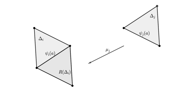
  Figure 3. The Isometry $\mu_{j}$.

One can show (see, for instance, [Spr81, Troy07]) that the complex structure extends to the vertices.

Since a euclidean triangulated structure on a surface is given by normal barycentric coordinates with a coherent orientation we have the following proposition:

Proposition 1.

A euclidean triangulated structure on $X$ induces a complex structure on $X$ which turns it into a Riemann surface and therefore (by Riemann) is an algebraic complex curve.

Remark 4.

The complex structure does not change if we rescale the euclidean triangles, so we may assume in all that follows that the edges have length one.

2.3. Belyi functions

Let $X$ be a compact Riemann surface. A meromorphic function $f\colon X\to\hat{\mathbb{C}}$ with critical values contained in the set $\{0,1,\infty\}$ will be called a Belyi function. If a compact Riemann surface $X$ has a Belyi function $f$, in its field of rational functions, the surface is called Belyi surface or Belyi curve, and $(X,f)$ wil be called a Belyi pair.

Two Belyi pairs $(X_{1},f_{1})$ and $(X_{2},f_{2})$ are said to be equivalent if they are isomorphic as branched coverings over the Riemann sphere i.e, , there exists a conformal map $\Phi\colon X_{1}\to X_{2}$ such that the following diagram:

(3) $$\lx@xy@svg{\hbox{\raise 0.0pt\hbox{\kern 8.93471pt\hbox{\ignorespaces\ignorespaces\ignorespaces\hbox{\vtop{\kern 0.0pt\offinterlineskip\halign{\entry@#!@&&\entry@@#!@\cr&&\\&&\crcr}}}\ignorespaces{\hbox{\kern-8.93471pt\raise 0.0pt\hbox{\hbox{\kern 0.0pt\raise 0.0pt\hbox{\hbox{\kern 3.0pt\raise 0.0pt\hbox{$\textstyle{X_{1}\ignorespaces\ignorespaces\ignorespaces\ignorespaces\ignorespaces\ignorespaces\ignorespaces\ignorespaces}$}}}}}}}\ignorespaces\ignorespaces\ignorespaces{}\ignorespaces\ignorespaces{\hbox{\lx@xy@drawline@}}\ignorespaces\ignorespaces\ignorespaces{\hbox{\kern 7.29463pt\raise-25.0761pt\hbox{{}\hbox{\kern 0.0pt\raise 0.0pt\hbox{\hbox{\kern 3.0pt\hbox{\hbox{\kern 0.0pt\raise-1.75pt\hbox{$\scriptstyle{f_{1}}$}}}\kern 3.0pt}}}}}}\ignorespaces{\hbox{\kern 32.93471pt\raise-32.27635pt\hbox{\hbox{\kern 0.0pt\raise 0.0pt\hbox{\lx@xy@tip{1}\lx@xy@tip{-1}}}}}}\ignorespaces\ignorespaces{\hbox{\lx@xy@drawline@}}\ignorespaces{\hbox{\lx@xy@drawline@}}\ignorespaces\ignorespaces\ignorespaces\ignorespaces{}{\hbox{\lx@xy@droprule}}\ignorespaces\ignorespaces\ignorespaces{\hbox{\kern 33.18472pt\raise 5.39166pt\hbox{{}\hbox{\kern 0.0pt\raise 0.0pt\hbox{\hbox{\kern 3.0pt\hbox{\hbox{\kern 0.0pt\raise-2.39166pt\hbox{$\scriptstyle{\Phi}$}}}\kern 3.0pt}}}}}}\ignorespaces{\hbox{\kern 68.49028pt\raise 0.0pt\hbox{\hbox{\kern 0.0pt\raise 0.0pt\hbox{\lx@xy@tip{1}\lx@xy@tip{-1}}}}}}{\hbox{\lx@xy@droprule}}{\hbox{\lx@xy@droprule}}{\hbox{\kern 35.7125pt\raise 0.0pt\hbox{\hbox{\kern 0.0pt\raise 0.0pt\hbox{\hbox{\kern 3.0pt\raise 0.0pt\hbox{$\textstyle{}$}}}}}}}{\hbox{\kern 68.49028pt\raise 0.0pt\hbox{\hbox{\kern 0.0pt\raise 0.0pt\hbox{\hbox{\kern 3.0pt\raise 0.0pt\hbox{$\textstyle{X_{2}\ignorespaces\ignorespaces\ignorespaces\ignorespaces}$}}}}}}}\ignorespaces\ignorespaces\ignorespaces{}\ignorespaces\ignorespaces{\hbox{\lx@xy@drawline@}}\ignorespaces\ignorespaces\ignorespaces{\hbox{\kern 57.9379pt\raise-25.0761pt\hbox{{}\hbox{\kern 0.0pt\raise 0.0pt\hbox{\hbox{\kern 3.0pt\hbox{\hbox{\kern 0.0pt\raise-1.75pt\hbox{$\scriptstyle{f_{2}}$}}}\kern 3.0pt}}}}}}\ignorespaces{\hbox{\kern 44.49028pt\raise-32.2707pt\hbox{\hbox{\kern 0.0pt\raise 0.0pt\hbox{\lx@xy@tip{1}\lx@xy@tip{-1}}}}}}\ignorespaces\ignorespaces{\hbox{\lx@xy@drawline@}}\ignorespaces{\hbox{\lx@xy@drawline@}}{\hbox{\kern-3.0pt\raise-37.93pt\hbox{\hbox{\kern 0.0pt\raise 0.0pt\hbox{\hbox{\kern 3.0pt\raise 0.0pt\hbox{$\textstyle{}$}}}}}}}{\hbox{\kern 32.93471pt\raise-37.93pt\hbox{\hbox{\kern 0.0pt\raise 0.0pt\hbox{\hbox{\kern 3.0pt\raise 0.0pt\hbox{$\textstyle{\hat{\mathbb{C}}}$}}}}}}}{\hbox{\kern 74.42499pt\raise-37.93pt\hbox{\hbox{\kern 0.0pt\raise 0.0pt\hbox{\hbox{\kern 3.0pt\raise 0.0pt\hbox{$\textstyle{}$}}}}}}}\ignorespaces}}}}\ignorespaces, \textstyle{X_{1}\ignorespaces\ignorespaces\ignorespaces\ignorespaces\ignorespaces\ignorespaces\ignorespaces\ignorespaces} \scriptstyle{f_{1}} \scriptstyle{\Phi} \textstyle{X_{2}\ignorespaces\ignorespaces\ignorespaces\ignorespaces} \scriptstyle{f_{2}} \textstyle{\hat{\mathbb{C}}} \textstyle{X_{1}\ignorespaces\ignorespaces\ignorespaces\ignorespaces\ignorespaces\ignorespaces\ignorespaces\ignorespaces} \scriptstyle{f_{1}} \scriptstyle{\Phi} \textstyle{X_{2}\ignorespaces\ignorespaces\ignorespaces\ignorespaces} \scriptstyle{f_{2}} \textstyle{\hat{\mathbb{C}}}$$

is commutative.

We say that a Riemann surface $X$ is defined over a field $K\subset\mathbb{C}$ if there exists a polynomial $P(x,y)\in K[x,y]\subset\mathbb{C}[x,y]$ such that $X$ is conformally equivalent to the normalization $\widetilde{C}$, of the curve $C$, defined by the zeroes of $P$ in $\mathbb{C}^{2}$:

(4) $$C=\{(x,y)\in\mathbb{C}^{2}\colon P(x,y)=0\}.$$

If $C^{*}$ is the nonsingular locus of $C$ then the compact Riemann Riemann surface $\widetilde{C}$ contains $C^{*}$ (i.e, contains a holomorphic copy of $C^{*}$) and $\tilde{C}-C^{*}$ is a finite set. In addition, $\widetilde{C}$ is unique up to a conformal isomorphism.

In 1979 Belyi [Bel79] gave a criterium to determine if a compact Riemann surface is defined over an algebraic number field:

Theorem 1 (Belyi’s Theorem).

Let be a compact Riemann surface $X$. The following statements are equivalent:

• $X$ is defined over $\bar{\mathbb{Q}}$, the field of algebraic numbers.

• There exists a meromorphic function $f\colon X\to\hat{\mathbb{C}}$, such that its critical values belong to the set $\{0,1,\infty\}$.

This is the main motivation of the present paper. The proof can be consulted in [Bel79], [GG12] or [JW16]. In the following sections of this paper we will discuss several examples of Belyi functions.

Definition 2.

A dessin d’enfant, or simply dessin, is a pair $(X,\mathcal{D})$ where $X$ is a compact oriented topological surface, and $\mathcal{D}\subset X$ is a finite graph such that:

• $\mathcal{D}$ is connected.

• $\mathcal{D}$ is bicolored, i.e, its vertices are colored with the colors white and black in such a way that two vertices connected by an edge have different colors.

• $X-\mathcal{D}$ is a finite union of open topological 2-disks named faces.

Two dessins $(X_{1},\mathcal{D}_{1})$, $(X_{2},\mathcal{D}_{2})$ are considered as equivalent if there exists an orientation-preserving homeomorphism $h:X_{1}\to{X_{2}}$ such that $h(\mathcal{D}_{1})=\mathcal{D}_{2}$ and the restriction of $h$ to $\mathcal{D}_{1}$ induces an isomorphism of the colored graphs $\mathcal{D}_{1}$ and $\mathcal{D}_{2}$.

The following proposition tells us how to associate a dessin d’enfant to a Belyi function.

Proposition 2.

Let $(X,f)$ be a Belyi function, and consider $\mathcal{D}_{f}=f^{-1}([0,1])$ as an embedded bicolored graph in $X$ where the white (respectively black) vertices are the points of $f^{-1}(0)$ (respectively $f^{-1}(1)$). Then $\mathcal{D}_{f}$ is a dessin d’enfant in $X$.

Reciprocally, given a dessin $(X,\mathcal{D})$ one can associate a complex structure to the topological surface $X$ and a Belyi function $f\colon X\to\hat{\mathbb{C}}$ that realizes the dessin i.e, $\mathcal{D}=f^{-1}([0,1])$:

Proposition 3.

Let $(X,\mathcal{D})$ be a dessin, then there exists a complex structure on $X$ which turns it into a compact Riemann surface $X_{\mathcal{D}}$ and a Belyi function $f_{\mathcal{D}}\colon X_{\mathcal{D}}\to\hat{\mathbb{C}}$ which realizes the dessin. In addition, the Belyi pair $(X_{\mathcal{D}},f_{\mathcal{D}})$ is unique, up to equivalence of ramified coverings.

In the following section we will describe in detail such a construction in the case of a surface with a decorated equilateral triangulation.

The following theorem establishes that the previous correspondences within their set of equivalence classes are inverse to each others.

Proposition 4.

The correspondence

(5) $$(X,f)\longmapsto(X,\mathcal{D}_{f})$$

induces a one-to-one correspondence between the set of equivalence classes of dessins d’enfant and the set of equivalence classes of Belyi pairs. The inverse function is induced on equivalence classes by the correspondence:

(6) $$(X,\mathcal{D})\longmapsto(S_{D},f_{D}).$$

The proof can be consulted in [GG12].

Given a degree $d$ Belyi function $f\colon X\to\hat{\mathbb{C}}$ one has the associated monodromy map $\mu\colon\pi_{1}(\hat{\mathbb{C}}-\{0,1,\infty\},1/2)\to S_{d}$ of the unbranched covering (in §5.3 we recall the definition of this homomorphism). If $\gamma_{0}$ and $\gamma_{1}$ are loops in $\mathbb{C}-\{0,1\}$ based in $1/2$ and with winding number 1 around $0$ and $1$ (respectively) then the permutations $\sigma_{0}=\mu(\gamma_{0})$ and $\sigma_{1}=\mu(\gamma_{1})$ generate a transitive subgroup of $S_{d}$.

Reciprocally, by the theory of covering spaces, given a pair of permutations $(\sigma_{0},\sigma_{1})$ there exists a connected ramified covering of the sphere $f\colon X\to\hat{\mathbb{C}}$ where $X$ is a topological surface which ramifies only at $0,1,\infty$ and such that $\mu(\gamma_{0})=\sigma_{0}$ and $\mu(\gamma_{1})=\sigma_{1}$. We can endow $X$ with the complex structure that makes $f$ a meromorphic function (i.e, the pull-back of the complex structure of the sphere). Then $f$ becomes a Belyi function.

One can show that two Belyi pairs $(X_{1},f_{1})$, $(X_{2},f_{2})$ are isomorphic if and only if its associated permutations $(\sigma_{0},\sigma_{1})$ and $(\sigma_{0}^{\prime},\sigma_{1}^{\prime})$, respectively, are conjugated i.e, there exists $\tau\in S_{d}$ such that $\sigma_{0}^{\prime}=\tau\sigma_{0}\tau^{-1}$ and $\sigma_{1}^{\prime}=\tau\sigma_{1}\tau^{-1}$.

We remark that we can obtain directly $\sigma_{0}$ and $\sigma_{1}$ from the dessin: first we label the edges of the dessin; we draw a small topological disk around each white vertex and we define $\sigma_{0}(i)=j$ if $j$ is the consecutive edge of $i$, under a positive rotation. Analogously, we define $\sigma_{1}$ by the same construction but now using the black vertices.

Summarizing the previous discussion we have the following theorem:

Theorem 2.

There exists a natural one-to-one correspondence between the following sets:

• Belyi pairs $(X,f)$, modulo equivalence of ramified coverings.

• Dessins $(X,\mathcal{D})$, modulo equivalence.

• Pairs of permutation $(\sigma_{0},\sigma_{1})$ such that $\langle\sigma_{0},\sigma_{1}\rangle$ is a transitive subgroup of the symmetric group $S_{d}$, modulo conjugation.

2.4. Belyi function of a decorated equilateral triangulation.

Let $X$ be a compact, connected and oriented surface with an equilateral triangulation $\Delta=\{\varphi_{i}\colon\Delta_{i}\to T_{i}\}$, endowed with its associated complex structure and its Riemannian metric outside of the vertices which turns each triangle equilateral of the same size. We could, in fact, include the vertices and consider the metric which induces on each triangle a metric isometric with a euclidean equilateral triangle of a fixed size. Such a metric is called a singular euclidean metric. With this metric $X$ becomes a length metric space. The singularities are the vertices which have neighborhoods isometric to flat cones over a circle. Now suppose that the vertices of the triangulation are decorated by the symbols $\circ$, $\bullet$ and $\ast$, in such a way that no two adjacent vertices have the same decoration. Such a decoration allows us to assign colors to the triangles in the following way: first, a Jordan region on the oriented surface has two orientations a positive one if it agrees with the orientation of $X$ and negative otherwise. This, in turn, induces an orientation in the boundary of the region, which is a Jordan curve, and the orientation is determined by triple of ordered points in this curve. Thus the orientation of the Jordan region is determined by an ordered triple of points in the boundary.

By hypothesis the vertices of each triangle of the triangulation are decorated with the three different symbols, therefore the ordered triples $(\circ,\bullet,\ast)$ and $(\circ,\ast,\bullet)$ determine an orientation on each triangle. Then, we can color with black the triangles with triple $(\circ,\bullet,\ast)$ and we color with white the ones corresponding to $(\circ,\ast,\bullet)$. Hence such surfaces are obtained by gluing the edges of the triangles by isometries which respect the decorations (see Figure (4)).

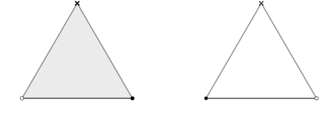
Figure 4. Oriented equilateral triangles as building blocks.

Remark 5.

(i) For each pair of adjacent triangles $T_{i}$ and $T_{j}$ with the common edge $a$ there exists a reflection $R_{a}\colon T_{i}\cup T_{j}\to T_{i}\cup T_{j}$, which interchanges $T_{i}$ with $T_{j}$, i.e, $R_{a}$ is an orientation-reversing isometry and fixes each point of the edge $a$.

(ii) Let $T_{i}$ be a black triangle and $\phi_{i}\colon T_{i}\to\overline{\mathbb{H}}^{+}$ a homeomorphism which preserves boundaries and is conformal in the interior and sends vertices $\circ,\bullet,\ast$ onto $0,1,\infty$, respectively.

If $T_{j}$ is a white triangle which is adjacent to $T_{i}$ with common edge $a$, we can extend continuously $\phi_{i}$ to a function $\Phi\colon T_{i}\cup T_{j}\to\hat{\mathbb{C}}$, which is defined in $T_{j}$ as $\Phi(x)=\overline{\phi_{i}\circ R_{a}(x)}$. By Schwarz reflection principle this function is holomorphic in the interior of $T_{i}\cup T_{j}$. We remark that it is a homeomorphism when restricted to $T_{j}$ and respects the decoration of its vertices ($\circ$ are zeros, $\bullet$ are in the pre-image of 1 and $\ast$ are poles). Analogously we can extend any homeomorphism $\phi_{j}\colon T_{j}\to\overline{\mathbb{H}}^{-}$, defined on a white triangle to a black triangle which is adjacent to it.

Construction of the Belyi function.

A surface with an equilateral decorated triangulation has associated a Belyi function constructed as follows: choose a black triangle $T_{i}$ and a homeomorphism $\phi_{i}\colon T_{i}\to\overline{\mathbb{H}}^{+}$ satisfying the hypothesis of Remark 5 (ii). Using the Schwarz reflection principle as in Remark 5 (i), we extend the function $\phi_{i}$ to the adjacent triangle to $T_{i}$ which shares a vertex decorated with the symbol $\circ$. We continue the process to another adjacent triangle until we use all the triangles which have the vertex $\circ$ in common (see Figure (5)). The function obtained by this process will be denoted as $\Phi$.

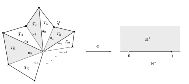
Figure 5. Extension $\Phi$ in a neighborhood of vertex $\circ$ of $T_{i}=T_{i1}$.

The function $\Phi$ is well-defined and holomorphic in the interior of $T_{i1}\cup\ldots\cup T_{in}$. It is also well-defined in the edge $a_{n}$ of the triangle $T_{i1}=T_{i}$ with vertices $\circ$ and $\bullet$. If $x\in a_{n}$, $\Phi(x)=\phi_{i}\circ R_{a_{1}}\circ\cdots\circ R_{a_{n-1}}(x)=\phi_{i}(x)$. The function $\phi_{i}$ extends continuously to a neighborhood of the white vertex $\circ=T_{i1}\cap\cdots\cap T_{in}$, and the extension is holomorphic in the interior. By construction $\Phi$ is conformal in the interior of each triangle.

Analogously, we make the extension around the black vertex $\bullet$ of $T_{i}$ and also the vertex $\ast$. We continue with this process to all triangles which are adjacent to those triangles where the function $\Phi$ has been defined until we do it for all the triangles of the euclidean decorated structure. This way we obtain a meromorphic function $\Phi\colon X\to\hat{\mathbb{C}}$ with critical values at the points $\{0,1,,\infty\}$. The construction of $\Phi$ implies that the pre-images of $0,1,\infty$ are decorated with the symbols $\circ,\bullet,\ast$, respectively. The black triangles correspond to the pre-images of the upper half-plane and the white triangles to the pre-images of the lower half-plane. The 1-skeleton of the triangulation corresponds to the pre-image of $\bar{\mathbb{R}}=\mathbb{R}\cup\{\infty\}$. We summarize all of the above by means of the following theorem (compare [Bost, ShVo90, VSh89]):

Theorem 3.

Let $X$ be a Riemann surface obtained by a decorated equilateral triangulation. Then there exists a Belyi function $f\colon X\to\hat{\mathbb{C}}$ such that the corresponding decorated triangulation coincides with the original.

This meromorphic function is equivalent to the continuous function $f\colon X\to 2\Delta$ which sends each triangle of $X$ to one of the two triangles of $2\Delta$, preserving the decoration.

2.5. Belyi function of a symmetric decorated triangulated structure

We observe that the proofs of the results of Section 2.4 remain valid if we weaken the condition that the triangles are equilateral to demanding only that condition (ii) in Remark 5 holds. Thus two triangles which share an edge are obtained from each other by a reflection along the edge. Such euclidean triangulations will be called symmetric. If the vertices of the triangulation are decorated by the symbols $\circ,\bullet,\ast$, then its triangles can be colored in a similar way to the previous case. The symmetric triangulations with such a decoration are called decorated symmetric triangulation (compare [CoItzWo94]).

Proposition 5.

(Compare [CoItzWo94] Theorem 2.) If $X$ is a compact Riemann surface given by a decorated symmetric triangulation, then there exists a Belyi function $f\colon X\to\hat{\mathbb{C}}$ which realizes the triangulation.

Corollary 1.

Let $X$ be a compact Riemann surface obtained from an equilateral triangulated structure. Then, given the barycentric subdivision there is a metric on $X$ in which all triangles in the subdivision are equilateral and the induced complex structure coincides with the original.

Proof.

By definition the complex structure given by the barycentric subdivision regarded as a euclidean triangulated structure coincides with the complex structure of $X$.

Let us decorate the vertices of the subdivision as follows: put the symbol $\bullet$ to all of the original vertices, assign the symbol $\circ$ to the midpoints of the edges and put the symbol $*$ to the barycenters. Then this triangulation is symmetric and therefore we have a decorated symmetric triangulation. By proposition 5 there exists a Belyi function $f:X\to\hat{\mathbb{C}}$ which realizes the triangulation.

If we consider the equilateral triangulated structure of the Riemann sphere by two triangles constructed at the beginning we can, using $f$, provide $X$ with a metric which renders all the triangles of the barycentric subdivision equilateral. This, in turn, induces a complex structure on $X$, since $f$ is conformal in the interior of each triangle. This complex structure coincides with the original. ∎

Example 1.

(The $j$-invariant) The following rational function of degree 6

(7) $$j(\lambda)=\frac{4}{27}\frac{(\lambda^{2}-\lambda+1)^{3}}{\lambda^{2}(\lambda-1)^{2}},$$

is called the $j$-invariant. The $j$-invariant has 8 critical points two zeros of order 3, 3 preimages of 1 with multiplicity 2 and three double poles. Its critical values are $\{0,1,\infty\}$, in other words it is a Belyi function. Its dessin d’enfant consists of two line segments which connect $\omega,1/2$ and $\omega^{-1},1/2$ and also by two circular arcs of radius 1 centered in 0 and 1 (see Figure (6)).

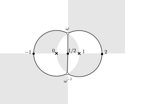
Figure 6. Dessin d’enfant of the $j$ invariant, where $\omega=\exp(2\pi i/6)$.

The function $j$ induces, via pull-back, a metric on the sphere in which all triangles are equilateral. This metric can be obtained by gluing euclidean equilateral triangles of the same size as shown in Figure (7).

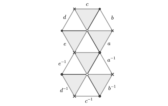
Figure 7. Equilateral triangulation of the Riemann sphere associated to the $j$-invariant.

In the previous paragraphs we constructed a Belyi function starting from an equilateral triangulation without assuming that the triangulation was decorated. If the triangulation is decorated we had a Belyi function $f$ that realizes the triangulation. Now we will show that the Belyi’s function associated to the barycentric subdivision is equivalent to the function $1-1/j(f)$. In other words it is obtained by post composing $j(f)$ with the Möbius function $z\mapsto 1-1/z$.

Let us start by describing the dessin d’enfant of $1-1/j(f)$. From the dessin of $j$ (see Figure (6)) we see that the decorated triangulation of $1-1/j$ is as in the dessin in Figure (8).

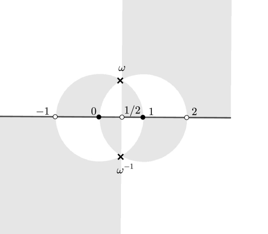
Figure 8. Dessin d’enfant of $1-1/j$.

Let $\mathcal{D}$ denote the dessin of $f$ and $\mathcal{T}$ the corresponding triangulation. The following simple observations about the dessin and triangulation of $1-1/j(f)$, are obtained by analyzing Figure (8):

• The vertices of the triangulation have the symbol $\bullet$ in the new dessin (including the poles)

• One adds a vertex with symbol $\circ$ in the interior of each edge of $\mathcal{D}$ (see Figure (9)).

• One adds a pole $\ast$ in each original triangle and the pole is connected with vertices in the boundary of the triangle with symbols $\bullet$ and $\circ$ described in (i) and (ii).

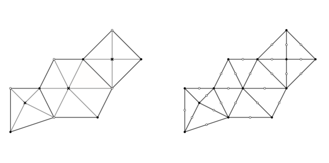
Figure 9. Dessin d’enfant of $1-1/j(f)$.

Therefore the dessin of $1-1/j(f)$ is precisely the dessin of the Belyi function corresponding to the barycentric subdivision. Hence such functions are equivalent. Summarizing we have the following proposition:

Proposition 6.

Let $X$ be a compact, connected Riemann surface obtained from a decorated equilateral triangulation and let $f\colon X\to\hat{\mathbb{C}}$ be the corresponding Belyi function. Then the Belyi function associated to the barycentric subdivision (decorated as in Corollary 1) is equivalent to $1-1/j(f)$.

3. Connected sum of two Belyi functions

3.1. Definition of the connected sum of two Bely functions

Let $f_{1}\colon X_{1}\to\hat{\mathbb{C}}$ and $f_{2}\colon X_{2}\to\hat{\mathbb{C}}$ be two Belyi functions and consider their corresponding equilateral decorated triangulations. Let $T_{1}^{+}$ be a black triangle of the triangulation of $f_{1}$ and $T_{2}^{-}$ a white triangle of the triangulation of $f_{2}$. We can construct the connected sum of $X_{1}$ with $X_{2}$ by removing the interior of $T_{1}^{+}$ and the interior of $T_{2}^{-}$ and glue the boundaries of $T_{1}^{+}$ and $T_{2}^{-}$ by the homeomorphism $f_{2}^{-1}\circ f_{1}\colon\partial T_{1}^{+}\to\partial T_{2}^{-}$. Denote such surface as $X_{1}\,{}_{{}_{T_{1}^{+}}}\#_{{}_{T_{2}^{-}}}\,X_{2}$.

The function $f_{1}\,{}_{{}_{T_{1}^{+}}}\#_{{}_{T_{2}^{-}}}\,f_{2}\colon X_{1}\,{}_{{}_{T_{1}^{+}}}\#_{{}_{T_{2}^{-}}}\,X_{2}\to\hat{\mathbb{C}}$ given by the formula

(8) $$f_{1}\,{}_{{}_{T_{1}^{+}}}\#_{{}_{T_{2}^{-}}}\,f_{2}(x)=\begin{cases}f_{1}(x),\ x\in X_{1}-\operatorname{int}T_{1}^{+}\\ f_{2}(x),\ x\in X_{2}-\operatorname{int}T_{2}^{-},\end{cases}$$

is well-defined and continuous.

By construction, the surface $X_{1}\,{}_{{}_{T_{1}^{+}}}\#_{{}_{T_{2}^{-}}}\,X_{2}$ has a decorated equilateral structure induced by the equilateral structures of $X_{1}$ and $X_{2}$ and with this structure it becomes a Riemann surface. The function (8) is holomorphic outside of $\partial T_{1}^{+}=\partial T_{2}^{-}$ in $X_{1}\,{}_{{}_{T_{1}^{+}}}\#_{{}_{T_{2}^{-}}}X_{2}$, and by continuity is holomorphic in the whole connected sum. Furthermore the function (8) is the function that realizes the triangulation in the connected sum.

Definition 3.

Consider the Belyi functions $f_{1}$ and $f_{2}$ and their associated triangulations. Given an edge $a_{1}$ of the dessin of $f_{1}$ and an edge $a_{2}$ of the dessin of $f_{2}$, there exists a unique black triangle $T_{1}$ which contains $a_{1}$ and a unique white triangle which contains $a_{2}$, therefore we can define $X_{1}\,{}_{{}_{a_{1}}}\#_{{}_{a_{2}}}\,X_{2}$ as $X_{1}\,{}_{{}_{T_{1}}}\#_{{}_{T_{2}}}\,X_{2}$.

Remark 6.

We will see in 3.2 that the connected sum of Belyi functions depends upon the chosen triangles used to perform the connected sum, in other words the ramified coverings corresponding to the connected sums could be non-isomorphic if we change the decorated triangles.

We don’t know if the conformal class of the Riemann surface $X_{1}\,{}_{{}_{T_{1}^{+}}}\#_{{}_{T_{2}^{-}}}\,X_{2}$ changes if we change the two decorated triangles along which the connected sum is performed.

3.2. Monodromy of the connected sum of two Belyi functions

Let $\sigma_{0}$, $\sigma_{1}$ be the cyclic permutations around the vertices of type $\circ$ and $\bullet$, respectively, for the function $f_{1}$, and let $\sigma_{0}^{\prime}$, $\sigma_{1}^{\prime}$ the corresponding permutations of $f_{2}$. Let us recall that such permutations determine the monodromy of the Belyi functions. Denote by $\sigma_{0}\,{}_{{}_{T_{1}^{+}}}\#_{{}_{T_{2}^{-}}}\,\sigma_{0}^{\prime}$ the permutation of the vertices $\circ$ of $f_{1}\,{}_{{}_{T_{1}^{+}}}\#_{{}_{T_{2}^{-}}}\,f_{2}$, and by $\sigma_{1}\,{}_{{}_{T_{1}^{+}}}\#_{{}_{T_{2}^{-}}}\,\sigma_{1}^{\prime}$ for the vertices $\bullet$.

Let us compute this permutations in order to determine the monodromy of $f_{1}\,{}_{{}_{T_{1}^{+}}}\#_{{}_{T_{2}^{-}}}\,f_{2}$.

Let $P_{0}$ and $Q_{0}$ the set of vertices with labels $\circ$ and $\bullet$, respectively, of the dessin determined by $f_{1}$ which are also vertices of $T_{1}^{+}$. Analogously let $P_{0}^{\prime}$ and $Q_{0}^{\prime}$ be the vertices with labels $\circ$ and $\bullet$, respectively, determined by the dessin of $f_{2}$ which are also vertices of triangle $T_{2}^{-}$ (see Figure (10)).

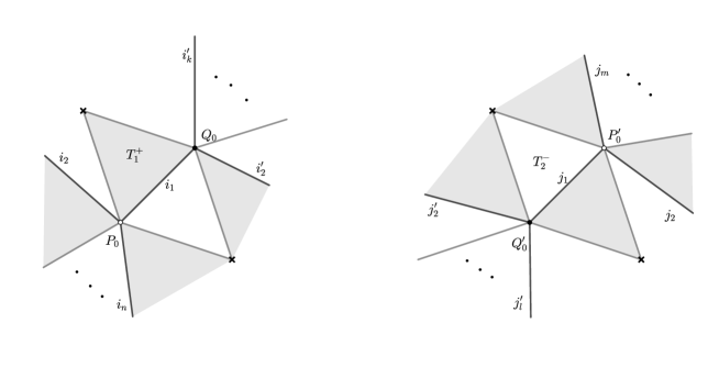
Figure 10. Permutation around the vertices.

In Figure (10) it is indicated the edges around the vertices (the positive orientation is counter-clockwise) and thus the figure also indicates the cyclic permutations around the vertices. Then we obtain:

• The cycle around $P_{0}=P_{0}^{\prime}$, in the connected sum, is given by the equation:

  $$(j_{1}\ j_{2}\ \ldots\ j_{m}\ i_{2}\ \ldots\ i_{n}).$$

  Since the other vertices with label $\circ$ remained unchanged when we make the connected sum the rest of the cycles of $\sigma_{0}\,{}_{{}_{T_{1}^{+}}}\#_{{}_{T_{2}^{-}}}\,\sigma_{0}^{\prime}$ remain the same.

• Analogously for $Q_{0}=Q_{0}^{\prime}$ in the connected sum, the cycle around it is

  $$(i_{1}\ i_{2}^{\prime}\ \ldots\ i_{k}^{\prime}\ j_{2}^{\prime}\ldots j_{l}^{\prime}),$$

  and the rest of the cycles of $\sigma_{1}\,{}_{{}_{T_{1}^{+}}}\#_{{}_{T_{2}^{-}}}\,\sigma_{1}^{\prime}$ remain the same.

Hence the permutations and monodromy of the Belyi function of the connected sum is completely described.

Remark 7.

(i) From the previous analysis we obtain the following formulas of the multiplicities and degree:

$$\operatorname{mult}_{P_{0}}(f_{1}\,{}_{{}_{T_{1}^{+}}}\#_{{}_{T_{2}^{-}}}\,f_{2}) = \operatorname{mult}_{P_{0}}f_{1}+\operatorname{mult}_{P_{0}^{\prime}}f_{2}-1$$

$$\operatorname{mult}_{Q_{0}}(f_{1}\,{}_{{}_{T_{1}^{+}}}\#_{{}_{T_{2}^{-}}}\,f_{2}) = \operatorname{mult}_{Q_{0}}f_{1}+\operatorname{mult}_{Q_{0}^{\prime}}f_{2}-1$$

$$\deg(f_{1}\,{}_{{}_{T_{1}^{+}}}\#_{{}_{T_{2}^{-}}}\,f_{2}) = \deg f_{1}+\deg f_{2}-1$$

The connected sum of two Belyi functions has as associated dessin d’enfant, it is obtained by the fusion of the corresponding edges of $T_{1}^{+}$ and $T_{2}^{-}$ which belong to the corresponding dessins.

Example 2.

Consider the polynomials

(9) $$f_{1}(z)=\frac{4^{4}}{3^{3}}z(1-z)^{3},\quad f_{2}(z)=4z(1-z)$$

whose dessin are in Figure (11). In Figure (12) we show the graphs corresponding to $f_{1}\,{}_{{}_{T_{1}^{+}}}\#_{{}_{T_{2}^{-}}}\,f_{2}$ and $f_{1}\,{}_{{}_{T_{2}^{+}}}\#_{{}_{T_{2}^{-}}}\,f_{2}$.

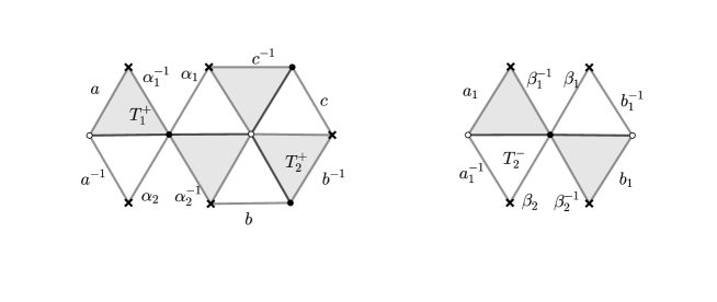
Figure 11. Dessins of $f_{1}(z)=\frac{4^{4}}{3^{3}}z(1-z)^{3},\quad f_{2}(z)=4z(1-z)$.

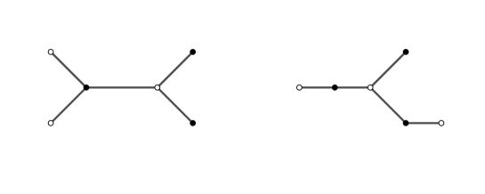
Figure 12. Graphs corresponding, respectively, to the dessins of $f_{1}\,{}_{{}_{T_{1}^{+}}}\#_{{}_{T_{2}^{-}}}f_{2}$ and $f_{1}\,{}_{{}_{T_{2}^{+}}}\#_{{}_{T_{2}^{-}}}\,f_{2}$.

From the previous formulas we see that, in general, the connected sum of Belyi functions depends upon the chosen triangles used in the connected sum (see Example 2). In 3.3 we give a condition in order to have the connected sum independent of the triangles.

In the following example we describe the connected sum of the $j$-invariant with itself.

Example 3 (Connected sum $j\#j$).

Consider the dessin of the $j$-invariant (see Figure (7)), and the connected sum $j\,{}_{{}_{T_{1}^{+}}}\#_{{}_{T_{2}^{-}}}\,j$, where $T_{1}^{+}$ and $T_{2}^{-}$ are indicated in Figure (13) with dotted lines.

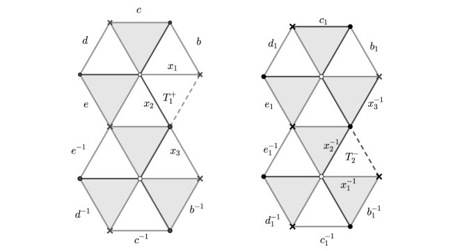
Figure 13. Dessin of $j\,{}_{{}_{T_{1}^{+}}}\#_{{}_{T_{2}^{-}}}\,j$.

When we glue to obtain the connected sum we obtain topologically the Riemann sphere with the decoration shown in Figure (14).

Figure 14. Visualization in the sphere of the connected sum $j\,{}_{{}_{T_{1}^{+}}}\#_{{}_{T_{2}^{-}}}\,j$.

3.3. Connected sum of Belyi functions which are Galois.

Let us recall that a meromorphic function $f\colon X\to\hat{\mathbb{C}}$ is of Galois type or regular if its group of deck transformations $\operatorname{Deck}(f)$ acts transitively on the fibers of the regular values of $f$ (see [For81]). Equivalently the unbranched covering, when we remove both the critical values and their pre-images, is a regular (or Galois) covering.

Remark 8.

If $f\colon X\to\hat{\mathbb{C}}$ is a Galois Belyi function, then the group of deck transformations $\operatorname{Deck}(f)$ acts transitively on the triangles of the same color and preserves the decoration of the vertices.

Proposition 7.

If $f_{1}\colon X_{1}\to\hat{\mathbb{C}}$ and $f_{2}\colon X_{2}\to\hat{\mathbb{C}}$ are two Belyi functions which are of Galois type Then, given $T_{1}^{+}$, $T_{1}^{\prime+}$ two black triangles of $X_{1}$ and $T_{2}^{-}$, $T_{2}^{\prime-}$ two white triangles of $X_{2}$, then there exists a biholomorphism

(10) $$\Phi\colon X_{1}\,{}_{{}_{T_{1}^{+}}}\#_{{}_{T_{2}^{-}}}\,X_{2}\to X_{1}\,{}_{{}_{T_{1}^{\prime+}}}\#_{{}_{T_{2}^{\prime-}}}\,X_{2}$$

for which the following diagram is commutative

(11)

Proof.

By Remark 8 there exists $\sigma_{1}\in\operatorname{Deck}(f_{1})$ and $\sigma_{2}\in\operatorname{Deck}(f_{2})$ such that $\sigma_{1}(T_{1}^{+})=T_{1}^{\prime+}$ and $\sigma_{2}(T_{2}^{-})=T_{2}^{\prime-}$ which preserve the decoration of the vertices (see Figure (15)).

Figure 15. Deck transformations preserve the decoration.

Let us define the map

(12) $$\sigma_{1}\,{}_{{}_{T_{1}^{+}}}\#_{{}_{T_{2}^{-}}}\,\sigma_{2}\colon X_{1}\,{}_{{}_{T_{1}^{+}}}\#_{{}_{T_{2}^{-}}}\,X_{2}\to X_{1}\,{}_{{}_{T_{1}^{\prime+}}}\#_{{}_{T_{2}^{\prime-}}}\,X_{2}$$

as follows:

(13) $$\sigma_{1}\,{}_{{}_{T_{1}^{+}}}\#_{{}_{T_{2}^{-}}}\,\sigma_{2}(x)=\begin{cases}\sigma_{1}(x),\ x\in X_{1}-\operatorname{int}T_{1}^{+}\\ \sigma_{2}(x),\ x\in X_{2}-\operatorname{int}T_{2}^{-}.\end{cases}$$

This function is well-defined because if $x\in\partial T_{1}^{+}$, $y\in\partial T_{2}^{-}$ are such that tal que $x\sim y$, then $f_{1}(x)=f_{2}(y)$. Hence $f_{1}(\sigma(x))=f_{2}(\sigma(y))$, therefore $\sigma(x)\sim\sigma(y)$. In addition, $\sigma_{1}\,{}_{{}_{T_{1}^{+}}}\#_{{}_{T_{2}^{-}}}\,\sigma_{2}$ is a homeomorphism.

Clearly $\sigma_{1}\,{}_{{}_{T_{1}^{+}}}\#_{{}_{T_{2}^{-}}}\,\sigma_{2}$ is conformal in the complement of $\partial T_{1}^{+}=\partial T_{2}^{-}$ and, by continuity, such function can be extended conformally to all of the connected sum.

The diagram (11) commutes because

$$(f_{1}\,{}_{{}_{T_{1}^{\prime+}}}\#_{{}_{T_{2}^{\prime-}}}\,f_{2})\circ(\sigma_{1}\,{}_{{}_{T_{1}^{+}}}\#_{{}_{T_{2}^{-}}}\,\sigma_{2})(x) = (f_{1}\circ\sigma_{1})\,{}_{{}_{T_{1}^{+}}}\#_{{}_{T_{2}^{-}}}\,(f_{2}\circ\sigma_{2})(x)$$

$$= f_{1}\,{}_{{}_{T_{1}^{+}}}\#_{{}_{T_{2}^{-}}}\,f_{2}(x).$$

∎

3.4. Connected sum of the polynomials $z^{m}$.

Since the monomial functions of the form $z^{m}$, with $m\geq 1$, are of Galois type their connected sum does not depend on the triangles chosen to do the connected sum. Thus in this case we denote the connected sum simply as $z^{m}\#z^{n}$.

From what was discussed before one has that the connected sum $z^{m}\#z^{n}$ has the same monodromy as that of the function $z\mapsto{z^{m+n-1}}$. Hence, up to isomorphism of ramified coverings one has:

(14) $$z^{m}\#z^{n}=z^{m+n-1}.$$

Therefore we have the following properties:

• Associativity: $(z^{m}\#z^{n})\#z^{k}=z^{m+n+k-2}=z^{m}\#(z^{n}\#z^{k})$.

• There exists a neutral element: the polynomial $z$.

• Commutativity.

Then the Belyi functions of the form $z^{m}$ is, under connected sum, a commutative monoid (under equivalence relations of ramified coverings). Figure (16) illustrates the connected sum of $z^{3}$ with $z^{2}$.

Remark 9.

The connected sum of two polynomials of the form $z^{m}$, with $m$ odd is a closed operation.

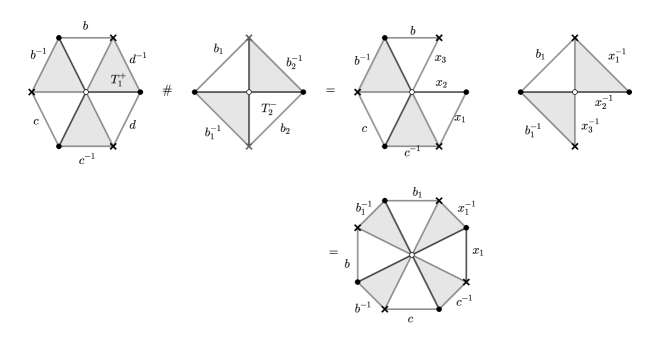
Figure 16. Connected sum of $z^{3}$ with $z^{2}$, represented topologically by identifying polygons.

Remark 10 (Shabat polynomials).

A polynomial which is a Belyi function has as dessin d’enfant associated a bicolored tree and reciprocally, given a bicolored tree there exists a Belyi function that realizes it. Such polynomials are called Shabat polynomials (see [ShZv94]).

The dessin of a connected sum of two Shabat polynomials is again a bicolored tree since the connected sum does not create cycles in the dessin of the connected sum. Hence the connected sum of two Shabat polynomials is again a Shabat polynomial (under the isomorphism class of branched coverings)

3.5. Connected sum of double-star polynomials.

Double-star polynomials are graphs like the one in self-explicatory Figure (17). These dessins can be realized by polynomials of the form:

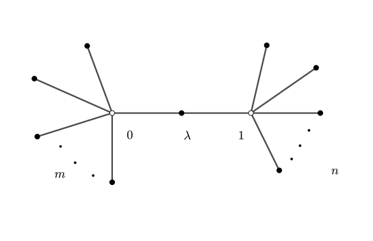
Figure 17. Double-star tree corresponding to $P_{m,n}$.

(15) $$P_{m,n}(z)=\mu z^{m}(1-z)^{n},\quad\mu=\frac{(m+n)^{m+n}}{m^{m}n^{n}},\quad\lambda=\frac{m}{m+n},\quad m,n\geq 1.$$

Let $a$ and $b$ denote the intervals $[0,\lambda]$ and $[\lambda,1]$, respectively, and $a_{1}$, $b_{1}$ the intervals $[-1,0]$ and $[0,1]$ respectively. Then:

(16) $$z^{m}\,{}_{a}\#_{a_{1}}\,(1-z^{2})\,{}_{b_{1}}\#_{b}\,z^{n}=P_{m,n}(z)\quad\text{(because they have the same dessin.)}$$

3.6. Connected sum of Tchebychev polynomials

Recall that Tchebychev polynomials are those polynomials $\bar{T}_{n}\,\,(n\in\mathbb{Z},n\geq 0)$ that satisfy the functional identity:

(17) $$\bar{T}_{n}(\cos\ z)=\cos\ nz.$$

Using De Moivre’s formula it is possible to calculate them explicitly. In fact they have the satisfy the recursive formula for $n=0$, $\bar{T}_{0}(x)=1$. For $n\geq 1$

(18) $$\bar{T}_{n}(x)=2x\bar{T}_{n-1}(x)-\bar{T}_{n-2}(x).$$

This implies that $\bar{T}_{n}$ has degree $n$.

The critical points of the polynomial $\bar{T}_{n}(x)$ are $\cos k\pi/n$, with $k=1,\ldots,n-1$, therefore the critical values are

(19) $$\bar{T}_{n}\left(\cos\ \frac{k\pi}{n}\right)=\cos\ k\pi=\begin{cases}-1,\ k\ \text{odd}\\ 1,\ k\ \text{even},\quad k=1,\ldots,n-1.\end{cases}$$

Hence $\bar{T}$ has only three critical values. The function

(20) $$T_{n}(z)=\frac{1}{2}(\bar{T}_{n}(z)+1)$$

is a Belyi function for each $n\geq 1$ with critical values 0, 1 and $\infty$.

The dessins of these functions are depicted in Figure (18).

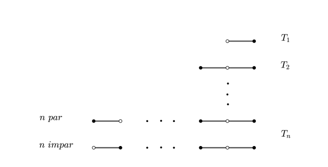
Figure 18. Dessins of Tchebychev polynomials ${T}_{n}$. All these dessins have as extreme points $-1$ and $1$, and vertices in $cos\ k\pi/n$.

The dessins of the Belyi Tchebychev polynomials $T_{k}$, with $n\geq 2$, have two distinguished edges, namely those at the extremes. From these dessins of each connected sum we obtain the following identities:

(21) $$\begin{cases}T_{l}\#T_{m}=T_{l+m-1},\quad m\ \text{odd},\\ (1-T_{l})\#T_{m}=T_{l+m-1},\quad m\ \text{even},\\ T_{l}\#(1-T_{m})=1-T_{l+m-1},\quad m\ \text{even},\end{cases}$$

where the connected sum is taken with respect to the extremal edges; the one on the right for the first function and the one on the left for the second function. From (21) one obtains:

Proposition 8.

If $n$ is odd $T_{2}\#T_{n}=T_{n+1}$, if $n$ even $(1-T_{2})\#T_{n}=T_{n+1}$. Hence,

(22) $$\begin{cases}T_{n}=(1-T_{2})\#\cdots\#T_{2}\#(1-T_{2})\#T_{2},\ n\ \text{impar},\\ T_{n}=T_{2}\#\cdots\#T_{2}\#(1-T_{2})\#T_{2},\ n\ \text{par},\end{cases}$$

where both sums consist of $n-1$ summands. Equivalently,

(23) $$\begin{cases}T_{n}=((1-T_{2})\#T_{2})^{\#\frac{n-1}{2}}=T_{3}^{\#\frac{n-1}{2}},\ n\ \text{impar},\\ T_{n}=T_{2}\#T_{n-1}=T_{2}\#(T_{3}^{\#\frac{n-2}{2}}),\ n\ \text{par}.\end{cases}$$

Remark 11.

From (21) it follows that the connected sum is a closed operation for the Tchebychev polynomials of odd degree. In addition they form a commutative monoid. From (23) it follows that this monoid is generated by $T_{3}$.

3.7. Connected sum of surfaces with an equilateral triangulation

Let $X_{1}$ and $X_{2}$ be Riemann surfaces obtained by equilateral triangulations. Let $T_{1}$ and $T_{2}$ be two triangles in $X_{1}$ and $X_{2}$, respectively. Suppose the triangles are decorated with the symbols $(\circ,\bullet,\ast)$ in such a way that such a decoration induces a positive orientation in $T_{1}$ and a negative orientation in $T_{2}$. Consider the connected sum $X_{1}\,{}_{{}_{T_{1}}}\#_{{}_{T_{2}}}\,X_{2}$, where the gluing homeomorphism is the isometry from the boundary of $T_{1}$ to the boundary of $T_{2}$ which preserves the decoration. As explained before, $X_{1}\,{}_{{}_{T_{1}}}\#_{{}_{T_{2}}}\,X_{2}$ has also a decorated equilateral structure, which gives the connected sum the structure of an arithmetic Riemann surface.

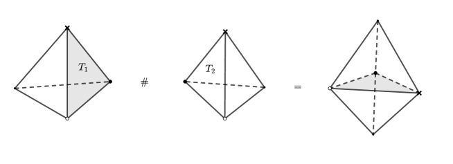
Figure 19. Connected sum of two tetrahedra.

The connected sum defined in the previous paragraph is compatible with the definition of connected sum of Belyi functions since the gluing map of $f_{2}^{-1}\circ f_{1}$ in the connected sum preserves the decoration and it is an isometry which reverses the orientation of the boundaries since $f_{2}^{-1}\circ f_{1}(x)=f_{2}^{-1}\circ\bar{f_{1}}(x)$, for all $x\in\partial T_{1}$.

Figure (19) shows an example of the connected sum of two surfaces with equilateral triangulations.

3.8. Flips

Another way to define the connected sum of two triangulated surfaces can be done if instead of removing the interior of a triangle in each surface we remove rhombi i.e, removing pairs of adjacent triangles. Let $R_{1}$ and $R_{2}$ be two rhombi in $X_{1}$ and $X_{2}$, respectively, and suppose that a triangle in each of the rhombi is decorated with the symbols $(\circ,\bullet,\ast)$ in such a way that the decoration induces a positive orientation in $R_{1}$ and a negative orientation in $R_{2}$, then we can construct the connected sum $X_{1}\,{}_{{}_{R_{1}}}\#_{{}_{R_{2}}}\,X_{2}$, where the gluing map is an isometry from $\partial{R_{1}}$ to $\partial{R_{2}}$ which respects the decoration of the triangles.

Given a decorated equilateral triangulated structure on a surface $X$ if we perform the connected sum with a tetrahedron along a rhombus the triangulation of the connected sum is obtained from the triangulation of $X$ by flipping the diagonals of the rhombus (figure 20 shows an example). Any two simplicial triangulations of $X$ with the same, and sufficiently large, number of vertices can be transformed into each other, up to homeomorphism, by a finite sequence of diagonal flips [BNN95]. If $P(X,n)$ denotes the set of simplicial triangulations of $X$ with $n$ vertices these triangulations are permuted by flippings.

Question.

What are the fields of definition of the algebraic curves corresponding to the triangulated surfaces of the different permutations under fliping?

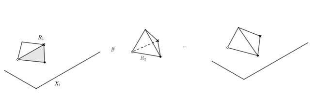
Figure 20. Connected sum of a surface and a regular tetrahedron using rhombi.

3.9. Connected sum with tetrahedra and elementary sub-divisions (starrings)

In this subsection we will make some elementary observations on the relations between starrings and connected sums of tetrahedra. A triangulation on a surface can be subdivided (or refined) by means of some elementary operations called starrings. Starting from an equilateral triangulation we can apply this refinement and obtain a new equilateral triangulation (by declaring all triangles equilateral of the same size) which induces a new flat metric with conic singularities.

Remark 12.

In general we don’t know how the complex structure changes nor the algebraic subfield of definition, as a subfield of $\bar{\mathbb{Q}}$.

Let $X$ be a regular tetrahedron with its complex structure induced by the triangulation. Suppose that one of its triangles $T_{2}$ is negatively oriented with respect to the decoration $(\circ,\bullet,\ast)$. Let $X_{1}$ be a Riemann surface obtained from an equilateral structure and let $T_{1}$ be a triangle which positively oriented with the decoration $(\circ,\bullet,\ast)$. Then, combinatorially, the Riemann surface $X_{1}\,{}_{{}_{T_{1}}}\#_{{}_{T_{2}}}\,X_{2}$, is obtained from $X_{1}$ by starring $T_{2}$ by an interior point (see Figure (21)).

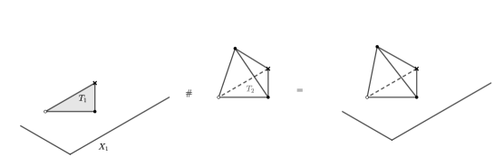
Figure 21. Connected sum of a triangulated surface with a tetrahedron. Combinatorially this corresponds to starring with respect to a point in the interior of a triangle.

Analogously, if we make the connected sum of two tetrahedra we obtain a doble pyramid with six triangles $2P$ (see Figure (19)) and consider a rhombus $R_{2}$ obtained from two triangles with a triangle in each tetrahedron in this connected sum. If $R_{1}$ is a rhombus in $X_{1}$ obtained from two adjacent triangles we can do the connected sum $X_{1}\,{}_{{}_{R_{1}}}\#_{{}_{R_{2}}}\,2P$ to obtain a triangulated Riemann surface which is combinatorially the starring of the triangulation of $X_{1}$ with respect to the midpoint of an edge of $T_{1}$ (see Figure (22)).

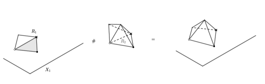
Figure 22. Connected sum of a triangulated surface with a tetrahedron using rhombi. Combinatorially, this corresponds to starring with respect to a point in the interior of an edge.

4. Elliptic curves with a hexagonal decomposition

4.1. Coverings of elliptic curves and orbits of $\operatorname{PSL}(2,\mathbb{Q})$ in the upper half-plane.

Proposition 9.

Let $\Lambda$ be a lattice in $\mathbb{C}$. Then a Riemann surface $X$, is a non-ramified holomorphic covering of $\mathbb{C}/\Lambda$ if and only if $X$ is conformally equivalent to $\mathbb{C}/\Gamma$ for some sub-lattice $\Gamma\leq\Lambda$.

Proof.

If $\Gamma\leq\Lambda$ is a sub-lattice one has the following commutative diagram

(24)

where $\pi_{\Gamma}$ and $\pi_{\Lambda}$ are the natural projection to the quotients and $\Phi$ is the function that changes the equivalence relation. It follows from (24) that $\Phi$ is a holomorphic map and, by Riemann-Hurwitz formula is not ramified.

Reciprocally, if there exists $f\colon X\to\mathbb{C}/\Lambda$ a non-ramified holomorphic covering the group of deck transformations of the covering $\operatorname{Deck}(f)$ is a sub-lattice of $\Lambda$ and $X$ is conformally equivalent to $X/\operatorname{Deck}(f)$. Then we can take $\Gamma=\operatorname{Deck}(f)$.

∎

Proposition 10.

If $\tau$ and $\tau^{\prime}\in\mathbb{H}$, then $X_{\tau^{\prime}}$ is a holomorphic covering of $X_{\tau}$ if and only if there exists $\gamma\in\operatorname{PSL}(2,\mathbb{Q})$such that $\tau^{\prime}=\gamma(\tau)$.

Proof.

If $X_{\tau^{\prime}}$ is a holomorphic covering of $X_{\tau}$, there exists a sub-lattice $\Gamma=\langle\omega_{1},\omega_{2}\rangle$ of $\langle 1,\tau\rangle$, such that $X_{\tau^{\prime}}$ is conformally equivalent to $\mathbb{C}/\Gamma$. We can assume that $\omega_{1}/\omega_{2}\in\mathbb{H}$. Then there exist $a,b,c,d\in\mathbb{Z}$ such that

(25) $$\left(\begin{matrix}\omega_{1}\\ \omega_{2}\end{matrix}\right)=\left(\begin{matrix}a&b\\ c&d\end{matrix}\right)\left(\begin{matrix}1\\ \tau\end{matrix}\right),\quad ad-bc\neq 0,$$

therefore $\gamma(z)=(az+b)/(cz+d)$ is in $\operatorname{PSL}(2,\mathbb{Q})$ and $\gamma(\tau)=\omega_{1}/\omega_{2}$. On the other hand, $\omega_{1}/\omega_{2}$ is in the orbit of $\tau^{\prime}$ under $\operatorname{PSL}(2,\mathbb{Z})$, because the associated elliptic curves are conformally equivalent. Hence $\tau^{\prime}$ is in the orbit of $\tau$ under $\operatorname{PSL}(2,\mathbb{Q})$.

Reciprocally, suppose there exists $\gamma\in\operatorname{PSL(2,\mathbb{Q})}$ such that $\gamma(\tau)=\tau^{\prime}$. Clearing denominators we can assume that

(26) $$\gamma(z)=\frac{az+b}{cz+d},\quad\text{con}\ a,b,c,d\in\mathbb{Z}\ \text{y}\ ad-bc\neq 0.$$

Therefore if we define $\omega_{1}=a\tau+b$ and $\omega_{2}=c\tau+d$ we have $\Gamma=\langle\omega_{1},\omega_{2}\rangle\leq\langle 1,\tau\rangle$. Hence $\mathbb{C}/\Gamma$ is a holomorphic covering of $X_{\tau}$. Since $\tau^{\prime}=\omega_{1}/\omega_{2}$, $\mathbb{C}/\Gamma$ is isomorphic to $X_{\tau^{\prime}}$ and the result follows. ∎

By the previous results and Belyi’s Theorem we obtain:

Corollary 2.

If $\tau\in\mathbb{H}$ is such that $X_{\tau}$ is an arithmetic elliptic curve (i.e, defined over $\bar{\mathbb{Q}})$ then for any $\gamma\in\operatorname{PSL}(2,\mathbb{Q})$, $X_{\gamma(\tau)}$ is also arithmetic.

Corollary 3.

If $\tau$ and $\tau^{\prime}\in\mathbb{H}$, then $X_{\tau^{\prime}}$ is a holomorphic covering of $X_{\tau}$ if and only if $X_{\tau}$ is a holomorphic covering of $X_{\tau^{\prime}}$.

Corollary 3 can also be deduced as follows: suppose that $X_{\tau^{\prime}}$ is a holomorphic covering of $X_{\tau}$, then $X_{\tau^{\prime}}\cong\mathbb{C}/\Gamma$ for some sub-lattice $\Gamma=\langle\omega_{1},\omega_{2}\rangle\leq\langle 1,\tau\rangle$. By Remark 13 there exists $k\in\mathbb{Z}$ such that $k\langle 1,\tau\rangle\leq\langle\omega_{1},\omega_{2}\rangle$. Since the elliptic curve $X_{\tau}$ is isomorphic to $\mathbb{C}/\langle k,k\tau\rangle$, it follows that $X_{\tau}$ is a holomorphic covering of $X_{\tau^{\prime}}$.

Remark 13.

If $\langle\omega_{1},\omega_{2}\rangle\leq\langle 1,\tau\rangle$ is una sub-lattice, then there exists $k\in\mathbb{Z}$ such that $k\langle 1,\tau\rangle\leq\langle\omega_{1},\omega_{2}\rangle$. This is because there is a matrix which satisfies (25), then if we take $k=ad-bc$ we obtain:

(27) $$k\left(\begin{matrix}1\\ \tau\end{matrix}\right)=\left(\begin{matrix}d&-b\\ -c&a\end{matrix}\right)\left(\begin{matrix}\omega_{1}\\ \omega_{2}\end{matrix}\right).$$

4.2. Surfaces which admit a regular hexagonal decomposition

Proposition 11.

If $\Gamma$ is a torsion-free subgroup of the triangular group $\Gamma_{2,3,6}$, then $\Gamma$ is a sub-lattice of $\Lambda_{1,\omega}$, where $\omega$ is equal to $\exp(2\pi i/6)$.

Proof.

Consider the action of $\Gamma_{2,3,6}$ on the complex plane $\mathbb{C}$ and its associated tessellation (see Figure (23)). We note that the only points in $\mathbb{C}$ with nontrivial stabilizer are the vertices of the tessellation. Therefore, if $T\in\Gamma_{2,3,6}$ has a fixed point, $T$ must belong to the stabilizer of some vertex, however these stabilizer are cyclic hence $T$ is a torsion element.

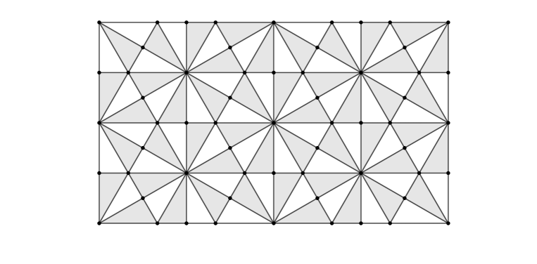
Figure 23. Tessellation of $\mathbb{C}$ by the triangular group $\Gamma_{2,3,6}$.

On the other hand, if $T\in\Gamma_{2,3,6}$ is a translation $T$ then it sends vertices of the tessellation into vertices of the tessellation and it preserves its valencies, hence it preserves the triangular lattice $\Lambda_{1,\omega}$ (the points of these triangular lattice are the vertices with valence 12).

It follows that if $\gamma$ is in the torsion-free subgroup $\Gamma$, then $\gamma$ must be a translation that preserves the triangular lattice. Hence $\gamma\in\Lambda_{1,\omega}$. ∎

Proposition 12.

Suppose that $X$ is a compact, connected Riemann surface. Then $X$ admits a flat structure given by a finite union of regular hexagons (i.e, the valence of each vertex is 3) if and only if $X$ is conformally equivalent to $\mathbb{C}/\Gamma$, where $\Gamma$ is a sub-lattice of $\Lambda_{1,\omega}$.

Proof.

Let us suppose that $X$ is given by a cellular decomposition by regular hexagons, with vertices of valence 3 so that the surface doesn’t have singularities. Let us decorate with the symbol $\bullet$ the vertices (the 0-cells), with the symbol $\circ$ the midpoints of the edges. Let us define new edges dividing in half each edge of the hexagons. This cartographic map is a uniform dessin d’enfant with valence $(2,3,6)$. Hence $X$ is conformally equivalent to $\mathbb{C}/\Gamma$ for some torsion-free subgroup (see [GG12] section 4.4.3) $\Gamma\leq\Gamma_{2,3,6}$. By Proposition 11 this subgroup must be a sub-lattice of $\Lambda_{1,\omega}$.

Reciprocally, let us suppose that $\Gamma$ is a sub-lattice of $\Lambda_{1,\omega}$ with $\omega=\exp(2\pi{i}/6)$. By Proposition 9 the map $\Phi\colon\mathbb{C}/\Gamma\to\mathbb{C}/\Lambda$ is a holomorphic covering map. Therefore any regular hexagonal decomposition of $\mathbb{C}/\Lambda$ lifts, by means of $\Phi$, to endow $\mathbb{C}/\Gamma$ with a regular hexagonal decomposition.The complex structure induced by the hexagonal structure coincides with original complex structure since $\Phi$ is holomorphic. ∎

Remark 14.

(i) The elliptic curve $\mathbb{C}/\Lambda_{1,\omega}$, with $\omega=\exp(2\pi i/6)$, admits hexagonal decompositions, it even admits decompositions such that two hexagons intersect in at most one edge, see Figure (24).

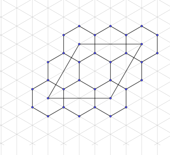
Figure 24. Hexagonal decomposition of $\mathbb{C}/\Lambda_{1,\omega}$.

(ii) In the proof of proposition 12 we didn’t need to suppose that the hexagons meet at most at one edge. For instance the decomposition could consist of only one hexagon.

Propositions 9 10, 12 imply the following corollary.

Corollary 4.

Let $\tau\in\mathbb{H}$, then $X_{1,\tau}$ admits a flat structure without conical points given by a finite union of regular hexagons with each vertex of valence 3 if and only if there exists $\gamma\in\operatorname{PSL}(2,\mathbb{Q})$ such that $\tau=\gamma(\omega)$.

5. Geodesics in surfaces with a decorated equilateral triangulation

As mentioned before we will denote by $\Delta$ the euclidean equilateral triangle with vertices at $0,1,\omega$, with $\omega=\exp(2\pi i/6)$. We decorate these vertices with the symbols $\circ,\bullet$ and $\ast$, respectively. All through this paper we will assume that the vertices of the tessellation of the triangular group $\Gamma_{3,3,3}$, generated by $\Delta$ are decorated in a compatible way with respect to $\Delta$ (see Figure (25)).

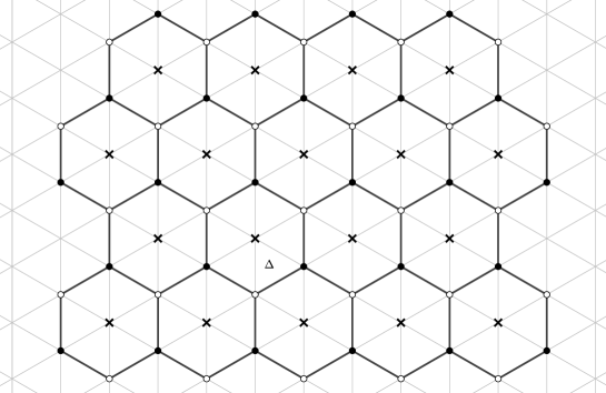
Figure 25. Decorated tessellation of $\Gamma_{3,3,3}$, generated by $\Delta$.

All through this section we will suppose that $X$ is a Riemann surface obtained from a decorated euclidean equilateral triangulation, (in other words $X$ is determined from a dessin d’enfant). Let $f\colon X\to 2\Delta$ be its associated Belyi function. Let us recall that, by definition, this function is the one that sends each triangle of $X$ to one of the two triangles of $2\Delta$, preserving the decoration.

This section is devoted to the study of geodesics with the respect to the conic flat metric of the triangulated surface $X$ and which do not pass through the of the vertices of the triangulation.

5.1. Geodesics defined by straight lines

Let $\ell$ be a straight line in $\mathbb{C}$ which passes through $1/2$ and does not contain any point of the lattice $\Lambda_{1,\omega}$. Let $P$ be the union of all the triangles which intersect $\ell$. Then since $\ell$ does not contain any point of the lattice $\ell$ is contained in the interior of $P$. In all that follows we will assume that $P$ has its vertices decorated according to the decoration given to the tessellation associated to $\Gamma_{3,3,3}$ (see Figure (26)).

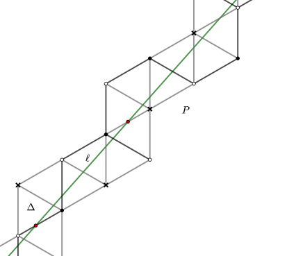
Figure 26. Decorated triangle and straight line $\gamma$ passing through $1/2$.

Let $p\in{X}$ be the midpoint of an edge of the dessin of $X$ determined by $f$, i.e, $p\in f^{-1}(1/2)$. Then there exist a unique continuous map $\Psi\colon P\to X$ satisfying the following conditions:

• $\Psi(1/2)=p$.

• $\Psi$ sends isometrically triangles onto triangles through an isometry that preserves the decoration.

Then the images under $\Psi$ of two adjacent triangles of $P$, are two adjacent triangles in $X$. Therefore $\Psi$ is a local isometry from the interior of $P$ to $X$. We will call the map $\Psi$ the development of $\ell$ in $X$ with respect to $p$.

By the previous observations $\Psi(\ell)$ is a geometric geodesic in $X$ (i.e, a non parametrized geodesic). We we call such a curve $\Psi(\ell)$ the geometric geodesic induced by $\ell$ in $X$ .

Remark 15.

We observe that $2\Delta$ is the quotient $\mathbb{C}/\Gamma_{3,3,3}$. So that the complex plane $\mathbb{C}$ is a branched covering of $2\Delta$ with branching points the vertices of the triangles determined by $\Gamma_{3,3,3}$. The natural projection $\pi\colon\mathbb{C}\to\mathbb{C}/\Gamma_{3,3,3}$ is an isometry when restricted to each triangle and it preserves the decorations. This implies that $\pi(\ell)$ is a geometric geodesic in $2\Delta$. In fact if $X=2\Delta$ and $p=1/2\in 2\Delta$ then $\pi_{|_{P}}=\Psi$.

Remark 16.

Let us denote $\Psi(\ell)$ by $\tilde{\gamma}$ and $\pi(\ell)$ by $\gamma$. By Remark 15 it follows that locally $f\colon X\to 2\Delta$ can be written as $f=\pi\circ\Psi^{-1}$. Hence, $\tilde{\gamma}$ is the lifting, based in $p$, of $\gamma$, with respect to $f$.

5.2. Closed and primitive geodesics in $2\Delta$

Let us consider the parametrized straight line $\ell(t)=1/2+t\omega_{0}$, with $\omega_{0}\in\Lambda_{1,\omega}$ (the parametrization is by a multiple of arc-length). We study in this subsection the condition we must impose to $\omega_{0}$, which guarantee that $\ell(t)$ induces a smooth closed geodesic in $2\Delta$ which does not contain any vertex of $2\Delta$.

The following simple proposition, whose proof we leave to the reader, determines the condition that garantes that $\ell$ does not contain any point of the lattice $\Lambda_{1,\omega}$.

Proposition 13.

If $\omega_{0}\in\Lambda_{1,\omega}$ is expressed as $\omega_{0}=m_{0}+n_{0}\omega$, with $n_{0}\neq 0$, then the parametrized line $\ell(t)=1/2+t\omega_{0}$ does not contain any point of the lattice $\Lambda_{1,\omega}$ if and only if the diophantine equation $n_{0}=(2n_{0})x+(-2m_{0})y$ has a solution with $x,y\in{\mathbb{Z}}$.

Corollary 5.

If $\omega_{0}=m+n\omega\in\Lambda_{1,\omega}$ with $\text{gcd}(m,n)=1$, then $\ell(t)=1/2+t\omega_{0}$ does not contain a point in the lattice $\Lambda_{1,\omega}$ if and only if $n$ is odd.

Remark 17.

Let $Hex=\Gamma_{3,3,3}\cap\Lambda_{1,\omega}$. We observe that $Hex$ is the sub-lattice of $\Lambda_{1,\omega}$ consisting of the vertices with symbol $\circ$ of the tessellation obtained by $\Gamma_{3,3,3}$. We see that $\omega_{1}=2-\omega$ and $\omega_{2}=1+\omega$ are $\mathbb{R}$-linearly independent vectors wich belong to $Hex$ (see Figure (27). Then

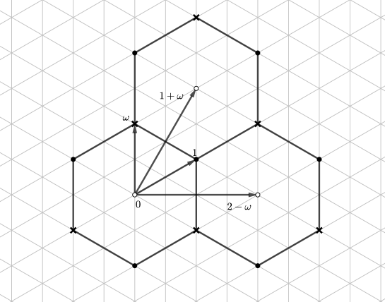
Figure 27. Generators of the sub-lattice formed by the vertices with symbol $\circ$.

(28) $$Hex=\langle 2-\omega,\ 1+\omega\rangle,$$

Therefore any element $\alpha$ of $Hex$ can be written in terms of the base $1,\ \omega$ as follows

(29) $$\alpha=m\omega_{1}+n\omega_{2}=2m+n+(n-m)\omega.$$

Remark 18.

If $\omega_{0}=m+n\omega\in\Lambda_{1,\omega}$, then $3\omega_{0}\in Hex$, because

(30) $$3(m+n\omega)=(m-n)(2-\omega)+(m+n)(1+\omega).$$

In addition, if $2\omega_{0}=2(m+n\omega)\in Hex$, then $\omega_{0}\in Hex$.

As a consequence of what has been proved in this subsection we have the following theorem that gives conditions in order that the parametrized (by a multiple constant of arc-length) $\ell(t)=1/2+t\omega_{0}$ parametrizes a primitive closed geodesic in $2\Delta$.

Theorem 4.

Let $\omega_{0}=m+n\omega$, with $m$ and $n$ relatively prime and $n$ odd. Let $\ell(t)=1/2+t\omega_{0}$. If $\omega_{0}\in Hex$, then the curve $\gamma(t)=\pi(\ell(t))$ with $t\in[0,1]$ is a primitive closed geodesic in $2\Delta$. If $\omega_{0}\notin Hex$, $\gamma(t)=\pi(\ell(t))$ with $t\in[0,3]$, is a primitive closed geodesic in $2\Delta$.

Corollary 6.

The length of the geodesic $\gamma$ parametrized by $\pi(\ell(t))=\pi(1/2+t\omega_{0})$, $\omega_{0}=m+n\omega$ with $\text{gcd}(m,n)=1$ and $n$ odd, is equal to

(31) $$\operatorname{length}\gamma=\begin{cases}|\omega_{0}|,\ \text{if}\ \omega_{0}\in Hex,\\ 3|\omega_{0}|,\ \text{if}\ \omega_{0}\notin Hex.\end{cases}$$

The following is the reciprocal of Theorem 4: Let $\gamma$ be a closed smooth geodesic in $2\Delta$ based on $1/2$ and not passing through any vertex); let $\ell$ be its lifting with respect to the canonical projection $\pi\colon\mathbb{C}\to\mathbb{C}/\Gamma_{3,3,3}$, with base point $1/2$ (the lifting exists because $\pi$ is a covering map outside of the vertices of the tessellation). Since $\pi$ is a local isometry outside of the vertices $\ell$ is also a geodesic (with the euclidean metric of $\mathbb{C}$) which passes through $1/2$ and it does not contain any vertex of the tessellation given by $\Gamma_{3,3,3}$. Hence $\ell$ is a straight line which does not contain points in $\Lambda_{1,\omega}$. Since the image of $\ell$ under $\pi$ is closed curve it must connect $1/2$ with $1/2+\omega_{0}^{\prime}$, for some $\omega_{0}^{\prime}\in\Gamma_{3,3,3}$. Since $\pi$ is a local Riemannian isometry outside of the vertices the angles between the straight line and the edges which contain $1/2$ and $1/2+\omega_{0}^{\prime}$ are the same and, therefore the edges are parallel and $\omega_{0}^{\prime}\in\Lambda_{1,\omega}$. Hence $\omega_{0}^{\prime}$ is a vertex with symbol $\circ$ of the decorated tessellation determined by $\Gamma_{3,3,3}$.

Proposition 14 implies that we can choose $\omega_{0}=m_{0}+n_{0}\omega$ with minimal modulus which generates the same straight line as $\omega_{0}^{\prime}$. Then $\text{gcd}(m_{0},n_{0})=1$ and since $\ell$ does not contain points in the lattice it follows that $n_{0}$ is odd. We summarize all of the above paragraph with the following:

Theorem 5.

A smooth closed curve $\gamma(t)$ en $2\Delta$, which passes through $1/2$, is a parametrized (by a constant multiple of arc-length) primitive closed geodesic in $2\Delta$ if and only if $\gamma(t)$ is given by $\pi(\ell(t))=\pi(1/2+t\omega_{0})$ as in Theorem 4.

Proposition 14.

Let $\omega_{0}=m_{0}+n_{0}\omega$ with $\text{gcd}(m_{0},n_{0})=1$. Then the intersection of the line $\ell(t)=t\omega_{0}$ with the lattice $\Lambda_{1,\omega}$ is equal to the set of $k\omega_{0}$, with $k\in\mathbb{Z}$. Hence the line $t\mapsto 1/2+t\omega_{0}$ intersects the translate of the lattice $\Lambda_{1,\omega}$, $1/2+\Lambda_{1,\omega}$, in the set of points of the form $1/2+k\omega_{0}$, with $k\in\mathbb{Z}$.

Proof.

Clearly $k\omega_{0}\in\Lambda_{1,\omega}$ for each $k\in\mathbb{Z}$. Reciprocally, if $t\omega_{0}=m_{1}+n_{1}\omega$ for some integers $m_{1}$, $n_{1}$, one has $tm_{0}=m_{1}$ and $tn_{0}=n_{1}$. Since $\text{gcd}(m_{0},n_{0})=1$ there exist $a,b\in\mathbb{Z}$ such that $am_{0}+bn_{0}=1$. Hence $t=am_{1}+bn_{1}\in\mathbb{Z}$. ∎

5.3. Primitive closed geodesics in surfaces with an euclidean triangulated structure

Let $X$ be a Riemann surface obtained from a decorated euclidean triangulated structure. Let $f\colon X\to 2\Delta$ be its associated Belyi function.

Let $p$ be a point in $f^{-1}(1/2)\subset{X}$, i.e, it is a middle point of an edge of the dessin. If $\alpha(t)$ is a parametrized closed smooth geodesic in $X$ based in $p$, and which does not pass by a vertex of the triangulation then $\tilde{\alpha}(t)=f(\alpha(t))$ is a parametrized smooth closed geodesic in $2\Delta$ based in $1/2$; then there exists $\omega_{0}$ satisfying the conditions of Teorema 4 and such that $f(\alpha)=\pi(\ell)$ with $\ell(t)=1/2+t\omega_{0}$; on the other hand if $\Psi$ is the development of $\ell$ in $X$ respect to $p$, one has that $\tilde{\gamma}=\Psi\circ\ell$ is the lifting of $f\circ\alpha$ based in $1/2$, then by unicity of based liftings it follows that $\tilde{\gamma}=\alpha$. We will see below, in Corollary 7 that the corresponding geodesic $\tilde{\gamma}=\Psi\circ\ell$ is also a smooth closed geodesic.

Let us suppose that we have fixed a labeling with symbols $a_{i}$ ($i=1,\cdots,\text{deg}(f)$) of the edges of the graph corresponding to the dessin d’enfant of $X$ associated to the Belyi function $f:X\to 2\Delta$.

We denote by $\sigma_{0}$ and $\sigma_{1}$ the permutations associated to the dessin (permutations around the vertices with symbols $\circ$ and $\bullet$, respectively). Given $\gamma\in\pi_{1}(2\Delta-\{0,1,\omega\},1/2)$ one has the associated permutation $\sigma_{\gamma}$ of the fibre $f^{-1}(1/2)$ given by $\sigma_{\gamma}(\tilde{x})=\tilde{\gamma}(1)$, where $\tilde{\gamma}$ is a lifting of $\gamma$ based on $\tilde{x}$, for any $\tilde{x}\in{f^{-1}(1/2)}$. If we fix a labeling we can think of $\sigma_{\gamma}$ as an element of the symmetric group $S_{d}$, with $d=\deg f$. Of course one may also consider that $\sigma_{\gamma}$ is a permutation of the edges of the dessin of $X$, we will use this identification implicitly in the following discussion.

Let us recall that the homomorphism $\mu\colon\pi_{1}(2\Delta-\{0,1,\omega\},1/2)\to S_{d}$ defined by $\mu(\gamma)=\sigma_{\gamma^{-1}}$ is a group homomorphism called the monodromy homomorphism of the dessin determined by the Belyi function$f$ and its image is called the monodromy group of $f$.

With the labeling of the edges fixed as before we denote by $p_{i}$ the midpoint of the edge $a_{i}$. For a curve $\gamma$ based in $1/2$ we denote by $\tilde{\gamma}_{p_{i}}$ its lifting based in $p_{i}$.

Theorem 6.

Let $X$ be a Riemann surface obtained from a decorated equilateral triangulation. Let $f\colon X\to 2\Delta$ be the associated Belyi function. Let us fix a labeling of the finite set of points $f^{-1}(1/2)$, with the symbols $a_{1},\ldots,a_{d}$ where $d=\deg\ f$.

Let $\gamma$ be a closed geodesic in $2\Delta$ which is based in $1/2$ and defined by the line $\ell(t)=1/2+t\omega_{0}$ as inTheorem 4. Let $a_{i}$ be an edge of the dessin of $f$ with midpoint $p_{i}\in f^{-1}(1/2)$. If $\tau_{i}$ is the cycle which contains $i$ in the cyclic decomposition of the permutation $\sigma_{\gamma}\in\mathrm{Sym}(f^{-1}(1/2))\cong S_{d}$ (the isomorphism $\cong$ is deduced from the labeling), then the development of $\ell(t)$ in $X$ based in $p_{i}$ can be expressed (up to a una reparametrization) as:

$$\tilde{\gamma}=\tilde{\gamma}_{p_{i}}\cdot\tilde{\gamma}_{\sigma_{\gamma}(p_{i})}\cdots\tilde{\gamma}_{\sigma^{r-1}_{\gamma}(p_{i})}$$

where $r=\operatorname{ord}\tau_{i}$ i.e, the length of the cycle $\tau_{i}$.

Proof.

There exists $\omega_{0}=m+n\omega$, with $\text{gcd}(m,n)=1$ and $n$ odd such that $\gamma(t)=\pi(\ell(t))$, donde $\ell(t)=1/2+t\omega_{0}$. If we consider the development $\Psi$ of $\ell$ with respect to $p_{i}\in a_{i}$, we obtain $\tilde{\gamma}=\Psi(\ell)$.

Suppose that $\omega_{0}\in Hex$. Then, for each integer $k\geq 0$ one defines the segment $\ell_{k}:[0,1]\to\mathbb{C}$, $\ell_{k}(t)=\ell(t+k)$ (i,e, the restriction of $\ell$ to the interval $[k,k+1]$). Let $\tilde{\gamma}_{k}(t)=\Psi(\ell_{k}(t))$ and $\gamma_{k}(t)=\pi(\ell_{k}(t))$, for $t\in[k,k+1]$. Since locally $f=\pi\circ\Psi^{-1}$, $\tilde{\gamma}_{k}(t)$ is a lifting of $\gamma_{k}(t)$, with $t\in[0,1]$.

We have

(32) $$\tilde{\gamma}_{k}(0)=\tilde{\gamma}_{k-1}(1)=\sigma_{\gamma}(\tilde{\gamma}_{k-1}(0)),$$

hence

(33) $$\tilde{\gamma}_{k}(0)=\sigma_{\gamma}^{k}(\tilde{\gamma}_{0}(0))=\sigma_{\gamma}^{k}(p_{i}).$$

Therefore,

(34) $$\tilde{\gamma}_{k}(1)=\tilde{\gamma}_{k+1}(0)=\sigma_{\gamma}^{k+1}(p_{i}),$$

(35) $$\tilde{\gamma}_{r-1}(1)=\sigma_{\gamma}^{r}(p_{i})=p_{i}.$$

Since $\Psi(\ell)(t)=\tilde{\gamma}_{0}\cdots\tilde{\gamma}_{r-1}(t)$ with $t\in[0,r]$, it follows that

(36) $$\tilde{\gamma}(t)=\tilde{\gamma}_{0}\cdots\tilde{\gamma}_{r-1}(t),\ t\in[0,r].$$

Also, since $\Psi\ell(0)=\Psi\ell(r)$ and the tangent vectors at $0$ and $r$ are the same it follows that $\tilde{\gamma}$ parametrized in the interval $[0,r]$ is a parametrized smooth closed geodesic.

We observe that $\tilde{\gamma}_{k}=\tilde{\gamma}_{\sigma^{k}(p_{i})}$ because

(37) $$\tilde{\gamma}_{\sigma^{k}(p_{i})}(0)=\sigma^{k}_{\gamma}(p_{i})=\tilde{\gamma}_{k}(0).$$

Therefore

(38) $$\tilde{\gamma}(t)=\tilde{\gamma}_{p_{i}}\cdot\tilde{\gamma}_{\sigma_{\gamma}(p_{i})}\cdots\tilde{\gamma}_{\sigma^{r-1}_{\gamma}(p_{i})}(t),\quad t\in[0,r].$$

If $\omega_{0}\notin Hex$, con $\text{gcd}(m,n)=1$ and $n$ odd we can apply an argument analogous to the previous one but with $3\omega_{0}\in Hex$, and considering now $\ell_{k}(t)=\ell(t)$ with $t\in[3k,3(k+1)]$ for each integer$k\geq 0$. We obtain:

(39) $$\tilde{\gamma}(t)=\tilde{\gamma}_{p_{i}}\cdot\tilde{\gamma}_{\sigma_{\gamma}(p_{i})}\cdots\tilde{\gamma}_{\sigma^{r-1}_{\gamma}(p_{i})}(t),\quad t\in[0,3r].$$

∎

From the proof of the previous theorem it follows the following corollary:

Corollary 7.

Let $\gamma$ be a smooth closed geodesic of $2\Delta$ given by the parametrization $\ell(t)=1/2+t\omega_{0}$, $\omega_{0}=m+n\omega$ with $\text{gcd}(m,n)=1$ and $n$ odd. If $a_{i}$ is an edge of the dessin of $X$ and $\Psi$ is the development of $\ell$ with respect to $p_{i}$, then the geodesic $\tilde{\gamma}(t)=\Psi(\ell(t))$ is smooth and closed and has length $\operatorname{length}\tilde{\gamma}=\operatorname{ord}\sigma_{a_{i}}\operatorname{length}\gamma$, where $\sigma_{a_{i}}$ is the cycle of $\sigma_{\gamma}$ which contained $a_{i}$. Hence

(40) $$\operatorname{length}\tilde{\gamma}=\begin{cases}\operatorname{ord}\sigma_{a_{i}}|\omega_{0}|,\quad\omega_{0}\in Hex\\ 3\operatorname{ord}\sigma_{a_{i}}|\omega_{0}|,\quad\omega_{0}\notin Hex\end{cases}$$

where $\sigma_{a_{i}}$ is the cycle of $\sigma_{\gamma}$ which contains $a_{i}$.

5.4. Cyclic decomposition of $\sigma_{\gamma}$.

In what follows we will describe an algorithm useful to calculate the cyclic decomposition of $\sigma_{\gamma}$.

Let us consider $\ell(t)=1/2+t\omega_{0}$ as before, with $\text{gcd}(m,n)=1$ and $n$ odd. If we suppose that $\omega_{0}\in Hex$, then $\gamma(t)=\pi(\ell(t))$ with $t\in[0,1]$ is a closed geodesic in $2\Delta$.

Suppose that for $t\in[0,1]$, $\ell(t)$, intersects the hexagons $H_{1},\ldots,H_{k}$ of the hexagonal tessellation associated to $\Gamma_{3,3,3}$ (in that order) and with decorated vertices with the symbols $\circ$, $\bullet$. We have that $\ell$ intersects each hexagon in 2, 3 or 4 triangles (triangles of the tessellation determined by $\Gamma_{3,3,3}$).

Suppose that $\ell$ intersects one of $H_{j}$ in 4 triangles $\Delta_{1},\Delta_{2},\Delta_{3},\Delta_{4}$ and that they are intersected in that order. Let $a_{i}$ be th edge of $H_{j}$ which belongs to $\Delta_{i}$ and let $p_{i}$ be its midpoint. Consider the polygon in $\ell_{H_{j}}$ which connects $p_{1},p_{2},p_{3},p_{4}$, according to this orden. Let us notice that $\ell_{H_{j}}\subset\bigcup_{i=1}^{4}\Delta_{i}$, and that $\bigcup_{i=1}^{4}\Delta_{i}$ is simply connected. Then $\ell\sim\ell_{H_{j}}$, through a free homotopy within $H_{j}$.

Using an argument similar to the previous one we can show that $\ell\sim\ell_{H_{j}}$ through a homotopy within $H_{j}$, when $\ell$ intersects $H_{j}$ in 2 or 3 triangles.

We conclude that:

(41) $$\ell\sim\ell_{H_{1}}\cdots\ell_{H_{k}}$$

by means of a homotopy that fixes the extreme points (remember we are taking the segment of $\ell(t)$ for $t\in[0,1]$) and the homotopy is inside the union of the triangles which intersects $\ell(t)$ for $t\in[0,1]$. If $\gamma_{0}$ and $\gamma_{1}$ are the generators of $\pi_{1}(2\Delta-\{0,1,\omega\},1/2)$, the natural loops around 0 and 1, respectively, then in $2\Delta$ one has:

(42) $$\gamma=\pi(\ell)=\prod\eta_{i},\quad\eta_{i}\in\{\gamma_{0},\gamma_{1},\gamma_{1}^{-1},\gamma_{0}^{-1}\}$$

since a segment which connects the midpoints of two adjacent edges descends to $\gamma_{0}$, $\gamma_{1}$ or its inverses, according to the color of the common vertex and its orientation.

The previous arguments can also be applied when $\omega_{0}\notin Hex$, except that in this case we have to consider $\ell(t)$ with $t\in[0,3]$. Lets see an example which illustrates these ideas:

Example 4.

Let $\omega_{0}=3\omega\in Hex$, $\ell(t)=1/2+t\omega_{0}$, $t\in[0,1]$ (Figure (28)). In this case $\ell$ intersects two hexagons $H_{1}$ and $H_{2}$, and in each hexagon intersects 3 triangles. Then $\ell(t)$, with $t\in[0,1]$ is homotopic to $\ell_{H_{1}}\ell_{H_{2}}$ through a homotopy which fixes the extreme points and within the union of the triangles it intersects. Therefore:

(43) $$\gamma=\gamma_{1}^{-1}\gamma_{0}^{-1}\gamma_{1}\gamma_{0}.$$

Figure 28. Factorization of $\gamma$ for $\omega_{0}=3\omega$.

From the previous proof, as illustrated in Example 4, we see that to find the factorization of $\gamma=\pi(\ell)$ it is enough to consider the triangles which which are intersected by the segment $\ell(t)$, $t\in[0,1]$, if $\omega_{0}\in Hex$ or $t\in[0,3]$ if $\omega_{0}\notin Hex$, and see how it permutes the edges decorated with the symbols $\circ$ and $\bullet$ in these triangles, as $t$ increases from 0 to 1. The permutation around a vertex of type $\circ$ contributes a factor $\gamma_{0}$ or $\gamma_{0}^{-1}$ and around a vertex of type $\bullet$ contributes a factor $\gamma_{1}$ or $\gamma_{1}^{-1}$, depending of the orientation.

On the other hand, if $\gamma=\gamma_{1}\gamma_{2}$, then $\sigma_{\gamma}=\sigma_{\gamma_{2}}\sigma_{\gamma_{1}}$. Therefore if the factorization of $\gamma$ is

(44) $$\gamma=\eta_{1}\cdots\eta_{n},\quad\eta_{i}\in\{\gamma_{0},\gamma_{1},\gamma_{0}^{-1},\gamma_{1}^{-1}\}$$

it follows that

(45) $$\sigma_{\gamma}=\sigma_{\eta_{n}}\cdots\sigma_{\eta_{1}},\quad\sigma_{\eta_{i}}\in\{\sigma_{0},\sigma_{1},\sigma_{0}^{-1},\sigma_{1}^{-1}\}$$

recall that $\sigma_{0}=\sigma_{\gamma_{0}}$ and $\sigma_{1}=\sigma_{\gamma_{1}}$.

By hypothesis we know explicitly the permutations $\sigma_{0}$ and $\sigma_{1}$, so we can insert them in equation (45) and in this way we obtain explicitly its cyclic decomposition. In Table (1) we have computed the factorization of some geodesics $\gamma=\pi(1/2+t\omega_{0})$ in the fundamental group $\pi_{1}(2\Delta-\{0,1,\omega\},1/2)$, following the algorithm described above, remembering that $t\in[0,1]$ if $\omega_{0}\in Hex$ and $t\in[0,3]$ otherwise.

Directions $\omega_{0}$	Factorization of $\gamma$ in $\pi_{1}(2\Delta-\{0,1,\omega\},1/2)$
1. $\omega_{0}=1+\omega\in Hex$	$\gamma=\gamma_{1}^{-1}\gamma_{0}$.
2. $\omega_{0}=3\omega\in Hex,$	$\gamma=\gamma_{1}^{-1}\gamma_{0}^{-1}\gamma_{1}\gamma_{0}.$
3. $\omega_{0}=2+3\omega\notin Hex$	$\gamma=\gamma_{1}^{-1}\gamma_{0}\gamma_{1}^{-1}(\gamma_{0}^{-1})^{2}\gamma_{1}^{-1}(\gamma_{0}^{-1})^{2}\gamma_{1}^{-1}\gamma_{0}^{-1}\gamma_{1}\gamma_{0}$
	$\gamma_{1}^{2}\gamma_{0}\gamma_{1}^{2}\gamma_{0}\gamma_{1}^{-1}\gamma_{0}$
4. $\omega_{0}=2+\omega\notin Hex$	$\gamma=\gamma_{1}^{-1}\gamma_{0}\gamma_{1}^{2}\gamma_{0}\gamma_{1}\gamma_{0}^{-1}\gamma_{1}^{-1}(\gamma_{0}^{-1})^{2}\gamma_{1}^{-1}\gamma_{0}$
5. $\omega_{0}=10+\omega\in Hex$	$\gamma=\gamma_{1}^{-1}\gamma_{0}\gamma_{1}\gamma_{0}^{-1}\gamma_{1}^{-1}\gamma_{0}\gamma_{1}\gamma_{0}^{-1}\gamma_{1}^{-1}\gamma_{0}\gamma_{1}\gamma_{0}^{-1}\gamma_{1}^{-1}\gamma_{0}$
6. $\omega_{0}=13+7\omega\in Hex$	$\gamma=\gamma_{1}^{-1}\gamma_{0}\gamma_{1}^{2}\gamma_{0}\gamma_{1}\gamma_{0}^{-1}\gamma_{1}^{-1}(\gamma_{0}^{-1})^{2}\gamma_{1}^{-1}\gamma_{0}\gamma_{1}^{-1}\gamma_{0}\gamma_{1}^{-1}$
	$\gamma_{0}\gamma_{1}^{2}\gamma_{0}\gamma_{1}\gamma_{0}^{-1}\gamma_{1}^{-1}(\gamma_{0}^{-1})^{2}\gamma_{1}^{-1}\gamma_{0}$
7. $\omega_{0}=5-\omega\in Hex$	$\gamma=\gamma_{1}\gamma_{0}^{-1}\gamma_{1}^{-1}\gamma_{0}\gamma_{1}\gamma_{0}^{-1}$
8. $\omega_{0}=10+7\omega\in Hex$	$\gamma=\gamma_{1}^{-1}\gamma_{0}\gamma_{1}^{-1}\gamma_{0}\gamma_{1}^{2}\gamma_{0}\gamma_{1}^{2}\gamma_{0}\gamma_{1}\gamma_{0}^{-1}\gamma_{1}^{-1}(\gamma_{0}^{-1})^{2}\gamma_{1}\gamma_{0}^{2}$
	$\gamma_{1}^{-1}\gamma_{0}\gamma_{1}^{-1}\gamma_{0}$
9. $\gamma_{0}=2+5\omega\in Hex$	$\gamma=\gamma_{1}^{-1}(\gamma_{0}^{-1})^{2}\gamma_{1}^{-1}\gamma_{0}^{-1}\gamma_{1}\gamma_{0}\gamma_{1}^{2}\gamma_{0}$

Table 1. Some directions $\omega_{0}$ and the factorization of $\gamma(t)=\pi(1/2+t\omega_{0})$ in $\pi_{1}(2\Delta-\{0,1,\omega\},1/2)$.

Next, we give an example where we apply the previous algorithm and compute the lengths of some geodesics.

Example 5.

Let $X$ be the surface with the decorated triangulated structure obtained by taking the double of the plane annulus shown in Figure (29). Let us fix the labeling of its dessin d’enfant as shown on the right hand side of Figure (29).

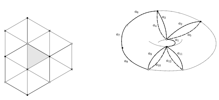
Figure 29. Doble of the annulus-diamond and its associated dessin.

The permutations associated to the dessin are

$$\sigma_{0} = (1\ 2\ 3\ 4\ 5)(9\ 8\ 10)(6\ 7)(11\ 12)$$

(46) $$\sigma_{1} = (1\ 12\ 10\ 9\ 11)(3\ 4\ 6)(2\ 5)(7\ 8).$$

Let $\omega_{0}=5-\omega$. According to Table (1) $\gamma(t)=\pi(1/2+t\omega_{0})$ factorizes in $\pi_{1}(2\Delta-\{0,1,\omega\},1/2)$, as follows

(47) $$\gamma=\gamma_{1}\gamma_{0}^{-1}\gamma_{1}^{-1}\gamma_{0}\gamma_{1}\gamma_{0}^{-1}.$$

Hence $\sigma_{\gamma}$ factorizes as

(48) $$\sigma_{\gamma}=\sigma_{0}^{-1}\sigma_{1}\sigma_{0}\sigma_{1}^{-1}\sigma_{0}^{-1}\sigma_{1}.$$

Replacing (5) in the previous equation we obtain:

(49) $$\sigma_{\gamma}=(1\ 6\ 11\ 3\ 9\ 4\ 10\ 5\ 8)(2\ 7\ 12)$$

(we used the package Sympy of Python to obtain this product).

If $\tilde{\gamma}$ is the geodesic in $X$ with tangent vector $\omega_{0}=5-\omega$ at the midpoint of the edge $a_{2}$, see Figure (30) we obtain that $\operatorname{ord}\sigma_{a_{2}}=3$ and $5-\omega\in Hex$. Hence by Corollary 7 it follows that

Figure 30. Geodesic $\tilde{\gamma}$ based at the midpoint of $a_{2}$ and with direction direccton $5-\omega$.

(50) $$\operatorname{long}\tilde{\gamma}=\operatorname{ord}\sigma_{a_{2}}|\omega_{0}|=3|5-\omega|\approx 13.76.$$

This length can be corroborated directly in Figure (30).

Analogously, if $\omega_{0}=10+\omega$, then $\sigma_{\gamma}$ has the cyclic decomposition

(51) $$\sigma_{\gamma}=(1\ 8\ 5\ 2\ 12\ 11\ 6)(3\ 4)(9\ 10)(7).$$

Hence, if $\tilde{\gamma}$ is the geodesic with tangent vector $10+\omega$ in the midpoint of $a_{7}$ (Figure (31)), one obtains:

(52) $$\operatorname{long}(\tilde{\gamma})=\operatorname{ord}\sigma_{a_{7}}|\omega_{0}|=|10+\omega|\approx 10.54.$$

Figure 31. Geodesic $\tilde{\gamma}$ based in the midpoint of $a_{1}$ with direction $10+\omega$.

If $\tilde{\gamma}$ is based in $a_{1}$, $\operatorname{ord}\sigma_{a_{1}}=7$, and

(53) $$\operatorname{long}(\tilde{\gamma})=\operatorname{ord}\sigma_{a_{1}}|\omega_{0}|=7|10+\omega|\approx 73.75.$$

The cyclic decompositions of $\sigma_{\gamma}$ in the previous examples, and others, are shown in Table (2).

Directions $\omega_{0}$	Factorization of $\sigma_{\gamma}\in S_{12}$
1. $\omega_{0}=1+\omega\in Hex$	$\sigma_{\gamma}=(1\ 12\ 2)(3\ 7\ 10\ 11\ 8\ 6\ 5)$
2. $\omega_{0}=3\omega\in Hex$	$\sigma_{\gamma}=(1\ 9\ 6\ 5\ 11\ 8\ 4)(2\ 7\ 12\ 3\ 10)$
3. $\omega_{0}=2+\omega\notin Hex$	$\sigma_{\gamma}=(2\ 4\ 11)(3\ 7\ 10)(5\ 9\ 12)$
4. $\omega_{0}=13+17\omega\in Hex$	$\sigma_{\gamma}=(1\ 5\ 12\ 7\ 2\ 11)(4\ 8\ 6\ 9)$
5. $\omega_{0}=5-\omega\in Hex$	$\sigma_{\gamma}=(1\ 6\ 11\ 3\ 9\ 4\ 10\ 5\ 8)(2\ 7\ 12)$
6. $\omega_{0}=10+\omega\in Hex$	$\sigma_{\gamma}=(1\ 8\ 5\ 2\ 12\ 11\ 6)(3\ 4)(9\ 10)$

Table 2. Some directions $\omega_{0}$ and the factorization of $\sigma_{\gamma}$ with respect to the dessin given by (5).

Proposition 15.

For each $k\geq 0$, $\omega_{0}=(3k+1)+\omega$ is contained in $Hex$. Furthermore if $\gamma_{\omega_{0}}$ is the parametrized geodesic in $2\Delta$ $t\mapsto\pi(1/2+t\omega_{0})$, then

(54) $$\gamma_{\omega_{0}}=(\gamma_{1}^{-1}\gamma_{0})(\gamma_{1}\gamma_{0}^{-1}\gamma_{1}^{-1}\gamma_{0})^{k}.$$

Therefore, if $X$ is a Riemann surface endowed with a decorated equilateral structure whose associated dessin d’enfant defines the permutations $\sigma_{0}$ and $\sigma_{1}$, then $\sigma_{\gamma}$ is factorized as follows:

(55) $$\sigma_{\gamma_{0}}=(\sigma_{0}\sigma_{1}^{-1}\sigma_{0}^{-1}\sigma_{1})^{k}\sigma_{0}\sigma_{1}^{-1}$$

Proof.

Observe that $(3k+1)+\omega=m(2-\omega)+n(1+\omega)$, with $m=k$ and $n=k+1$. This proves the first assertion.

On the other hand

(56) $$\gamma_{\omega_{0}}=\gamma_{(3(k-1)+1)+\omega}(\gamma_{1}\gamma_{0}^{-1}\gamma_{1}^{-1}\gamma_{0}).$$

Hence, if we apply the previous formula recursively we obtain

(57) $$\gamma_{\omega_{0}}=\gamma_{1+\omega}(\gamma_{1}\gamma_{0}^{-1}\gamma_{1}^{-1}\gamma_{0})^{k}.$$

Since $\gamma_{1+\omega}=\gamma_{1}^{-1}\gamma_{0}$, one has formula (54). ∎

Remark 19.

If $\sigma_{1}=(1)$ and $\omega_{0}=(3k+1)+\omega$, it follows from this proposition that $\sigma_{\gamma}=\sigma_{0}$.

Example 6.

Consider the dessin on the Riemann sphere given by Belyi’s function $z^{n}$. In this case the permutations are

$$\sigma_{0} = (1\ 2\ \cdots n)$$

(58) $$\sigma_{1} = (1).$$

Let us take the equilateral structure which turns each triangle of the triangulation defined by the dessin into an equilateral triangle. Then it follows from Remark 19 that for any geodesic $\tilde{\gamma}$ with tangent vector at some midpoint of an edge equal to $\omega_{0}=(3k+1)+\omega$ one has:

(59) $$\operatorname{long}\tilde{\gamma}=n|(3k+1)+\omega|.$$

6. Conic hyperbolic structures

6.1. Conic hyperbolic metrics on compact surfaces with a decorated triangulation.

Let $X$ be a compact surface endowed with a decorated triangulation associated to a dessin d’enfant. Then there exists a Belyi function $f_{1}\colon X\to 2\Delta$ which realizes the decorated triangulation. We recall that $\Delta$ is the equilateral triangle with vertices in $0,1$ and $\omega$, where $\omega=\exp(2\pi i/6)$; and $2\Delta$ is the sphere obtained by gluing two decorated triangles as explained at the beginning.

Let us consider a hyperbolic triangle contained in the Poincaré disk $\mathbb{D}$, which has vertices at $z_{1}$, $z_{2}$ and $z_{3}$ such that: (i) $z_{1}=0$, (ii) the edge between $z_{1}$ and $z_{2}$ is in the real axis and (iii) the triplet $(z_{1},z_{2},z_{3})$ defines a positive orientation of the triangle. Such a triangle is completely determined by its angles. If $\pi/m$, $\pi/n$ and $\pi/l$ are the angles at $z_{1}$, $z_{2}$ and $z_{3}$, respectively, then the triangle will be denoted by $\Delta_{m,n,l}$, see Figure (32). We will also suppose that the triangle is decorated with $\circ,\ \bullet$, $\ast$ in $z_{1}$, $z_{2}$ and $z_{3}$ respectively. Such a decoration determines a coloration into black and white triangles just like was done in the euclidean case.

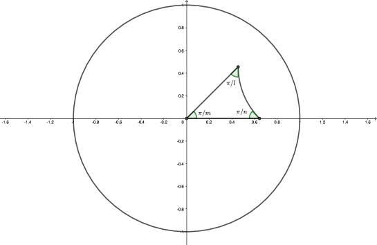
Figure 32. Hyperbolic triangle $\Delta_{m,n,l}$, with $m=n=l=4$.

By an analogous construction as that of $2\Delta$ in the euclidean case we can define $2\Delta_{m,n,l}$: we use the hyperbolic reflection $R$ which fixes, point by point, the edge between $z_{1}$ and $z_{2}$; we identify the boundary of $\Delta_{m,n,l}$ with the boundary of its reflection $R(\Delta_{m,n,l})$, using $R$. This surface $2\Delta_{m,n,l}$ is homeomorphic to the 2-sphere and it has a natural hyperbolic metric outside of the vertices. And each of the two triangles is isometric to $\Delta_{m,n,l}$. In addition, as in the euclidean case, the triangulation induces a complex structure on $2\Delta_{m,n,l}$ which turns it into a Riemann surface. We will assume that the Riemann surface $2\Delta_{m,n,l}$ is endowed with this conic hyperbolic metric.

Remark 20.

The surface $2\Delta_{m,n,l}$ is conformal to $\mathbb{H}/\Gamma_{m,n,l}$, where $\Gamma_{m,n,l}$ is the triangular group generated by $\Delta_{m,n,l}$.

There exists a conformal map which preserves the boundaries and send vertices to vertices respecting the decoration. By Schwarz Reflection Principle we can extend this map to its reflected triangles in the Poincaré disk. After identifications we have a conformal map on the quotients $\Phi\colon 2\Delta\to 2\Delta_{m,n,l}$, see Figure (33).

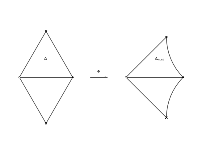
Figure 33. Conformal map between $2\Delta$ and $2\Delta_{m,n,l}$.

Using $\Phi$ we construct a Belyi function $f=\Phi\circ f_{1}\colon X\to 2\Delta_{m,n,l}$. This is a holomorphic map with respect to the complex structures we have defined. Let us notice that this function realizes the decorated triangulation we had originally.

If we pull back to $X$, using $f$, the conic hyperbolic metric of $2\Delta_{m,n,l}$, the triangles of $X$ become isometric to $\Delta_{m,n,l}$.

Summarizing, we obtain the following proposition:

Proposition 16.

Let $X$ be a surface with a decorated triangulation induced by a dessin d’enfant. For any positive integers $m,n,l$, such that $1/m+1/n+1/l<1$, there exists a conic hyperbolic metric in $X$ such that with this metric each triangle is isometric to to the hyperbolic triangle $\Delta_{m,n,l}$. This metric is induced by a Belyi function $f\colon X\to 2\Delta_{m,n,l}$ which realizes the decorated triangulation.

6.2. Representation of a Belyi function in the hyperbolic plane.

Let $X$ be a surface with a decorated triangulation $T$ induced by a dessin d’enfant. Let $O(T)$ be the greatest valence of the vertices of the triangulation $T$. If $f\colon X\to\hat{\mathbb{C}}$ is the Belyi function that realizes $T$ one has $O(T)=\max_{p\in f^{-1}\{0,1,\infty\}}\operatorname{mult}_{p}(f).$

Let $m$ be an integer, $m>3$, such that $m>O(T)$. Let us endow $X$ with the conic hyperbolic metric induced by a Belyi function $f\colon X\to 2\Delta_{m,m,m}$, which realizes the decorated triangulation (see Proposition 16).

Let $P$ be a (connected but not necessarily convex) polygon formed by a finite number of triangles of the tessellation $T(m,m,m)$ corresponding to the triangular group $\Gamma_{m,m,m}$, generated by the triangle $\Delta_{m,m,m}$ [Mag74].

Definition 4.

A hiperbolic peel of $X$ is a continuous map $\Psi\colon P\to X$ which satisfies the following conditions:

• Sends triangles of the tessellation $T(m,m,m)$ onto triangles of $T$.

• The restriction to each triangle of $T(m,m,m)$ is an isometry

• It respects the decoration (we assume that the tessellation $T(m,m,m)$ is decorated compatibly with $\Delta_{m,m,m}$).

• The function is injective in the interior of $P$ and each point of $X$ has at most two pre-images bajo $\Psi$. Thus the double pre-images can occur only at $\partial{P}$, the boundary of $P$.

If we define the equivalence relation in $P$ as $x\sim y$ if and only $\Psi(x)=\Psi(y)$, we obtain a rule to glue some sides of the boundary of the polygon by hyperbolic isometries that belong to the triangle group $\Gamma_{m,m,m}$. Condition (iv) implies that an edge on the boundary is paired with at most another edge, but it is possible that certain edges are not paired with any other edge.

Note that the peel $\Psi$ descends to the quotient to an embedding $\hat{\Psi}\colon(P/_{\sim})\to X$.

Example 7.

Figure (34) shows the peel which corresponds to the elliptic curve from Figure (35). The function $\Psi$ maps each triangle onto $\Delta_{i}$ in $T_{i}$ respecting the decorations. Here, as before, we assume that the hexagon has the metric induced by the Belyi function $f\colon X\to 2\Delta_{4,4,4}$.

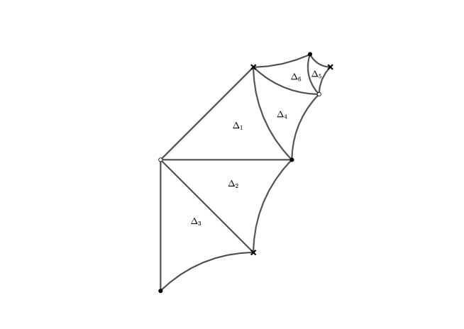
Figure 34. Peel associated to the elliptic curve $\mathbb{C}/\Lambda_{1,\omega}$, with $\omega=\exp(2\pi i/6)$. In this case we take $m$ equal to $4$.

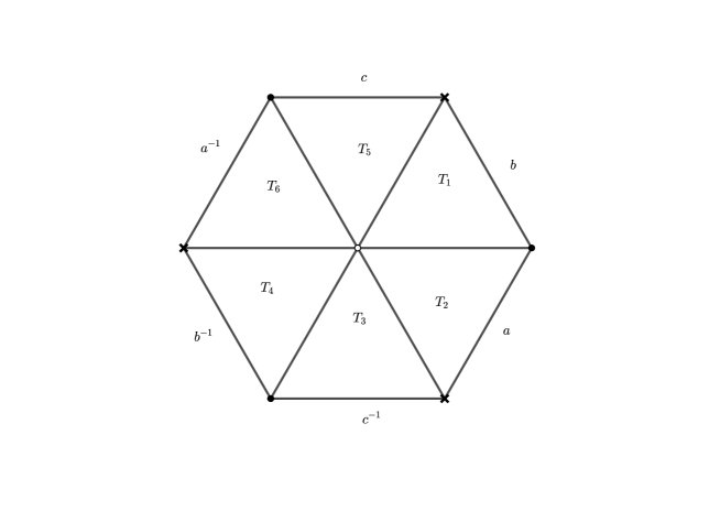
Figure 35. Hexagon with sides identified, corresponding to $\mathbb{C}/\Lambda_{1,\omega}$, with $\omega=\exp(2\pi i/6)$.

Remark 21.

Each vertex $p$ of the polygon $P$ belongs to at most $O(T)$ triangles of $P$; since $m>O(T)$, the union of such triangles is not a neighborhood of $p$. Therefore all the vertices of the triangulation of $P$ are in its boundary $\partial{P}$.

Remark 22.

If all of the edges of $\partial{P}$ are pairwise identified then $\hat{\Psi}$ is surjective, hence it is a homeomorphism because $\Psi(P/_{\sim})$ is a connected surface without boundary contained in $X$.

Proposition 17.

If one of the edges of $\partial{P}$ is not paired with some other edge then $\Psi$ can be extended to a polygon with one more triangle than the number of triangles of $P$.

Proof.

Let $a$ be an edge of $\partial{P}$ which is not paired with any other edge. Let us add to $P$ the triangle $\Delta_{1}$, of the tessellation, which has $a$ as an edge and which does not belong to $P$. Such triangle must exist because $a$ is in the boundary of $P$. Since $m>O(T)$ the edges of $\Delta_{1}$, which are distinct to $a$, are not in $P$; this insures us that we don’t use edges which are paired with other edges of $\partial{P}$.

One decorates the vertices of the added triangle $\Delta_{1}$ according to the edge $a$ and color it according to the positive or negative orientation determined by the ordering of the vertices.

If $T_{1}$ is the triangle in $X$, adjacent to $\Psi(a)$, define $\Psi\colon\Delta_{1}\to T_{1}$ as the isometry which preserves the decoration we obtain a peel $\Psi\colon P\cup\Delta_{1}\to\Psi(P)\cup T_{1}$ that has one more triangle than $P$. ∎

Remark 23.

It follows from Proposition 17 and by an argument of maximality, since the triangulation has a finite number of triangles, that there exist a peel $\Psi\colon P\to X$ such that every edge in $\partial{P}$ is paired with another edge so that the edge of the boundary are pairwise identified. Then, by Proposition 22, $\Psi$ descends to a homomorphism $\hat{\Psi}\colon(P/_{\sim})\to X$ which is a conformal map.

Summarizing we have the following theorem:

Theorem 7.

If $X$ is a decorated surface with a conic hyperbolic metric induced by a Belyi function $f\colon X\to 2\Delta_{m,m,m}$ which realizes the triangulation, and $m$ is integer such that $m>3$ and $m>O(T)$. Then there is a peel $\Psi\colon P\to X$ which is maximal and which descends to a conformal mapping to the quotient $\hat{\Psi}\colon(P/_{\sim})\to X$.

$\hat{\Psi}\colon(P/_{\sim})\to X$ is a conformal map which sends triangles onto triangles of the respective triangulations. It also respect the decorations and it restriction to each triangle is an isometry. Also $P/_{\sim}$ has Belyi function $f_{P}\colon(P/_{\sim})\to 2\Delta_{m,m,m}$, defined as the map which sends triangles onto triangles, by an isometry which respects the decorations, including the colorations of the triangles. By construction, the map $\hat{\Psi}$ is an isomorphism of ramified coverings i.e, the following diagram commutes:

(60)

6.3. The case of ideal decorated hyperbolic triangulations

In the same fashion as in the case of hyperbolic triangles $\Delta_{m,n,l}$ with positive angles $\pi/m$, $\pi/n$ and $\pi/l$ we can consider the case when the triangle is ideal i.e, its angles are all equal to 0 ($m=n=l=\infty$).

In particular we consider the ideal triangle in the upper half plane $\mathbb{H}$ that has as its vertices $0$, $1$ and $\infty$. We denote this triangle by $\Delta_{\infty,\infty,\infty}$, see Figure (36).

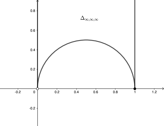
Figure 36. Ideal triangle with vertices in $0$, $1$ and $\infty$.

The vertices $0$, $1$ and $\infty$ are decorated with the symbols $\circ,\bullet,\ast$ respectively; then we use the hyperbolic reflection $R$ with respect to the edge which connects $\circ$ with $\bullet$, and we identify the boundary of $\Delta_{\infty,\infty,\infty}$ with the boundary of $R(\Delta_{\infty,\infty,\infty})$ by the reflection $R$.

The surface of genus 0 constructed as the union along the boundary of two ideal triangles has a complete hyperbolic metric and therefore the metric induces a complex structure. As a Riemann surface it is conformally equivalent to the Riemann sphere minus three points. This decorated surface will be denoted by $2\Delta_{\infty,\infty,\infty}$.

Remark 24.

The surfsce $2\Delta_{\infty,\infty,\infty}$ is also conformally equivalent to $\mathbb{H}/\Gamma(2)$ where the group $\Gamma(2)$ is the modulo 2 congruence subgroup of $\text{PSL}(2,\mathbb{Z})$ (we recall that $\Gamma(2)=\Gamma_{\infty,\infty,\infty}$).

If $X$ is a decorated triangulated surface, obtained from a dessin d’enfant, there exists a Belyi map $f\colon X\to 2\Delta_{\infty,\infty,\infty}$ which realizes the decorated triangulation. Therefore we can endow $X$ with a conic hyperbolic metric by pulling-back the conic hyperbolic metric of $2\Delta_{\infty,\infty,\infty}$, by means of $f$.

Also in this case one has a maximal peel, $\Psi\colon P\to X$, which descends to the quotient to a conformal map $\hat{\Psi}\colon(P/_{\sim})\to X$. The definition of the peel is completely analogous to the case of finite triangles.

The following remark highlights the advantage of using ideal triangles:

Remark 25.

In this case as $P$ is an ideal polygon it must be convex.

The ideal peel of $P$ can also be obtained from the uniformization of the sphere with three punctures: we consider $2\Delta_{\infty,\infty,\infty}$ as the quotient $\mathbb{H}/\Gamma(2)$. If $f\colon X\to\mathbb{H}/\Gamma(2)$ is a Belyi function, by properties of covering spaces there is a subgroup $K_{0}$ of of finite index of $\Gamma(2)$ and a conformal map $\Psi$ such that the following diagram is commutative:

(61)

where $\pi$ is the function which acts on right cosets as follows: $[z]_{K_{0}}\mapsto[z]_{\Gamma(2)}$. Then, $\Psi$ must send triangles onto triangles, preserve the decoration and be an isometry when restricted to each triangle. Therefore if we consider a fundamental domain $P$ of the action of $K_{0}$, we obtain a peel $\Psi\colon P\to X$ which coincides, in the quotient, with the map $\Psi$ in Diagram (61).

Example 8.

In Figure (37) we show three parallelograms identified along their boundaries (as indicated in the figure). The surface with boundary obtained after gluing is a closed annulus. Such an annulus is decorated as indicated in the figure. If we take the double of this annulus we have a surface $X$, with a decorated triangulation and homeomorphic to the 2-torus.

In Figure (37) we label the triangles with the symbols $\Delta_{i}$, $i=1,2,3,4,5,6$. In addition, we suppose that the triangles in the other part of the double are labeled in $X$ with the symbols $\Delta_{i}^{\prime}$, $i=1,2,3,4,5,6$, in such a way that $\Delta_{i}^{\prime}$ is the double of $\Delta_{i}$.

We chose the (unique) conic hyperbolic metric on $X$ which renders each triangle $\Delta_{i}$ and $\Delta_{i}^{\prime}$ isometric to the ideal hyperbolic triangle with vertices in $1,\rho,\rho^{2}$, where $\rho=\exp(2\pi i/3)$. We also suppose that the vertices have the original decoration.

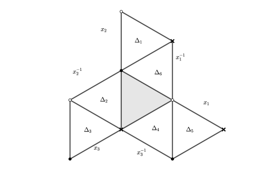
Figure 37. Parallelograms identified along their boundaries. The sides marked with letters are identified according to the orientation. After the identification one gets an annulus.

Let $P$ be the ideal decorated polygon in Figure (38). Define $\Psi\colon P\to X$ as the function which maps each triangle of $P$ (Figure (38)) onto a triangle of $X$ by an isometry which preserves the decoration and according with the labels. By definition $\Psi$ es a peel of $X$.

We observe that $\Psi(\partial P)$ is a graph in the surface and it is a union of edges of the triangulation. (Figure (39)).

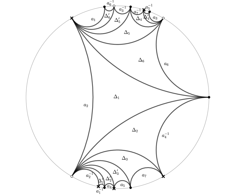
Figure 38. Example of an ideal peel. If we identify the edges of the boundary as indicated in the figure we get an elliptic curve.

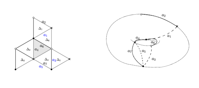
Figure 39. The image of $\partial P$ under $\Psi$ is a graph in $X$ such that ita complement in $X$ is simply connected. In the right-hand-side of the picture the letters in blue indicates that the edge is in the reverse of the triangle.

Definition 5.

Let $X$ be a Riemann surface and $\Gamma$ a subgroup of $\operatorname{Aut}(X)$ (the group of holomorphic automorphisms of $X$). We say that a region $F$ of $X$ is a fundamental domain of $\Gamma$ if: i) any $z\in X$ is equivalent (i.e, is in the same orbit) under the action of $\Gamma$ with an element $z^{\prime}$ in the closure of $F$, ii) two distinct points in $F$ are not equivalent under the action of $\Gamma$.

Remark 26.

Let us suppose that $X$ is an elliptic curve (i.e, a compact Riemann surface of genus 1). Suppose that the complex structure is given by an equilateral decorated hyperbolic triangulation with triangles isometric to $\Delta_{\infty,\infty,\infty}$.

Let $\Psi\colon P\to X$ be an ideal peel for $X$. Suppose that $\Lambda_{1,\tau}=\left\{m+n\tau\,\,:\,m,n\in\mathbb{Z}\right\}$ is the lattice which uniformizes $X$ i.e, $X\cong\mathbb{C}/\Lambda_{1,\tau}$ and $\pi\colon\mathbb{C}\to X$ is the universal covering map such that $\operatorname{Deck}(\pi)$ (the group of deck transformations) is equal to $\Lambda_{1,\tau}$.

Since $P$ is simply connected by covering space theory, we can find a lifting of $\Psi$ to a map from $P$ to $C$ i.e, a map $\tilde{\Psi}$ such that the diagram (62) is commutative:

(62)

Wr claim that $\tilde{\Psi}(\mathring{P})$ is a fundamental domain for $\Lambda_{1,\tau}$, where $\mathring{P}$ denotes the interior of $P$. This is equivalent to proving that $\pi(\overline{\tilde{\Psi}(\mathring{P})})=X$ and that $\pi\colon\tilde{\Psi}(\mathring{P})\to X$ is injective. To prove the first assertion, note that by continuity $\overline{\tilde{\Psi}(\mathring{P})}=\tilde{\Psi}(P)$, hence

(63) $$\pi(\overline{\tilde{\Psi}(\mathring{P})})=\pi(\tilde{\Psi}(P))=\Psi(P)=X.$$

To prove the second assertion, let $x,y\in\tilde{\Psi}(\mathring{P})$ be such that $\pi(x)=\pi(y)$. Then, there exist $p_{1},p_{2}\in\mathring{P}$ such that $x=\tilde{\Psi}(p_{1})$ and $y=\tilde{\Psi}(p_{2})$. Since the diagram (62) commutes $\Psi(p_{1})=\Psi(p_{2})$, hence $p_{1}=p_{2}$ hence $x=y$. This proves that $\tilde{\Psi}(\mathring{P})$ is a fundamental domain for $\Lambda_{1,\tau}$.

7. Peels of a decorated equilateral triangulation of an elliptic curve and its modulus $\tau$

Remark 27.

Let $X$ be a Riemann surface obtained from a decorated equilateral triangulation. We have a decorated graph whose edges and vertices are the edges and vertices of the triangulation. If $\Psi\colon P\to X$ is a peel for $X$, then $\mathcal{G}_{P}$ will denote the subgraph $\Psi(\partial P)$. In Figure (39) (right-hand-side of the picture) we can see the graph $\mathcal{G}_{P}$ for the peel shown in (Figure (38)).

Recall that two topological spaces $X$ and $Y$ have the same homotopy type if there exist maps $f\colon X\to Y$ and $g\colon Y\to X$ such that $g\circ f$ is homotopic to the identity map $id_{X}$ and $f\circ g$ is homotopic to $id_{Y}$.

Two connected graphs (finite or not) have the same homotopy type if and only if their fundamental group (which are free groups) are isomorphic.

Proposition 18.

Let us suppose that $X$ is an elliptic curve obtained from a decorated equilateral triangulation. If $\Psi\colon P\to X$ is a peel for $X$. Then $\mathcal{G_{P}}$ is homotopic to a bouquet of two circles. Hence, $\pi_{1}(\partial\mathcal{G}_{P},x_{0})$ is a free group in two generators for any $x_{0}$ in $\partial\mathcal{G}_{P}$.

Proof.

By graph theory, the graph $\mathcal{G}_{P}$ has the homotopy type of a bouquet of the following number of circles:

(64) $$\beta_{1}(\mathcal{G}_{P})=1-\chi(\mathcal{G}_{P})=1-v+a$$

where $\chi(\mathcal{G}_{P}$) is the Euler characteristic of the graph. One has the cell decomposition of the torus $X$ given by the vertices and edges of $\mathcal{G}_{P}$ and the unique 2-cell which is the complement of the graph on the torus (the interior of $P$ is the unique 2-cell) we have that $\chi(X)=0=v-a+1$, hence $1-\chi(\mathcal{G}_{P})=2$. ∎

Remark 28.

The same proof can be used to show that, if instead of the torus, $X$ is a surface of genus $g$ then $1-\chi(\mathcal{G}_{P})=2g$ so $\mathcal{G}_{P}$ and the first Betti number of $\mathcal{G}_{P}$ is $2g$ so that it is homotopic to a bouquet of $2g$ circles.

Remark 29.

Let us suppose that $X$ is an elliptic curve obtained from a decorated equilateral triangulation. Then if $\Psi\colon P\to X$ is a peel for $X$.

From the homology long exact sequence of the pair $(X,\mathcal{G}_{P})$, since $X-\mathcal{G}_{P}$ is contractible, it follows that the inclusion $i\colon\mathcal{G}_{P}\to X$ induces an isomorphism in the first homology groups:

(65) $$i_{*}\colon H_{1}(\mathcal{G}_{P},\mathbb{Z})\to H_{1}(X,\mathbb{Z}).$$

Hence,

(66) $$i_{\#}\colon\pi_{1}(\mathcal{G}_{P},x_{0})\to\pi_{1}(X,x_{0})$$

is an epimorphism from the free group in two generators onto the fundamental group of the elliptic curve which is isomorphic to $\mathbb{Z}\oplus\mathbb{Z}$. Therefore we can choose two curves $\gamma_{1}$ and $\gamma_{2}$ based at a point $x_{0}\in\mathcal{G}_{P}$, totally contained in $\mathcal{G}_{P}$, and which generate $\pi_{1}(X,x_{0})$.

Remark 30.

Let $X$ be a Riemann surface with a marked base point $x_{0}$ and $p\colon(\tilde{X},\tilde{x}_{0})\to(X,x_{0})$ be its universal covering, with $\tilde{x}_{0}\in\tilde{X}$ in the fiber of $x_{0}$. By the theory of covering spaces it follows that for each $[\gamma]\in\pi_{1}(X,x_{0})$ there exists a unique $g_{\gamma}\in\operatorname{Deck}(\tilde{X},p)$ such that $g_{\gamma}(\tilde{x}_{0})=\tilde{\gamma}(1)$, where $\tilde{\gamma}$ is the lifting of $\gamma$ based in $\tilde{x}_{0}$. Hence, we have a function $\pi_{1}(X,x_{0})\to\operatorname{Deck}(\tilde{X},p)$. It can be shown that this funcion is a group isomorphism.

Therefore one has the following theorem:

Theorem 8.

Suppose that $X$ is an elliptic curve obtained by a decorated equilateral triangulation. Let $p\colon\mathbb{C}\to X$ be its holomorphic universal covering. If $\Phi\colon P\to X$ is a hyperbolic peel for $X$, the there exist two curves $\gamma_{1}$ and $\gamma_{2}$ en $\mathcal{G}_{P}$ such that $g_{\gamma_{1}}(z)=z+\omega_{1}$ and $g_{\gamma_{2}}(z)=z+\omega_{2}$ generate $\operatorname{Deck}(p)$. Hence: $\tau=\omega_{1}/\omega_{2}$ uniformize to $X$ i.e, $X$ has modulus $\tau$ and $X$ is biholomorphic to $\mathbb{C}/\Lambda_{1,\tau}$.

8. Final remarks and questions

The complex structures of surfaces $X$ deduced by a dessin $\mathcal{D}$ depend only on the combinatorics of the triangulation $T_{\mathcal{D}}$ induced by the dessin or, equivalently, on the branched covering given by the associated Belyi map $f_{\mathcal{D}}:X\to\hat{\mathbb{C}}$. This in turn is given by a representation $\rho_{\mathcal{D}}:\pi_{1}(\bar{\mathbb{C}}-\{0,1,\infty\})\to{S_{n}}$ from the fundamental group of $\bar{\mathbb{C}}-\{0,1,\infty\}$ (which is a nonabelian free group in two generators) into the symmetric group $S_{n}$ of permutations of $n$ objects. So we have the quadruple $(\mathcal{D},T_{\mathcal{D}},f_{\mathcal{D}},\rho_{\mathcal{D}})$ where each entity determines completely the other three.

In all that follows $X$ will be an elliptic curve obtained from a decorated equilateral triangulation induced by a dessin d’enfant $\mathcal{D}$. Suppose that $\mathcal{D}$ determines a Belyi function with 3 critical values (and not less than 3) which we always assume are 0, 1 and $\infty$. Then $\mathcal{D}$ determines a decorated equilateral triangulation $T_{\mathcal{D}}$ by isometric equilateral triangles which are either euclidean or hyperbolic.

there are several interesting questions

1. What properties must satisfy $\mathcal{D}$ (equivalently the combinatorics of $T_{\mathcal{D}}$ or $\rho_{\mathcal{D}}$) so that the elliptic curve is defined over $\mathbb{Q}$?

2. What properties must satisfy $\mathcal{D}$ (equivalently the combinatorics of $T_{\mathcal{D}}$ or $\rho_{\mathcal{D}}$) so that the elliptic curve is modular?

3. What properties must satisfy $\mathcal{D}$ so that the elliptic curve is defined over a quadratic extension $\mathbb{Q}(\sqrt{d})$ (for $d\in\mathbb{Z}$ not divisible by a square)? In particular, what are the properties for $\mathcal{D}$ for $X$ to be an elliptic curve with complex multiplication? (partial results about this question are described in [JW16] section 10.2).

We remark that if for an elliptic curve the conditions in item 1) imply the conditions in item 2), this would prove the celebrated Taniyama-Shimura conjecture, which in now a theorem. In 1995, Andrew Wiles and Richard Taylor [Wil95, TW] proved a special case which was enough for Andrew Wiles to finally prove Fermat’s Last Theorem. In 2001 the full conjecture was proven by Christophe Breuil, Brian Conrad, Fred Diamond and Richard Taylor [BCDT]. This was one of the greatest achievements in the field of mathematics of the last quarter of the XX century.

To prove that for an elliptic curve the conditions in 1) imply the conditions in 2) is the Jugentraum of the first author (JJZ) and the Alterstraum of the second (AV)!

References

- [Bel79] G. V. Belyi, Galois extensions of a maximal cyclotomic field, Izv. Akad. Nauk SSSR Ser. Mat. 43(2) 267–276, 479 (1979).
- [BCDT] Breuil C.; Conrad B.; Diamond F.; Taylor, R., On the modularity of elliptic curves over : Wild 3-adic exercises, Journal of the American Mathematical Society 14 (2001), pp. 843–939
- [Bost] Bost, J-B. Introduction to Compact Riemann Surfaces, Jacobians and Abelian Varieties From number theory to physics (Les Houches, 1989), 64–211, Springer, Berlin, 1992.
- [BNN95] Brunet, R.; Nakamoto, A. ; Negami, S. Diagonal flips of triangulations on closed surfaces preserving specified properties. J. Combin. Theory Ser. B 68 (1996), no. 2, 295–309.
- [CoItzWo94] Cohen, Paula Beazley; Itzykson, Claude; Wolfart, Jürgen Fuchsian triangle groups and Grothendieck dessins. Variations on a theme of Belyǐ. Comm. Math. Phys. 163 (1994), no. 3, 605–627.
- [Esquisse] Grothendieck, A.; Esquisse d’un programme. In L. Schneps & P. Lochak (Eds.), Geometric Galois Actions (London Mathematical Society Lecture Note Series, pp. I-Vi). Cambridge: Cambridge University Press (1997).
- [For81] Forster O., Lectures on Riemann surfaces, Graduate Texts in Mathematics, 81, Springer-Verlag (1981).
- [GG12] Girondo E. & González-Diez G., Introduction to compact Riemann surfaces and dessins d’enfants, London Mathematical Society Student Texts, 79, Cambridge University Press (2012).
- [Gui14] Guillot, P. An elementary approach to dessins d’enfants and the Grothendieck-Teichml̈ler group. Enseign. Math. 60 (2014), no. 3-4, 293–375.
- [JW16] Jones,G. A.; Wolfart, J. Dessins d’enfants on Riemann surfaces. Springer Monographs in Mathematics. Springer, Cham, 2016. xiv+259 pp.
- [Mag74] Magnus, W., Noneuclidean tesselations and their groups. Pure and Applied Mathematics, Vol. 61. Academic Press [A subsidiary of Harcourt Brace Jovanovich, Publishers], New York-London, 1974. xiv+207 pp.
- [ShVo90] Shabat, G. B.; Voevodsky, V. A. Drawing curves osee number fields. The Grothendieck Festschrift, Vol. III, 199–227, Progr. Math., 88, Birkhäuser Boston, Boston, MA, 1990.
- [ShZv94] Shabat, G. B.; Zvonkin, A.Plane trees and algebraic numbers. Jerusalem combinatorics 93, 233–275, Contemp. Math., 178, Amer. Math. Soc., Providence, RI, 1994.
- [Spr81] Springer G., Introduction to Riemann surfaces, 2nd ed. (1981).
- [TW] Taylor, R,; Wiles, A., Ring-theoretic properties of certain Hecke algebras. Ann. of Math. (2) 141 (1995), no. 3, 553–572
- [Troy07] Troyanov, M. On the moduli space of singular euclidean surfaces Handbook of Teichml̈ler theory. Vol. I, 507–540, IRMA Lect. Math. Theor. Phys., 11, Eur. Math. Soc., Zürich, 2007.
- [VSh89] Voevodskiǐ, V. A.; Shabat, G. B. Equilateral triangulations of Riemann surfaces, and curves over algebraic number fields. (Russian) Dokl. Akad. Nauk SSSR 304 (1989), no. 2, 265–268; translation in Soviet Math. Dokl. 39 (1989), no. 1, 38–41.
- [Wil95] Wiles, A., Modular elliptic curves and Fermat’s last theorem. Ann. of Math. (2) 141 (1995), no. 3, 443–551