A Non-Intrusive Correction Algorithm for Classification Problems with Corrupted Data
Abstract
A novel correction algorithm is proposed for multi-class classification problems with corrupted training data. The algorithm is non-intrusive, in the sense that it post-processes a trained classification model by adding a correction procedure to the model prediction. The correction procedure can be coupled with any approximators, such as logistic regression, neural networks of various architectures, etc. When training dataset is sufficiently large, we prove that the corrected models deliver correct classification results as if there is no corruption in the training data. For datasets of finite size, the corrected models produce significantly better recovery results, compared to the models without the correction algorithm. All of the theoretical findings in the paper are verified by our numerical examples.
keywords:
Data corruption, deep neural network, cross-entropy, label corruption, robust loss1 Introduction
Classification problems arise in many practical applications, such as image classification, speech recognition, spam filtering, and so on. Over the past decades, classification has been widely studied by using machine learning techniques, which seek to learn a classifier from labeled training dataset to predict class labels for new data. However, real-world datasets often contain noise and their class labels can be corrupted, i.e., mislabelled. This can be caused by a variety of reasons, including human error, measurement error, or subjective bias by labelers, etc. Label corruptions also occur in data poisoning [16, 30]. For a more comprehensive review of the sources of label corruptions, see Section B of [4]. Label corruptions, natural or malicious, can adversely impact classification performance of classifiers. See, for example, [36, 38, 26] for impacts on different machine learning techniques. It is therefore important to explore robust techniques that can mitigate, or even eliminate, the consequences of label corruptions.
1.1 Related work
There exist a large amount of literature on learning of classifiers in the presence of label noises/errors. See, for example, [4] for a detailed survey. Methods to enhance model robustness against label noises include modifying network architecture and introducing corrections to loss function [14, 28, 10]. Larsen et al. [14] proposed a framework for designing robust neural network classifiers by introducing a probabilistic model for corruptions. Mnih and Hinton [23] introduced two robust loss functions to deal with incomplete or poorly registered labels for binary classification of aerial images. In [31], Sukhbaatar et al. suggested introduction of a noise layer into neural network models to adapt the network outputs to match the noisy label distribution. The parameters of the noise layer was estimated as part of the training process and involved modifications to current training infrastructures for deep network [31]. Later, Patrini et al. [28] developed two procedures for loss function correction, based on transition matrix measuring the probabilities of each class being corrupted into another. They also proposed an estimate of those probabilities [28], by extending the noise estimation technique in [22] to multi-class setting. The readers are also referred to [35, 33, 17, 10] for more studies on label noise robustness and loss correction techniques under the assumption that one has access to a small subset of clean data during training.
Efforts were also made to design inherently noise-tolerating (also called noise-robust) algorithms or loss functions. For binary classification, it was proved that 0-1 loss is robust to symmetric or uniform label noises, while most of the standard convex loss functions are not [19, 20]. Several theoretically motivated noise-tolerating loss functions, including ramp loss, unhinged loss and savage loss, have been introduced in the context of support vector machines (cf. [2, 32, 21]). For binary classification, Natarajan et al. [25] proposed an approach to modify any given surrogate loss function to achieve noise robustness. In the context of deep neural networks, Ghosh et al. [6, 5] derived sufficient conditions for loss function to be robust against label corruptions for binary classification [6] and multi-class classification [5]. Recently, Zhang and Sabuncu [37] generalized the commonly-used categorical cross entropy (CCE) loss to a set of noise-robust loss functions, which includes mean absolute error (MAE) loss as a special case. Other techniques that address various aspects of learning with noisy labels. They include, but are not limited to, cleaning up noisy labels [33, 27], directly modelling the label noise and then using the expectation-maximization algorithm to learn the distribution of the true labels [35, 12], and reweighting the samples according to the confidence in them [18, 29, 11].
1.2 Contributions of the present paper
The focus of this paper is on a novel correction algorithm for multi-class classification problems with corrupted training data. A distinct feature of our algorithm is that the correction procedure is applied to the output of a pre-trained model. That is, it does not require modification to a particular model training method and is performed only after the completion of the model training. Therefore, our correction method is non-intrusive and highly flexible for practical computations. The non-intrusive feature is not available for many of the aforementioned existing techniques (cf. [14, 23, 31, 28, 10]), most of which require modification to the model training architecture and/or loss function. The proposed correction procedure in this paper, on the other hand, can be readily coupled with any existing classification methods, such as logistic regression or deep neural network learning, provided that categorical cross entropy (CCE) loss or squared error (SE) loss is employed. The proposed correction algorithm is based upon our theoretical analysis for classification problems with corrupted dataset. We prove that, for sufficiently large dataset, the impact of corruption errors is minimal. More precisely, upon applying the proposed correction algorithm, the classification results become exact, as if there is no data correction, when the size of dataset approaches infinity. We also derive conditions, under which the original model without using the correction algorithm becomes inherently robust against label corruptions. Moreover, if the probability of mis-classification is uniform, we prove that the classification results are always correct in the limit of infinitely large dataset, provided that a (small) portion of clean data exists in the dataset. Numerical examples are provided to confirm the theoretical analysis and demonstrate the performance of the proposed correction algorithm.
This paper is organized as follows. After the basic problem setup in Section 2, we present some theoretical analysis on classification problem with corrupted labels in Section 3. Based on the analysis, our non-intrusive correction algorithm is then presented in Section 4.1. Extensions of the analysis and algorithm to more general cases are presented in Section 4.2. In Section 5, we present an extensive set of numerical examples, including well known benchmark problems using real-word datasets, to verify the theoretical findings and demonstrate the effectiveness of the proposed correction algorithms.
2 Problem Setup
Let be non-overlapping regions in with for . A feature set is defined to be and equipped with a probability measure . Each feature is associated with a label . We use one-hot encoding for the label, i.e., if , where is -vector with value in its th component and otherwise. Let denote the label set.
We are given a sample set , which are i.i.d. drawn from . For each sample , let be its observed label, which may be corrupted and different from the true label . We assume a subset of the labels are corrupted and denote its proportion to the entire dataset as , i.e., . For each sample , we assume its observed label is a realization of a random variable with distribution
| (1) |
where and . We assume that the corruption ratio and the distribution are available (or can be reliably estimated). However, no prior information is available about the corrupted subset .
Let be the probability simplex, where is the probability of a feature to be in . We seek to learn a probability function and define a classifier
| (2) |
If maximum probability is attained by multiple labels, we define the first one as the predicted classifier. The classification completely recovered, if for any , we have . That is, the classification is able to correctly produce the true classification.
We employ neural networks to train the classifier via minimizing the following empirical risk
| (3) |
where denotes the model parameters in the network and is the loss function. We are interested in the commonly used categorical cross-entroy (CCE) and squared-error (SE) loss functions, defined as
| (4) |
Let be the network parameters upon satisfactory training and be the trained model.
3 Main Theoretical Analysis
In this subsection, we present theoretical analysis for the above classification problem. We first derive conditions on the corruption ratio and the distribution , under which the CCE and the SE loss functions are inherently robust against the label corruption. Based upon the analysis, we propose a modified classifier, to be used after data training, to eliminate the impact of corrupted data.
3.1 Asymptotic Empirical Risk
Most of analysis is based on the assumption that the data set is sufficiently large, i.e., . Let , . The empirical risk (3) can be split into parts as
When, the following approximation holds:
where . Note that for all , the label is a realization of the random variable with the distribution (1). When , the summation in can be considered as approximation to expectation,
| (5) |
Therefore, when , we have
| (6) |
As the number of data , the empirical risk approaches . Subsequently, we call asymptotic empirical risk.
3.2 Main Results
Our main theoretical results are summarized as follows.
Theorem 1.
Remark 3.1.
Theorem 1 implies that the classification is completely recovered if and only if
| (8) |
or equivalently,
| (9) |
In other words, under the condition (9), it holds for all .
Remark 3.2.
Since for any , a direct consequence of the condition (9) is that when , the classification can always be completely recoverred, given any corruption distribution .
As a direct consequence of the above theorem, we have the following results for two special cases.
Corollary 2.
3.3 Post-Modified Classifier
The analysis in the previous section suggests a way to modify the trained classifier, so that the classification can become completely recovered, even if label corruptions do not satisfy the condition (9). We refer this as post-modified classifier, because it can be applied after the training is completed.
When the corruption probability and proportion are known, via certain estimation procedure such as [31, 28, 10], we propose to use the following modified classification function:
| (14) |
where minimizes the asymptotic empirical risk (6) and is constant vector
| (15) |
As a direct consequence of Theorem 1, we have the following conclusion.
Theorem 4.
Theorem 4 indicates that the modified classifier can completely recover the exact classification for any and any .
4 Implementation and Extension
4.1 Implementation Algorithm
In this section, we discuss implementation detail of the aforementioned classification method. Note that the theoretical analysis in the previous section does not depend on the type of approximation for – it can be linear regression, nonlinear neural networks, etc. Our discussion here is in the context of neural network (NN), because it is the predominant methods used for classification problems, see, for example, [7, 9].
Assume we are given a sample set , the corresponding observed labels , the corruption ratio and the corruption distribution . As illustrated in Fig. 1, the implementation of our algorithm is outlined as follows.
- Step 1
-
Construct a neural network (NN) with as input to approximate the probability function. Let be the operator of the NN, where is the parameter set including all the parameters in the network. To ensure the output always belongs to the probability simplex , we exploit the standard softmax function , defined by
in the output layer of the network.
- Step 2
- Step 3
-
Employ the non-intrusive post-correction (14)
- Step 4
-
Build the final classifier by argmax procedure:
(17)
A graph illustrating the steps is in Figure 1.
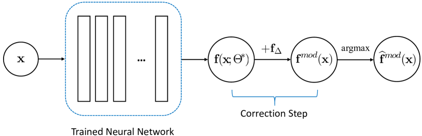
Note that Step 3 and Step 4 are applied only after the network training has been completed. Therefore, they are “non-intrusive” and do not require modification to the NN structure or training. These steps can be applied to any suitable NN for classification problems.
4.2 Extension
Our main theoretical results from Section 3 can be extended to a more general setting, by extending the basic assumption of the corruption probability (1) More specifically, we assume that, for each sample , its observed label is a realization of a random variable with the distribution
| (18) |
This is the probability that the label is corrupted to and satisfies the obvious condition
Let be the corruption probability matrix. and we have the following result, as an extension of Theorem 1.
Theorem 5.
Proof.
The proof is similar to the proof of Theorem 1 and is omitted. ∎
Suppose the corruption probability matrix and corruption proportion are known, via statistical estimation procedures such as those in [31, 28, 10], and matrix is nonsingular, we propose the following new modified classification function
This modified classification function can completely recover the exact classification for any and any transition matrix satisfying .
5 Numerical Examples
In this section, we present numerical examples. We first present two well studied academic examples to verify the theoretical results in Section 3. We then present two practical examples using well known existing datasets to demonstrate the applicability of the proposed algorithm on practical classification problems. In all examples, we test both the CCE and the SE loss functions (4). Neural network training and cost minimization problems are solved with the Adam algorithm [13] with the parameters set as in the Algorithm 1 of [13]. All the examples are implemented with the open-source libraries Keras [3] and Tensorflow [1].
Example 1: Binary Classification
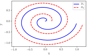
We first consider a binary classification problem from the Swiss Roll example [8]. The feature set consists of two spirals, as in Fig. 2, in the following form
| (19) |
where . The training samples are obtained by sampling the parameter according to the uniform distribution over . To verify the theories in in Section 3 for sufficiently large datasets, we use two million samples, with one million for each class. The labels are then corrupted with a fixed corruption ratio .
The classifier is constructed by employing a feedforward neural network with hidden layers and each layer contains neurons. We use the rectified linear unit (ReLU) [24] activation function in the hidden layer and the softmax activation function in the output layer.
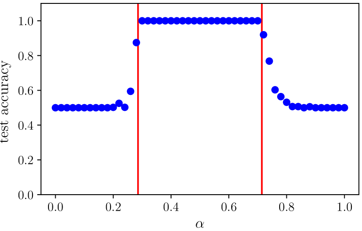
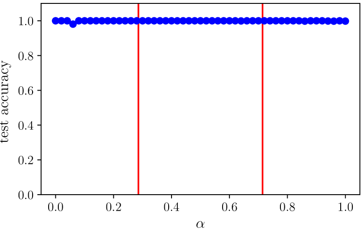
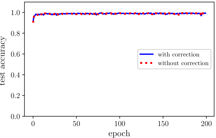
We first verify the theoretical condition (11) for the complete recovery for binary classification problems. To this end, we take the corruption probability for . For each value of we corrupt the labels and train the neural network for a sufficiently large number of epochs such that the training loss and the test accuracy attain a steady state. The accuracy is tested on a separate clean test data set of size . We present the test accuracy for different values of in Fig. 3. To show the effectiveness of the correction algorithm, we present the accuracy plot generated by the classifier without the correction step as well. For the corruption ratio , the classification can be fully recovered if , based on (11). This inverval is indicated by two red vertical lines in Fig. 3 We clearly observe that when the corruption parameter and satisfy the condition (11), the classification can be fully recovered with test accuracy almost . Otherwise, the test accuracy stays at around , no matter how sufficient the training is. Once our proposed correction algorithm is applied, the classification is fully recovered for any value of . This verifies the theoretical results in Corollary 2 and the effectiveness of the correction algorithm.

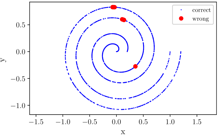
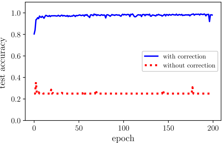
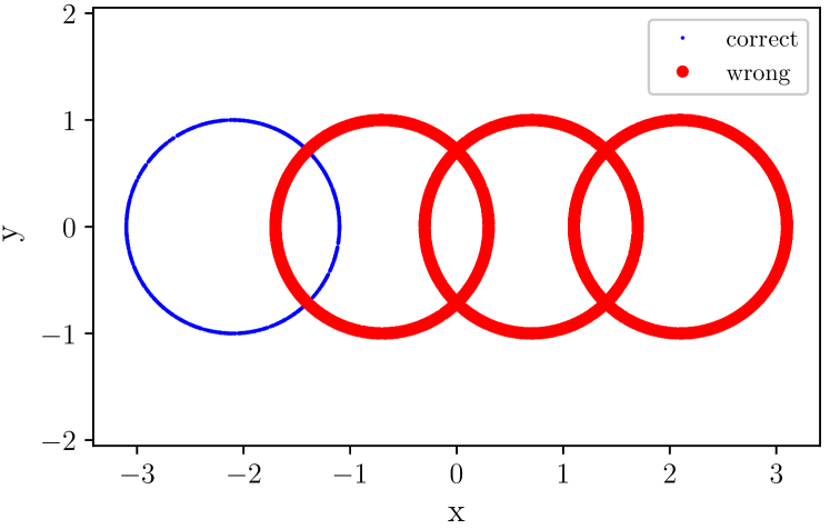
To further verify the effectiveness of the correction algorithm. We consider a more severe test with the corruption rate . That is, 90% of the data are corrupted. The corruption probability is taken as , which does not satisfy the condition (11). We show the history of the test accuracy during the training in Fig. 4 for the cases with and without the correction step. We see that in this severe test, the correction algorithm can still attain a test accuracy near , whereas the standard neural network without the correction step produce a test accuracy around . This is due to the fact that corruption is biased towards . Most of the samples have the label and hence the neural network tends to classify every feature into the second class. This is illustrated by the prediction plot in 5. With the correction algorithm applied, such bias is eliminated and the classification becomes almost completely recovered.


Example 2: Multiple-class Classification
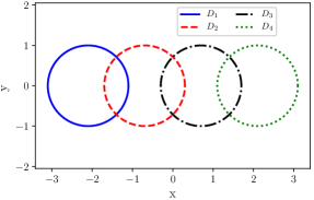
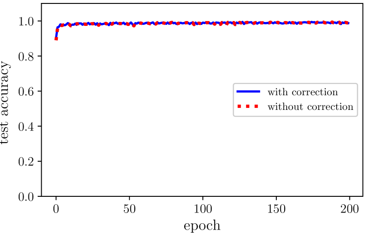
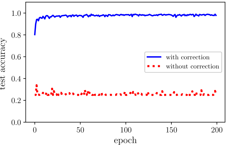
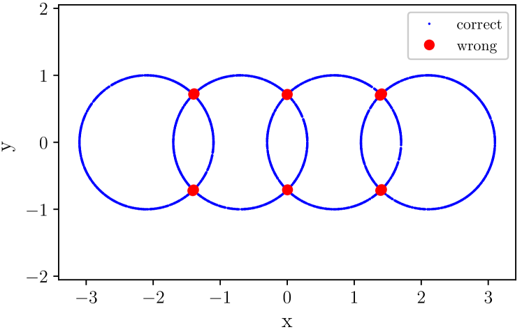
We further test our algorithm with multiple-class classification problems. In this example we consider the classification of classes, consisting of four unit circles with centers at , , and respectively, as shown in Fig. 6. The training samples are drawn from the uniform distribution over . We take samples with samples for each class. The labels are corrupted with a corruption distribution probability of . For the corruption ratio, we test two cases and . In the first case the condition (9) is satisfied and the classification can be completely recoverred without any correction, whereas in the second case, the condition (9) is violated and a correction step is necessary to recover the classification.
We use the same neural network architecture as in Example 1. Both of the CCE and SE loss functions are considered. The accuracy is tested on a set of clean data. In Fig. 7, the history of the test accuracy during the training is presented for both cases, with and without the correction step. It is observed that for the case , the classification is always completely recovered, regardless whether the correction step is added or not. For the case, where the condition 9 is not satisfied, the classifier without the correction produce a test accuracy around , whereas the correction step can recover the classification and attain an accuracy almost . This difference can be more clearly observed in Fig. 8, where the prediction results for the case are presented. Since the corruption distribution is biased towards the first class, the trained classifier (without correction) predicts the first class accurately but wrongly produces predictions for the other three classes. The correction procedure helps recover the classification, except for those not-well-defined samples that lie at the intersections of two neighboring classes


Example 3: MINST Dataset
Next, we test the applicability of the proposed correction algorithm on classification of the MINST hand-written digits data set [15], with corrupted labels. The labels are corrupted with a fixed corruption distribution . By the condition (9), the classification can be completely recovered if the corruption ratio .
The classifier is constructed by using a convolutional neural network (CNN), which consists of one 2D convolution layer of filters with size . It is followed by a max pooling layer and then the other 2D convolution layer of filters. At last a dense layer with nodes is added. To regularize the network, two dropout layers with dropout rate and are added, both before and after the dense layers. The activation functions are taken to be ReLU except in the output layer, where the softmax function is employed.
The trained model is tested on clean testing data, and we record the test accuracy for different corruption ratio in Table 1 for the CCE loss and in Table 2 for the SE loss. In both experiments, we record the test accuracy both with and without correction, as well as the number of epochs used in the training. We clearly observed the improvement in the test accuracy with the help of the correction step, especially when the the corruption ratio is greater than . When the corruption ratio is , the noise and corruption in the dataset is so overwhelming, combined with the limited number of training samples in MNIST, that no amount of correction can help to recover the classification.
| corruption ratio | test accuracy | corrected test accuracy | # epochs |
|---|---|---|---|
| 0% | 0.9922 | 0.9922 | 12 |
| 10% | 0.9873 | 0.9875 | 10 |
| 20% | 0.9842 | 0.9858 | 8 |
| 30% | 0.9781 | 0.9836 | 7 |
| 40% | 0.9412 | 0.9745 | 5 |
| 50% | 0.8655 | 0.9710 | 6 |
| 60% | 0.5051 | 0.9607 | 7 |
| 70% | 0.1294 | 0.9331 | 9 |
| 80% | 0.0981 | 0.7875 | 10 |
| 90% | 0.0980 | 0.0954 | 4 |
| corruption ratio | test accuracy | corrected test accuracy | # epochs |
|---|---|---|---|
| 0% | 0.9914 | 0.9914 | 11 |
| 10% | 0.9897 | 0.9898 | 7 |
| 20% | 0.9868 | 0.9886 | 8 |
| 30% | 0.9755 | 9.9799 | 5 |
| 40% | 0.9529 | 0.9765 | 10 |
| 50% | 0.9480 | 0.9712 | 4 |
| 60% | 0.5599 | 0.9590 | 7 |
| 70% | 0.1207 | 0.9330 | 9 |
| 80% | 0.0998 | 0.7692 | 13 |
| 90% | 0.0980 | 0.0958 | 4 |
Example 4: Fashion MNIST Dataset
Our last example is the fashion MNIST dataset [34], consisting of gray-scale images of fashion products from categories. The data set has samples in total. We take as training data and the other as testing data.
The labels of the training samples are corrupted according to a fixed corruption distribution with different corruption ratios. We use the same neural network structure as that for Example 3. In Table 3 and Table 4, we record the test accuracy for the model trained with the CCE and SE loss functions, both before and after applying the correction algorithm. Again, significant improvement in accuracy is observed, except the extreme case where the corruption ratio is .
| corruption ratio | test accuracy | corrected test accuracy | # epochs |
|---|---|---|---|
| 0 % | 0.9204 | 0.9204 | 10 |
| 10% | 0.9080 | 0.9080 | 7 |
| 20% | 0.9098 | 0.9106 | 9 |
| 30% | 0.8975 | 0.9013 | 10 |
| 40% | 0.8770 | 0.8928 | 8 |
| 50% | 0.7880 | 0.8798 | 11 |
| 60% | 0.5947 | 0.8771 | 7 |
| 70% | 0.1374 | 0.8421 | 9 |
| 80% | 0.1001 | 0.7397 | 13 |
| 90% | 0.1000 | 0.1000 | 4 |
| corruption ratio | test accuracy | corrected test accuracy | # epochs |
|---|---|---|---|
| 0% | 0.9193 | 0.9193 | 10 |
| 10% | 0.9148 | 0.9145 | 7 |
| 20% | 0.9057 | 0.9069 | 14 |
| 30% | 0.8937 | 0.8951 | 5 |
| 40% | 0.8806 | 0.8879 | 6 |
| 50% | 0.8276 | 0.8804 | 8 |
| 60% | 0.5792 | 0.8735 | 7 |
| 70% | 0.1166 | 0.8375 | 10 |
| 80% | 0.1000 | 0.7519 | 13 |
| 90% | 0.1000 | 0.1000 | 7 |
6 Conclusion
In this paper, we proposed a correction algorithm for the classification problems, where the data available are potentially corrupted. When the model is trained by minimizing the CCE or SE loss function, given sufficiently large amount of data, it is theoretically shown that the classification can be completely recovered by adding a correction step to the trained model. In particular, if the training data contains unlabeled samples, a random label assignment according to the uniform distribution would make the classification completely recovered. The proposed algorithm is non-intrusive and can be coupled with many models, such as support vector machines, neural networks of various architectures and so on. Numerical experiments were conducted with the proposed correction procedure applied to the neural networks models for two academic examples as well as two benchmark real-world tests with complicated and limited dataset. Numerical results confirmed the theoretical findings and demonstrated that, when the data labels contain corruptions, the proposed correction algorithm gives satisfactory test accuracy and can effectively eliminate the impact of label corruptions.
Appendix A Proof of Theorem 1
Proof.
Note that
where
For each , we consider the minimum of the function
subject to
where is the probability simplex.
For the CCE loss function, we have
Using the Lagrangian multiplier method, we consider the Lagrange function
At the minimal point, the gradient of the Lagrange function must be zero. This yields
| (64) |
Solving (64), one obtains
Hence, the function that minimizes satisfies:
for .
For the SE loss function, we have
Using the Lagrangian multiplier method, we consider the Lagrange function
At the minimal point, the gradient of the Lagrange function must be zero. This yields
which further implies
| (65) |
Solving (65), one obtains
Hence, the function that minimizes satisfies:
for .
The proof is complete. ∎
References
- [1] M. Abadi, A. Agarwal, P. Barham, E. Brevdo, Z. Chen, C. Citro, G. S. Corrado, A. Davis, J. Dean, M. Devin, S. Ghemawat, I. Goodfellow, A. Harp, G. Irving, M. Isard, Y. Jia, R. Jozefowicz, L. Kaiser, M. Kudlur, J. Levenberg, D. Mané, R. Monga, S. Moore, D. Murray, C. Olah, M. Schuster, J. Shlens, B. Steiner, I. Sutskever, K. Talwar, P. Tucker, V. Vanhoucke, V. Vasudevan, F. Viégas, O. Vinyals, P. Warden, M. Wattenberg, M. Wicke, Y. Yu, and X. Zheng, TensorFlow: Large-scale machine learning on heterogeneous systems, 2015, http://tensorflow.org/. Software available from tensorflow.org.
- [2] J. P. Brooks, Support vector machines with the ramp loss and the hard margin loss, Operations research, 59 (2011), pp. 467–479.
- [3] F. Chollet et al., Keras. https://keras.io, 2015.
- [4] B. Frénay and M. Verleysen, Classification in the presence of label noise: a survey, IEEE transactions on neural networks and learning systems, 25 (2014), pp. 845–869.
- [5] A. Ghosh, H. Kumar, and P. Sastry, Robust loss functions under label noise for deep neural networks, in Thirty-First AAAI Conference on Artificial Intelligence, 2017.
- [6] A. Ghosh, N. Manwani, and P. Sastry, Making risk minimization tolerant to label noise, Neurocomputing, 160 (2015), pp. 93–107.
- [7] A. Graves, A.-r. Mohamed, and G. Hinton, Speech recognition with deep recurrent neural networks, in Acoustics, speech and signal processing (icassp), 2013 ieee international conference on, IEEE, 2013, pp. 6645–6649.
- [8] E. Haber and L. Ruthotto, Stable architectures for deep neural networks, Inverse Problems, 34 (2017), p. 014004.
- [9] K. He, X. Zhang, S. Ren, and J. Sun, Deep residual learning for image recognition, in Proceedings of the IEEE conference on computer vision and pattern recognition, 2016, pp. 770–778.
- [10] D. Hendrycks, M. Mazeika, D. Wilson, and K. Gimpel, Using trusted data to train deep networks on labels corrupted by severe noise, in Advances in Neural Information Processing Systems, 2018, pp. 10477–10486.
- [11] L. Jiang, Z. Zhou, T. Leung, L.-J. Li, and L. Fei-Fei, Mentornet: Regularizing very deep neural networks on corrupted labels, arXiv preprint arXiv:1712.05055, 4 (2017).
- [12] A. Khetan, Z. C. Lipton, and A. Anandkumar, Learning from noisy singly-labeled data, arXiv preprint arXiv:1712.04577, (2017).
- [13] D. P. Kingma and J. Ba, Adam: A method for stochastic optimization, arXiv preprint arXiv:1412.6980, (2014).
- [14] J. Larsen, L. Nonboe, M. Hintz-Madsen, and L. K. Hansen, Design of robust neural network classifiers, in Proceedings of the 1998 IEEE International Conference on Acoustics, Speech and Signal Processing, ICASSP’98 (Cat. No. 98CH36181), vol. 2, IEEE, 1998, pp. 1205–1208.
- [15] Y. LeCun, B. E. Boser, J. S. Denker, D. Henderson, R. E. Howard, W. E. Hubbard, and L. D. Jackel, Handwritten digit recognition with a back-propagation network, in Advances in neural information processing systems, 1990, pp. 396–404.
- [16] B. Li, Y. Wang, A. Singh, and Y. Vorobeychik, Data poisoning attacks on factorization-based collaborative filtering, in Advances in neural information processing systems, 2016, pp. 1885–1893.
- [17] Y. Li, J. Yang, Y. Song, L. Cao, J. Luo, and L.-J. Li, Learning from noisy labels with distillation, in Proceedings of the IEEE International Conference on Computer Vision, 2017, pp. 1910–1918.
- [18] T. Liu and D. Tao, Classification with noisy labels by importance reweighting, IEEE Transactions on pattern analysis and machine intelligence, 38 (2016), pp. 447–461.
- [19] P. M. Long and R. A. Servedio, Random classification noise defeats all convex potential boosters, Machine learning, 78 (2010), pp. 287–304.
- [20] N. Manwani and P. Sastry, Noise tolerance under risk minimization, IEEE transactions on cybernetics, 43 (2013), pp. 1146–1151.
- [21] H. Masnadi-Shirazi and N. Vasconcelos, On the design of loss functions for classification: theory, robustness to outliers, and savageboost, in Advances in neural information processing systems, 2009, pp. 1049–1056.
- [22] A. Menon, B. Van Rooyen, C. S. Ong, and B. Williamson, Learning from corrupted binary labels via class-probability estimation, in International Conference on Machine Learning, 2015, pp. 125–134.
- [23] V. Mnih and G. E. Hinton, Learning to label aerial images from noisy data, in Proceedings of the 29th International conference on machine learning (ICML-12), 2012, pp. 567–574.
- [24] V. Nair and G. E. Hinton, Rectified linear units improve restricted boltzmann machines, in Proceedings of the 27th international conference on machine learning (ICML-10), 2010, pp. 807–814.
- [25] N. Natarajan, I. S. Dhillon, P. K. Ravikumar, and A. Tewari, Learning with noisy labels, in Advances in neural information processing systems, 2013, pp. 1196–1204.
- [26] D. F. Nettleton, A. Orriols-Puig, and A. Fornells, A study of the effect of different types of noise on the precision of supervised learning techniques, Artificial Intelligence Review, 33 (2010), pp. 275–306.
- [27] C. G. Northcutt, T. Wu, and I. L. Chuang, Learning with confident examples: Rank pruning for robust classification with noisy labels, arXiv preprint arXiv:1705.01936, (2017).
- [28] G. Patrini, A. Rozza, A. Krishna Menon, R. Nock, and L. Qu, Making deep neural networks robust to label noise: A loss correction approach, in Proceedings of the IEEE Conference on Computer Vision and Pattern Recognition, 2017, pp. 1944–1952.
- [29] M. Ren, W. Zeng, B. Yang, and R. Urtasun, Learning to reweight examples for robust deep learning, arXiv preprint arXiv:1803.09050, (2018).
- [30] J. Steinhardt, P. W. W. Koh, and P. S. Liang, Certified defenses for data poisoning attacks, in Advances in neural information processing systems, 2017, pp. 3517–3529.
- [31] S. Sukhbaatar, J. Bruna, M. Paluri, L. Bourdev, and R. Fergus, Training convolutional networks with noisy labels, arXiv preprint arXiv:1406.2080, (2014).
- [32] B. Van Rooyen, A. Menon, and R. C. Williamson, Learning with symmetric label noise: The importance of being unhinged, in Advances in Neural Information Processing Systems, 2015, pp. 10–18.
- [33] A. Veit, N. Alldrin, G. Chechik, I. Krasin, A. Gupta, and S. Belongie, Learning from noisy large-scale datasets with minimal supervision, in Proceedings of the IEEE Conference on Computer Vision and Pattern Recognition, 2017, pp. 839–847.
- [34] H. Xiao, K. Rasul, and R. Vollgraf, Fashion-mnist: a novel image dataset for benchmarking machine learning algorithms, arXiv preprint arXiv:1708.07747, (2017).
- [35] T. Xiao, T. Xia, Y. Yang, C. Huang, and X. Wang, Learning from massive noisy labeled data for image classification, in Proceedings of the IEEE conference on computer vision and pattern recognition, 2015, pp. 2691–2699.
- [36] J. Zhang and Y. Yang, Robustness of regularized linear classification methods in text categorization, in Proceedings of the 26th annual international ACM SIGIR conference on Research and development in informaion retrieval, ACM, 2003, pp. 190–197.
- [37] Z. Zhang and M. Sabuncu, Generalized cross entropy loss for training deep neural networks with noisy labels, in Advances in Neural Information Processing Systems, 2018, pp. 8792–8802.
- [38] X. Zhu and X. Wu, Class noise vs. attribute noise: A quantitative study, Artificial intelligence review, 22 (2004), pp. 177–210.