Information Freshness for Timely Detection of Status Changes

Abstract

In this paper, we aim to establish the connection between Age of Information (AoI) in network theory, information uncertainty in information theory, and detection delay in time series analysis. We consider a dynamic system whose state changes at discrete time points, and a state change won’t be detected until an update generated after the change point is delivered to the destination for the first time. We introduce an information theoretic metric to measure the information freshness at the destination, and name it as generalized Age of Information (GAoI). We show that under any state-independent online updating policy, if the underlying state of the system evolves according to a stationary Markov chain, the GAoI is proportional to the AoI. Besides, the accumulative GAoI and AoI are proportional to the expected accumulative detection delay of all changes points over a period of time. Thus, any (G)AoI-optimal state-independent updating policy equivalently minimizes the corresponding expected change point detection delay, which validates the fundamental role of (G)AoI in real-time status monitoring. Besides, we also investigate a Bayesian change point detection scenario where the underlying state evolution is not stationary. Although AoI is no longer related to detection delay explicitly, we show that the accumulative GAoI is still an affine function of the expected detection delay, which indicates the versatility of GAoI in capturing information freshness in dynamic systems.

I Introduction

Recently, how to quantify and optimize information freshness in sensing, communication and computing systems has attracted growing attention from different communities. Various metrics have been proposed to measure information freshness. Among them, perhaps the most prevalent one is Age of Information (AoI) [1]. Originally proposed for a single-node monitoring system that keeps sending time-stamped status updates to a destination, the metric quantifies the freshness of information from the destination’s perspective. Specifically, at time $t$, the AoI at the destination is defined as $t-\delta(t)$, where $\delta(t)$ is the generation time (time stamp) of the freshest received update at the destination. With this definition, the AoI performance has been characterized for various updating policies in different systems  [2, 3, 4, 5]. AoI optimization from the perspectives of sampling, transmission scheduling and coding has also been investigated under various system constraints  [6, 7, 8, 9, 10, 11, 12, 13, 14, 15, 16, 17, 18, 19, 20, 21].

Even though AoI can be used as a measure of “staleness” of the status information in a system, it does not take the dynamics of the underlying status evolution into consideration. Recently, there are a few attempts to take the properties of the monitored signal into the definition of information freshness. A metric called “Age of Synchronization” (AoS) is proposed in [22]. It refers to the duration since the destination became desynchronized with the source. In the same spirit, another metric called “Age of Incorrect Information” (AoII) is proposed in [23]. AoII takes both the time that the monitor is unaware of the correct status of the system and the difference between the current estimate at the monitor and the actual state of system into the definition. With particular penalty functions, AoII reduces to AoS. Reference [24] proposes to use the mutual information between the real-time source value and the delivered samples at the receiver to quantify the freshness of the information contained in the delivered samples. It shows that for a time-homogeneous Markov chain, the mutual information can be expressed as a non-negative and non-increasing function of the age. In [25], a metric called “Value of Information” (VoI) is introduced to facilitate packet scheduling for low-error Kalman filter based estimation. VoI depends on the age of the packet, as well as the mutual information between the packet content and the system status, which is equivalent to the variance of the noise associated with the measurement. Generally speaking, how to define a universal information freshness metric that accounts for dynamically evolving system states remains open.

In this paper, we propose an information theoretic measure of information freshness by taking the dynamics of the monitored system into account, where we introduce a two-dimensional discrete-time Markov chain to model the underlying state changes. Our main contributions are three-fold:

First, the introduced information theoretic measure generalizes the definition of AoI. It takes the age of updates and the dynamics of the monitored system into the definition, and suggests a unified approach to define proper age penalty functions [26] for various dynamic systems.

Second, we establish fundamental relationship between AoI and the expected detection delay of status changes under any state-independent online updating policies. Such relationship validates the critical role of AoI in real-time status monitoring when the system evolution is stationary. It enables us to safely decouple the properties of the underlying system from the design of age-optimal sampling, scheduling and coding policies, without compromising the effectiveness of the delivered updates on tracking status changes of the system.

Third, we show that the generalized AoI is an affine function of the expected detection delay in an adapted Bayesian change point detection setting. This observation suggests that GAoI is a proper measure of information freshness even when the underlying system evolution is not stationary.

II System Model

Consider a single-node status monitoring scenario where a sensor monitors the status of an underlying system and sends updates to a destination through a communication channel. In order to capture the dynamics of the monitored system, we consider a discrete-time model, where the status of the system in each time slot $n$ is denoted as $X_{n}$. We assume $X_{n}$ takes values from a finite alphabet $\mathcal{X}$. At the beginning of time slot $n$, $X_{n}$ may stay the same as $X_{n-1}$, or change to a different value. We let $T_{n}\in\{0,1,2,\ldots\}$ denote the number of time slots the system has stayed in the current status. Then,

$$T_{n}=\left\{\begin{array}[]{ll}T_{n-1}+1,&\mbox{ if }X_{n}=X_{n-1},\\ 0,&\mbox{ if }X_{n}\neq X_{n-1}.\end{array}\right.$$

We assume the evolution of $\{T_{n}\}$ depends on the current status $X_{n}$ in general. Specifically, we denote $q_{i}(x):=\mathbb{P}[T_{n+1}=0|T_{n}=i,X_{n}=x]$, and denote the corresponding transition matrix as $P_{T}(x)$. Besides, if $T_{n}=0$, i.e., a status change happens at the beginning of time slot $n$, $X_{n}$ evolves according to a Markov chain with transition matrix $P_{X}$, as illustrated in Fig. 1. Denote the status of the system at time $n$ as $U_{n}:=(X_{n},T_{n})$. We can show that $U_{n}$ evolves according to a two-dimensional Markov chain. Essentially, such a model accommodates the scenario where $\{X_{n}\}$ is Markovian, as well as certain scenarios where $\{X_{n}\}$ cannot be simply modeled as a Markov chain, thus is more general in modeling dynamic status changes.

Assume each state update sampled at time $n$ is a time-stamped tuple $U_{n}:=(X_{n},T_{n})$, i.e., it does not just contain the time-stamped status $X_{n}$, but also the duration that the system has stayed in the current status. The receiver tracks the system status based on received updates. The objective of this work is to investigate the fundamental impact of information freshness on the timely detection of status changes. As a first step, we focus on state-independent online policies defined as follows.

Definition 1 (State-independent online updating policies)

Let $s_{1},s_{2},\ldots\in{\mathbb{N}}$ be the sampling time points and $d_{1},d_{2},\ldots\in{\mathbb{N}}$ be the corresponding delivery times of the updates $U_{s_{1}}$, $U_{s_{2}}$, $\ldots$ under an updating policy, where we let $d_{i}=\infty$ if the $i$th update is never delivered. If $s_{i}$ only depends on previous sampling points $\{s_{j}\}_{j=1}^{i-1}$ and up-to-date delivery times $\{d_{j}:d_{j}\leq s_{i}\}$, and $d_{i}$s are independent with $\{U_{n}\}$, the policy is called a state-independent online updating policy.

We also formally define detection delay as follows.

Definition 2 (Detection delay of status changes)

If the system status changes at the beginning of time slot $n$, i.e., $T_{n}=0$, the detection delay of this status change equals $\min\{d_{i}:s_{i}\geq T_{n}\}-T_{n}$.

The definition of detection delay is intuitive in the sense that a status change won’t be detected until a status update collected after the change is delivered to the destination for the first time. From an information theoretic perspective, if multiple status changes happen between the sampling points of two consecutively delivered updates, as shown in Fig. 2, the destination won’t be able to locate all of them except the last one based on $U_{\delta(n)}$ only. However, we still consider them to be detected in order to properly measure the detection delay performance of the updating schemes.

Figure 1: An example of the discrete-time state transition model where $\mathcal{X}=\{1,2,3\}$.

III Information Theoretic Characterization of Information Freshness

Assume the latest status update at the destination at time $n$ was sampled at time $\delta(n)$. Then, the instantaneous AoI at the destination is $n-\delta(n)$. We propose the following metric as an information staleness measure at the destination at time $n$:

$$\Phi(n):=H(U^{\delta(n)+1:n}|U_{\delta(n)}),$$ (1)

where $U^{n:n+k}:=\{U_{n},U_{n+1},\ldots,U_{n+k}\}$. Intuitively, $\Phi(n)$ captures the “novelty” in random process $\{U_{n}\}$ since time $\delta(n)$, which also indicates the uncertainty level at the destination regarding the monitored system status over duration $[\delta(n)+1,n]$. We term it as generalized Age of Information (GAoI) in this paper.

The GAoI defined in (1) essentially measures information freshness from an ensemble’s perspective, i.e., it averages over all possible realizations of $\{U_{n}\}$. Therefore it is state-independent, i.e., it is independent with the information content of the received updates (i.e., $U_{\delta(n)}$); Rather, it only relies on stochastic information of the state evolution process (i.e., $\{P_{T}(x)\}$ and $P_{X}$), as well as the time stamps of received updates.

Intuitively, the information contained in $U_{\delta(n)}$ may indicate how fast the system status may change from the previous status, and how much uncertainty/novelty is generated since the latest update was generated. This motivates the definition of state-dependent GAoI as follows.

Define

$$\Phi(n|U_{\delta(n)}=u)=H(U^{\delta(n)+1:n}|U_{\delta(n)}={u}),$$ (2)

i.e., the uncertainty in system states over $[\delta(n)+1,n]$ given the latest observation $U_{\delta(n)}=u$.

Then, based on the definition of conditional entropy, we have

$$\Phi(n)=\sum_{u}\Phi(n|U_{\delta(n)}=u)\cdot\mathbb{P}[U_{\delta(n)}=u].$$ (3)

The discrete-time status evolution model enables us to explicitly discuss the relationship between GAoI, AoI and the detection delay of status changes. In the following, we investigate two scenarios, and establish their relationships.

Figure 2: AoI evolution with given status change points. $\times$ represents status changes, $\Circle$ represents sampling points, and solid circle represents delivery time of an update. $\Gamma_{i}$ is the detection delay for the $i$th status change.

IV Stationary Markovian State Evolution

In this section, we focus on stationary Markovian state evolution models.

Proposition 1

Assume $(X_{n},T_{n})$ evolves according to a stationary Markov chain $\mathcal{C}$ defined by transition matrices $P_{X}$ and $\{P_{T}(x)\}_{x\in\mathcal{X}}$. Then,

$$\Phi(n) =(n-\delta(n))\cdot H(P_{X},\{P_{T}(x)\}_{x\in\mathcal{X}}),$$

where $H(P_{X},\{P_{T}(x)\}_{x\in\mathcal{X}})$ is the entropy rate of $\mathcal{C}$.

Due to space limitation, we omit the proofs of propositions and corollaries in this paper. Proposition 1 can be proved based on the property of stationary Markov chains. It indicates that the information freshness measure $\Phi(n)$ is proportional to the instantaneous age $n-\delta(n)$ if $H(P_{X},\{P_{T}(x)\}_{x\in\mathcal{X}})\neq 0$, which validates the effectiveness of AoI in capturing uncertainty in the system status from the destination’s perspective.

Besides, compared with AoI which only depends on time, $\Phi(n)$ also captures the dynamics of the underlying status evolution. For systems with frequent state changes, or with very dynamic state transitions, $\Phi(n)$ grows quickly as age increases, which implies that the information gets stale quickly. On the other hand, in systems with more deterministic state changes, information will “age” at a slower rate.

One extreme case is when the status of the system evolves in a periodic pattern, i.e., given an initial status $X_{0}$, the system evolves according to a cycle over the states in $\mathcal{X}$. Thus, $\Phi(n)=0$, i.e., $U_{\delta(n)}$ will never get expired, since it can be used to accurately predict the state of the system in any upcoming time. Therefore, AoI itself cannot be used for a measure of information freshness for this scenario. This special case illustrates the importance of taking the dynamics of status evolution into the definition of information freshness.

Proposition 2

Assume the stationary distribution of $(X_{n},T_{n})$ exists, and denote it as $\{\mu_{x,i}\}_{x\in\mathcal{X},i\in\mathbb{Z}_{+}}$, where $\mu_{x,i}=\mathbb{P}[(X_{n},T_{n})=(x,i)]$. Then, $H(P_{X},\{P_{T}(x)\}_{x\in\mathcal{X}})$ equals

$$\sum_{x\in\mathcal{X}}\mu_{x,0}\sum_{i=0}^{\infty}\prod_{j=0}^{i-1}(1-q_{j}(x))[H(q_{i}(x),1-q_{i}(x))+q_{i}(x)H(\mathbf{p}_{x})],$$

where $\mathbf{p}_{x}$ is the row associated with status $x$ in $P_{X}$, and $H(\pi)$ is the entropy of distribution $\pi$.

Corollary 1

If $P_{T}(x)$ is homogeneous, i.e., $P_{T}(x)=P_{T}$ for all state $x\in\mathcal{X}$, then, the entropy rate of the Markov chain $\mathcal{C}$ equals

$$H(P_{X},P_{T})=H(P_{T})+H(P_{X})\mathbb{P}(T_{n}=0).$$ (4)

Our main result is summarized as follows.

Theorem 1

Assume the monitor is informed of the initial system state at time 0. Then, under any state-independent online updating policy,

$$\frac{\bar{\Phi}(T)}{H(P_{X},\{P_{T}(x)\})}=\bar{\Delta}(T)=\frac{\bar{\Gamma}(T)}{\mathbb{P}(T_{n}=0)},$$

where $\bar{\Phi}(T):=\sum_{n=1}^{T}\Phi(n)$, $\bar{\Gamma}(T)$ is the expected total detection delay of the state changes over $[1,T]$, and $\bar{\Delta}(T)$ is the expected total AoI experienced at the destination over $[1,T]$.

Proof:  Consider the sampling times and update delivery times under a state-independent online updating policy. For ease of exposition, let $s_{i}$ and $d_{i}$ be the $i$th sampling time and the corresponding delivery time. Consider the first $T$ time slots $[1,T]$ during which $K$ updates are delivered. We collectively denote the delivery times as $\{d_{i}\}_{i=1}^{K}$ and the corresponding sampling times as $\{s_{i}\}_{i=1}^{K}$. We also define $d_{0}=s_{0}=0$ and $d_{K+1}=s_{K+1}=T$. Without loss of generality, we can assume $d_{i}<d_{j}$ whenever $s_{i}<s_{j}$. In fact, if there exists $s_{j}\geq s_{i}$ such that $d_{j}\leq d_{i}$, the information delivered at time $d_{i}$ is stale compared to the previously received information $U_{s_{j}}$. Thus, we can exclude such updates without affecting the (G)AoI evolution or detection delay. Define the detection delay of a status change at time $n$ $(n\leq T)$ restricted to $[1,T]$ as $\Gamma=\min\{d_{i}:s_{i}\geq n,i\leq K+1\}-n$. The expected total detection delay over $[1,T]$ can be expressed as

$$\bar{\Gamma}(T) =\mathbb{P}(T_{n}=0)\sum_{i=0}^{K}\sum_{j=s_{i}+1}^{s_{i+1}}(d_{i+1}-j),$$ (5)

where the equality is based on the fact that $\mathbb{P}(T_{n}=0)$ is a constant for all $n$ under the assumption that $\{U_{n}\}$ is a stationary Markov chain. Then, the expected total detection delay over $[1,T]$ scaled by $1/\mathbb{P}(T_{n}=0)$ is

$$\frac{\bar{\Gamma}(T)}{\mathbb{P}(T_{n}=0)} =\frac{1}{2}T^{2}-\frac{1}{2}T-\sum_{i=1}^{K}s_{i}(d_{i+1}-d_{i}).$$ (6)

The expected AoI experienced over $[1,T]$ is

$$\bar{\Delta}(T) ={\sum_{j=0}^{K+1}\sum_{i=0}^{d_{j+1}-d_{j}-1}(d_{j}-s_{j}+i)}$$ (7)

$$=\frac{1}{2}T^{2}-\frac{1}{2}T-\sum_{i=1}^{K}s_{i}(d_{i+1}-d_{i}).$$ (8)

Hence, $\bar{\Gamma}(T)=\bar{\Delta}(T)\cdot\mathbb{P}(T_{n}=0)$. We note that this equation holds for any possible realizations of $s_{i}$s and $d_{i}$s under a state-independent online updating policy. Thus, it still holds if we take expectations with respect to $s_{i}$s and $d_{i}$s. The first equality then follows from Proposition 1.  $\blacksquare$

Theorem 1 validates the fundamental role of information freshness on timely detection of status changes. It indicates that minimizing AoI through state-independent sampling, transmission scheduling or coding is equivalent to minimizing the expected detection delay of the status changes in the system.

V Non-stationary Markovian State Evolution

The result in Section IV relies on the stationary Markovian state evolution assumption. It is also intuitive that under the stationary Markovian assumption, $\Phi(n)$ scale proportionally to the instantaneous age at the destination. However, such assumptions are quite restrictive in practice. This motivates us to investigate a broader class of status change models where the stationary assumption may not hold. While this seems challenging for a general setting, as a first step, we consider the following status change model, which is adapted from the classical Bayesian change point detection model in the literature.

We assume the system status starts with an initial state $0$ at $n=0$. At an unknown change point $\theta\in{\mathbb{N}}$, the system status changes to $1$. Under the Bayesian setting, it assumes that $\theta$ is a random variable following a geometric distribution, i.e., $\mathbb{P}[\theta=\tau]=p(1-p)^{\tau-1}$, $\tau=1,2,\ldots$.

We can show that the system status $\{X_{n}\}$ can be modeled as a Markov chain shown in Fig. 3. Since it has an absorbing state 1, and the initial state $X_{0}=0$, the Markov chain is no longer stationary.

Since the state evolution can be characterized by a one-dimensional Markov chain $\{X_{n}\}$, the information theoretic definitions of information freshness in Eqns. (1) and (2) are equivalent to the following definitions, respectively:

$$\Phi(n)=H(X^{\delta(n)+1:n}|X_{\delta(n)}),$$ (9)

$$\Phi(n|X_{\delta(n)}=x)=H(X^{\delta(n)+1:n}|X_{\delta(n)}=x).$$ (10)

Figure 3: Equivalent Markov chain for the Bayesian change point model.

We have the following observations.

Proposition 3

Under the Bayesian change point model,

$$\Phi(n|X_{\delta(n)}=0) =0,$$

$$\Phi(n|X_{\delta(n)}=1) =H(p,\cdots,(1-p)^{n-\delta(n)-1}p,(1-p)^{n-\delta(n)}),$$

where $H(p_{1},p_{2},\cdots,p_{n})=-\sum_{i}p_{i}\log{p_{i}}$.

Theorem 2

Under any state-independent online updating policy,

$$\bar{\Phi}(T)=\frac{H(p,1-p)}{p}\bar{\Gamma}(T)+C(T),$$

where $\bar{\Phi}(T):=\sum_{n=1}^{T}\Phi(n)$, $\bar{\Gamma}(T)$ is the expected detection delay of the state change over $[1,T]$, and $C(T)$ is a constant for fixed $T$.

Proof:  Denote $h(x)$ as

$$h(x):=H(p,\cdots,(1-p)^{x-1}p,(1-p)^{x}),\forall x\in{\mathbb{N}}.$$ (11)

Based on the definition of entropy, we have the following recursive formula:

$$h(x+1)=h(x)+(1-p)^{x}h(p).$$ (12)

Denote $h(1):=H(p,1-p)$. Then,

$$h(x)=\frac{1-(1-p)^{x}}{p}h(1).$$ (13)

Plugging (13) into the expression in Proposition 3, we have

$$\Phi(n|X_{\delta(n)}=0)=\frac{1-(1-p)^{n-\delta(n)}}{p}h(1).$$ (14)

Then, a uniform expression for the state-dependent GAoI is as follows:

$$\Phi(n|X_{\delta(n)}=x)$$

$$=\frac{1-(1-p)^{n-\delta(n)}}{p}h(1)\mathbf{1}_{X_{\delta(n)}=0},\quad x\in\{0,1\}.$$ (15)

Similar to the proof of Theorem 1, we consider the sampling points $s_{1},s_{2},\ldots,s_{K}$ and corresponding delivery points $d_{1},d_{2},\ldots,d_{K}$ of the $K$ updates delivered over $[1,T]$ under a given state-independent updating policy, as shown in Fig. 4. Without loss of generality, we assume $0<s_{1}<s_{2}<\ldots<s_{K}<T$ and $0<d_{1}<d_{2}<\ldots<d_{K}<T$. We define $s_{0}=d_{0}=0$ and $s_{K+1}=d_{K+1}=T$ for ease of exposition.

The accumulative generalized GAoI can be expressed as

$$\sum_{n=1}^{T}\Phi(n|X_{\delta(n)}=x)=\sum_{i=0}^{K}\sum_{j=d_{i}+1}^{d_{i+1}}\frac{1-(1-p)^{j-s_{i}}}{p}h(1)\mathbf{1}_{X_{s_{i}}=0}.$$

Taking expectation with respect to $x$, we have

$$\bar{\Phi}(T)$$

$$=\sum_{i=0}^{K}\sum_{j=d_{i}+1}^{d_{i+1}}\frac{1-(1-p)^{j-s_{i}}}{p}h(1)(1-p)^{s_{i}}$$

$$=\frac{h(1)}{p}\left(\frac{(1-p)[(1-p)^{T}-1]}{p}+\sum_{i=0}^{K}(d_{i+1}-d_{i})(1-p)^{s_{i}}\right).$$ (16)

On the other hand, the expected detection delay can be calculated as follows:

$$\bar{\Gamma}(T)$$

$$=\sum_{i=0}^{K}\sum_{j=s_{i}+1}^{s_{i+1}}(1-p)^{j-1}p(d_{i+1}-j)$$ (17)

$$=-\sum_{k=1}^{T}k(1-p)^{k-1}p+\sum_{i=0}^{K}\sum_{j=s_{i}+1}^{s_{i+1}}(1-p)^{j-1}pd_{i+1}$$ (18)

$$=-\sum_{k=1}^{T}k(1-p)^{k-1}p+\sum_{i=0}^{K}d_{i+1}[(1-p)^{s_{i}}-(1-p)^{s_{i+1}}]$$

$$=-T(1-p)^{T}-\sum_{k=1}^{T}k(1-p)^{k-1}p+\sum_{i=0}^{K}(d_{i+1}-d_{i})(1-p)^{s_{i}}.$$ (19)

Since the updating policy is state-independent, taking expectation of (16) and (19) with respect to $s_{i}$s, we have the proof complete.  $\blacksquare$

Figure 4: Generalized AoI evolution with given sampling times $s_{i}$s and delivery times $d_{i}$. $\times$ represents the change point, and $\Gamma$ represents the detection delay.

Theorem 2 indicates that GAoI is an affine function of the expected detection delay for the Bayesian change point model under any state-independent updating policy. We can verify that such relationship no longer holds between the AoI and the expected detection delay. Such result suggests that GAoI is a more accommodating measure of information freshness compared with AoI.

VI Simulation Results

Figure 5: Generalized AoI evolution with given sampling points.

In this section, we evaluate our results through simulations. We evaluate the AoI, GAoI and the status change detection delay under two state evolution models: a stationary two-state symmetric Markov chain and a Bayesian change point model.

VI-A Stationary Two-state Symmetric Markov chain

First, we consider a two-state symmetric Markov chain where the probability of status change is $p$, as illustrated in Fig. 5. We adopt two different updating schemes: The first one is uniform sampling with instant delivery where the sampling occurs at $n=50,100,\ldots$. The other one is greedy sampling policy with random delivery time, where the sampling happens whenever an update is delivered to the destination. We assume the delivery time of each update is uniformly distributed in $[20,80]$. We note that the sampling rates of the two schemes are actually the same, and both policies are state-independent. In this simulation, we fix $p=0.6$. For each updating policy, we generate $100$ sample paths, where the initial state is randomly selected according to the stationary distribution. For each sample path, we track the status changes and obtain the total detection delay, which is then averaged over $T$. We also track the AoI evolution and calculate its time average. As shown in Fig. 6, after scaling AoI by a factor of $\mathbb{P}(T_{n}=0)$, the ensemble average matches the ensemble average of the detection delay under both updating policies. This is consistent with the theoretical results in Theorem 1.

VI-B Bayesian Change Point Model

Next, we evaluate the relationship between the GAoI and the detection delay under a Bayesian change point model. We set $p=0.04$ and track the detection delay and the evolution of the state-dependent GAoI for each sample path under the two updating policies described in Sec. VI-A. We fix the sampling rate for the uniform sampling as once every five time slots. For the other policy, we let the random delivery time be uniformly distributed in $[2,8]$. We generate $2000$ sample paths over duration $[1,100]$. The ensemble average of the cumulative GAoI and the ensemble average of the detection delay are compared and plotted in Fig. 7. The GAoI curves are scaled by a factor of $\frac{p}{H(p,1-p)}$, as suggested in Theorem 2. It is noteworthy that the difference between the scaled GAoI and the detection delay is a constant under both updating policies, which corroborates the theoretical result in Theorem 2.

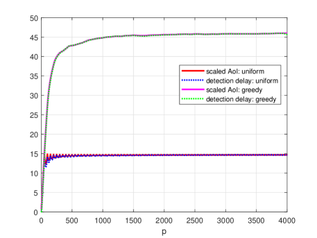
Figure 6: AoI and detection delay for a stationary Makovian status evolution model.

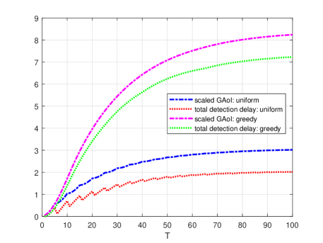
Figure 7: GAoI and detection delay for a Bayesian change point model.

VII Conclusions

In this paper, we introduce an information theoretic measure of information freshness and investigate its relationship between AoI and detection delay of status changes in a status monitoring system. Our results validates the fundamental role of AoI in timely change detection when the underlying system states evolve according to a stationary Markov chain. It also indicates that for a special non-stationary status change model, GAoI is a more proper measure. In the future, we will investigate the relationships between those metrics under state-dependent updating policies.

References

- [1] S. K. Kaul, R. D. Yates, and M. Gruteser, “Real-time status: How often should one update?” in IEEE INFOCOM, Orlando, FL, USA, Mar. 2012, pp. 2731–2735.
- [2] R. D. Yates and S. K. Kaul, “The age of information: Real-time status updating by multiple sources,” IEEE Transactions on Information Theory, vol. 65, no. 3, pp. 1807–1827, March 2019.
- [3] N. Pappas, J. Gunnarsson, L. Kratz, M. Kountouris, and V. Angelakis, “Age of information of multiple sources with queue management,” in IEEE International Conference on Communications (ICC), Jun. 2015, pp. 5935–5940.
- [4] E. Najm and R. Nasser, “Age of information: The gamma awakening,” in IEEE International Symposium on Information Theory (ISIT), Barcelona, Spain, Jul. 2016, pp. 2574–2578.
- [5] C. Kam, S. Kompella, G. D. Nguyen, and A. Ephremides, “Effect of message transmission path diversity on status age,” IEEE Trans. Inf. Theory, vol. 62, no. 3, pp. 1360–1374, Mar. 2016.
- [6] Y. Sun, Y. Polyanskiy, and E. Uysal-Biyikoglu, “Remote estimation of the Wiener process over a channel with random delay,” in IEEE International Symposium on Information Theory (ISIT), Jun. 2017, pp. 321–325.
- [7] Z. Jiang, S. Zhou, Z. Niu, and C. Yu, “A unified sampling and scheduling approach for status update in multiaccess wireless networks,” in IEEE INFOCOM, April 2019, pp. 208–216.
- [8] A. M. Bedewy, Y. Sun, and N. B. Shroff, “Optimizing data freshness, throughput, and delay in multi-server information-update systems,” in IEEE International Symposium on Information Theory (ISIT), Barcelona, Spain, Jul. 2016, pp. 2569–2573.
- [9] Y. Sun, E. Uysal-Biyikoglu, R. D. Yates, C. E. Koksal, and N. B. Shroff, “Update or wait: How to keep your data fresh,” in IEEE INFOCOM, San Francisco, CA, USA, Apr. 2016, pp. 1–9.
- [10] Q. He, D. Yuan, and A. Ephremides, “Optimal link scheduling for age minimization in wireless systems,” IEEE Transactions on Information Theory, vol. 64, no. 7, pp. 5381–5394, July 2018.
- [11] I. Kadota, A. Sinha, and E. Modiano, “Optimizing age of information in wireless networks with throughput constraints,” in IEEE INFOCOM, Apr. 2018.
- [12] B. Wang, S. Feng, and J. Yang, “When to preempt? age of information minimization under link capacity constraint,” Journal on Communications and Networking, vol. 21, no. 3, pp. 220–232, Jun. 2019.
- [13] B. Zhou and W. Saad, “Minimum age of information in the internet of things with non-uniform status packet sizes,” IEEE Transactions on Wireless Communications, pp. 1–1, 2019.
- [14] X. Wu, J. Yang, and J. Wu, “Optimal status update for age of information minimization with an energy harvesting source,” IEEE Transactions on Green Communications and Networking, vol. 2, no. 1, pp. 193–204, March 2018.
- [15] A. Arafa, J. Yang, S. Ulukus, and H. V. Poor, “Age-Minimal Transmission for Energy Harvesting Sensors with Finite Batteries: Online Policies,” IEEE Trans. on Information Theory, vol. 66, no. 1, pp. 534–556, Jan. 2020.
- [16] S. Feng and J. Yang, “Age of information minimization for an energy harvesting source with updating erasures: With and without feedback,” CoRR, vol. abs/1808.05141, 2018.
- [17] R. D. Yates, E. Najm, E. Soljanin, and J. Zhong, “Timely updates over an erasure channel,” in 2017 IEEE International Symposium on Information Theory (ISIT), Jun. 2017, pp. 316–320.
- [18] P. Mayekar, P. Parag, and H. Tyagi, “Optimal lossless source codes for timely updates,” IEEE International Symposium on Information Theory (ISIT), pp. 1246–1250, 2018.
- [19] J. Zhong, R. D. Yates, and E. Soljanin, “Timely Lossless Source Coding for Randomly Arriving Symbols,” ArXiv e-prints, Oct. 2018.
- [20] S. Feng and J. Yang, “Adaptive coding for information freshness in a two-user broadcast erasure channel,” in IEEE Global Communications Conference (Globecom), Hawaii, USA, Dec. 2019.
- [21] A. Baknina and S. Ulukus, “Coded status updates in an energy harvesting erasure channel,” in Conference on Information Sciences and Systems (CISS), Mar. 2018.
- [22] J. Zhong, R. D. Yates, and E. Soljanin, “Two freshness metrics for local cache refresh,” in IEEE International Symposium on Information Theory (ISIT), June 2018, pp. 1924–1928.
- [23] A. Maatouk, S. Kriouile, M. Assaad, and A. Ephremides, “The age of incorrect information: A new performance metric for status updates,” arXiv preprint arXiv:1907.06604, 2019.
- [24] Y. Sun and B. Cyr, “Information aging through queues: A mutual information perspective,” in 2018 IEEE 19th International Workshop on Signal Processing Advances in Wireless Communications (SPAWC), June 2018, pp. 1–5.
- [25] R. Singh, G. K. Kamath, and P. R. Kumar, “Optimal information updating based on value of information,” 2019.
- [26] A. Kosta, N. Pappas, A. Ephremides, and V. Angelakis, “Age and value of information: Non-linear age case,” in IEEE International Symposium on Information Theory (ISIT), Aachen, Germany, Jun. 2017, pp. 326–330.