hybrid-Lenstool: A self-consistent algorithm to model galaxy clusters with strong- and weak-lensing simultaneously

Abstract

We present a new galaxy cluster lens modeling approach, hybrid-Lenstool, that is implemented in the publicly available modeling software Lenstool. hybrid-Lenstool combines a parametric approach to model the core of the cluster, and a non-parametric (free-form) approach to model the outskirts. hybrid-Lenstool optimizes both strong- and weak-lensing constraints simultaneously (Joint-Fit), providing a self-consistent reconstruction of the cluster mass distribution on all scales. In order to demonstrate the capabilities of the new algorithm, we tested it on a simulated cluster. hybrid-Lenstool yields more accurate reconstructed mass distributions than the former Sequential-Fit approach where the parametric and the non-parametric models are optimized successively. Indeed, we show with the simulated cluster that the mass density profile reconstructed with a Sequential-Fit deviates form the input by $2-3\sigma$ at all scales while the Joint-Fit gives a profile that is within $1-1.5\sigma$ of the true value. This gain in accuracy is consequential for recovering mass distributions exploiting cluster lensing and therefore for all applications of clusters as cosmological probes. Finally we found that the Joint-Fit approach yields shallower slope of the inner density profile than the Sequential-Fit approach, thus revealing possible biases in previous lensing studies.

1 Introduction

Gravitational lensing is the bending of the light emitted by a background source as it grazes past the gravitational potential of a foreground object called the lens (for reviews see Kneib & Natarajan, 2011; Hoekstra et al., 2013; Bartelmann & Maturi, 2017). The lens can be any type of objects with masses ranging from a planet to a massive galaxy cluster. Here, we focus on the lensing of a background galaxy population by a massive, foreground cluster of galaxies. Gravitational lensing is observed in two regimes defined by the intensity of the distortions created by the gravitational potential of the lens: the strong-lensing regime where background galaxies are highly distorted into gravitational arcs and multiple images; and the weak-lensing regime wherein the distortions of background galaxies are small and need to be treated statistically.

While gravitational lensing generated by a galaxy lens was first observed in 1979 by Walsh, Carswell & Weymann (1979) with the multiply-imaged quasar Q0957 + 561A-B, astronomers had to wait until the late 1980’s to confirm the first observation of a gravitational arc in a galaxy cluster (Lynds & Petrosian, 1986; Soucail et al., 1987, 1988). Since then, gravitational lensing by galaxy clusters has emerged as a powerful tool to study the Universe. Indeed, gravitational lensing is a unique tool to map the mass distribution of the lenses as it is independent of their dynamical state, thereby providing crucial in-situ information on the physics of these objects. In the case of cluster lenses, a lot of work has been done from gravitational lensing mass maps and multi-wavelength analyses to constrain cluster physics (e.g., Kneib et al., 2003; Natarajan, Kneib & Smail, 2002; Clowe, Gonzalez & Markevitch, 2004; Bradač et al., 2006; Merten et al., 2011; Diego et al., 2015; Eckert et al., 2015; Jauzac et al., 2012, 2015; Mahler et al., 2018; Sharon et al., 2015, 2019), and dark matter properties (e.g., Natarajan et al., 2002, 2017; Bradač et al., 2008; Harvey et al., 2015; Harvey, Kneib & Jauzac, 2016; Harvey et al., 2017, 2019; Massey et al., 2015, 2018; Jauzac et al., 2016a, 2018). Moreover, lensing can give us hints on galaxy evolution (e.g. Natarajan et al., 1998; Limousin et al., 2007; Natarajan et al., 2009; Leauthaud et al., 2012, 2015; Li et al., 2016; Sifón et al., 2015; Niemiec et al., 2017), and on the distant Universe as lenses behave as cosmic telescopes and thus allow us to observe high-redshift galaxies (e.g. Atek et al., 2015, 2018; Alavi et al., 2016; Bouwens et al., 2017; D’Aloisio, Natarajan & Shapiro, 2014; Ishigaki et al., 2018; Kawamata et al., 2018), study highly magnified galaxies at intermediate redshifts (e.g. Teplitz et al., 2000; Bayliss et al., 2014; Johnson et al., 2017; Rigby et al., 2018; Rivera-Thorsen et al., 2019; Bayliss et al., 2019; Chisholm et al., 2019; Sharon et al., 2019), and/or lensed transients (e.g., Goobar et al., 2017; Kelly et al., 2015, 2018; Treu et al., 2016; Jauzac et al., 2016b; Diego et al., 2016, 2018, 2019; Rodney et al., 2015, 2018; Smith et al., 2018, 2019). Gravitational lensing can even be used to constrain cosmological parameters, as it is sensitive to the geometry of the Universe itself (Jullo et al., 2010; D’Aloisio & Natarajan, 2011; Caminha et al., 2016; Acebron et al., 2017; Suyu et al., 2018; Wong et al., 2019; Birrer et al., 2019). However, to exploit gravitational lensing fully, the mass distribution of the lenses themselves requires to be modeled with high precision and accuracy.

There are currently two classes of lens modeling algorithms. The first one is based on parametric mass models: the total mass distribution of the cluster is decomposed into a finite number of mass components divided into: (i) the large-scale components, representing the mass contribution of the cluster dark matter halos and gas in the intra-cluster medium (ICM), and (ii) the galaxy-scale components, representing the mass contribution of cluster galaxies. Dark matter halos are associated with individual cluster galaxies as smaller scale contributions to the overall mass distribution. The mass distribution of each component is then described by an analytical density profile, the most commonly employed ones being the Singular Isothermal Sphere potentials (SIS, see e.g Binney & Tremaine, 1987), the Navarro-Frenk-White potentials (NFW, Navarro, Frenk & White, 1996), and the Pseudo Isothermal Ellipsoidal Mass Distribution potentials (PIEMD, Elíasdóttir et al., 2007). Current parametric mass modeling algorithms include Lenstool (Jullo et al., 2007), Glafic (Oguri, 2010), and LTM (Zitrin et al., 2012, 2013).

The second class of algorithms relies on the so-called free-form (or non-parametric) models. In this case, the cluster mass distribution is subdivided into a grid of mass “pixels”, and the amplitude (and possibly the shape) of the pixels are optimized so that the overall mass distribution reproduces best the observed lensed image constraints. Free-form reconstruction algorithms include SWUnited (Bradač et al., 2005, 2009), WSLAP+ (Diego et al., 2005, 2007; Sendra et al., 2014; Diego et al., 2016), Grale (Liesenborgs, De Rijcke & Dejonghe, 2006; Liesenborgs et al., 2009), LensPerfect (Coe et al., 2008, 2010), Lenstool (for weak-lensing mass reconstruction, see Jauzac et al., 2012; Jullo et al., 2014), SaWLens (Merten et al., 2009, 2011). We refer the reader to Kneib & Natarajan (2011) for a review on cluster lensing and mass modeling.

The two approaches appear to be complementary to model the different regions of the cluster: in the core, the sparse distribution of the strong-lensing constraints calls for a small number of free parameters, while the geometry of the constraints and the light distribution can give strong priors on the mass distribution, therefore favouring a parametric modeling approach. In the cluster outskirts, the density of constraints is high, and a more flexible free-form model with many mass “pixels” would allow a better tracing of the potentially irregular matter distribution, as well as the detection of the presence of (lower density than the cluster) infalling substructures (see for example Meneghetti et al., 2017; Remolina González, Sharon & Mahler, 2018, for a comparison between the different types of models). Combining these approaches is the obvious next step, and with this in mind, we have developed a new version of the Lenstool software, hybrid-Lenstool, that combines the parametric modeling approach in the cluster core, with a free-form grid model in the outskirts.

A key challenge when modeling galaxy clusters over an extended spatial scale is the nature of the different lensing constraints depending on the cluster region considered. In cluster cores, where the projected surface mass density is high, gravitational lensing is non-linear. This is the strong-lensing regime. Here background galaxies can be multiply-imaged in addition to being extremely distorted. In this case, the positions of the different multiple images of a same background galaxy are used to constrain the projected mass distribution of the lens. In the outskirts of clusters, the surface mass density is lower, images of background galaxies are thus only weakly distorted/sheared. There, gravitational lensing is on average mostly linear, this is the weak-lensing regime. A statistical approach is necessary to infer the projected mass distribution. The combination of the two types of constraints permits self-consistent modeling of the overall cluster mass density distribution.

In this paper, we present the new hybrid-Lenstool algorithm that we developed in light of the large-scale weak lensing data that are collected via the Beyond Ultra-deep Frontier Fields And Legacy Observations (BUFFALO) survey (GO-15117, PIs: Steinhardt & Jauzac, Steinhardt et al., 2020). With the availability of these high resolution Hubble Space Telescope (HST) observations of the outskirts of clusters, we developed a self-consistent model for the mass distribution of galaxy clusters that includes all scales, using a combination of both strong- and weak-lensing constraints. The goal of the BUFFALO survey is to extend the HST coverage of the 6 Hubble Frontier Field (HFF, Lotz et al., 2018) clusters up to $\sim 3/4\times$R_vir, thus allowing us to extend the HFF high resolution lens models beyond the cluster cores. Furthermore, we note that the current most up-to-date Lenstool strong-lensing model for Abell 370, the first cluster fully observed in BUFFALO, requires a relatively strong external shear component in order to minimize the $\chi^{2}$ as described in Lagattuta et al. (2019). This strongly motivates the need for improvement of the lens modeling algorithm beyond the parametric version of Lenstool. Here, we present this new algorithm, hybrid-Lenstool, and test the mass reconstruction with a simulated cluster, similar to the BUFFALO clusters.

In Niemiec et al. (in prep.), we apply our newly formulated hybrid-Lenstool to the extended observations of Abell 370 obtained as part of BUFFALO, and show that the simultaneous modeling of both strong and weak lensing allows us to reduce the external shear component necessary in the parametric strong-lensing only mass model. This demonstrates the power of such an algorithm, and the mandatory need to model clusters consistently incorporating data from all scales comprehensively.

The outline of this paper is as follows: in Sect. 2 we describe the method used to develop hybrid-Lenstool, combining the parametric model used in the cluster core and the grid in the outskirts, and how these two modelling frameworks are optimized with both strong- and weak-lensing constraints simultaneously. In Sect. 3, we test the algorithm on a simulated cluster, and quantify the improvement in mass modeling compared to the previous versions. We summarize the results and conclude with a discussion in Sect. 4. Throughout this paper, we use a flat $\Lambda$CDM cosmology with $\Omega_{\rm{m}}=0.27$ and $h_{0}=0.7$.

2 Method

2.1 Lensing formalism

Gravitational lensing formalism is based on the lens equation:

$$\bm{\beta}=\bm{\theta}-\nabla{\psi}(\bm{\theta})$$ (1)

which relates the angular positions of the image and the source, $\bm{\theta}$ and $\bm{\beta}$ respectively, through the gradient of the so-called lensing potential, $\psi$, computed at the image position. The lensing potential is defined as

$$\psi(\theta)=\frac{2}{c^{2}}\frac{D_{\rm{L}}D_{\rm{LS}}}{D_{\rm{S}}}\phi(\theta)\ ,$$ (2)

where $D_{\rm{L}}$, $D_{\rm{S}}$, and $D_{\rm{LS}}$ represent the observer-lens, observer-source and lens-source angular diameter distances respectively, and $\phi(\theta)$ is the projected Newtonian potential of the lens. The Laplacian of the lensing potential is an indicator of the strength of the lens, and it can be linked using the Poisson equation to the projected surface mass density of the lens, $\Sigma(\theta)$, as:

$$\Delta\psi(\theta)=2\frac{\Sigma(\theta)}{\Sigma_{\rm{crit}}}\ ,$$ (3)

where the critical surface density of the Universe, $\Sigma_{\rm{crit}}$, is defined as:

$$\Sigma_{\rm{crit}}=\frac{c^{2}}{4\pi G}\frac{D_{\rm{S}}}{D_{\rm{L}}D_{\rm{LS}}}\ .$$ (4)

The strength of a lens can thus be determined by comparing its surface mass density with the value of the critical surface density, $\Sigma_{\rm{crit}}$, at the corresponding source and lens redshifts. For a cluster at $D_{\rm L}=1\,\rm{Gpc}$, and sources at $D_{\rm{S}}=2\,\rm{Gpc}$ from the observer, the critical surface density is $\Sigma_{\rm{crit}}\sim 0.3\,\rm{g/cm}^{2}$. For a typical cluster, the core extends up to $0.5\,\rm{Mpc}$ with a central mass density $\rho_{0}\sim 2\times 10^{-25}\,\rm{g/cm}^{3}$ (Bahcall, 1977). That gives a surface mass density, $\Sigma_{\rm{cluster}}\sim 0.3\,\rm{g/cm}^{2}\sim\Sigma_{\rm{crit}}$. This quick estimation shows that the centre of clusters, where the density is the highest, can present over-critical strong-lensing regions where multiple images and gravitational arcs can be produced. In this regime, the observed position of multiple images relates to the source position through the lens equation (eq. 1), which is degenerated in this case as for a given source position, $\beta$, multiple solutions, $\theta$, can exist.

In the regions of the cluster where the density is lower, $\Sigma_{\rm{cluster}}\ll\Sigma_{\rm{crit}}$, i.e. in the weak-lensing regime, both the shape distortion and magnification of the source are very small. These very weak distortions in the sub-critical regions require a statistical approach to measure the lensing signal. The mapping from the unlensed to the lensed coordinates can be described by the Jacobian matrix, $\mathcal{A}$, also called the amplification matrix:

$$\mathcal{A}_{ij}=\frac{\partial\beta_{i}}{\partial\theta_{j}}\ .$$ (5)

This matrix can be rewritten as:

$$\mathcal{A}=\begin{bmatrix}1-\kappa&0\\ 0&1-\kappa\\ \end{bmatrix}+\begin{bmatrix}-\gamma_{1}&-\gamma_{2}\\ -\gamma_{2}&\gamma_{1}\\ \end{bmatrix}\ ,$$ (6)

where we introduce the convergence, $\kappa$, that describes the magnification of the images, and the complex shear, $\gamma=\gamma_{1}+i\gamma_{2}$, that describes the stretching of the images. These parameters are derived from the lensing potential, $\psi(\theta)$ (Kneib & Natarajan, 2011):

$$\kappa(\theta)=\frac{1}{2}(\partial_{1}^{2}+\partial_{2}^{2})\psi(\theta)$$ (7)

and

$$\begin{aligned} \gamma_{1}(\theta)&=\frac{1}{2}(\partial_{1}^{2}-\partial_{2}^{2})\psi(\theta)\\ \gamma_{2}(\theta)&=\partial_{1}\partial_{2}\psi(\theta)\end{aligned}$$ (8)

where $\partial_{i}$ represents the partial derivative with respect to $\theta_{i}$. We note that Equation 3 shows that the convergence is related to the projected surface mass density as $\kappa(\theta)=\Sigma(\theta)/\Sigma_{\rm{crit}}$.

2.2 Parametric modeling of the cluster core

In the central regions of galaxy clusters, i.e. in the strong-lensing regime, the geometry of multiple image systems and the distribution of cluster galaxies provide information on the priors for the matter distribution. It is therefore more appropriate to use so-called parametric models, which are described by physical quantities that allow a direct interpretation of the results. As described earlier, the matter distribution in this regime with this approach is then typically decomposed into cluster-scale and galaxy-scale haloes Natarajan & Kneib (1997). The way these halos are modeled in Lenstool is described in detail in Jullo et al. (2007). Briefly, each halo is parametrized by its position in the sky $(x,y)$, projected ellipticity, $e$, and angle position, $\theta$. A number of parametric profiles are available to describe the distribution of dark matter within each halo, such as PIEMD (Elíasdóttir et al., 2007), NFW (Navarro, Frenk & White, 1996), or SIS. Each profile has a different set of parameters to describe the density slope.

Since the number of strong-lensing constraints is small compared to the number of galaxy-scale halos, the radial profile of each single galaxy-scale subhalos cannot be individually constrained. Therefore, to decrease the number of free parameters, the mass of each subhalo is coupled to the luminosity of the galaxy it hosts using a global parametric mass-to-light relation. In practice, as initially proposed by Natarajan & Kneib (1997), subhalos are described with PIEMD profiles, in which free parameters are the core radius, $r_{core}$, the cut-off radius, $r_{\rm{cut}}$, and the velocity dispersion $\sigma_{0}$. These parameters are in turn related to the galaxy luminosity, $L$:

$$\begin{cases}\sigma_{0}=\sigma_{0}^{\star}\left(\frac{L}{L^{\star}}\right)^{1/4},\\ r_{\rm{core}}=r^{\star}_{\rm{core}}\left(\frac{L}{L^{\star}}\right)^{1/2},\\ r_{\rm{cut}}=r^{\star}_{\rm{cut}}\left(\frac{L}{L^{\star}}\right)^{\alpha}\end{cases}$$ (9)

where $L^{\star}$ is the typical luminosity of a galaxy at the cluster redshift, and $r^{\star}_{\rm{cut}}$, $r^{\star}_{\rm{core}}$, and $\sigma_{0}^{\star}$ are its PIEMD parameters. These are the free parameters used to describe the mass of galaxy-scale subhalos. The total mass of one subhalo can then be written as:

$$M=(\pi/G)(\sigma_{0}^{\star})^{2}r_{\rm{cut}}^{\star}(L/L^{\star})^{1/2+\alpha}.$$ (10)

We fix $\alpha=1/2$, following e.g Jullo & Kneib (2009); Richard et al. (2010). In the rest of this paper we denote by $\bm{\Theta}$ the vector containing the set of free parameters corresponding to the parametric part of the model.

2.3 Grid modeling

In the cluster outskirts a more flexible approach is necessary to account for the potentially irregular shape of the cluster, and to allow for effective substructure detection. This can be best achieved using a non-parametric model where the mass distribution is reconstructed using a grid of “mass pixels”. As described in Jullo & Kneib (2009); Jullo et al. (2014), the projected density (or convergence) field is decomposed into a grid of Radial Basis Functions (RBFs). More precisely, a grid covering the field to be modeled is set up, and a RBF is then fixed at each node, described by a truncated isothermal mass distribution (TIMD, the circularized version of a PIEMD).

The true convergence field, $\kappa(\theta)$, is therefore approximated as:

$$\kappa(\theta)=\frac{1}{\Sigma_{\rm{crit}}}\sum_{i}v_{i}^{2}f(||\theta_{i}-\theta||,s_{i},t_{i})\ ,$$ (11)

where the RBF on grid node $\theta_{i}$ is defined as:

$$f(R,s,t)=\frac{1}{2G}\frac{t}{t-s}\left(\frac{1}{\sqrt{s^{2}+R^{2}}}-\frac{1}{\sqrt{t^{2}+R^{2}}}\right)\ .$$ (12)

For a TIMD profile, the weight of the RBF, $v^{2}$, is the velocity dispersion at the centre of the gravitational potential, and the RBF parameters, $s$ and $t$, represent the core and cut radii of the profile respectively. The core radius, $s$, is typically fixed to the distance between two nodes of the grid, and the cut radius to $s=3t$.

The shear field can now be approximated by the RBFs as:

$$\begin{aligned} \gamma_{1}(\theta)&=\sum_{i}v^{2}_{i}\Gamma_{1}(||\theta_{i}-\theta||,s_{i},t_{i})\\ \gamma_{2}(\theta)&=\sum_{i}v^{2}_{i}\Gamma_{2}(||\theta_{i}-\theta||,s_{i},t_{i})\ ,\end{aligned}$$ (13)

where analytical expressions for $\Gamma_{1}$ and $\Gamma_{2}$ can also be derived (see equation A8 in Elíasdóttir et al., 2007).

We denote by $\bm{w}$ the vector containing all the RBF weights, $v_{i}^{2}$, which corresponds to the set of free parameters for the grid model. We set as a prior that the RBF weights, $v_{i}^{2}$, are positive, and following Jullo et al. (2014), that they are also described by a Poisson Probability Distribution Function (PDF):

$$\text{P}(v_{i}^{2})=\exp{(-v_{i}^{2}/q)}/q\ ,$$ (14)

where $q$ is a nuisance parameter, described by the PDF:

$$\text{P}(q)=q_{0}^{2}q\exp{(-q/q_{0})},$$ (15)

where the parameter $q_{0}$ is fixed to 10 following Jullo et al. (2014).

2.4 Likelihood definitions

In the combined mass modeling, the two types of modeling frameworks described above (parametric + grid) are optimized jointly. To perform the optimization, two different types of constraints are used: the strong-lensing regions are constrained by the positions of the multiple images of a same background source, while the weak lensing regions are constrained by the shapes of the distorted images of the background sources producing the shear field.

In order to consolidate these two approaches to produce a combined mass model, we take the following approach. The free parameters of the parametric part of the model (cluster-scale and galaxy-scale halos) are arranged in a vector $\bm{\Theta}$, and the grid model composed of $N$ RBFs with weight $v_{i}^{2}$, are ordered in a vector $\bm{w}=[v_{1}^{2},...,v_{N}^{2}]$. This allows us to combine and derive the total likelihood describing our model, which is written as:

$$\mathcal{L}(\bm{\Theta},\bm{w})=\mathcal{L}_{\rm{SL}}(\bm{\Theta},\bm{w})\times\mathcal{L}_{\rm{WL}}(\bm{\Theta},\bm{w})\ .$$ (16)

We describe further in this section how we compute the strong- and weak-lensing likelihoods, $\mathcal{L}_{\rm{SL}}$, and $\mathcal{L}_{\rm{WL}}$ respectively.

2.4.1 Computing the strong lensing likelihood

We consider a set of $M_{\rm{SL}}$ background sources strongly lensed so that each source $i$ has $n_{i}$ multiple images. Considering that the noise in the image position measurement of different images is uncorrelated, the noise covariance matrix is diagonal, and the likelihood can be written as:

$$\mathcal{L}_{\rm{SL}}=\prod_{i=1}^{M_{\rm{SL}}}\frac{1}{\prod_{j}\sigma_{ij}\sqrt{2\pi}}exp^{-\frac{\chi_{i}^{2}}{2}},$$ (17)

where $\sigma_{ij}$ is the error on the position of image $j$ of the source $i$. The contribution of a multiple image system $i$ to the total $\chi^{2}$ can then be expressed as:

$$\chi^{2}_{i}=\sum_{j=1}^{n_{i}}\frac{||x_{\rm{obs}}^{j}-x^{j}(\bm{\Theta},\bm{w})||^{2}}{\sigma^{2}_{ij}}\ ,$$ (18)

where $x^{j}_{\rm{obs}}$ is the measured position of the multiple image $j$, and $x^{j}(\bm{\Theta},\bm{w})$ is the position of the image $j$ predicted by the model, in which the free parameters are $\bm{\Theta}$ for the parametric part, and $\bm{w}$ for the grid.

In the case of the combined model, we compute the $\chi^{2}$ in the source plane (for a discussion on the pros and cons of computing the $\chi^{2}$ in the image or source plane, see Jullo et al., 2007), which gives for one system:

$$\chi^{2}_{S,i}=\sum_{j=1}^{n_{i}}\frac{||x^{j}_{\rm{S}}(\bm{\Theta},\bm{w})-<x_{\rm{S}}^{j}(\bm{\Theta},\bm{w})>||^{2}}{\mu_{j}^{-2}\sigma^{2}_{ij}}\ ,$$ (19)

where $x^{j}_{\rm{S}}(\bm{\Theta},\bm{w})$ is the position of the source galaxy corresponding to the image $j$ projected to the source plane by the lens equation, $<x_{\rm{S}}^{j}(\bm{\Theta};\bm{w})>$ is the barycenter of the positions of the source corresponding to all the images in system $i$, and $\mu_{j}$ is the magnification for image $j$. The source position $x^{j}_{\rm{S}}(\bm{\Theta},\bm{w})$ can be calculated from the measured position of the image, $x^{j}_{\rm{obs}}$, by linearly adding the deflection angle of the parametric model and the RBFs, as:

$$x^{j}_{\rm{S}}(\bm{\Theta},\bm{w})=x^{j}_{\rm{obs}}-\alpha(x^{j}_{\rm obs},\bm{\Theta})-\sum_{i}v^{2}_{i}\mathrm{A}(||x^{j}_{\rm obs}-x_{i}||,s_{i},t_{i})\ ,$$ (20)

where $\alpha(x^{j}_{\rm obs},\Theta)$ is the deflection angle produced at the observed image position by the mass distribution included in the parametric model, and $v^{2}_{i}\mathrm{A}(||x^{j}_{\rm obs}-x_{i}||,s_{i},t_{i})$ is the deflection angle produced at the image location by the RBF located at position $x_{i}$ (see Elíasdóttir et al., 2007, for an analytical expression of A$(r,s,t)$).

2.4.2 Computing the weak lensing likelihood

We now consider a set of $\lambda$ background galaxies, each with a measured ellipticity, $e^{i}=[e_{1}^{i},e_{2}^{i}]$, ordered in a vector of size $2\lambda$, $\bm{e}=[\bm{e_{1}},\bm{e_{2}}]^{\top}=[e_{1}^{1},...,e_{1}^{\lambda},e_{2}^{1},...,e_{2}^{\lambda}]^{\top}$. We denote $\gamma^{i}=[\gamma_{1}^{i},\gamma_{2}^{i}]$, the shear produced on the image of the galaxy $i$ by the grid model. The full shear vector of size $2\lambda$, $\bm{\gamma}=[\bm{\gamma_{1}},\bm{\gamma_{2}}]^{\top}=[\gamma_{1}^{1},...,\gamma_{1}^{\lambda},\gamma_{2}^{1},...,\gamma_{2}^{\lambda}]$, computed on the locations of the $\lambda$ background galaxies is then:

$$\bm{\gamma}=M_{\gamma w}\bm{w}\ ,$$ (21)

where $\bm{w}$ are the weights of the $N$ RBFs, and $M_{\gamma w}=[\Delta_{1},\Delta_{2}]^{\top}$ is a $2\lambda\times N$ matrix. Its elements represent the contributions of each unweighted RBF $j$ to the shear of image $i$:

$$\begin{aligned} \Delta_{1}^{(i,j)}&=\frac{D_{\rm{LS}i}}{D_{\rm{OS}i}}\Gamma_{1}^{i}(||\theta_{j}-\theta_{i}||,s_{j},t_{j}),\\ \Delta_{2}^{(i,j)}&=\frac{D_{\rm{LS}i}}{D_{\rm{OS}i}}\Gamma_{2}^{i}(||\theta_{j}-\theta_{i}||,s_{j},t_{j})\ .\end{aligned}$$ (22)

In the case of the combined model, part of the lens mass distribution is described by the parametric model, and the contribution to the total shear of this mass component must also be taken into account. We denote this shear component with $\bm{\gamma^{\prime}}(\bm{\Theta})$, and we remind the reader that $\bm{\Theta}$ comprises the free parameters of the parametric part of the model.

In the linear weak-lensing approximation:

$$\bm{e}=2\bm{\gamma}+2\bm{\gamma^{\prime}}+\bm{n}\ ,$$ (23)

where $\bm{n}$ represents the intrinsic shapes of the galaxies in the source plane, described by a gaussian distribution with mean 0 and standard deviation $\sigma_{n}$. We note that the factor 2 comes from the complex ellipticity definition used in Lenstool, where its amplitude is expressed using the axis ratio, $r$, as $|e|=(1-r^{2})(1+r^{2})^{-1}$ (corresponding to the $\chi$ notation in Bartelmann & Schneider, 2001).

As the intrinsic galaxy ellipticity distribution is considered to be well described by a gaussian, the weak-lensing likelihood can be expressed as:

$$\mathcal{L}_{\rm{WL}}=\frac{1}{Z_{L}}\exp^{-\frac{\chi^{2}_{\rm{WL}}}{2}}\ ,$$ (24)

where

$$\chi^{2}_{\rm{WL}}=(\bm{e}-2M_{\gamma w}\bm{w}-2\bm{\gamma^{\prime}(\Theta)})^{\top}N_{ee}^{-1}(\bm{e}-2M_{\gamma w}\bm{w}-2\bm{\gamma^{\prime}(\Theta)})\ ,$$ (25)

where $N_{ee}=<\bm{ee^{\top}}>$ is the covariance matrix of the measured ellipticities. Following Jullo et al. (2014), the matrix is considered diagonal, and its diagonal elements are expressed as:

$$N_{ee}^{(i,i)}=\sigma^{2}_{\rm{m}}+\sigma^{2}_{\rm{int}}\ ,$$ (26)

where $\sigma_{\rm{m}}$ is the measurement uncertainty, and $\sigma_{\rm{int}}$, the galaxy shape noise, which is defined as the scatter in the galaxy intrinsic shape distribution.

The normalization factor is written as $Z_{L}=\sqrt{(2\pi)^{2\lambda}\det N_{ee}}$.

2.5 Implementing the MCMC sampling

The PDFs of the lens model free parameters are sampled using the Monte-Carlo-Markov-Chain (MCMC) algorithm BayeSys (Skilling, 2004) implemented in Lenstool, as described in detail in Jullo et al. (2007). In short, the free parameters are sampled with 10 Markov Chains that explore the parameter space following a variant of the Metropolis-Hastings algorithm (Metropolis et al., 1953; Hastings, 1970). The selective annealing variant used in BayeSys ensures a progressive convergence of the chains from the prior to the posterior distribution without being trapped in any local minima.

As described in Jauzac et al. (2012) and Jullo et al. (2014), hybrid-Lenstool also includes the BayeSys extension MassInf. This extension is useful when some of the free parameters have a linear contribution to the mass model. It allows us to find their values at each step of the MCMC through a Gibbs sampling, thus drastically decreasing the convergence time compared to a pure BayeSys sampling (for details see Jauzac et al., 2012). In our case, these linear parameters are the weights of the RBFs (see equation 13).

Throughout the sampling, BayeSys+MassInf does not assume that all the RBFs are necessary to reconstruct the mass distribution of the lens, but will rather use a number $n$ of them at each step. This effective number of RBFs is described with a geometric probability distribution:

$$\text{P}(n)=(1-c)c^{n-1}\,\text{, with }c=\frac{\alpha}{\alpha+1}\ .$$ (27)

Following Jullo et al. (2014), the parameter $\alpha$ is fixed at $2\%$ of the total number of RBFs.

We implement a block-wise sampling in the BayeSys algorithm, and sample the parametric model and the grid model parameters alternately. In a regular Metropolis-Hasting sampling algorithm, at each step of the MCMC new values for all free parameters are drawn, and then accepted or rejected based on the values of the likelihood function. Given the large number of free parameters, it can become quite difficult, and onerous computing-wise, to find a new acceptable set of parameters. Instead, we here use component-wise sampling, i.e. we split the ensemble of parameters into two blocks, $\bm{\Theta}$ and $\bm{w}$, and update the blocks alternately. A more formal description of component-wise sampling in general can be found for instance in Johnson, Jones & Neath (2009).

3 Tests of hybrid-Lenstool on a simulated cluster

3.1 The simulation

We test hybrid-Lenstool on a simulated cluster which replicates the mass distribution of the cluster Abell 2744, as described in Jauzac et al. (2016a). This simulated cluster is composed of:

• two central large-scale potentials in the cluster core – these potentials are modeled with PIEMDs, which parameters are summarized in Table 1; the total mass of the PIEMDs is given by $M_{\rm{tot}}=2\pi\rho_{0}\frac{r^{2}_{\rm{core}}r^{2}_{\rm{cut}}}{r_{\rm{core}}+r_{\rm{cut}}}$ (Elíasdóttir et al., 2007), where $\rho_{0}=\frac{(1.46\sigma_{0})^{2}}{2\pi Gr_{\rm{core}}^{2}}$ (Jullo et al., 2007). This gives $M_{\rm{C1}}=1.03\times 10^{13}M_{\sun}$, $M_{\rm{C2}}=8.80\times 10^{12}M_{\sun}$;

• six large-scale potentials to model surrounding substructures, located within 1 Mpc of the cluster centre. The substructures are also modeled with PIEMDs, with masses $M_{\rm{N}}=2.41\times 10^{12}M_{\sun}$, $M_{\rm{NW}}=2.85\times 10^{12}M_{\sun}$, $M_{\rm{S1}}=7.82\times 10^{11}M_{\sun}$, $M_{\rm{S2}}=6.83\times 10^{11}M_{\sun}$, $M_{\rm{S3}}=1.99\times 10^{12}M_{\sun}$ and $M_{\rm{S4}}=8.98\times 10^{11}M_{\sun}$;

• a catalogue of 246 galaxy-scale potentials, with parameters $r_{\rm{cut}}^{*}=14\,\rm{kpc}$, $r_{\rm{core}}^{*}=0.15\,\rm{kpc}$ and $\sigma_{0}^{*}=155\,\rm{km/s}$. We note that positions and shapes of these potentials correspond to the true galaxy distribution in Abell 2744 as measured in Mahler et al. (2018), and covers only the core region of the simulated cluster.

We use Lenstool to compute the deflection and shear maps corresponding to this mass distribution, and create the strong- and weak-lensing constraints by tracing back the positions and shapes of the background sources from the source to the image planes. We thus obtain:

• 15 multiple image systems in the strong-lensing region covering the redshift range $1.5<z<5$, which roughly corresponds to the redshift range of multiple images with measured spectroscopic redshifts in A2744;

• a catalogue of weakly lensed background sources with a density of 45 sources/arcmin², and covering the redshift range $0.5<z<1.5$. This source density and redshift range correspond to the expected depth of the BUFFALO survey. We draw the two components of the intrinsic ellipticities of the galaxies in a Gaussian PDF of width $\sigma_{\rm{int}}=0.27$, while the size is considered constant. The sources are uniformly distributed in the source plane, and we remove the sources located in the strong-lensing region. To estimate the impact of the background source density, we perform a second mass reconstruction, with a weak-lensing source density $N_{\rm{s}}=100$ sources/arcmin², which corresponds to a typical source density that can be obtained with deep HST observations (see for example Jauzac et al., 2015).

The projected mass distribution of the simulated cluster is presented in the left panel of Fig. 1, along with the large-scale potentials as white ellipses in the top panel, with substructures named as in Jauzac et al. (2016a). Positions of the grid potentials are shown as white circles in the bottom panel, where the size of the circles is set to the potential core radii of these clumps.

	Input								Sequential-Fit		Joint-Fit
	C1	C2	N	NW	S1	S2	S3	S4	C1	C2	C1	C2
$x$ (arcsec)	-2.1	-17.7	29.8	103.0	-55.5	-39.4	139.0	191.1	$-3.1\pm 2.4$	$-16.6\pm 1.5$	$-0.2\pm 0.9$	$-17.3\pm 0.7$
$y$ (arcsec)	1.4	-15.7	153.3	84.3	91.9	155.7	95.0	110.1	$1.8\pm 2.9$	$-15.4\pm 1.0$	$-0.1\pm 1.1$	$-15.7\pm 0.6$
$e$	0.82	0.51	0.40	0.60	0.20	0.40	0.30	0.60	$0.64\pm 0.11$	$0.38\pm 0.08$	$0.63\pm 0.06$	$0.41\pm 0.05$
$\theta$ ($\deg$)	90	45	85	30	140	110	40	0	$77\pm 8$	$39\pm 9$	$94\pm 4$ ‘	$54\pm 3$
$r_{\rm core}$ (arcsec)	18.8	10.7	8.4	8.3	7.1	6.2	6.5	6.7	$23.3\pm 1.59$	$13.8\pm 2.5$	$18.4\pm 1.3$	$12\pm 1$
$r_{\rm cut}$ (arcsec)	221	221	110	221	221	221	221	221	$[221]$	$[221]$	$[221]$	$[221]$
$\sigma_{0}$ (km/s)	607	743	439	480	272	292	454	300	$759\pm 111$	$754\pm 102$	$641\pm 38$	$762\pm 38$

Table 1: Parameters of the large-scale potentials for the simulated cluster used in this analysis. Potentials are modeled with PIEMDs: input (left), best-fit from the Sequential-Fit (middle) and the Joint-Fit (right). The simulated cluster is located at redshift $z=0.308$.

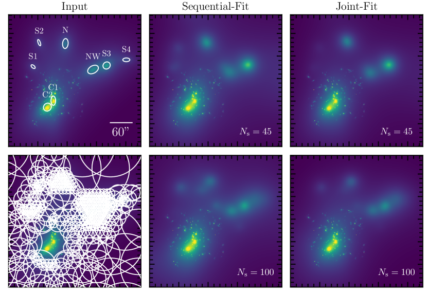
Figure 1: Projected mass maps. Left column: Input simulation, with the large scale potentials shown as white ellipses (top panel), and the potentials of the multiscale grid shown as white circles, which sizes are set to the core radii, $s$, of the potential (bottom panel). Middle Column: Sequential-Fit, with source density $N_{\rm{s}}=45$ sources/arcmin² (top) and $N_{\rm{s}}=100$ sources/arcmin² (bottom). Right Column: Joint-Fit, with source density $N_{\rm{s}}=45$ sources/arcmin² (top) and $N_{\rm{s}}=100$ sources/arcmin² (bottom). The Sequential- and Joint-Fit mass maps are means over a 1000 MCMC samples.

3.2 Lenstool mass reconstructions

We perform two mass reconstructions of this simulated cluster: (1) the Sequential-Fit – we model the strong- and weak-lensing regions successively by first optimizing the parametric model in the cluster core with strong-lensing constraints; then we fix this part to its best-fit values, and optimize the grid model with weak-lensing constraints; (2) the Joint-Fit – we simultaneously optimize the parametric$+$grid models including both strong- and weak-lensing constraints, following the method presented in this paper.

We note that for both models presented in this section the parameters describing the galaxy-scale potentials are fixed to the input values. To test the implications of such choice, we perform a fit with these parameters set as free, and the Joint-Fit does not show any improvement on the recovered values compared to the Sequential-Fit.

3.2.1 Sequential-Fit

Strong lensing modeling.

We first reconstruct the cluster mass distribution following the method described in Jauzac et al. (2015), i.e by modeling successively strong- and weak-lensing regions. Therefore we start by modeling the core of the cluster using strong-lensing constraints only, as if we had no knowledge on the presence of substructures in the outskirts. We reconstruct the mass distribution by optimizing the parameters describing the potentials C1 and C2. As is often done in similar analyses wherein the modeling is focused on the central region of the cluster, we keep the cut radius fixed to $r_{\rm{cut}}=1000\,\rm{kpc}$.

To be able to compare between the two methods we perform this strong-lensing optimization in the source plane. The best-fit values of the model parameters are presented in the middle part of Table 1.

Weak lensing component modeling.

As a second step, we add a set of 353 RBFs to model the outskirts of the cluster. They are located at the nodes of a multi-scale grid. The resolution of the grid traces the mass distribution of the simulated cluster, with higher resolution in the densest region (for more details on the multiscale grid, see for instance Jullo & Kneib, 2009; Jauzac et al., 2012). The resulting grid potentials have core radii varying between $s=11\arcsec-87\arcsec$ (i.e. $50-400\,\rm{kpc}$). We remove the RBFs covering the cluster core, and model this central region with the best-fit values of the parametric model described in the previous paragraph (see Table 1). The grid of RBFs is created in a Lenstool input format using our set of publicly available scripts.

We present the projected mass distribution maps resulting from these two successive models in the middle panel of Fig. 1, and refer to it as the Sequential-Fit. The presented mass maps are the mean maps computed as the average of 1000 MCMC realizations.

3.2.2 Joint-Fit

We now reconstruct the cluster mass distribution by optimizing jointly the parametric and the grid models, with both strong- and weak-lensing constraints. We use the same priors on the free parameters as for the Sequential-Fit, and the same multiscale grid. The best-fit parameters of the large-scale potentials are given in the right panel of Table 1, and the resulting mass map is presented in the right panel of Fig 1. We refer to this mass reconstruction as the Joint-Fit.

3.3 Convergence diagnostics

As we modified the MCMC sampling algorithm for hybrid-Lenstool, we provide in this section a few diagnostics on the convergence of the chains. We use the 10 chains from the Joint-Fit with $N_{\rm s}=45$ sources/arcmin², where each chain was evolved for 100 steps after the burn-in phase.

We first verify the chains have converged by inspecting them visually. We then measure the serial correlation of the chains, and plot the auto-correlation functions (ACF) for each of them, i.e the amount of auto-correlation between the terms of the chain as a function of the lag, and verify that they rapidly decrease, and become consistent with 0 starting at lag $\sim 5$. Finally, we perform a Geweke diagnostic on each chain to check that they have reached a stationary state.

3.4 Comparison of the Sequential-Fit and the Joint-Fit mass reconstructions

To compare the reconstructed mass maps obtained with the different models, we compute the normalized residual maps, defined as $(M_{\rm{model}}-M_{\rm{input}})/M_{\rm{input}}$. We present the resulting maps on Fig. 2 for the Sequential (left panel) and Joint-Fit (right panel), and for source densities $N_{\rm{s}}=45$ sources/arcmin² (top), and $N_{\rm{s}}=100$ sources/arcmin² (bottom). The two models appear to well reproduce the simulated cluster, both in the core and the outskirts. As expected, mass reconstructions with a higher source density are closer to the input, i.e. they are better at detecting lower mass substructures such as S4 and S2, and trace better the true shape of substructures. For the two source densities, the Joint-Fit mass reconstructions have a lower overall bias than the Sequential-Fit reconstructions.

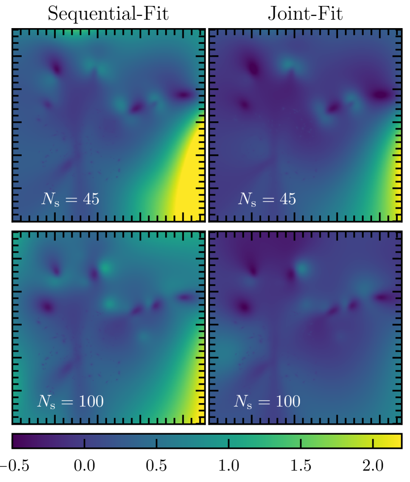
Figure 2: Normalized residual maps for the Sequential-Fit (left) and Joint-Fit (right), and for source density $N_{\rm{s}}=45$ sources/arcmin² (top) and $N_{\rm{s}}=100$ sources/arcmin² (bottom).

Indeed, the best-fit parameters presented in Table 1 indicate that the combined modeling allows us to decrease the bias in the parametric model. When the core of the cluster is first modeled alone as in the Sequential-Fit, the mass in the centre can often be overestimated to compensate for the mass missing in the outskirts. This is reflected in the best-fit values of the parameters $r_{\rm core}$ and/or $\sigma_{0}$ for both C1 and C2 clumps. This gives $M_{\rm{C1}}=(2.00\pm 1.13)\times 10^{13}M_{\sun}$, and $M_{\rm{C2}}=(1.17\pm 1.16)\times 10^{13}M_{\sun}$ for the Sequential-Fit, and $M_{\rm{C1}}=(1.13\pm 0.45)\times 10^{13}M_{\sun}$, and $M_{\rm{C2}}=(1.04\pm 0.45)\times 10^{12}M_{\sun}$ for the Joint-Fit.

To quantify the model deviations from the input simulation, we measure the projected density profiles for each of the models. For each of the 1000 model realizations corresponding to the MCMC samples, we compute a radial density profile by azimuthally averaging the reconstructed mass maps, taking the cluster centre close to the centre of the mass clump, C1. We then average the 1000 profiles, and compute error bars by taking the standard deviation over all 1000 measurements. Figures 3 and 4 show the density profiles for source densities $N=45$, and 100 sources/arcmin² respectively. In both figures, the top panel shows the density profiles, while the bottom panel shows the relative deviations of models as lines and relative errors as shaded areas.

For the two background source number densities, the Sequential-Fit deviates from the simulation by $\sim 2-3\sigma$ on all scales and consistently predicts a higher mass density. As explained before, this is due to the overestimation of the parameters which define the amplitude and size of the central clumps, as this impacts the mass distribution over all scales. Fitting the distribution in the core and in the outskirts self-consistently allows us to avoid this systematic effect. Indeed, Fig. 3 and Fig. 4 show that the Joint-Fit gives a density profile within $1-1.5\sigma$ of the true value over all scales. Finally, the mass density profiles confirm that increasing the source number density allows a better recovery of the shapes of substructures, and produces a smoother mass distribution.

We also compute the integrated mass profiles, and derive the total mass within 1 Mpc, for each model. The mass of the simulated cluster is $M(<1\,\rm{Mpc})=9.02\times 10^{14}M_{\sun}$. As can be inferred from the density profiles, the Sequential-Fit overestimates the total enclosed mass, i.e. $M(<1\,\rm{Mpc})=(11.52\pm 0.68)\times 10^{14}M_{\sun}$ ($(12.43\pm 1.45)\times 10^{14}M_{\sun}$) for $N=45$ (100) sources/arcmin². The Joint-Fit shows a reduced bias on the total mass estimate, and gives values consistent with the true mass: $M(<1\,\rm{Mpc})=(9.43\pm 0.92)\times 10^{14}M_{\sun}$ ($(9.70\pm 0.82)\times 10^{14}M_{\sun}$) for $N=45$ (100) sources/arcmin².

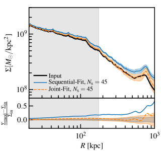
Figure 3: Top panel: Projected mass density profiles of the input simulation (black line), the Sequential-Fit (solid blue line) and the Joint-Fit (dashed orange line) for the source density $N_{\rm{s}}=45$ sources/arcmin². Bottom panel: Relative deviation for the Sequential-Fit (solid blue line) and Joint-Fit (orange dashed line). The shaded regions represent the relative errors for both models. The radial range shown by the grey shaded area corresponds to the strong-lensing region of the simulated cluster.

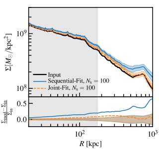
Figure 4: Same as Fig. 3 for source density $N_{\rm{s}}=100$ sources/arcmin².

A commonly used indicator to quantify the goodness of fit for a strong-lensing model is the root-mean-square, noted as rms, i.e. the distance between the observed positions of multiple images and the ones predicted by the best fit model. We compute the best-fit rms values for the different models, and find that the combined modeling with $N_{\rm s}=45$ sources/arcmin² indeed decreases the rms to 0.57″, compared to 0.63″  for the strong-lensing only model of the cluster core. The rms value is further slightly decreased to 0.54″  for the Joint-Fit with $N_{\rm s}=100$, which points that improving the modeling of substructures impacts the quality of fit in the cluster core, in agreement with conclusions from Acebron et al. (2017) analysis. We note that the decrease in rms value can only be considered as a significant estimator of the goodness of fit when comparing between different models of the same cluster, as is the case with our analysis.

The last point we would like to address is the speed of the algorithm. The Joint-Fit mass reconstruction performed with hybrid-Lenstool is significantly slower than the one performed with the regular version of Lenstool. For instance, on a standard laptop, for the models presented here with the source density $N_{\rm s}=45$, the Joint-Fit can be obtained in 15 mn, and the Sequential-Fit in 5 mn (3 mn for the parametric model and 2 mn for the grid). While this result could be expected and is not particularly problematic in this case, this time difference could become more of an issue when modeling very complex systems. In addition, keeping the parameters of the galaxy-scale potentials free further slows down the modeling, and in a larger proportion in the case of the Joint-Fit compared to the Sequential-Fit. Indeed at each step of the optimization, it requires to compute the shear produced by each of the cluster galaxies (which can be hundreds) at the position of each weakly lensed galaxies (which can be thousands). This can be made faster by implementing parallelisation in the computation of the weak-lensing likelihood, as already done for the strong-lensing one.

4 Summary and conclusions

In this paper, we present hybrid-Lenstool, a new method implemented in the publicly available lens reconstruction algorithm Lenstool. It combines strong- and weak-lensing constraints to self-consistently reconstruct the cluster mass distribution at all scales. hybrid-Lenstool combines a parametric model in the cluster core with a free-form grid model in the outskirts. It takes advantage of the complementary strengths of the two types of modeling to recover the shape and amplitude of the mass distribution with high precision.

We tested this new method on a simulated cluster composed of a bi-modal mass distribution in the core and 6 massive substructures in the outskirts. We found that the Joint-Fit modeling recovers well the shape and position of the substructures, and gives a more accurate reconstructed mass density profile for the cluster compared to a Sequential-Fit, where the core and the outskirts of the cluster are modeled separately (method that was used in the past). In addition, the Joint-Fit performs better at predicting the position of multiple images in the cluster core, reducing the rms from 0.63″  to 0.57″.

After demonstrating the power of this new algorithm with simulated data in this method paper, we will present the first application of hybrid-Lenstool to real observations in a forthcoming paper (Niemiec et al., in prep). As mentioned before, the ongoing BUFFALO survey (GO-15117, PIs: Steinhardt & Jauzac, Steinhardt et al., 2020) is extending the HST coverage of the 6 HFF clusters (PI: Lotz, Lotz et al., 2018), and will complement the strong-lensing constraints in the core of these clusters with high resolution weak-lensing data. Combining these datasets, i.e. high resolution constraints both in the strong- and weak-lensing regions of the clusters, with hybrid-Lenstool will produce high-precision models of the mass distribution of the HFF clusters up to $\sim 3/4\,R_{\rm{vir}}$. Higher fidelity mass distributions for cluster lenses are important for utilizing the full potential of clusters to probe dark matter properties and cluster physics, study the distant Universe that they magnify, and be used as cosmological probes, as observed lensing effects are not impacted by the dynamical complexity of clusters.

References

- Acebron et al. (2017) Acebron A., Jullo E., Limousin M., Tilquin A., Giocoli C., Jauzac M., Mahler G., Richard J., 2017, ArXiv e-prints
- Alavi et al. (2016) Alavi A. et al., 2016, ApJ, 832, 56
- Atek et al. (2015) Atek H. et al., 2015, ApJ, 800, 18
- Atek et al. (2018) Atek H., Richard J., Kneib J.-P., Schaerer D., 2018, MNRAS, 479, 5184
- Bahcall (1977) Bahcall N. A., 1977, ARA&A, 15, 505
- Bartelmann & Maturi (2017) Bartelmann M., Maturi M., 2017, Scholarpedia, 12, 32440
- Bartelmann & Schneider (2001) Bartelmann M., Schneider P., 2001, PhysRep, 340, 291
- Bayliss et al. (2019) Bayliss M. B. et al., 2019, Nature Astronomy, 465
- Bayliss et al. (2014) Bayliss M. B., Rigby J. R., Sharon K., Wuyts E., Florian M., Gladders M. D., Johnson T., Oguri M., 2014, ApJ, 790, 144
- Binney & Tremaine (1987) Binney J., Tremaine S., 1987, Galactic dynamics
- Birrer et al. (2019) Birrer S. et al., 2019, MNRAS, 484, 4726
- Bouwens et al. (2017) Bouwens R. J., Illingworth G. D., Oesch P. A., Atek H., Lam D., Stefanon M., 2017, ApJ, 843, 41
- Bradač et al. (2008) Bradač M., Allen S. W., Treu T., Ebeling H., Massey R., Morris R. G., von der Linden A., Applegate D., 2008, ApJ, 687, 959
- Bradač et al. (2006) Bradač M. et al., 2006, ApJ, 652, 937
- Bradač et al. (2005) Bradač M., Schneider P., Lombardi M., Erben T., 2005, Astronomy and Astrophysics, 437, 39
- Bradač et al. (2009) Bradač M. et al., 2009, The Astrophysical Journal, 706, 1201
- Caminha et al. (2016) Caminha G. B. et al., 2016, A&A, 587, A80
- Chisholm et al. (2019) Chisholm J., Rigby J. R., Bayliss M., Berg D. A., Dahle H., Gladders M., Sharon K., 2019, ApJ, 882, 182
- Clowe, Gonzalez & Markevitch (2004) Clowe D., Gonzalez A., Markevitch M., 2004, ApJ, 604, 596
- Coe et al. (2010) Coe D., Benítez N., Broadhurst T., Moustakas L. A., 2010, The Astrophysical Journal, 723, 1678
- Coe et al. (2008) Coe D., Fuselier E., Benítez N., Broadhurst T., Frye B., Ford H., 2008, The Astrophysical Journal, 681, 814
- D’Aloisio & Natarajan (2011) D’Aloisio A., Natarajan P., 2011, MNRAS, 411, 1628
- D’Aloisio, Natarajan & Shapiro (2014) D’Aloisio A., Natarajan P., Shapiro P. R., 2014, MNRAS, 445, 3581
- Diego et al. (2016) Diego J. M. et al., 2016, Monthly Notices of the Royal Astronomical Society, 456, 356
- Diego et al. (2015) Diego J. M., Broadhurst T., Molnar S. M., Lam D., Lim J., 2015, MNRAS, 447, 3130
- Diego et al. (2019) Diego J. M., Hannuksela O. A., Kelly P. L., Pagano G., Broadhurst T., Kim K., Li T. G. F., Smoot G. F., 2019, A&A, 627, A130
- Diego et al. (2018) Diego J. M. et al., 2018, ApJ, 857, 25
- Diego et al. (2005) Diego J. M., Protopapas P., Sandvik H. B., Tegmark M., 2005, Monthly Notices of the Royal Astronomical Society, 360, 477
- Diego et al. (2007) Diego J. M., Tegmark M., Protopapas P., Sand vik H. B., 2007, Monthly Notices of the Royal Astronomical Society, 375, 958
- Eckert et al. (2015) Eckert D. et al., 2015, Nature, 528, 105
- Elíasdóttir et al. (2007) Elíasdóttir Á. et al., 2007, arXiv e-prints, arXiv:0710.5636
- Goobar et al. (2017) Goobar A. et al., 2017, Science, 356, 291
- Harvey, Kneib & Jauzac (2016) Harvey D., Kneib J. P., Jauzac M., 2016, MNRAS, 458, 660
- Harvey et al. (2015) Harvey D., Massey R., Kitching T., Taylor A., Tittley E., 2015, Science, 347, 1462
- Harvey et al. (2017) Harvey D., Robertson A., Massey R., Kneib J.-P., 2017, MNRAS, 464, 3991
- Harvey et al. (2019) Harvey D., Robertson A., Massey R., McCarthy I. G., 2019, MNRAS, 488, 1572
- Hastings (1970) Hastings W., 1970, Biometrika, 57
- Hoekstra et al. (2013) Hoekstra H., Bartelmann M., Dahle H., Israel H., Limousin M., Meneghetti M., 2013, Space Sci.Rev., 177, 75
- Ishigaki et al. (2018) Ishigaki M., Kawamata R., Ouchi M., Oguri M., Shimasaku K., Ono Y., 2018, ApJ, 854, 73
- Jauzac et al. (2018) Jauzac M. et al., 2018, MNRAS, 481, 2901
- Jauzac et al. (2016a) Jauzac M. et al., 2016a, MNRAS, 463, 3876
- Jauzac et al. (2015) Jauzac M. et al., 2015, MNRAS, 446, 4132
- Jauzac et al. (2012) Jauzac M. et al., 2012, MNRAS, 426, 3369
- Jauzac et al. (2016b) Jauzac M. et al., 2016b, MNRAS, 457, 2029
- Johnson, Jones & Neath (2009) Johnson A. A., Jones G. L., Neath R. C., 2009, arXiv e-prints, arXiv:0903.0664
- Johnson et al. (2017) Johnson T. L. et al., 2017, ApJ, 843, L21
- Jullo & Kneib (2009) Jullo E., Kneib J.-P., 2009, MNRAS, 395, 1319
- Jullo et al. (2007) Jullo E., Kneib J.-P., Limousin M., Elíasdóttir Á., Marshall P. J., Verdugo T., 2007, New Journal of Physics, 9, 447
- Jullo et al. (2010) Jullo E., Natarajan P., Kneib J. P., D’Aloisio A., Limousin M., Richard J., Schimd C., 2010, Science, 329, 924
- Jullo et al. (2014) Jullo E., Pires S., Jauzac M., Kneib J.-P., 2014, MNRAS, 437, 3969
- Kawamata et al. (2018) Kawamata R., Ishigaki M., Shimasaku K., Oguri M., Ouchi M., Tanigawa S., 2018, ApJ, 855, 4
- Kelly et al. (2018) Kelly P. L. et al., 2018, Nature Astronomy, 2, 334
- Kelly et al. (2015) Kelly P. L. et al., 2015, Science, 347, 1123
- Kneib et al. (2003) Kneib J.-P. et al., 2003, ApJ, 598, 804
- Kneib & Natarajan (2011) Kneib J.-P., Natarajan P., 2011, A&A Rev., 19, 47
- Lagattuta et al. (2019) Lagattuta D. J. et al., 2019, Monthly Notices of the Royal Astronomical Society, 485, 3738
- Leauthaud et al. (2015) Leauthaud A. et al., 2015, MNRAS, 446, 1874
- Leauthaud et al. (2012) Leauthaud A. et al., 2012, ApJ, 744, 159
- Li et al. (2016) Li R. et al., 2016, MNRAS, 458, 2573
- Liesenborgs, De Rijcke & Dejonghe (2006) Liesenborgs J., De Rijcke S., Dejonghe H., 2006, MNRAS, 367, 1209
- Liesenborgs et al. (2009) Liesenborgs J., de Rijcke S., Dejonghe H., Bekaert P., 2009, MNRAS, 397, 341
- Limousin et al. (2007) Limousin M., Kneib J. P., Bardeau S., Natarajan P., Czoske O., Smail I., Ebeling H., Smith G. P., 2007, A&A, 461, 881
- Lotz et al. (2018) Lotz M., Remus R.-S., Dolag K., Biviano A., Burkert A., 2018, ArXiv e-prints
- Lynds & Petrosian (1986) Lynds R., Petrosian V., 1986, in BAAS, Vol. 18, p. 1014
- Mahler et al. (2018) Mahler G. et al., 2018, MNRAS, 473, 663
- Massey et al. (2018) Massey R. et al., 2018, MNRAS, 477, 669
- Massey et al. (2015) Massey R. et al., 2015, MNRAS, 449, 3393
- Meneghetti et al. (2017) Meneghetti M. et al., 2017, Monthly Notices of the Royal Astronomical Society, 472, 3177
- Merten et al. (2009) Merten J., Cacciato M., Meneghetti M., Mignone C., Bartelmann M., 2009, A&A, 500, 681
- Merten et al. (2011) Merten J. et al., 2011, MNRAS, 417, 333
- Metropolis et al. (1953) Metropolis N., Rosenbluth A. W., Rosenbluth M. N., Teller A. H., Teller E., 1953, J. Chem. Phys., 21, 1087
- Natarajan et al. (2017) Natarajan P. et al., 2017, MNRAS, 468, 1962
- Natarajan & Kneib (1997) Natarajan P., Kneib J.-P., 1997, MNRAS, 287, 833
- Natarajan, Kneib & Smail (2002) Natarajan P., Kneib J.-P., Smail I., 2002, ApJ, 580, L11
- Natarajan et al. (1998) Natarajan P., Kneib J.-P., Smail I., Ellis R. S., 1998, ApJ, 499, 600
- Natarajan et al. (2009) Natarajan P., Kneib J.-P., Smail I., Treu T., Ellis R., Moran S., Limousin M., Czoske O., 2009, ApJ, 693, 970
- Natarajan et al. (2002) Natarajan P., Loeb A., Kneib J.-P., Smail I., 2002, ApJ, 580, L17
- Navarro, Frenk & White (1996) Navarro J. F., Frenk C. S., White S. D. M., 1996, ApJ, 462, 563
- Niemiec et al. (2017) Niemiec A. et al., 2017, MNRAS, 471, 1153
- Oguri (2010) Oguri M., 2010, glafic: Software Package for Analyzing Gravitational Lensing
- Remolina González, Sharon & Mahler (2018) Remolina González J. D., Sharon K., Mahler G., 2018, ApJ, 863, 60
- Richard et al. (2010) Richard J. et al., 2010, MNRAS, 404, 325
- Rigby et al. (2018) Rigby J. R. et al., 2018, AJ, 155, 104
- Rivera-Thorsen et al. (2019) Rivera-Thorsen T. E. et al., 2019, Science, 366, 738
- Rodney et al. (2018) Rodney S. A. et al., 2018, Nature Astronomy, 2, 324
- Rodney et al. (2015) Rodney S. A. et al., 2015, ApJ, 811, 70
- Sendra et al. (2014) Sendra I., Diego J. M., Broadhurst T., Lazkoz R., 2014, Monthly Notices of the Royal Astronomical Society, 437, 2642
- Sharon et al. (2019) Sharon K. et al., 2019, arXiv e-prints, arXiv:1904.05940
- Sharon et al. (2015) Sharon K. et al., 2015, ApJ, 814, 21
- Sifón et al. (2015) Sifón C. et al., 2015, MNRAS, 454, 3938
- Skilling (2004) Skilling J., 2004
- Smith et al. (2019) Smith G. P. et al., 2019, MNRAS, 485, 5180
- Smith et al. (2018) Smith G. P., Jauzac M., Veitch J., Farr W. M., Massey R., Richard J., 2018, MNRAS, 475, 3823
- Soucail et al. (1987) Soucail G., Fort B., Mellier Y., Picat J. P., 1987, A&A, 172, L14
- Soucail et al. (1988) Soucail G., Mellier Y., Fort B., Mathez G., Cailloux M., 1988, A&A, 191, L19
- Steinhardt et al. (2020) Steinhardt C. L. et al., 2020, arXiv e-prints, arXiv:2001.09999
- Suyu et al. (2018) Suyu S. H., Chang T.-C., Courbin F., Okumura T., 2018, Space Sci.Rev., 214, 91
- Teplitz et al. (2000) Teplitz H. I. et al., 2000, ApJ, 533, L65
- Treu et al. (2016) Treu T. et al., 2016, ApJ, 817, 60
- Walsh, Carswell & Weymann (1979) Walsh D., Carswell R. F., Weymann R. J., 1979, Nature, 279, 381
- Wong et al. (2019) Wong K. C. et al., 2019, arXiv e-prints, arXiv:1907.04869
- Zitrin et al. (2012) Zitrin A., Broadhurst T., Bartelmann M., Rephaeli Y., Oguri M., Benítez N., Hao J., Umetsu K., 2012, Monthly Notices of the Royal Astronomical Society, 423, 2308
- Zitrin et al. (2013) Zitrin A. et al., 2013, The Astrophysical Journal, 762, L30