Sun-like stars shed light on solar climate forcing

Abstract

Recently published, precise stellar photometry of 72 Sun-like stars obtained at the Fairborn Observatory between 1993 and 2017 is used to set limits on the solar forcing of Earth’s atmosphere of $\pm 4.5$ W m^-2 since 1750. This compares with the $+2.2\pm 1.1$ W m^-2 IPCC estimate for anthropogenic forcing. Three critical assumptions are made. In decreasing order of importance they are: (a) most of the brightness variations occur within the average time-series length of $\approx 17$ years; (b) the Sun seen from the ecliptic behaves as an ensemble of middle-aged solar-like stars; and (c) narrow-band photometry in the Strömgren $b$ and $y$ bands are linearly proportional to the total solar irradiance. Assumption (a) can best be relaxed and tested by obtaining more photometric data of Sun-like stars, especially those already observed. Eight stars with near-solar parameters have been observed from 1999, and two since 1993. Our work reveals the importance of continuing and expanding ground-based photometry, to complement expensive solar irradiance measurements from space.

1. INTRODUCTION

The influence of the variable total solar irradiance of Earth (TSI) has remained a major uncertainty in our ability to predict quantitatively how the Sun might contribute to climate change (e.g., Lean, 2018; de Wit et al., 2018). Research in this area is active, but is notoriously plagued by difficulties including historically inaccurate (but precise) irradiance measurements from space, the use of extrapolations based upon linear “proxies”, problems of interpreting incomplete stellar datasets, and the general lack of accurate long-term ($>$ decade-long) variability data of the Sun and stars, problems eloquently summarized by Schrijver et al. (2011). For example, the recently measured differences between the last sunspot minimum of 2008 and earlier minima have sparked much debate, new propositions, and further speculation about future and past solar behavior (e.g. Schrijver et al., 2011; Hady, 2013).

In this article we use precise stellar photometry over the past quarter century (Radick et al., 2018) to set limits on the rate at which the Sun might vary over the next few decades. This new approach takes advantage of these multi-decade data to set statistical limits on the variability of Sun-like stars. To proceed, we must make several assumptions. The important assumptions are: (a) variances (integral of power spectra over all frequencies) are not much larger than those sampled over the average time series durations of 17 years; (b) the Sun behaves in a fashion represented by a carefully selected stellar ensemble as observed from Earth, noting that solar radiation is received at Earth in the ecliptic plane, which is tilted just 7^o from the solar equatorial plane; and (c) that the average of the Strömgren $b$ and $y$ filter differential magnitudes is linearly proportional to TSI.

Assumption (b) has been studied empirically by Schatten (1993); Knaack et al. (2001), the more recent work suggesting that (b) is justified to about 6% levels. Assumption (c) is discussed in depth by Radick et al. (2018). All of these assumptions are testable with further measurements and (perhaps) physical models.

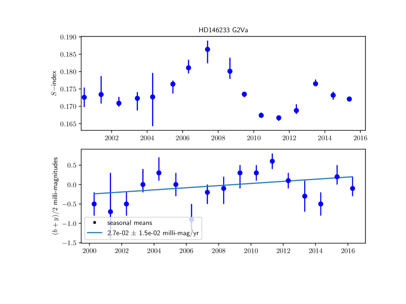
Figure 1.— Seasonally averaged data for the Ca II “S-index” and for the average magnitudes of the Strömgren $b$ plus $y$ filters are shown for the star 18 Sco (HD146233) whose properties are closest to those of the Sun. The straight line in the lower panel shows a least-squares fit of a linear function to the photometric data, with the uncertainties shown as listed in Radick et al. (2018). The gradient is $28\pm 15$ micro-magnitudes per year.

With these assumptions, our careful assessment of uncertainties, along with consistency checks of the stellar time series, we estimate a limit to the secular change of $\pm 19$ milli-magnitudes (0.019 mag) of change in brightness over the standard period of 250 years (Myhre et al., 2013). This amounts to a forcing of $\pm 4.5$ W m^-2 since 1750, and some five times smaller over the next 5 decades.

2. DATA SELECTION AND ANALYSIS

The data analyzed here come primarily from two sources. First, the most precise and stable set of photometric measurements of Sun-like stars (SLS) has been painstakingly acquired by one of us (G.W.H.) using robotic telescopes designed, constructed, and maintained by Louis Boyd at Fairborn Observatory. The photometric data, covering up to 24 years between 1993 and 2017, have been processed and vetted mainly by G.W.H. (described in Henry, 1999). The Fairborn data were recently published by Radick et al. (2018) and made freely available. The second source of data is the Lowell Observatory program on solar and stellar chromospheric activity that produced time series of the magnetically sensitive Ca II line strengths between 1992 and 2016. These measurements were converted to the physical parameter $R^{\prime}_{\mathrm{H}K}$, the ratio of flux in the Ca II lines relative to the stellar luminosity. As a cooperative program with Fairborn, the Lowell observations of the same stars were published together with the photometric results in Radick et al. (2018). We augmented these data with rotation periods and Rossby numbers of these same stars from Table 5.5 of Egeland’s PhD thesis (Egeland, 2017). Further refinement of Egeland’s carefully vetted data were needed to identify true SLS by ensuring consistency with a robust rotation/activity/age relation (Mamajek & Hillenbrand, 2008). Only two stars (HD 86728 and HD 168009) were thus rejected from further analysis. Their periods are from sparse time series of Ca II data over one season from Hempelmann et al., 2016 that seem to us to be overtones of the rotation period. For other stars of particular interest, owing to their similarity to the Sun, we used the rotation/age relationship to estimate ages/rotation rates, and hence the Rossby number $Ro$ (see below and Table 1). These data were used to reject stars on the basis of their different ages, activity levels, and variability.

We initially examined the time series of all 72 stars of Radick et al. (2018) without reference to stellar age, elemental abundances, gravity, effective temperature and other parameters. These data are ideally suited to time-series analysis. All the necessary processing, vetting and calibrations have been done. Unbiased (seasonal) averages of photometric brightness in the standard Strömgren $b$ and $y$ filters were derived, uncertainties quantified, and consistency checks carefully made. Data for our star most similar to the Sun (18 Sco) are shown in Figure 1. It should be noted that each data point for each year consists of many individual measurements, with attention given to a proper quantification of all uncertainties, including those from variations in comparison stars (Radick et al., 2018).

We seek limits on secular (not cyclical) changes in stellar brightness. Therefore, for each star $i$, the gradient of the time series and its formal uncertainty were obtained as shown in Figure 1, and saved as $g_{i}\pm\sigma_{i}$, $i=1\ldots 72$. We then derived the ensemble mean gradient $\langle G(\tau)\rangle$ and its uncertainty $\sigma(\tau)$. Each $g_{i}$ has associated with it the time series duration $\tau_{i}$ from which it was so-derived; $\tau=17$ years is the mean duration of the stellar time series. Cyclical variations that occur in roughly 30% of SLS (Egeland, 2017) will naturally contribute to the gradients derived, depending on the amplitude, phase and duration of the cycles. Longer time series will of course reduce the derived gradients of such stars.

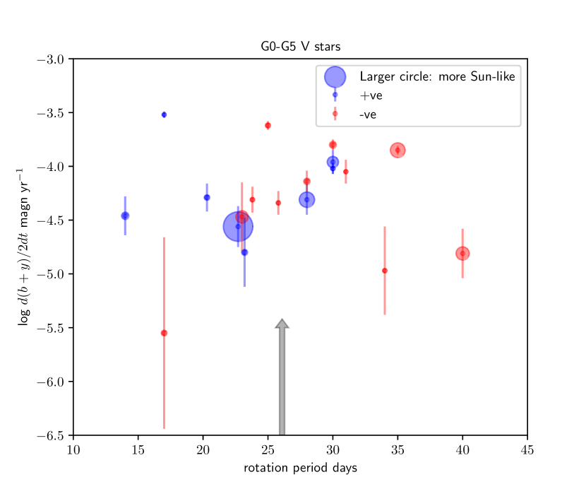
Figure 2.— Computed gradients of the seasonally-averaged $(b+y)/2$ photometric measurements of Radick et al. (2018) are plotted as a function of stellar rotation period. The ordinate is the logarithm of the magnitude change, i.e. $\log_{10}\left(1.086\log_{10}\Delta F/F\right)$ where $F$ is the flux ($2.5\log_{10}e=1.086$). Thus, for $\Delta F/F\ll 1$, the ordinate is proportional to $\log_{10}\Delta F$, i.e. the logarithm of the flux changes. The sizes of the symbols are inversely proportional to the distance metric, the larger the symbol, the more Sun-like is the star (Radick et al., 2018). The solar rotation period is marked with an arrow.

Now we invoke the ergodic hypothesis, i.e. that the Sun’s brightness variations in time are statistically identical to a random sample of SLS (defined below) over a time scale $\tau$ of $17$ years. We can then interpret $\langle G(\tau)\rangle\pm\sigma(\tau)$ as the magnitude of changes in solar brightness averaged over any given epoch covering any contiguous $\tau$ years. The figure of interest here is not $\langle G(\tau)\rangle$ itself of course, but $\sigma(\tau)$.

By invoking this hypothesis, we assume that essentially all of the variance in brightness of SLS occurs within the $\lesssim 17$-year span $\tau_{i}$ of the stellar observations. The value of $\langle G(\tau)\rangle\pm\sigma(\tau)$ so-derived can be strictly applied only to solar data for time spans $\lesssim\tau$. If our strong assumption (a) later turns out to be true, then we can extend this strict limitation to longer periods, for example enabling us to estimate variations in solar TSI since 1750.

The sample of 72 stars was winnowed down on the basis of the “metric” measuring the distance of a given star from the Sun defined by Radick et al. (2018), listed and described in our Table 2. In addition, we required that each star be of luminosity class V and have a well-determined measure of activity (we examined rotation period, Rossby number Ro, age, and $R^{\prime}_{HK}$) from which a more “Sun-like” set of stars was found. The stars that survived all criteria for selection are listed in Table 1.

Table 1 The subset of stars analyzed

HD	Sp.	B-V	age (Gyr)		$p_{rot}$	var.
			low	up	days	type
∗1461	G3VFe0.5	0.68	0.9	3.1	17.0	poor
10307	G1V	0.62	3.5	8.2
13043	G2V	0.62	4.3	7.6	34.0
∗38858	G2V	0.64	3.2	7.5	40.0
42618	G4V	0.64
43587	G0V	0.61	4.45	5.49	20.3	flat
∗50692	G0V	0.6	4.0	6.0	25.0
∗52711	G0V	0.59	4.9	9.7	30.0
∗95128	G1-VFe-0.5	0.61	6.03	6.03	30.0
∗101364	G5	0.65	3.5	3.5	23.0
109358	G0V	0.58	5.3	7.1	28.0
120066	G0V	0.59
126053	G1.5V	0.63	5.49	5.49	35.0	poor?
141004	G0-V	0.6	5.8	6.7	25.8	long
143761	G0+VaFe	0.6	8.5	11.9	17.0	long
146233	G2Va	0.65	3.65	3.75	22.7	good
∗157214	G0V	0.62	4.1	6.6	14.0	irr.
∗159222	G1V	0.62	3.5	6.0	28.0
∗186408	G1.5Vb	0.62	6.7	7.3	23.8	flat
∗186427	G3V	0.66	6.7	7.3	23.2	flat
∗187923	G0V	0.65	8.1	9.5	31.0
∗197076	G5V	0.61	0.2	9.3	30.0

Note. — Upper and lower limit estimates of stellar ages are listed under “low” and “up” in Gyr. The ages are from Egeland (2017), except where marked with an asterisk, where ages are cruder estimates from isochrones in the literature, using HIPPARCOS distances and visible magnitudes. For these stars the rotation-age relations were used to estimate $p_{rot}$ and Ro (Table 2) except when rotation periods were known.

Fortunately, the results depend little on the precise choice of selection parameters. The best result with the smallest dispersion of gradients was found by restricting the sample to stars with the “activity parameter” $\log R^{\prime}_{HK}\leq-4.8$, which is close to the solar value of ${-4.94}$. This final restriction yielded a sample of 22 stars with an ensemble mean gradient

$$\langle G(\tau)\rangle\approx-6{\pm 19}{\rm\ micro-magnitudes\ per\ year.}$$ (1)

The estimate is consistent with a value of zero, as it must be if a large enough number of stars behave independently. The gradients derived from this set of stellar time series are shown in Figure 2, plotted as a function of stellar rotation period. The linear trends extracted are given in Table 2.

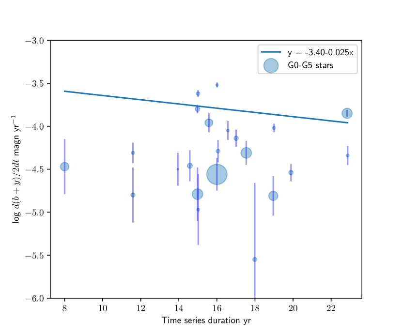
Figure 3.— Secular gradients are shown as a function of time series duration. The solid line shows a linear least-squares fit to the data taking into account the formal error estimates to the fits for each star.

The ensemble mean gradient corresponds to a forcing of the climate by solar irradiation alone of

$$\Delta F(\tau)_{\odot}\approx-1.5{\pm 4.5}{\rm\ W~{}m^{-2}~{}since~{}1750},$$ (2)

where we have used $G=(1.55\pm 0.37)\Delta F/F$ to convert from milli-magnitudes to irradiance changes $\Delta F$ in W m^-2 (Radick et al., 2018) for an average irradiance of $F=1361$ W m^-2. The important figure here is the range of the slope from the uncertainties of $\pm 4.5$ W m^-2. The significance of this estimate is seen when compared with the climate forcing since 1750 due to anthropogenic effects, which is estimated by the IPCC (Myhre et al., 2013) to be

$$\Delta F_{AG}\approx 1.1\ \mathrm{to}\ 3.3{\rm\ W~{}m^{-2}~{}since~{}1750}.$$ (3)

Table 2 Derived stellar properties

HD	dis.	Ro	$\log R^{\prime}_{HK}$	$\tau$	————Gradient————
					$\log g_{i}(\tau)$	sign	$\log\sigma_{i}$
				yr	mag/yr		mag/yr
1461	0.68	1.8	-5.04	17.99	-5.55	$-$	0.89
10307	0.61		-5.01	19.89	-4.54	$+$	0.10
13043	0.92	3.3	-5.01	15.02	-4.97	$-$	0.41
38858	0.29	3.5	-4.89	18.96	-4.81	$-$	0.23
42618	0.25		-4.96	14.98	-4.79	$-$	0.31
43587	0.71	2.6	-4.99	16.06	-4.29	$+$	0.13
50692	0.74	2.84	-4.96	15.01	-3.62	$-$	0.04
52711	0.57	3.6	-4.96	14.98	-3.80	$-$	0.05
95128	0.89	3.0	-5.06	19.0	-4.02	$+$	0.05
101364	0.31	1.9	-4.97	8.0	-4.47	$-$	0.32
109358	0.61	4.9	-4.97	17.01	-4.14	$-$	0.10
120066	1.47		-5.14	13.95	-4.50	$+$	0.19
126053	0.26	3.04	-4.94	22.84	-3.85	$-$	0.04
141004	0.93	2.84	-4.97	22.87	-4.34	$-$	0.11
143761	1.08	1.87	-5.09	16.01	-3.52	$+$	0.03
146233	0.13	1.9	-4.93	16.0	-4.56	$+$	0.19
157214	0.53	1.37	-5.01	14.58	-4.46	$+$	0.18
159222	0.25	2.7	-4.89	17.54	-4.31	$+$	0.14
186408	0.88	1.89	-5.07	11.59	-4.31	$-$	0.12
186427	0.65	1.9	-5.04	11.59	-4.80	$+$	0.32
187923	1.01	2.6	-5.05	16.58	-4.05	$-$	0.11
197076	0.34	3.0	-4.89	15.58	-3.96	$+$	0.11

Note. — “dis.” is the measure of dissimilarity of the star from the Sun (Radick et al., 2018). It is defined by measuring its distance from the Sun in a three-dimensional $M_{V}$, $B-V$ and , $\log R^{\prime}_{HK}$ manifold.

The stars are therefore tantalizingly close to providing useful constraints on magnetically-induced solar irradiance variations, independent of any other measurements or assumptions.

On face value, the uncertainties and shortness of the time series of SLS limit the apparent usefulness of stellar photometry in addressing pressing climate change problems facing humanity (Myhre et al., 2013). However, the present work represents only the first measurements to limit the irradiances of SLS on periods that otherwise require untestable extrapolations (“reconstructions”) or the patching together of different satellite measurements of total solar irradiance by ad-hoc offsets in radiometric calibrations.

The current IPCC estimates of solar forcing (-0.3 to +0.1 W m^-2) (Myhre et al., 2013) are an order of magnitude smaller. However, these numbers have been derived using precisely those extrapolations based upon “proxies” that we are specifically trying to avoid. They are more educated guesses than hard data.

It therefore is important to see how stellar photometry might yield improved results through longer data sets.

• Observing stars over a longer time span will measure more of the low-frequency $(1/\tau_{i})$ components of the power spectrum that contribute to the variances in brightness.

• Depending on the (unknown) amount of power at low frequencies, the increase in lengths of time series may or may not decrease the variances of the measured gradients. In the limit where all the power has been captured in $\tau=17$ years, the slopes and their standard deviations will vary roughly as $1/\tau_{i}$.

• Observing a larger number $N$ of stars will reduce the uncertainties by a factor $\sqrt{N}$.

The second point is illustrated by comparing the statistical stellar behavior against “a reconstruction” with a very large irradiance variation (several W m^-2) since 1750. We examine this below (Section 3). An example of a large linear trend is shown in Figure 4, showing data for HD 126053, which occupies the point near (23,-3.8) in Figure 3. The star is very similar to the Sun ($dis=0.26$); it has been observed for 22 years; yet it has a trend 5 times that of 18 Sco (Figure 1).

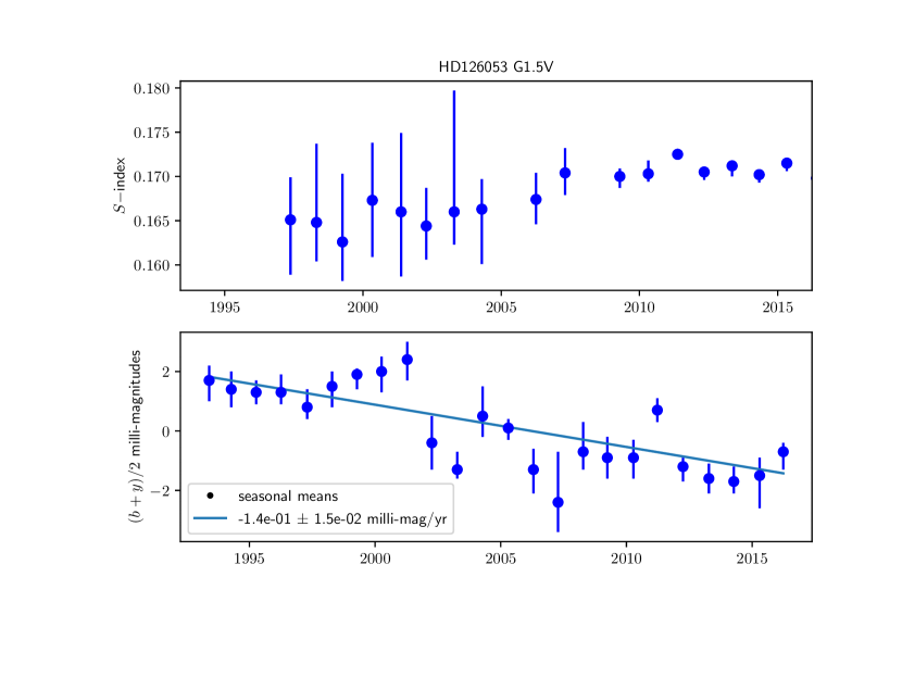
Figure 4.— Data are shown as in Figure 1 for the star HD126053. This star occupies the point (23,-3.8) in Figure 3. It has a well-defined gradient and is very similar to the Sun with a value of $dis=0.26$. The gradient is $140\pm 15$ micro-magnitudes per year, five times that of 18 Sco (Figure 1).

But the essential implication of the length of time series must be important, because a plot of linear trend against length of time series $t_{dur}$ for the sample gives

$$\frac{1}{2}\frac{d}{dt}(b+y)=-3.40-0.50\frac{t_{dur}}{20}$$

with $t_{dur}$ in years (Figure 3).

Additionally, earlier photometric data of one target (HD143761) were published by Lockwood et al. (1997). While these were obtained with a different system at Lowell Observatory having larger uncertainties than those of Radick et al. (2018), they were compared with the same standard star. By assuming that the average of each time series for HD143761 are identical (again, a strong assumption), we can effectively extend the time series from 16 to 32 years (1984-2016). Under the strong assumption, the gradient is reduced from -3.52 (Table 2) to -3.92. Therefore, we can reasonably expect the gradients to decrease with increasing time series duration.

The last bulleted point has a few practical problems, given that society would like information on the role of solar variations as a source of global warming or cooling in the next few decades. First, new time series would build up from year zero, and at least a decade would pass before meaningful statistics could be derived. Second, the selection of good comparison stars is a tedious but important problem, requiring human vetting to achieve reliable results (e.g. Henry, 1999). Lastly, the number of genuinely SLS bright enough to measure with modest (meter-class) telescopes is small. As measured by the number of stars in a meaningful volume of hyper-space similar to the Sun (Radick et al., 1998), considerable work would be needed to identify new, dimmer targets.

There remains the nagging question of whether the Sun is different from other SLS (Gustafsson, 1998). Radick et al. (2018) conclude:

“it may be unusual in two respects: (1) its comparatively smooth, regular activity cycle, and (2) its rather low photometric brightness variation relative to its chromospheric activity level and variation…”

These authors speculate that facular brightening may nearly balance sunspot darkening, explaining the second point. Egeland (2017) pointed out that the Sun has the most regular cycle of all Sun-like stars measured so far.

The question of whether the Sun acts (magnetically) as other SLS is difficult to answer. If all such stars are indeed magnetically similar, it implies that stars have a consistent magnetic variability over time scales of several Gyr (the age range of our sample) to $\sim$100 million years. The latter is close to the uncertainty in ages of older main sequence stars obtained using the best available methods. It is impossible to verify or refute the question for the Sun, even using a cosmogenic proxy record, which presently stretches only 0.01 million years into the past (Wu et al., 2018). Certainly, the most Sun-like of the stars found so far, 18 Sco (HD 146233) has clear differences in metallicity and starspot cycle length. Nevertheless, there is hope that a carefully selected stellar ensemble can represent the activity of the Sun in middle and old age. van Saders et al. (2016) demonstrated that rotation rates of middle-aged and old GV stars converge as a result of weakened magnetic breaking. Unlike younger stars, there is perhaps a good physical reason to believe that magnetic dynamos of older Suns, and their effects, should be similar.

3. TIME SERIES FROM A SOLAR “RECONSTRUCTION”

The limits of our analysis due to the lack of longer time series can be illustrated through a comparison of our results with a “reconstruction” of solar variations with extraordinary and significant forcing of $\approx 6$ W m^-2 from 1600 to 2010 Shapiro et al. (2011). Figure 5 highlights two extended periods of near-monotonic large changes predicted over 15 and 50 years. The first is compatible with several stars (HD 126053, 52711, 50692, 143761; Table 2). The second (50-year) period is compatible with about half of the stars listed.

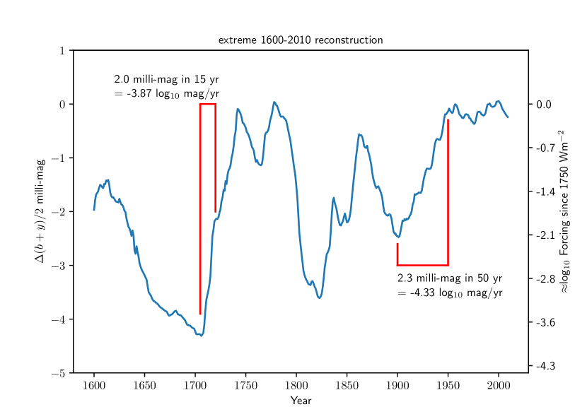
Figure 5.— Variations from a model by Shapiro et al. (2011) are shown, in which variations in radiative forcing since 1750 are of order 3 W m^-2, far larger than the IPCC estimate of –0.30 to +0.10 W m^-2 Myhre et al. (2013). (The relationship between Strömgren magnitudes and irradiance is linear, taken from the model computations. The factor differs from the values adopted in the text, but it is of no consequence for the arguments in the text).

A distribution of the number of stars of a given slope is compared with equivalent distributions extracted from the time series from the reconstruction model in Figure 6. The two distributions (and the third corresponding to a 36-year span of solar observations) are statistically compatible with the same underlying distribution, according to the standard Kolmogorov-Smirnoff test. However, a peak near $10^{-4.5}$ magnitudes per year persists in the reconstructed distribution. The peak arises mostly from the periods of long-term variations, two of which are highlighted in Figure 5.

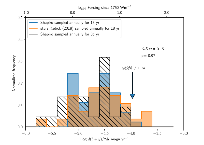
Figure 6.— The distributions of stars according to their derived secular slope ($d(b+y)/2dt$) is shown along with distributions drawn from time-series extracted from the computations. All three distributions are compatible with being drawn from the same underlying distribution according to the Kolmogorov-Smirnoff test. Statistics are shown for the test applied to the two 18-year distributions. (The first parameter is a measure of non-parametric “distance” between two distributions, the second is the probability that they are drawn from the same distribution). Notice that the 36-year calculated distribution moves to the left by about a factor of two.

Our comparison of an (albeit) extreme solar reconstruction with stellar data is a reminder that precise photometry requires patience. It would be unfortunate if the precise photometry performed since 1993 were not followed up with similar data over the next few decades to constrain further long-term solar variability.

4. CONCLUSIONS

Already we have measurements of stellar behavior over periods longer than any direct and stable measure of solar irradiance. (Of all experiments, VIRGO on the SoHO spacecraft has operated almost continuously for 24 years, but it suffers from difficult calibration issues over this period, see Pauluhn et al., 2015). Our limit of $\pm 4.5$ W m^-2 of solar forcing since 1750 hinges on two critical assumptions: first, that the Sun behaves like a member of an ensemble of SLS; second, that the stellar sample has measured essentially all of the variance in the seasonal stellar time series, from a frequency of $1/17$ years^-1 to 2 years (Nyqvist limit). According to current understanding these changes occur because of magnetic activity. Certainly we can expect more power to be present on longer time scales owing to magnetic variations among the stars. But the question is, how much? In this regard we note that the length of time series is only 0.8 of the solar magnetic activity cycle. Thus we might expect some of the larger gradients to begin dropping out with additional data for those stars that are known to be cycling (or perhaps irregular, see Egeland, 2017), as the linear trends become replaced by cycles that might return to the same brightness, given two or more complete cycles.

Only by observing these stars for longer periods can we set tighter limits on the ensemble’s typical behavior (Figure 6). It is therefore of great importance to find a way to continue the observational program pioneered at Fairborn Observatory. With the advent of remotely controlled automated telescopes, a cost-effective way to continue these measurements is surely within reach. The challenges to obtain funding for such work remain to be addressed, as the Fairborn observatory work cannot continue for long without investment in people as well as funding.

We have made some use of rotation-age relationships (Mamajek & Hillenbrand, 2008); additional work to determine precise rotation periods would be useful for specific stars. Lastly, we have proposed earlier (Judge & Egeland, 2015) that the solar $b$ and $y$ colors be monitored by placing an inert sphere in geosynchronous orbit and observing it in the same way as the stars for the lifetime of the sphere.

Acknowledgments We are grateful to Louis Boyd for his many years of devotion at Fairborn Observatory. Without his work, results such as those presented here would remain out of reach to all. Giuliana de Toma provided helpful comments on the manuscript. G.W.H. acknowledges long-term support from NASA, NSF, Tennessee State University, and the State of Tennessee through its Centers of Excellence program. The National Center for Atmospheric Research is funded by the National Science Foundation.

References

- de Wit et al. (2018) de Wit, T. D., Funke, B., Haberreiter, M., & Matthes, K. 2018, Eos, 99
- Egeland (2017) Egeland, R. 2017, PhD thesis, Montana State University, Bozeman, Montana, USA
- Gustafsson (1998) Gustafsson, B. 1998, in Solar Composition and Its Evolution – From Core to Corona, ed. C. Fröhlich, M. C. E. Huber, S. K. Solanki, & R. von Steiger, 419
- Hady (2013) Hady, A. A. 2013, Journal of Advanced Research, 4, 209
- Hempelmann et al. (2016) Hempelmann, A., Mittag, M., Gonzalez-Perez, J. N., et al. 2016, A & A, 586, A14
- Henry (1999) Henry, G. W. 1999, PASP, 111, 845
- Judge & Egeland (2015) Judge, P. G., & Egeland, R. 2015, MNRAS, 448, L90
- Knaack et al. (2001) Knaack, R., Fligge, M., Solanki, S. K., & Unruh, Y. C. 2001, A&A, 376, 1080
- Lean (2018) Lean, J. L. 2018, Earth and Space Science, 5, 133
- Lockwood et al. (1997) Lockwood, G. W., Skiff, B. A., & Radick, R. R. 1997, ApJ, 485, 789
- Mamajek & Hillenbrand (2008) Mamajek, E. E., & Hillenbrand, L. A. 2008, ApJ, 687, 1264
- Myhre et al. (2013) Myhre, G., Shindell, D., Bréon, F.-M., et al. 2013, in Climate Change 2013 (Cambridge, United Kingdom and New York, NY, USA: Cambridge University Press)
- Pauluhn et al. (2015) Pauluhn, A., Huber, M. C. E., Smith, P. L., & Colina, L. 2015, A&A Rev., 24, 3
- Radick et al. (2018) Radick, R. R., Lockwood, G. W., Henry, G. W., Hall, J. C., & Pevtsov, A. A. 2018, ApJ, 855, 75
- Radick et al. (1998) Radick, R. R., Lockwood, G. W., Skiff, B. A., & Baliunas, S. L. 1998, ApJS, 118, 239
- Schatten (1993) Schatten, K. H. 1993, J. Geophys. Res., 98, 18907
- Schrijver et al. (2011) Schrijver, C. J., Livingston, W. C., Woods, T. N., & Mewaldt, R. A. 2011, Geophys. Res. Lett., 38, L06701
- Shapiro et al. (2011) Shapiro, A. I., Schmutz, W., Rozanov, E., et al. 2011, A&A, 529, A67
- van Saders et al. (2016) van Saders, J. L., Ceillier, T., Metcalfe, T. S., et al. 2016, Nature, 529, 181
- Wu et al. (2018) Wu, C. J., Krivova, N. A., Solanki, S. K., & Usoskin, I. G. 2018, A&A, 620, A120