Imbalanced classification: a paradigm-based review

Abstract

A common issue for classification in scientific research and industry is the existence of imbalanced classes. When sample sizes of different classes are imbalanced in training data, naively implementing a classification method often leads to unsatisfactory prediction results on test data. Multiple resampling techniques have been proposed to address the class imbalance issues. Yet, there is no general guidance on when to use each technique. In this article, we provide a paradigm-based review of the common resampling techniques for binary classification under imbalanced class sizes. The paradigms we consider include the classical paradigm that minimizes the overall classification error, the cost-sensitive learning paradigm that minimizes a cost-adjusted weighted type I and type II errors, and the Neyman-Pearson paradigm that minimizes the type II error subject to a type I error constraint. Under each paradigm, we investigate the combination of the resampling techniques and a few state-of-the-art classification methods. For each pair of resampling techniques and classification methods, we use simulation studies and a real data set on credit card fraud to study the performance under different evaluation metrics. From these extensive numerical experiments, we demonstrate under each classification paradigm, the complex dynamics among resampling techniques, base classification methods, evaluation metrics, and imbalance ratios. We also summarize a few takeaway messages regarding the choices of resampling techniques and base classification methods, which could be helpful for practitioners.

Keywords: Binary classification, Imbalanced data, Resampling methods, Imbalance ratio, Classical Classification (CC) paradigm, Neyman-Pearson (NP) paradigm, Cost-Sensitive (CS) learning paradigm.

1 Introduction

Classification is a widely studied type of supervised learning problem with extensive applications. A myriad of classification methods (e.g., logistic regression, support vector machines, random forest, neural networks, boosting), which we refer to as the base classification methods in this paper, have been developed to deal with different distributions of data (Kotsiantis et al., 2007). However, in the case where the classes are of different sizes (i.e., the imbalanced classification scenario), naively applying the existing methods could lead to undesirable results. Some prominent applications include defect detection (Arnqvist et al., 2021), medical diagnosis (Chen, 2016), fraud detection (Wei et al., 2013), spam email filtering (Youn and McLeod, 2007), text categorization (Zheng et al., 2004), oil spills detection in satellite radar images (Kubat et al., 1998), land use classification (Ranneby and Yu, 2011). To address the class size imbalance scenario, there has been extensive research on developing different methods (Sun et al., 2009; López et al., 2013; Guo et al., 2017). Some popular tools include resampling techniques (López et al., 2013; Alahmari, 2020; Anis et al., 2020), direct methods (Lin et al., 2002; Ling et al., 2004; Zhou and Liu, 2005; Sun et al., 2007; Qiao et al., 2010), post-processing methods (Castro and Braga, 2013), as well as different combinations of these tools. The most common and understandable class of approaches is resampling techniques. However, there lacks a consensus about when and how to use them.

In this work, we aim to provide some guidelines on using resampling techniques for imbalanced binary classification. We first disentangle the general claims of undesirability in classification results under imbalanced classes, via listing a few common paradigms and evaluation metrics. To decide which resampling technique to use, we need to be clear on the paradigms as well as the preferred evaluation metrics. Sometimes, the chosen paradigm and the evaluation metric are not compatible, which makes the problem unsolvable by any technique. When they are, we will show that the optimal resampling technique depends on both the paradigm and the base classification method.

There are different degrees of data imbalance. We characterize this degree by the imbalance ratio (IR) (García et al., 2012b), which is the ratio of the sample size of the majority class and that of the minority class. In real applications, IR can range from $1$ to more than $1,000$. For instance, a rare disease occurs only in 0.1% of the human population (Beaulieu et al., 2014). We will show that different IRs might demand different combinations of resampling techniques and base classification methods.

This review conducts extensive simulation experiments as well as a real data set on credit card fraud to concretely illustrate the dynamics among data distributions, IR, base classification methods, and resampling techniques. This is the first time that such dynamics are explicitly examined. To the best of our knowledge, this is also the first time that a review paper uses running simulation examples to demonstrate the advantages and disadvantages of the reviewed methods. Through simulation and real data analysis, we give practitioners a look into the complicated nature of the imbalanced data problem in classification, even if we narrow our search to the resampling techniques only. For important applications where data distributions can be approximately simulated, practitioners are encouraged to mimic our simulation studies and properly evaluate the combinations of resampling techniques and base classification methods. In the end, we summarize a few takeaway messages regarding the choices of resampling techniques and base classification methods, which could be helpful for practitioners.

The rest of the review is organized as follows. In Section 2, we describe three classification paradigms and discuss their corresponding objectives. Then, we introduce a matrix of classification algorithms as pairs of resampling techniques and the base classification methods in Section 3. Section 4 provides a list of commonly used evaluation metrics for imbalanced classification. In Sections 5 and 6, we conduct a systematic simulation study and a real data analysis to evaluate the performance of different combinations of resampling techniques and base classification methods, under different paradigms, data distributions, and IRs, in terms of various evaluation metrics. We conclude the review with a short discussion in Section 7.

2 Three Classification Paradigms

In this section, we review three classification paradigms that are defined by different objective functions. Concretely, we consider the Classical Classification (CC) paradigm that minimizes the overall classification error (Section 2.1), the Cost-Sensitive (CS) learning paradigm that minimizes the cost-adjusted weighted type I and type II errors (Section 2.2), and the Neyman-Pearson (NP) paradigm that minimizes the type II error subject to a type I error constraint (Section 2.3).

Assume $X\in\mathcal{X}\subset{\mbox{\boldmath$R$}}^{d}$ is a random vector of $d$ features, and $Y\in\{0,1\}$ is the class label. Let ${\rm I}\kern-1.79993pt{\rm P}(Y=0)=\pi_{0}$ and ${\rm I}\kern-1.79993pt{\rm P}(Y=1)=\pi_{1}=1-\pi_{0}$. Throughout the article, we label the minority class as 0 and the majority class as 1 (i.e., $\pi_{0}\leq\pi_{1}$). Also, for language consistency, we call class 0 the negative class and class 1 the positive class. Please note that the minority class might be referred to as “positive” in medical applications.

2.1 Classical Classification paradigm

A classifier is defined as $\phi:\mathcal{X}\rightarrow\{0,1\}$, which is a mapping from the feature space to the label space. The overall classification error (risk) is naturally defined as $R(\phi)={\rm I}\kern-1.79993pt{\rm E}[{\rm 1}\kern-2.40005pt{\rm I}(\phi(X)\neq Y)]={\rm I}\kern-1.79993pt{\rm P}(\phi(X)\neq Y)$, where ${\rm 1}\kern-2.40005pt{\rm I}(\cdot)$ is the indicator function. In binary classification, most existing classification methods focus on the minimization of the overall classification error (risk) (Hastie et al., 2009; James et al., 2013). In this article, this paradigm is referred to as Classical Classification (CC) Paradigm. Under this paradigm, the CC oracle $\phi^{*}$ is a classifier that minimizes the population risk; that is,

$$\phi^{*}=\operatorname*{arg\,min}_{\phi}R(\phi)\,.$$

It is well known that $\phi^{*}={\rm 1}\kern-2.40005pt{\rm I}(\eta(x)>1/2)$, where $\eta(x)={\rm I}\kern-1.79993pt{\rm E}(Y|X=x)$ is the regression function (Koltchinskii, 2011). In practice, we construct a classifier $\hat{\phi}$ based on finite sample $\{(X_{i},Y_{i}),i=1,\cdots,n\}$ using some classification method.

Popular the CC paradigm is, it may not be the ideal choice when the class sizes are imbalanced. By the law of total probability, we decompose the overall classification error as a weighted sum of type I and II errors, that is,

$$R(\phi)=\pi_{0}R_{0}(\phi)+\pi_{1}R_{1}(\phi)\,,$$

where $R_{0}(\phi)={\rm I}\kern-1.79993pt{\rm P}(\phi(X)\neq Y|Y=0)$ denotes the (population) type I error (the conditional probability of misclassifying a class 0 observation as class 1); and $R_{1}(\phi)={\rm I}\kern-1.79993pt{\rm P}(\phi(X)\neq Y|Y=1)$ denotes the (population) type II error (the conditional probability of misclassifying a class 1 observation as class 0). However, in many practical applications, we may want to treat type I and II errors differently under two common scenarios. One is the asymmetric error importance scenario. In this scenario, making one type of error (e.g., type I error) is more serious than making the other type of error (e.g., type II error). For instance, in severe disease diagnosis, misclassifying a diseased patient as healthy could lead to missing the optimal treatment window while misclassifying a healthy patient as diseased can lead to patient anxiety and incur additional medical costs. The other is the imbalanced class proportion scenario. Under this scenario, $\pi_{0}$ is much smaller than $\pi_{1}$, and minimizing the overall classification error could sometimes result in a larger type I error. For applications that fit these two scenarios, the overall classification error may not be the optimal choice to serve the users’ purpose, either as an optimization criterion or as an evaluation metric. Next, we will introduce two other paradigms that have been used the address the asymmetric error importance and imbalanced class proportion issues.

2.2 Cost-Sensitive learning paradigm

In the asymmetric error importance and imbalanced class proportion scenarios introduced at the end of Section 2.1, the cost of type I error is usually higher than that of type II error. For example, in spam email filtering, the cost of misclassifying a regular email as spam is much higher than the cost of misclassifying spam as a regular email. A popular approach to incorporate different costs for these two types of errors is the Cost-Sensitive (CS) learning paradigm (Elkan, 2001; Zadrozny et al., 2003). Let $C(\phi(X),Y)$ being the cost function for classifier $\phi$ at observation pair $(X,Y)$. Let $C_{0}=C(1,0)$ and $C_{1}=C(0,1)$ being the costs of type I and II errors, respectively. For the correct classification result, we have $C(0,0)=C(1,1)=0$. Then, CS learning minimizes the expected misclassification cost (Kuhn and Johnson, 2013):

$$R_{c}(\phi) ={\rm I}\kern-1.79993pt{\rm E}C(\phi(X),Y)$$

$$=C_{0}{\rm I}\kern-1.79993pt{\rm P}(\phi(X)=1,Y=0)+C_{1}{\rm I}\kern-1.79993pt{\rm P}(\phi(X)=0,Y=1)$$

$$=C_{0}{\rm I}\kern-1.79993pt{\rm P}(\phi(X)=1|Y=0){\rm I}\kern-1.79993pt{\rm P}(Y=0)+C_{1}{\rm I}\kern-1.79993pt{\rm P}(\phi(X)=0|Y=1){\rm I}\kern-1.79993pt{\rm P}(Y=1)$$

$$=C_{0}\pi_{0}R_{0}(\phi)+C_{1}\pi_{1}R_{1}(\phi)\,.$$

There are primarily two types of approaches in the literature on CS learning. The first type is called direct methods, which builds a cost-sensitive learning classifier by incorporating the different misclassification costs into the training process of the base classification method. For instance, there has been much work on CS decision tree (Ling et al., 2004; Bradford et al., 1998; Turney, 1994), CS boosting (Sun et al., 2007; Wang and Japkowicz, 2010; López et al., 2015), CS SVM (Qiao and Liu, 2009), and CS neural network (Zhou and Liu, 2005). The second type is usually referred to as postprocessing methods, in such a way that we adjust the decision threshold with the base classification algorithm unmodified. An example of this can be found in Domingos (1999). Some additional references on cost-sensitive learning include López et al. (2012, 2013); Guo et al. (2017); Voigt et al. (2014); Zhang et al. (2016); Zou et al. (2016).

In this review, we focus on the postprocessing methods as it combines well with any existing base classification algorithm without the need to change its internal mechanism, which is also better understood among practitioners. In addition, it serves the purpose of making an informative comparison among different learning paradigms across different classification methods. On the population level, with the knowledge of $C_{0}$ and $C_{1}$, the CS oracle is

$$\phi_{c}^{*}=\operatorname*{arg\,min}_{\phi}R_{c}(\phi)={\rm 1}\kern-2.40005pt{\rm I}\left(\eta(x)>\frac{C_{0}}{C_{0}+C_{1}}\right),$$

which reduces to the CC oracle $\phi^{*}$ when $C_{0}=C_{1}$.

Although CS learning has its merits on the control of asymmetric errors, its drawback is also apparent because it is sometimes difficult or immoral to assign the values of costs $C_{0}$ and $C_{1}$. In most applications, including the severe disease classification, these costs are unknown and cannot be easily provided by experts. One way to extricate from this dilemma is to set the majority class misclassification cost $C_{1}=1$ and the minority class misclassification cost $C_{0}=\pi_{1}/\pi_{0}$ (Castro and Braga, 2013).

2.3 Neyman-Pearson paradigm

Besides requiring the knowledge of costs for different misclassification errors, the CS learning paradigm does not provide an explicit probabilistic control on type I error under a pre-specified level. Even if the practitioner tunes the empirical type I error equal to the pre-specified level, the population-level type I error still has a non-trivial chance of exceeding this level (Tong, Feng, and Zhao, 2016, 2018). To deal with this issue, another emerging statistical framework to control asymmetric error is called Neyman-Pearson (NP) paradigm (Cannon et al., 2002; Rigollet and Tong, 2011; Tong, 2013; Tong et al., 2016, 2018), which aims to minimize type II error $R_{1}(\phi)$ while controlling type I error $R_{0}(\phi)$ under a desirable level. The corresponding NP oracle is

$$\phi_{\alpha}^{*}=\operatorname*{arg\,min}_{\phi:R_{0}(\phi)\leq\alpha}R_{1}(\phi)\,,$$

where $\alpha$ is a targeted upper bound for type I error. It can be shown that $\phi^{*}_{\alpha}(\cdot)={\rm 1}\kern-2.40005pt{\rm I}(\eta(\cdot)>D^{*}_{\alpha})$ for some properly chosen $D^{*}_{\alpha}$. Unlike $1/2$ or $C_{0}/(C_{0}+C_{1})$, $D^{*}_{\alpha}$ is not known unless one has access to the distribution information. Tong et al. (2018) proposed an umbrella algorithm for NP classification, which adapts existing scoring-type classification methods (e.g., logistic regression, support vector machines, random forest) by choosing an order-statistics based thresholding level so that the resulting classifier has type I error bounded from above by $\alpha$ with high probability. This thresholding mechanism, along with the thresholds $1/2$ and $C_{0}/(C_{0}+C_{1})$ for CC and CS paradigms respectively, will be systematically studied in combination with several state-of-the-art base classification methods in numerical studies.

2.4 A summary of three classification paradigms

For readers’ convenience, we summarize the three classification paradigms with their corresponding objectives and oracle classifiers in Table 1.

Table 1: Three types of classification paradigms in binary classification.

Paradigm	Objective	Oracle Classfier
Classical	Minimize the overall classification error	$\phi^{*}=\operatorname*{arg\,min}_{\phi}R(\phi)$
Cost-Sensitive	Minimize the expected misclassification cost	$\phi_{c}^{*}=\operatorname*{arg\,min}_{\phi}R_{c}(\phi)$
Neyman-Pearson	Minimize type II error while controlling	$\phi_{\alpha}^{*}=\operatorname*{arg\,min}\limits_{\phi:R_{0}(\phi)\leq\alpha}R_{1}(\phi)$
	type I error under $\alpha$

3 A Matrix of Algorithms for Imbalanced Classification

In this section, we introduce a matrix of algorithms for imbalanced classification, which consists of combinations of resampling techniques and base classification methods.

To fix idea, assume among the $n$ observation pairs $\{(X_{i},Y_{i}),i=1,\cdots,n\}$, there are $n_{0}$ observations with $Y_{i}=0$ (the minority class) and $n_{1}$ observations with $Y_{i}=1$ (the majority class). Then, the imbalance ratio IR = $n_{1}/n_{0}$.

3.1 Resampling techniques

To address the imbalanced classification problem under one of the three classification paradigms described in Section 2, resampling techniques are often used to create a new training dataset by balancing the number of data points in the minority and majority classes in order to alleviate the effect of class size imbalance in the process of classification. López et al. (2013) pointed out that about one-third of their reviewed papers have used resampling techniques. They are usually divided into three categories: undersampling, oversampling, and hybrid methods.

The undersampling methods directly discard a subset of observations of the majority class. It includes two main versions: the cluster-based undersampling and random undersampling (Yen and Lee, 2009; Kumar et al., 2014; Sun et al., 2015; Guo et al., 2017). In the cluster-based undersampling, a clustering algorithm is applied to cluster the majority class such that the number of clusters is equal to that of the data points in the minority class (i.e., $n_{0}$ clusters), and then one point is randomly selected from each cluster. Nevertheless, the clustering process could be quite slow when $n_{1}$ is large. Random undersampling is a simpler and more efficient approach, which randomly eliminates the data points from the majority class to make it of size $n_{0}$. By undersampling, the processed training data set is a combination of $n_{0}$ randomly chosen data points from the majority class and all ($n_{0}$) data points from the minority class. However, undersampling may lead to loss of information as a large portion of the data from the majority class is discarded.

The oversampling method, on the other hand, increases the number of data points in the minority class from $n_{0}$ to $n_{1}$ while keeping the observations from the majority class intact. The leading two approaches are random oversampling and SMOTE (Han et al., 2005; He et al., 2008; García et al., 2012a; Beaulieu et al., 2014; Nekooeimehr and Lai-Yuen, 2016). Random oversampling, as a counterpart of random undersampling, is perhaps the most straightforward approach to duplicate the data points of minority class randomly. One version of the approach samples $n_{1}-n_{0}$ observations with replacement from the minority class and add them to the new training set. The approach SMOTE is the acronym for the “Synthetic Minority Over-sampling Technique” proposed by Chawla et al. (2002). It generates $n_{1}-n_{0}$ new synthetic data points for the minority class by interpolating pairs of $k$ nearest neighbors. We review the details of SMOTE in Algorithm 1. Compared with undersampling, oversampling methods usually require longer training time and could cause over-fitting. A popular extension of SMOTE is the Borderline-SMOTE (BLSMOTE) (Han et al., 2005), which only oversamples the minority observations near the borderline and the essential step to generate the data point is similar to the SMOTE algorithm in Algorithm 1 (see Han et al. (2005) for a detailed description for BLSMOTE).

For any data point of minority class $X_{i}=(X_{i1},X_{i2},\ldots,X_{id})^{\top}$, the multiple $N=IR-1$, number of nearest neighbors $K$

Step 1: Find the $K$ nearest neighbor points of $X_{i}$ in the minority class: $X_{i_{1}},\ldots,X_{i_{k}}$;

Step 2: for $j=1:N$ do

       randomly choose one of the $K$ nearest neighbor points: $X_{i_{j}}=(X_{i_{j}1},X_{i_{j}2},\ldots,X_{i_{j}d})^{\top}$;

       generate a random number $r_{s}\sim Unif[0,1]$;

       generate the synthetic data point for the minority class as $X_{j}^{*}=(X_{j1}^{*},X_{j2}^{*},\ldots,X_{jd}^{*})^{\top}$, where $X_{js}^{*}=X_{is}+r_{s}*(X_{i_{j}s}-X_{is})$, $s=1,\ldots,d$.

end for

Return $X_{1}^{*},\ldots,X_{N}^{*}$ as new synthetic data points.

Algorithm 1 SMOTE (Chawla et al., 2002)

The hybrid method is just a combination of undersampling and oversampling methods (Cao et al., 2014; Cateni et al., 2014; Díez-Pastor et al., 2015; Sáez et al., 2015). It simultaneously decreases the number of data points from the majority class and increases the number of data points from the minority class to $n_{h}$, where the above described undersampling and oversampling methods can be used. The hybrid method could serve as an option that balances the goodness of fit, computational cost as well as robustness of the classifier.

3.2 Classification methods

Using any of the resampling methods, we will arrive at a new training dataset that has balanced classes. Naturally, we can apply any existing base classification method on this new dataset coupled with one of the paradigms described in Section 2.

Many classification methods have been extensively studied. The well-known ones include decision trees (DT) (Safavian and Landgrebe, 1991), $k$-nearest neighbors (KNN) (Altman, 1992), Linear discriminant analysis (LDA) (McLachlan, 2004), logistic regression (LR) (Nelder and Wedderburn, 1972), naïve bayes (NB) (Rish et al., 2001), neural network (NN) (Rumelhart et al., 1985), random forest (RF) (Breiman, 2001), support vector machine (SVM) (Cortes and Vapnik, 1995), and XGBoost (XGB) (Chen and Guestrin, 2016), among others.

To learn more about these methods, we refer the readers to a review of classification methods (Kotsiantis et al., 2007) and a book on statistical learning (Hastie et al., 2009).

3.3 A summary of the matrix of algorithms

In numerical studies, we consider a matrix of classification algorithms shown in Figure 1, as combinations of resampling techniques described in Section 3.1 and four (out of many) state-of-the-art classification methods described in Section 3.2.

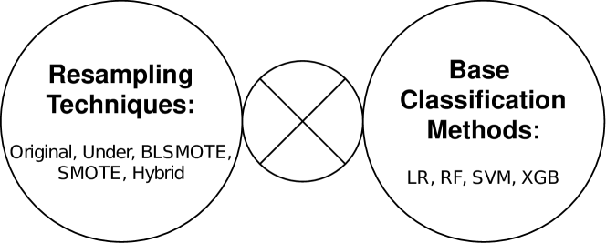
Figure 1: A summary of the matrix of algorithms.

In Figure 1, “Original” refers to no resampling, “Under” refers to random undersampling and “Hybrid” refers to a hybrid of random undersampling and SMOTE. Note here we chose random undersampling, SMOTE, and BLSMOTE as representatives of undersampling and oversampling methods due to their popularity among practitioners. The readers can easily study other types of resampling technique and classification method combinations by adapting the companion code from this review.

In the numerical studies, we will conduct a comparative study on those $20$ combinations described in Figure 1 under each of the three paradigms introduced in Section 2 with the IR varying from $1$ to $128$, in terms of different evaluation metrics which will be introduced in the next section. A flowchart demonstrating our imbalanced classification system can be found in Figure 2.

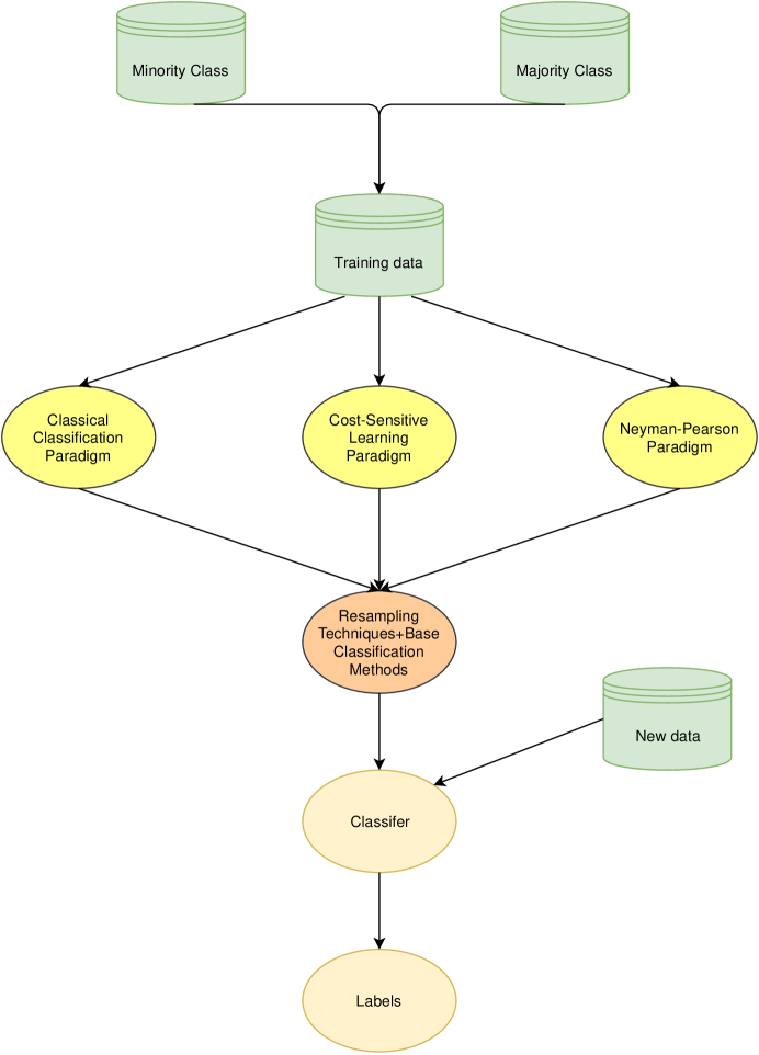
Figure 2: A flow chart for imbalanced classification with a paradigm-oriented view.

4 Evaluation Metrics

In this section, we will review several popular evaluation metrics to compare the performance of different classification algorithms.

For a given classifier, suppose that it classifies the $i$-th observation $X_{i}$ to $\hat{Y}_{i}$ ($Y_{i}$ denotes the true label). Then, the classification results can be summarized into the four terms: True Positives $\mbox{TP}=\sum_{i=1}^{n}{\rm 1}\kern-2.40005pt{\rm I}(Y_{i}=1,\hat{Y}_{i}=1)$, False Positives $\mbox{FP}=\sum_{i=1}^{n}{\rm 1}\kern-2.40005pt{\rm I}(Y_{i}=0,\hat{Y}_{i}=1)$, False Negatives $\mbox{FN}=\sum_{i=1}^{n}{\rm 1}\kern-2.40005pt{\rm I}(Y_{i}=1,\hat{Y}_{i}=0)$, and True Negatives $\mbox{TN}=\sum_{i=1}^{n}{\rm 1}\kern-2.40005pt{\rm I}(Y_{i}=0,\hat{Y}_{i}=0)$. These four terms are usually summarized in the so-called confusion matrix (Table 2).

Table 2: Confusion matrix for a two-class problem.

	Predicted Class 0	Predicted Class 1
True Class 0	TN	FP
True Class 1	FN	TP

Note that in Table 2, the class 0 is being regarded as the “negative class”. In practice, sometimes we may need to set class 0 as the “positive class”.

Then, the empirical risk can be denoted as

$$\hat{R}=\hat{\pi}_{0}\hat{R}_{0}+\hat{\pi}_{1}\hat{R}_{1}=\frac{FP+FN}{TP+FP+TN+FN}\,,$$

where $\hat{\pi}_{0}=(TN+FP)/(TP+FP+TN+FN)$, $\hat{\pi}_{1}=(FN+TP)/(TP+FP+TN+FN)$ are the empirical proportions of Class 0 and 1; $\hat{R}_{0}$ and $\hat{R}_{1}$ are the empirical type I and II errors, respectively, that is,

$$\hat{R}_{0}=\frac{FP}{TN+FP},\ \ \hat{R}_{1}=\frac{FN}{FN+TP}\,.$$

Similarly, for given costs $C_{0}$ and $C_{1}$, the empirical misclassification cost is expressed as

$$\hat{R}_{c}=C_{0}\hat{\pi}_{0}\hat{R}_{0}+C_{1}\hat{\pi}_{1}\hat{R}_{1}\,.$$

Another popular synthetic metric in the imbalanced classification literature is the $F$-score (also $F_{1}$-score or $F$-measure, (Bradley, 1997)) for class 0, which is the harmonic mean of Precision and Recall: where $Precision_{0}=TN/(TN+FN)$ and $Recall_{0}=TN/(TN+FP)$. Similarly, we can also define $F$-score for class 1 as

$$F\mbox{-score (class 1)}=\frac{2}{Precision_{1}^{-1}+Recall_{1}^{-1}}\,,$$

where $Precision_{1}=TP/(TP+FP)$ and $Recall_{1}=TP/(TP+FN)$. Here, we set $F\mbox{-score (class 0)}$ or $F\mbox{-score (class 1)}$ to 0 if the corresponding precision or recall is undefined or equal to 0.

When the parameter in a classification method (e.g., the threshold of scoring functions) is varied, we usually get different trade-offs between type I and type II errors. A popular tool to visualize these trade-offs is the Receiver Operating Characteristic (ROC) curve (Bradley, 1997; Huang and Ling, 2005). The area under the ROC curve (ROC-AUC) provides an aggregated measure for the method’s performance. ROC-AUC has been used extensively to compare the performance of different classification methods. However, when the data is highly imbalanced, the ROC curves can present an overly optimistic view of classifiers’ performance (Davis and Goadrich, 2006). Precision-Recall (PR) curves and their AUCs (PR-AUC) have been advocated as an alternative metric when dealing with imbalanced data (Goadrich et al., 2004; Singla and Domingos, 2005). Note that we also have two versions of PR-AUC, depending on which class we call “positive”: PR-AUC (class 0) and PR-AUC (class 1).

Now, we summarize all of the metrics discussed in Table 3.

Table 3: Various evaluation metrics.

Metric	Formula
Risk	$(FP+FN)/(TP+FP+TN+FN)$
Type I error($\hat{R}_{0}$)	$FP/(TN+FP)$
Type II error($\hat{R}_{1}$)	$FN/(FN+TP)$
Cost	$C_{0}\hat{\pi}_{0}\hat{R}_{0}+C_{1}\hat{\pi}_{1}\hat{R}_{1}$
$F$-score (class 0)	$2/(Precision_{0}^{-1}+Recall_{0}^{-1})$
$F$-score (class 1)	$2/(Precision_{1}^{-1}+Recall_{1}^{-1})$
ROC-AUC	The area under the ROC curve
PR-AUC (class 0)	The area under the PR curve when class 0 is negative
PR-AUC (class 1)	The area under the PR curve when class 0 is positive

5 Simulation

In this section, we conduct extensive simulation studies to compare the matrix of 20 combinations of classification methods and resampling approaches introduced in Section 3 under each of the three classification paradigms described in Section 2 when the IR varies, using evaluation metrics reviewed in Section 4.

5.1 Data generation process

We consider the following two examples with different data generation mechanisms.

Example 1.

The conditional distributions for each class are multivariate $t_{4}$ distributions with a common covariance matrix but different mean vectors. Concretely,

$$\text{Class 0}:X|(Y=0)\sim t_{4}\left(\mu^{0},\Sigma\right),\ \ \ \text{Class 1}:X|(Y=1)\sim t_{4}\left(\mu^{1},\Sigma\right),$$

where $\mu^{0}=(0,0,0,0,0)^{\top}$, $\mu^{1}=(2,2,2,0,0)^{\top}$, and

$$\Sigma=\left(\begin{matrix}1&0.5&0.25&0&0\\ 0.5&1&0.5&0&0\\ 0.25&0.5&1&0&0\\ 0&0&0&1&0\\ 0&0&0&0&1\\ \end{matrix}\right)\,.$$

1. To have a precise control on the imbalance ratio (IR), we explicitly generate $n_{0}=300$ observations from the minority class (class 0) and $n_{1}$ observations from the majority class, where $\mbox{IR}=n_{1}/n_{0}$ is a pre-specified value varying in $\{2^{i},i=0,1,\cdots,7\}$. This leads to a training sample $\{(X_{i},Y_{i}),i=1,\cdots,n\}$ where $n=n_{0}+n_{1}$. Following the same mechanism, we also generate a test sample with size $m$ consisting of $m_{0}=2000$ and $m_{1}=m_{0}\times IR$ observations from class 0 and 1, respectively. This generation mechanism guarantees the same IR for both training and test samples.

2. To observe the influence of different IR for test samples, we fix $\mbox{IR}_{train}=8$ for training samples and vary $IR_{test}$ in $\{2^{i},i=0,1,\cdots,7\}$ for test samples. The parameters $n_{0}$ and $m_{0}$ are 300 and 2000 respectively; and $n_{1}=300\times 8=2400$, $m_{1}=m_{0}\times IR_{test}$.

Example 2.

The conditional distributions for each class are multivariate Gaussian vs. a mixture of multivariate Gaussian. Concretely,

$$\mbox{Class }0:\quad X|(Y=1)\sim\mathcal{N}\left(\frac{1}{2}(\mu^{0}+\mu^{1}),\Sigma\right),$$ (1)

$$\mbox{Class }1:\quad X|(Y=0)\sim\frac{1}{2}\mathcal{N}\left(\mu^{0},\Sigma\right)+\frac{1}{2}\mathcal{N}\left(\mu^{1},\Sigma\right),$$ (2)

where $\mu^{0}$, $\mu^{1}$ and $\Sigma$ are the same as Example 1. The remaining data generation mechanism is the same as in Example 1. As a result, we also have Example 2(a) with the same training and testing IR and 2(b) where we fix the training IR and vary the testing IR.

5.2 Implementation details

Regarding the resampling methods, we consider the following four options.

• No resampling (Original): we use the training dataset as it is without any modification.

• Random undersampling (Under): we keep all the $n_{0}$ observations in the minority class and randomly sample $n_{0}$ observations without replacement from the majority class. Then, we have a balanced data set in which each class is of size $n_{0}$.

• Oversampling (SMOTE, BLSMOTE): we keep all the $n_{1}$ observations in the majority class. We use SMOTE and BLSMOTE (R Package smotefamily, v1.3.1, Siriseriwan 2019) to generate new synthetic data for the minority class until the new training set is balanced. Then, we have a balanced data set in which each class is of size $n_{1}$. Following the default choice in smotefamily, we set the number of nearest neighbors $K=5$ in the oversampling process.

• Hybrid methods (Hybrid): we conduct a combination of random undersampling and SMOTE with the final training set consists of $n_{h}$ minority and majority observations with $n_{h}=\lfloor\sqrt{n_{0}*n_{1}}/n_{0}\rfloor*n_{0}$ where $\lfloor\cdot\rfloor$ is the floor function.

Regarding the base classification methods, we apply the following R packages or functions with their default parameters.

• Logistic regression (glm function in base R).

• Random forest (R Package randomForest, v4.6.14, Liaw and Wiener 2002).

• Support vector machine (R Package e1071, v1.7.2, Meyer et al. 2019).

• XGBoost (R Package xgboost, v0.90.0.2, Chen et al. 2019).

Regarding the classification paradigms, some specifics are listed below.

• CS learning paradigm: we specify the cost $C_{0}=\mbox{IR}$ and $C_{1}=1$.

• NP paradigm: we use the NP umbrella algorithm as implemented in R package nproc v2.1.4, and set $\alpha=0.05$ and the tolerance level $\delta=0.05$.

Denote by $|S|$ the cardinality of a set $S$. Let $O=\{\text{CC, CS, NP}\}$, $T$={Original, Under, SMOTE, BLSMOTE, Hybrid}, $C=\{\text{LR, RF, SVM, XGB}\}$ and $B=\{2^{i},i=0,1,2,\ldots,7\}$. Hence, there are $|O|\times|T|\times|C|\times|B|$ (480) classification systems studied in this paper for a given imbalanced classification problem.

For each ensemble system, we evaluate the performance of different classifiers in terms of the following metrics reviewed in Section 4: overall classification error (Risk), type I error, type II error, expected misclassification cost (Cost), $F$-score (class 0), and $F$-score (class 1). When the threshold varies for each classification method, we also report the area under ROC curve (ROC-AUC) and the area under PR curve (PR-AUC (class 0) and PR-AUC (class 1)).

We repeat the experiment 100 times and report the average performance in terms of mean, standard error, and winning methods for each metric and classification paradigm combination. The results are summarized in Figures 3 to 15 as well as in Tables 4, 5, 6 and 7.

5.3 Results and interpretations

For each figure, we present the results of classification methods under each IR in the first four panels, while the last panel shows the optimal combination of resampling technique and base classification method under each IR.

Next, we provide some interpretations and insights from the figures and tables under each classification paradigm.

For Example 1(a), where we vary the training and testing IR at the same time, we present the ROC-AUC in Figure 3 as an overall measure of classification methods without the need to specify the classification paradigm. First of all, LR is surprisingly stable for all resampling techniques across all IRs. Another study on the robustness of LR for imbalanced data can be found in Owen (2007). Then, from the panels corresponding to RF, SVM, and XGB, we suggest that it is essential to apply specific resampling techniques to keep the ROC-AUC at a high value when IR increases. For Example 1(b) where we fix the training IR and vary the testing IR, the ROC-AUC in Figure 4 is more robust across the board. In addition, we report the range of the standard errors for each base classification method in the captions of Figures 3 and 4, and they are all very small. Thus, the standard error does not affect the determination of the optimal combination. We omit the plots of ROC-AUC for Example 2 as they look similar.

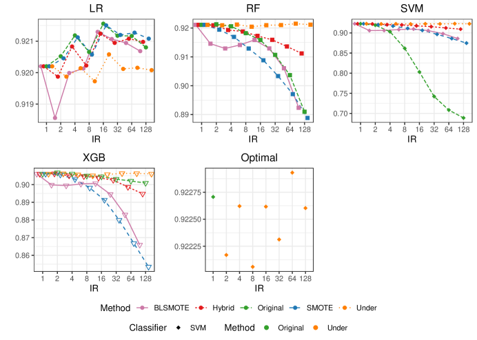
Figure 3: ROC-AUC of different methods in Example 1(a). The minimum and maximum of standard error: LR(0.0003, 0.0005), RF(0.0004,0.0007), SVM(0.0003,0.0029), XGB(0.0005, 0.0013).

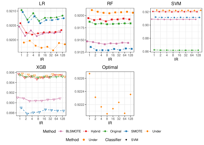
Figure 4: ROC-AUC of different methods in Example 1(b). The minimum and maximum of standard error: LR(0.0003, 0.0005), RF(0.0003,0.0006), SVM(0.0003,0.0010), XGB(0.0005, 0.0008).

5.3.1 Classical classification paradigm.

We first focus on analyzing the results for Example 1. Figures 5 and 6 exhibit the risk of different methods. We observe that the empirical risk of all classifiers without resampling is smaller than that with any resampling technique in most cases, and decreases as IR increases. This is in line with our intuition that if the risk is the primary measure of interest, we would be better off not applying any resampling techniques. In addition, we observe that only undersampling leads to a stable risk when the IR increases for all four base classification methods considered. Finally, the resampling techniques can make risk more stable across all IRs in Figure 6.

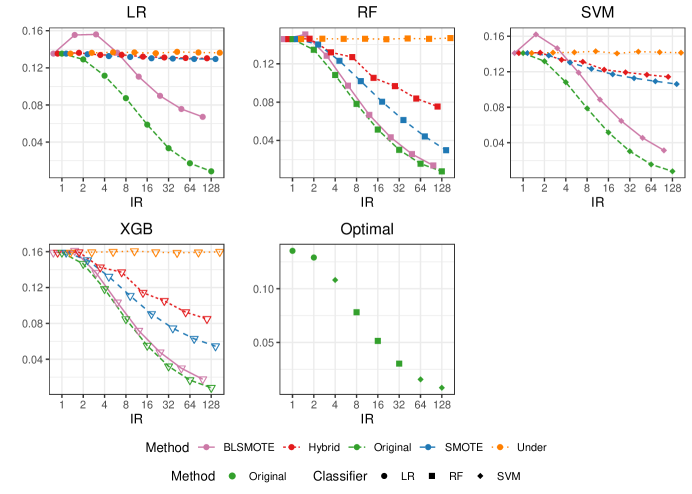
Figure 5: Risk of different methods under CC paradigm in Example 1(a). The minimum and maximum of standard error: LR(0, 0.0011), RF(0,0.0014), SVM(0,0.0012), XGB(0, 0.0014).

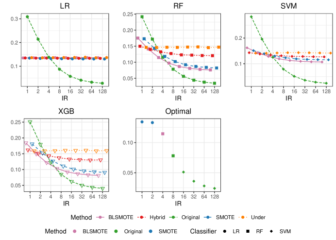
Figure 6: Risk of different methods under CC paradigm in Example 1(b). The minimum and maximum of standard error: LR(0.0001, 0.0018), RF(0.0002,0.0016), SVM(0.0001,0.0016), XGB(0.0002, 0.0016).

As mentioned in Section 2, minimizing the risk with imbalanced data could lead to large type I errors, demonstrated clearly in Figure 7. By using the resampling techniques, however, we can have much better control over type I error as IR increases. In particular, undersampling works well for all four classification methods. Lastly, we note that the optimal choices when IR $>1$ all involve resampling techniques.

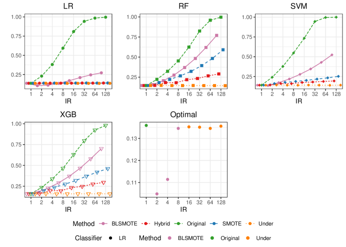
Figure 7: Type I error of different methods under CC paradigm in Example 1(a). The minimum and maximum of standard error: LR(0, 0.0037), RF(0,0.0032), SVM(0,0.0034), XGB(0, 0.0027).

The figures for Example 2 convey a similar message as in Example 1 that we do not need any resampling if the goal is to minimize the risk. On the other hand, applying certain resampling techniques is critical to bring down the type I error and increase the ROC-AUC value. Again, we omit these figures to save space.

5.3.2 Cost-Sensitive learning paradigm.

When we are in the CS learning paradigm, the objective is to minimize the expected total misclassification cost. We again first look at the results from Example 1. Naturally, we would like to see the impact of the resampling techniques on different classification methods in terms of empirical cost, which is summarized in Figures 8 and 9. From the figures, we observe that no resampling leads to the smallest cost in most cases. When IR is large, BLSMOTE leads to the smallest cost for SVM.

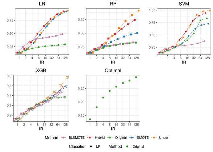
Figure 8: Cost of different methods under CS learning paradigm in Example 1(a). The minimum and maximum of standard error: LR(0.0006, 0.0066), RF(0.0007,0.0068), SVM(0.0004,0.0113), XGB(0.0004, 0.0066).

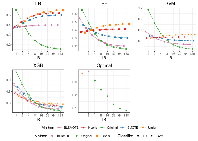
Figure 9: Cost of different methods under CS learning paradigm in Example 1(b). The minimum and maximum of standard error: LR(0.0006, 0.0061), RF(0.0008,0.0054), SVM(0.0003,0.0075), XGB(0.0005, 0.0065).

Now, we look at the results for type I error in Figures 10 and 11, where we discover that all classification methods benefit significantly from resampling techniques with undersampling being the best choice for most scenarios.

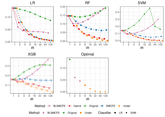
Figure 10: Type I error of different methods under CS learning paradigm in Example 1(a). The minimum and maximum of standard error: LR(0.0002, 0.0014), RF(0.0002,0.0017), SVM(0,0.0078), XGB(0.0007, 0.0019).

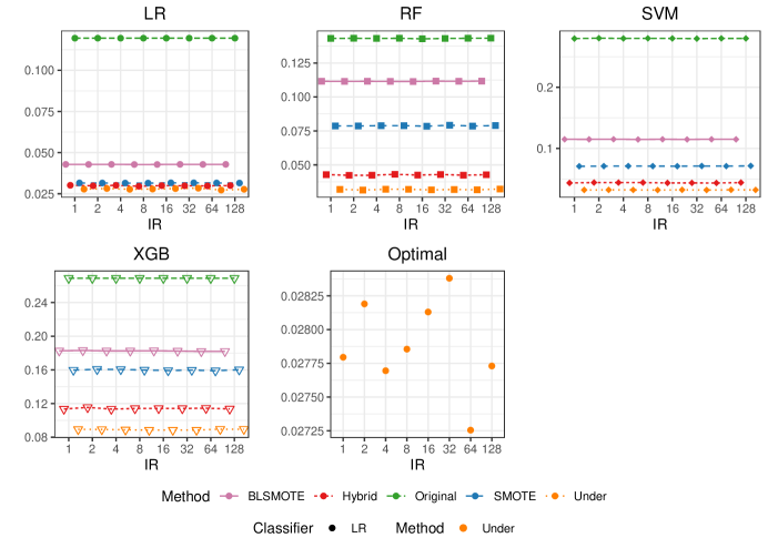
Figure 11: Type I error of different methods under CS learning paradigm in Example 1(b). The minimum and maximum of standard error: LR(0.0006, 0.0010), RF(0.0006,0.0015), SVM(0.0008,0.0019), XGB(0.0010, 0.0017).

5.3.3 Neyman-Pearson paradigm.

The NP paradigm aims to minimize type II error while controlling type I error under a target level $\alpha$. In the current implementation, we set $\alpha=0.05$. From Figures 12 and 13, we observe that the type I errors are well-controlled under $\alpha$ throughout all IRs for all base classification methods in Examples 1(a) and 1(b).

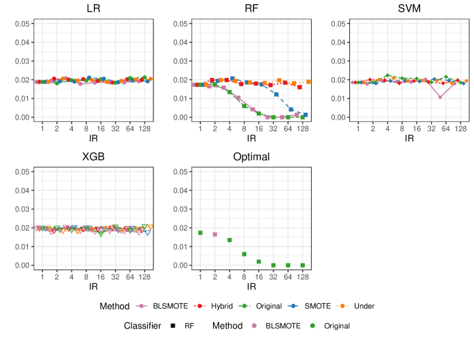
Figure 12: Type I error of different methods under NP paradigm in Example 1(a). The minimum and maximum of standard error: LR(0.0010, 0.0014), RF(0,0.0015), SVM(0.0009,0.0015), XGB(0.0009, 0.0013).

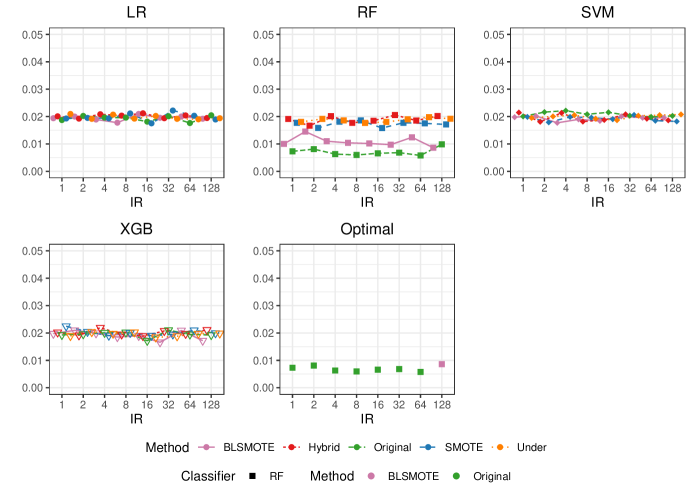
Figure 13: Type I error of different methods under NP paradigm in Example 1(b). The minimum and maximum of standard error: LR(0.0009, 0.0014), RF(0.0010,0.0017), SVM(0.0009,0.0015), XGB(0.0009, 0.0014).

When we look at Figure 14, the benefits that resampling techniques can bring are apparent in most cases. Undersampling or hybrid resampling leads to a type II error well under control. Moreover, Type II error is more robust when different IRs are selected for the test data set.

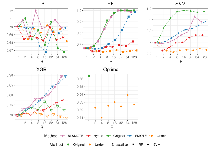
Figure 14: Type II error of different methods under NP paradigm in Example 1(a). The minimum and maximum of standard error: LR(0.0142, 0.0182), RF(0,0.0219), SVM(0.0015,0.0149), XGB(0.0081, 0.0140).

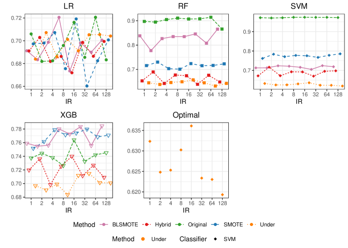
Figure 15: Type II error of different methods under NP paradigm in Example 1(b). The minimum and maximum of standard error: LR(0.0137, 0.0174), RF(0.0126,0.0232), SVM(0.0023,0.0153), XGB(0.0097, 0.0136).

For Example 2, we have the same conclusion that resampling techniques can help to reduce type II error with the type I error well-controlled under $\alpha$.

5.3.4 Summary.

In addition to the plots, we summarize in Tables 4, 5, 6, 7 the winning frequency of resampling techniques and classification methods in terms of each evaluation metric of all IRs in Examples 1(a), 1(b), 2(a), and 2(b), respectively. The number in each cell of tables represents the winning frequency for each base classification method or each resampling technique for the given metric. The numbers in bold represent the most frequent winning combination of resampling techniques and classification methods. Clearly, the optimal choices differ for different evaluation metrics, IRs, and data generation mechanisms. From these tables and the above figures, we can draw the following conclusions:

1. All the classifiers can control the type I error under a certain level $\alpha$ under the NP paradigm (see Figures 12 and 13).

2. For most base classification methods, ROC-AUC can usually benefit from resampling techniques, whether or not the test class proportion is at the same level of imbalance as the training set (see Figures 3 and 4).

3. Resampling techniques, in general, bring down the type I error regardless of the classification paradigm (see Figures 7 and 11).

4. The optimal combination of base classification method and resampling technique should be interpreted together with both the paradigm and evaluation metric. For example, in Table 4, the combination “LR+Under” leads to the minimal type I error under the CC paradigm.

5. When the training class proportion is fixed and IR varies for the test data set, the results are robust in most cases (see Figures 6, 11, and 15).

Table 4: The frequency of winning methods in Example 1(a).

	LR	RF	SVM	XGB	BLSMOTE	Hybrid	Original	SMOTE	Under
AUC	0	0	8	0	0	0	1	0	7
PR-AUC(0)	0	5	3	0	1	0	6	0	1
PR-AUC(1)	0	0	8	0	0	0	1	0	7
CC-Type I	8	0	0	0	3	0	1	0	4
CS-Type I	4	0	4	0	2	0	1	0	5
NP-Type I	0	8	0	0	1	0	7	0	0
Type I	12	8	4	0	6	0	9	0	9
CC-Type II	1	0	7	0	0	0	8	0	0
CS-Type II	1	0	4	3	1	0	7	0	0
NP-Type II	0	1	7	0	0	0	1	0	7
Type II	2	1	18	3	1	0	16	0	7
CS-Cost	8	0	0	0	0	0	8	0	0
CC-Risk	2	3	3	0	0	0	8	0	0
NP-Risk	0	1	7	0	0	0	1	0	7
Risk	2	4	10	0	0	0	9	0	7
CC-$F$-score(0)	3	4	0	1	5	0	1	2	0
CS-$F$-score(0)	2	0	4	2	1	0	7	0	0
NP-$F$-score(0)	0	2	6	0	0	0	1	0	7
$F$-score(0)	5	6	10	3	6	0	9	2	7
CC-$F$-score(1)	2	1	5	0	0	0	8	0	0
CS-$F$-score(1)	1	0	4	3	1	0	7	0	0
NP-$F$-score(1)	0	1	7	0	0	0	1	0	7
$F$-score(1)	3	2	16	3	1	0	16	0	7
Total	32	26	77	9	15	0	75	2	52

Table 5: The frequency of winning methods in Example 1(b).

	LR	RF	SVM	XGB	BLSMOTE	Hybrid	Original	SMOTE	Under
AUC	0	0	8	0	0	0	0	0	8
PR-AUC(0)	0	5	3	0	0	0	8	0	0
PR-AUC(1)	0	0	8	0	0	0	0	0	8
CC-Type I	8	0	0	0	7	0	0	0	1
CS-Type I	8	0	0	0	0	0	0	0	8
NP-Type I	0	8	0	0	1	0	7	0	0
Type I	16	8	0	0	8	0	7	0	9
CC-Type II	2	2	4	0	1	0	5	2	0
CS-Type II	0	0	8	0	0	0	8	0	0
NP-Type II	0	0	8	0	0	0	0	0	8
Type II	2	2	20	0	1	0	13	2	8
CS-Cost	3	0	5	0	1	0	6	0	1
CC-Risk	2	2	4	0	1	0	5	2	0
NP-Risk	0	0	8	0	0	0	0	0	8
Risk	2	2	12	0	1	0	5	2	8
CC-$F$-score(0)	3	2	3	0	2	0	4	2	0
CS-$F$-score(0)	2	0	6	0	0	0	8	0	0
NP-$F$-score(0)	0	0	8	0	0	0	0	0	8
$F$-score(0)	5	2	17	0	2	0	12	2	8
CC-$F$-score(1)	1	2	5	0	1	0	6	1	0
CS-$F$-score(1)	1	0	7	0	0	0	8	0	0
NP-$F$-score(1)	0	0	8	0	0	0	0	0	8
$F$-score(1)	2	2	20	0	1	0	14	1	8
Total	30	21	93	0	14	0	65	7	58

Table 6: The frequency of winning methods in Example 2(a).

	LR	RF	SVM	XGB	BLSMOTE	Hybrid	Original	SMOTE	Under
AUC	0	0	8	0	0	0	1	0	7
PR-AUC(0)	0	0	8	0	0	0	1	0	7
PR-AUC(1)	0	0	8	0	0	0	1	0	7
CC-Type I	0	0	8	0	0	0	1	0	7
CS-Type I	6.1	0	1.9	0	0.9	1.4	1	2.4	2.3
NP-Type I	3	5	0	0	2	0	5	0	1
Type I	9.1	5	9.9	0	2.9	1.4	7	2.4	10.3
CC-Type II	7	0	1	0	0	0	8	0	0
CS-Type II	0	0	3	5	1	0	7	0	0
NP-Type II	0	5	3	0	0	2	1	0	5
Type II	7	5	7	5	1	2	16	0	5
CS-Cost	0	3	4	1	6	0	1	1	0
CC-Risk	7	0	1	0	0	0	8	0	0
NP-Risk	0	4	4	0	0	2	1	0	5
Risk	7	4	5	0	0	2	9	0	5
CC-$F$-score(0)	0	0	8	0	0	0	1	0	7
CS-$F$-score(0)	0	0	7	1	5	0	1	1	1
NP-$F$-score(0)	0	5	3	0	0	2	1	0	5
$F$-score(0)	0	5	18	1	5	2	3	1	13
CC-$F$-score(1)	7	0	1	0	0	0	8	0	0
CS-$F$-score(1)	0	0	3	5	1	0	7	0	0
NP-$F$-score(1)	0	5	3	0	0	2	1	0	5
$F$-score(1)	7	5	7	5	1	2	16	0	5
Total	30.1	27	74.9	12	15.9	9.4	55	4.4	59.3

Table 7: The frequency of winning methods in Example 2(b).

	LR	RF	SVM	XGB	BLSMOTE	Hybrid	Original	SMOTE	Under
AUC	0	0	8	0	0	0	0	0	8
PR-AUC(0)	0	0	8	0	0	0	0	0	8
PR-AUC(1)	0	0	8	0	0	0	0	0	8
CC-Type I	0	0	8	0	0	0	0	0	8
CS-Type I	8	0	0	0	2	2	0	2	2
NP-Type I	0	8	0	0	2	0	6	0	0
Type I	8	8	8	0	4	2	6	2	10
CC-Type II	8	0	0	0	0	0	8	0	0
CS-Type II	0	0	0	8	0	0	8	0	0
NP-Type II	0	6	2	0	0	3	0	0	5
Type II	8	6	2	8	0	3	16	0	5
CS-Cost	1	1	2	4	1	0	4	1	2
CC-Risk	7	0	1	0	0	0	7	0	1
NP-Risk	0	6	2	0	0	4	0	0	4
Risk	7	6	3	0	0	4	7	0	5
CC-$F$-score(0)	0	0	8	0	3	1	0	0	4
CS-$F$-score(0)	0	1	4	3	4	0	3	1	0
NP-$F$-score(0)	0	6	2	0	0	4	0	0	4
$F$-score(0)	0	7	14	3	7	5	3	1	8
CC-$F$-score(1)	8	0	0	0	0	0	8	0	0
CS-$F$-score(1)	0	0	0	8	0	0	8	0	0
NP-$F$-score(1)	0	6	2	0	0	3	0	0	5
$F$-score(1)	8	6	2	8	0	3	16	0	5
Total	32	34	55	23	12	17	52	4	59

6 Real Data-Credit Card Fraud Detection

The Credit Card Transaction Data is available at http://kaggle.com/mlg-ulb/creditcardfraud. It includes credit card transactions made in September 2013 by European cardholders. In particular, it contains transactions that occurred in two days, where we have 492 frauds out of 284,807 transactions. Therefore, this data set is highly imbalanced with an imbalance ratio (IR) about 578 (284,315/492). Due to confidentiality issues, the website does not provide the original features and more background information about this data set. Features V1, V2, $\ldots$, V28 are the principal components obtained with PCA. The only features which have not been transformed with PCA are “Time” and “Amount”. Feature “Time” contains the seconds elapsed between each transaction and the first transaction in the data set. The feature “Amount” is the transaction amount. They are scaled to zero mean and unit variance. Using the feature “Class”, we redefine “0” as the fraud class (class 0) and “1” as the no-fraud class (class 1). We use the features V1, V2, $\ldots$, V28, Time and Amount as predictor variables for the classification methods.

We specify the imbalance ratio (IR) as 128 for training data set and extract a subsample from this large dataset. In particular, we randomly sample $n_{0}=300$ data points from class 0 (fraud) and $n1=n0*\mbox{IR}=38,400$ from class 1 (no-fraud). This procedure creates our training data set. The test data set contains a random sample of $m_{0}=192$ for class 0 and $m_{1}=m_{0}*\mbox{IR}_{test}$ for class 1 from the remaining data, where $\mbox{IR}_{test}$ varies in $\{2^{i},i=0,1,\cdots,7\}$. This splitting mechanism implies that IR will be different for the training and test data sets.

The remaining implementation details are the same as in Section 5.2. We still repeat the experiment 100 times and report the average performance and frequency of winning methods by the mean for each metric and classification paradigm combination. The frequency of winning methods were summarized in Table 8 and report Figures 16 and 17 and omit the other figures since they convey similar information to that in Section 5.3.

From Figures 16 and 17, resampling techniques are in general beneficial for the metrics in most cases. In addition, most of the results are robust when the test IR increases. This is consistent with the simulation results. Table 8 shows that the combination “RF+Hybrid” has the top performance. Note that this appears to be different from the choices implied by Tables 4-7, which again show that the best performing method highly depends on the data generation process. This actually agrees with our understanding of SVM vs. RF in that RF may be more effective than SVM in a more complex scenario. Moreover, the optimal methods depend on the learning paradigm and evaluation metrics. For example, if our objective is to minimize the overall risk under the CC paradigm, “RF+SMOTE” is the best choice in Table 8; if our objective is to minimize the type II error while controlling the type I error under a specific level, “RF+Hybrid” performs the best. Therefore, there is no universal best combination for the imbalanced classification problem.

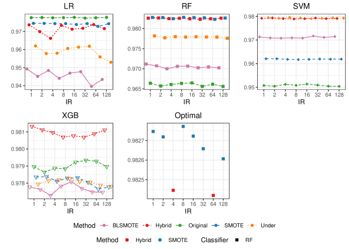
Figure 16: ROC-AUC of different methods in real data. The minimum and maximum of standard error: LR(0.0005, 0.0089), RF(0.0005,0.0009), SVM(0.0005,0.0014), XGB(0.0005, 0.0007).

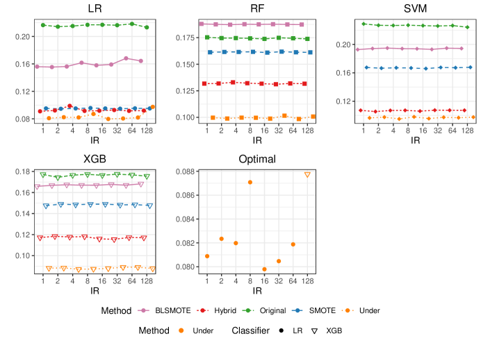
Figure 17: Type I error of different methods under CC paradigm in real data. The minimum and maximum of standard error: LR(0.0020, 0.0086), RF(0.0019,0.0024), SVM(0.0019,0.0036), XGB(0.0018, 0.0023).

Table 8: The frequency of winning methods when IR of test data varies in credit fraud detection.

	LR	RF	SVM	XGB	BLSMOTE	Hybrid	Original	SMOTE	Under
AUC	0	8	0	0	0	2	0	6	0
PR-AUC(0)	0	8	0	0	0	0	0	8	0
PR-AUC(1)	0	8	0	0	0	8	0	0	0
CC-Type I	7	0	0	1	0	0	0	0	8
CS-Type I	0	0	8	0	0	0	0	0	8
NP-Type I	0	8	0	0	0	0	8	0	0
Type I	7	8	8	1	0	0	8	0	16
CC-Type II	0	0	4	4	0	0	8	0	0
CS-Type II	0	0	0	8	0	0	8	0	0
NP-Type II	0	6	2	0	0	6	0	0	2
Type II	0	6	6	12	0	6	16	0	2
CS-Cost	0	1	0	7	0	2	3	3	0
CC-Risk	1	3	0	4	0	3	1	4	0
NP-Risk	0	6	2	0	0	6	0	0	2
Risk	1	9	2	4	0	9	1	4	2
CC-$F$-score(0)	1	3	0	4	0	4	1	3	0
CS-$F$-score(0)	0	0	0	8	0	0	6	2	0
NP-$F$-score(0)	0	8	0	0	0	8	0	0	0
$F$-score(0)	1	11	0	12	0	12	7	5	0
CC-$F$-score(1)	1	4	0	3	0	3	1	4	0
CS-$F$-score(1)	0	0	0	8	0	0	6	2	0
NP-$F$-score(1)	0	6	2	0	0	6	0	0	2
$F$-score(1)	1	10	2	11	0	9	7	6	2
Total	10	69	18	47	0	48	42	32	22

7 Discussion

In this paper, we review the imbalanced classification with a paradigm-based view. In addition to the few take-away messages we offered in the simulation section, the main message from the review is that there is no single best approach to imbalanced classification. The optimal choice for resampling techniques and base classification methods highly depends on the classification paradigms, evaluation metric, as well as the severity of imbalancedness (imbalance ratio).

Admittedly, we only considered a selective list of resampling techniques and base classification methods. There are many other combinations that are worth further consideration. In addition, we presented results from two simulated data generation processes as well as a real data set, which could be unrepresentative for specific applications. We suggest practitioners adapt our analysis process for evaluating different choices for imbalanced classification to align with their data generation mechanism.

Furthermore, in our numerical experiments, all base classification methods were applied using the corresponding R-packages with their default parameters. Note that although we didn’t tune the parameters due to the already-extensive simulation settings, it is well known that parameter tuning could further improve the performance of a classifier in certain situation. For example, the parameter $k$ in SMOTE Chawla et al. (2002) can be selected via cross-validation. We leave a systematic study of the impact of parameter tuning on imbalanced classification as a future research topic.

Lastly, we focused on binary classification throughout the review. We expect similar interpretations and conclusions from multi-class imbalanced classification.

References

- Alahmari [2020] Fahad Alahmari. A comparison of resampling techniques for medical data using machine learning. Journal of Information & Knowledge Management, 19(01):2040016, 2020.
- Altman [1992] Naomi S Altman. An introduction to kernel and nearest-neighbor nonparametric regression. The American Statistician, 46(3):175–185, 1992.
- Anis et al. [2020] Maira Anis, Mohsin Ali, Shahid Aslam Mirza, and Malik Mamoon Munir. Analysis of resampling techniques on predictive performance of credit card classification. Modern Applied Science, 14(7), 2020.
- Arnqvist et al. [2021] Natalya Pya Arnqvist, Blaise Ngendangenzwa, Eric Lindahl, Leif Nilsson, and Jun Yu. Efficient surface finish defect detection using reduced rank spline smoothers and probabilistic classifiers. Econometrics and Statistics, 18:89–105, 2021.
- Beaulieu et al. [2014] Chandree L Beaulieu, Jacek Majewski, Jeremy Schwartzentruber, Mark E Samuels, Bridget A Fernandez, Francois P Bernier, Michael Brudno, Bartha Knoppers, Janet Marcadier, David Dyment, et al. Forge canada consortium: outcomes of a 2-year national rare-disease gene-discovery project. The American Journal of Human Genetics, 94(6):809–817, 2014.
- Bradford et al. [1998] Jeffrey P Bradford, Clayton Kunz, Ron Kohavi, Cliff Brunk, and Carla E Brodley. Pruning decision trees with misclassification costs. In European Conference on Machine Learning, pages 131–136. Springer, 1998.
- Bradley [1997] Andrew P Bradley. The use of the area under the roc curve in the evaluation of machine learning algorithms. Pattern recognition, 30(7):1145–1159, 1997.
- Breiman [2001] Leo Breiman. Random forests. Machine learning, 45(1):5–32, 2001.
- Cannon et al. [2002] Adam Cannon, James Howse, Don Hush, and Clint Scovel. Learning with the neyman-pearson and min-max criteria. Los Alamos National Laboratory, Tech. Rep. LA-UR, pages 02–2951, 2002.
- Cao et al. [2014] Peng Cao, Jinzhu Yang, Wei Li, Dazhe Zhao, and Osmar Zaiane. Ensemble-based hybrid probabilistic sampling for imbalanced data learning in lung nodule cad. Computerized Medical Imaging and Graphics, 38(3):137–150, 2014.
- Castro and Braga [2013] Cristiano L Castro and Antônio P Braga. Novel cost-sensitive approach to improve the multilayer perceptron performance on imbalanced data. IEEE transactions on neural networks and learning systems, 24(6):888–899, 2013.
- Cateni et al. [2014] Silvia Cateni, Valentina Colla, and Marco Vannucci. A method for resampling imbalanced datasets in binary classification tasks for real-world problems. Neurocomputing, 135:32–41, 2014.
- Chawla et al. [2002] Nitesh V Chawla, Kevin W Bowyer, Lawrence O Hall, and W Philip Kegelmeyer. Smote: synthetic minority over-sampling technique. Journal of artificial intelligence research, 16:321–357, 2002.
- Chen and Guestrin [2016] Tianqi Chen and Carlos Guestrin. Xgboost: A scalable tree boosting system. In Proceedings of the 22nd acm sigkdd international conference on knowledge discovery and data mining, pages 785–794. ACM, 2016.
- Chen et al. [2019] Tianqi Chen, Tong He, Michael Benesty, Vadim Khotilovich, Yuan Tang, Hyunsu Cho, Kailong Chen, Rory Mitchell, Ignacio Cano, Tianyi Zhou, Mu Li, Junyuan Xie, Min Lin, Yifeng Geng, and Yutian Li. xgboost: Extreme Gradient Boosting, 2019. URL https://CRAN.R-project.org/package=xgboost. R package version 0.90.0.2.
- Chen [2016] You-Shyang Chen. An empirical study of a hybrid imbalanced-class dt-rst classification procedure to elucidate therapeutic effects in uremia patients. Medical & biological engineering & computing, 54(6):983–1001, 2016.
- Cortes and Vapnik [1995] Corinna Cortes and Vladimir Vapnik. Support-vector networks. Machine learning, 20(3):273–297, 1995.
- Davis and Goadrich [2006] Jesse Davis and Mark Goadrich. The relationship between precision-recall and roc curves. In Proceedings of the 23rd international conference on Machine learning, pages 233–240. ACM, 2006.
- Díez-Pastor et al. [2015] José F Díez-Pastor, Juan J Rodríguez, César García-Osorio, and Ludmila I Kuncheva. Random balance: ensembles of variable priors classifiers for imbalanced data. Knowledge-Based Systems, 85:96–111, 2015.
- Domingos [1999] Pedro Domingos. Metacost: A general method for making classifiers cost-sensitive. In KDD, volume 99, pages 155–164, 1999.
- Elkan [2001] Charles Elkan. The foundations of cost-sensitive learning. In International joint conference on artificial intelligence, volume 17, pages 973–978. Lawrence Erlbaum Associates Ltd, 2001.
- García et al. [2012a] Vicente García, José Salvador Sánchez, Raúl Martín-Félez, and Ramón Alberto Mollineda. Surrounding neighborhood-based smote for learning from imbalanced data sets. Progress in Artificial Intelligence, 1(4):347–362, 2012a.
- García et al. [2012b] Vicente García, José Salvador Sánchez, and Ramón Alberto Mollineda. On the effectiveness of preprocessing methods when dealing with different levels of class imbalance. Knowledge-Based Systems, 25(1):13–21, 2012b.
- Goadrich et al. [2004] Mark Goadrich, Louis Oliphant, and Jude Shavlik. Learning ensembles of first-order clauses for recall-precision curves: A case study in biomedical information extraction. In International Conference on Inductive Logic Programming, pages 98–115. Springer, 2004.
- Guo et al. [2017] Haixiang Guo, Yijing Li, Jennifer Shang, Mingyun Gu, Yuanyue Huang, and Bing Gong. Learning from class-imbalanced data: Review of methods and applications. Expert Systems with Applications, 73:220–239, 2017.
- Han et al. [2005] Hui Han, Wen-Yuan Wang, and Bing-Huan Mao. Borderline-smote: a new over-sampling method in imbalanced data sets learning. In International conference on intelligent computing, pages 878–887. Springer, 2005.
- Hastie et al. [2009] Trevor Hastie, Robert Tibshirani, and Jerome Friedman. The elements of statistical learning: data mining, inference, and prediction. Springer Science & Business Media, 2009.
- He et al. [2008] Haibo He, Yang Bai, Edwardo A Garcia, and Shutao Li. Adasyn: Adaptive synthetic sampling approach for imbalanced learning. In 2008 IEEE International Joint Conference on Neural Networks (IEEE World Congress on Computational Intelligence), pages 1322–1328. IEEE, 2008.
- Huang and Ling [2005] Jin Huang and Charles X Ling. Using auc and accuracy in evaluating learning algorithms. IEEE Transactions on knowledge and Data Engineering, 17(3):299–310, 2005.
- James et al. [2013] Gareth James, Daniela Witten, Trevor Hastie, and Robert Tibshirani. An introduction to statistical learning, volume 112. Springer, 2013.
- Koltchinskii [2011] Vladimir Koltchinskii. Oracle Inequalities in Empirical Risk Minimization and Sparse Recovery Problems: Ecole d’Eté de Probabilités de Saint-Flour XXXVIII-2008, volume 2033. Springer Science & Business Media, 2011.
- Kotsiantis et al. [2007] Sotiris B Kotsiantis, I Zaharakis, and P Pintelas. Supervised machine learning: A review of classification techniques. Emerging artificial intelligence applications in computer engineering, 160:3–24, 2007.
- Kubat et al. [1998] Miroslav Kubat, Robert C Holte, and Stan Matwin. Machine learning for the detection of oil spills in satellite radar images. Machine learning, 30(2):195–215, 1998.
- Kuhn and Johnson [2013] Max Kuhn and Kjell Johnson. Applied predictive modeling, volume 26. Springer, 2013.
- Kumar et al. [2014] N Santhosh Kumar, K Nageswara Rao, A Govardhan, K Sudheer Reddy, and Ali Mirza Mahmood. Undersampled k-means approach for handling imbalanced distributed data. Progress in Artificial Intelligence, 3(1):29–38, 2014.
- Liaw and Wiener [2002] Andy Liaw and Matthew Wiener. Classification and regression by randomforest. R News, 2(3):18–22, 2002. URL https://CRAN.R-project.org/doc/Rnews/.
- Lin et al. [2002] Yi Lin, Yoonkyung Lee, and Grace Wahba. Support vector machines for classification in nonstandard situations. Machine learning, 46(1):191–202, 2002.
- Ling et al. [2004] Charles X Ling, Qiang Yang, Jianning Wang, and Shichao Zhang. Decision trees with minimal costs. In Proceedings of the twenty-first international conference on Machine learning, page 69. ACM, 2004.
- López et al. [2012] Victoria López, Alberto Fernández, Jose G Moreno-Torres, and Francisco Herrera. Analysis of preprocessing vs. cost-sensitive learning for imbalanced classification. open problems on intrinsic data characteristics. Expert Systems with Applications, 39(7):6585–6608, 2012.
- López et al. [2013] Victoria López, Alberto Fernández, Salvador García, Vasile Palade, and Francisco Herrera. An insight into classification with imbalanced data: Empirical results and current trends on using data intrinsic characteristics. Information sciences, 250:113–141, 2013.
- López et al. [2015] Victoria López, Sara Del Río, José Manuel Benítez, and Francisco Herrera. Cost-sensitive linguistic fuzzy rule based classification systems under the mapreduce framework for imbalanced big data. Fuzzy Sets and Systems, 258:5–38, 2015.
- McLachlan [2004] Geoffrey J McLachlan. Discriminant analysis and statistical pattern recognition, volume 544. John Wiley & Sons, 2004.
- Meyer et al. [2019] David Meyer, Evgenia Dimitriadou, Kurt Hornik, Andreas Weingessel, and Friedrich Leisch. e1071: Misc Functions of the Department of Statistics, Probability Theory Group (Formerly: E1071), TU Wien, 2019. URL https://CRAN.R-project.org/package=e1071. R package version 1.7-2.
- Nekooeimehr and Lai-Yuen [2016] Iman Nekooeimehr and Susana K Lai-Yuen. Adaptive semi-unsupervised weighted oversampling (a-suwo) for imbalanced datasets. Expert Systems with Applications, 46:405–416, 2016.
- Nelder and Wedderburn [1972] John Ashworth Nelder and Robert WM Wedderburn. Generalized linear models. Journal of the Royal Statistical Society: Series A (General), 135(3):370–384, 1972.
- Owen [2007] Art B Owen. Infinitely imbalanced logistic regression. Journal of Machine Learning Research, 8(4), 2007.
- Qiao and Liu [2009] Xingye Qiao and Yufeng Liu. Adaptive weighted learning for unbalanced multicategory classification. Biometrics, 65(1):159–168, 2009.
- Qiao et al. [2010] Xingye Qiao, Hao Helen Zhang, Yufeng Liu, Michael J Todd, and James Stephen Marron. Weighted distance weighted discrimination and its asymptotic properties. Journal of the American Statistical Association, 105(489):401–414, 2010.
- Ranneby and Yu [2011] Bo Ranneby and Jun Yu. Nonparametric and probabilistic classification using nn-balls with environmental and remote sensing applications. In Advances in Directional and Linear Statistics, pages 201–216. Springer, 2011.
- Rigollet and Tong [2011] Philippe Rigollet and Xin Tong. Neyman-pearson classification, convexity and stochastic constraints. Journal of Machine Learning Research, 12(Oct):2831–2855, 2011.
- Rish et al. [2001] Irina Rish et al. An empirical study of the naive bayes classifier. In IJCAI 2001 workshop on empirical methods in artificial intelligence, volume 3, pages 41–46, 2001.
- Rumelhart et al. [1985] David E Rumelhart, Geoffrey E Hinton, and Ronald J Williams. Learning internal representations by error propagation. Technical report, California Univ San Diego La Jolla Inst for Cognitive Science, 1985.
- Sáez et al. [2015] José A Sáez, Julián Luengo, Jerzy Stefanowski, and Francisco Herrera. Smote–ipf: Addressing the noisy and borderline examples problem in imbalanced classification by a re-sampling method with filtering. Information Sciences, 291:184–203, 2015.
- Safavian and Landgrebe [1991] S Rasoul Safavian and David Landgrebe. A survey of decision tree classifier methodology. IEEE transactions on systems, man, and cybernetics, 21(3):660–674, 1991.
- Singla and Domingos [2005] Parag Singla and Pedro Domingos. Discriminative training of markov logic networks. In AAAI, volume 5, pages 868–873, 2005.
- Siriseriwan [2019] Wacharasak Siriseriwan. smotefamily: A Collection of Oversampling Techniques for Class Imbalance Problem Based on SMOTE, 2019. URL https://CRAN.R-project.org/package=smotefamily. R package version 1.3.1.
- Sun et al. [2007] Yanmin Sun, Mohamed S Kamel, Andrew KC Wong, and Yang Wang. Cost-sensitive boosting for classification of imbalanced data. Pattern Recognition, 40(12):3358–3378, 2007.
- Sun et al. [2009] Yanmin Sun, Andrew KC Wong, and Mohamed S Kamel. Classification of imbalanced data: A review. International Journal of Pattern Recognition and Artificial Intelligence, 23(04):687–719, 2009.
- Sun et al. [2015] Zhongbin Sun, Qinbao Song, Xiaoyan Zhu, Heli Sun, Baowen Xu, and Yuming Zhou. A novel ensemble method for classifying imbalanced data. Pattern Recognition, 48(5):1623–1637, 2015.
- Tong [2013] Xin Tong. A plug-in approach to neyman-pearson classification. The Journal of Machine Learning Research, 14(1):3011–3040, 2013.
- Tong et al. [2016] Xin Tong, Yang Feng, and Anqi Zhao. A survey on neyman-pearson classification and suggestions for future research. Wiley Interdisciplinary Reviews: Computational Statistics, 8(2):64–81, 2016.
- Tong et al. [2018] Xin Tong, Yang Feng, and Jingyi Jessica Li. Neyman-pearson classification algorithms and np receiver operating characteristics. Science advances, 4(2):eaao1659, 2018.
- Turney [1994] Peter D Turney. Cost-sensitive classification: Empirical evaluation of a hybrid genetic decision tree induction algorithm. Journal of artificial intelligence research, 2:369–409, 1994.
- Voigt et al. [2014] Tobias Voigt, Roland Fried, Michael Backes, and Wolfgang Rhode. Threshold optimization for classification in imbalanced data in a problem of gamma-ray astronomy. Advances in Data Analysis and Classification, 8(2):195–216, 2014.
- Wang and Japkowicz [2010] Benjamin X Wang and Nathalie Japkowicz. Boosting support vector machines for imbalanced data sets. Knowledge and information systems, 25(1):1–20, 2010.
- Wei et al. [2013] Wei Wei, Jinjiu Li, Longbing Cao, Yuming Ou, and Jiahang Chen. Effective detection of sophisticated online banking fraud on extremely imbalanced data. World Wide Web, 16(4):449–475, 2013.
- Yen and Lee [2009] Show-Jane Yen and Yue-Shi Lee. Cluster-based under-sampling approaches for imbalanced data distributions. Expert Systems with Applications, 36(3):5718–5727, 2009.
- Youn and McLeod [2007] Seongwook Youn and Dennis McLeod. A comparative study for email classification. In Advances and innovations in systems, computing sciences and software engineering, pages 387–391. Springer, 2007.
- Zadrozny et al. [2003] Bianca Zadrozny, John Langford, and Naoki Abe. Cost-sensitive learning by cost-proportionate example weighting. In ICDM, volume 3, page 435, 2003.
- Zhang et al. [2016] Chenggang Zhang, Wei Gao, Jiazhi Song, and Jinqing Jiang. An imbalanced data classification algorithm of improved autoencoder neural network. In 2016 Eighth International Conference on Advanced Computational Intelligence (ICACI), pages 95–99. IEEE, 2016.
- Zheng et al. [2004] Zhaohui Zheng, Xiaoyun Wu, and Rohini Srihari. Feature selection for text categorization on imbalanced data. ACM Sigkdd Explorations Newsletter, 6(1):80–89, 2004.
- Zhou and Liu [2005] Zhi-Hua Zhou and Xu-Ying Liu. Training cost-sensitive neural networks with methods addressing the class imbalance problem. IEEE Transactions on knowledge and data engineering, 18(1):63–77, 2005.
- Zou et al. [2016] Quan Zou, Sifa Xie, Ziyu Lin, Meihong Wu, and Ying Ju. Finding the best classification threshold in imbalanced classification. Big Data Research, 5:2–8, 2016.