Full electromagnetic Green’s dyadic of spherically symmetric open optical systems and elimination of static modes from the resonant-state expansion

Abstract

A general analytic form of the full $6\times 6$ dyadic Green’s function of a spherically symmetric open optical system is presented, with an explicit solution provided for a homogeneous sphere in vacuum. Different spectral representations of the Green’s function are derived using the Mittag-Leffler theorem, and their convergence to the exact solution is analyzed, allowing us to select optimal representations. Based on them, more efficient versions of the resonant-state expansion (RSE) are formulated, with a particular focus on the static mode contribution, including versions of the RSE with a complete elimination of static modes. These general versions of the RSE, applicable to non-spherical optical systems, are verified and illustrated on exactly solvable examples of a dielectric sphere in vacuum with perturbations of its size and refractive index, demonstrating the same level of convergence to the exact solution for both transverse electric and transverse magnetic polarizations.

I Introduction

The electromagnetic dyadic Green’s function (GF), introduced by Schwinger more than 70 years ago, is a tensor determining the electric and magnetic fields generated by a point-like source, such as a dipole, an oscillating charge, or a current. The GF contains a complete information about the physical system and provides access to any observable, such as electromagnetic near and far field distributions Tai71 ; Chew95 , total radiation intensity and Purcell’s factor DungPRA00 ; MuljarovPRB16Purcell , optical scattering matrix and scattering cross sections LobanovPRA18 ; WeissPRB18 .

In free space, the Green’s dyadic has a closed analytic form LevineCPAM50 , clearly demonstrating its spatial singularity. This singularity has a fundamental origin related to the vectorial nature of the electromagnetic field and corresponds to the zero-frequency, i.e. static pole of the GF in the complex frequency plane, responsible for the longitudinal components of the fields. In optical systems, this static pole singularity can be strongly modified by spatial inhomogeneities of the permittivity and permeability, which presents a significant challenge for its correct calculation. A comprehensive analysis of the dyadic GFs in electromagnetic systems, including their expansion in bounded media in terms of electric and magnetic eigenmodes of optical resonators and waveguides, was presented in Tai71 . Taking into account only the physical modes (which are solenoidal in nature), this treatment, however, was lacking completeness necessary for a correct description of the static-pole singularity. Later on, this mistake was fixed TaiIEEE73 ; CollinCJP73 by adding longitudinal modes to the eigenmode expansion of the dyadic GF CollinEM86 . Still, the static pole problem has caused long debates in the literature JohnsonRS79 ; WangIEEE82 and further attempts to express the GF only in terms of the solenoidal fields PathakIEEE83 .

A more analytical approach to the dyadic GF of an open system was developed in the spirit of the scattering Mie theory MieAP08 ; Bohren1998 , by using spherical transverse functions ${\bf M}$ and ${\bf N}$, and longitudinal functions ${\bf L}$, originally introduced by Stratton Stratton41 . This approach is based on the assumption of homogeneity of a spherically symmetric system in the radial direction. Therefore, it has become a rather standard way of treating homogeneous systems Chew95 which was intensively used e.g. for multilayered spherical systems WeiIEEE94 ; OkhmatovskiIEEE03 ; KimMOTL07 ; FallahiIEEE11 . There was even an attempt to generalize this formalism for radially inhomogeneous systems YehPR63 ; however, it is not clear what are the practical benefits of the suggested generalization.

In Stratton’s theory, the static pole of the GF of a spherically symmetric multilayered system is build up with ${\bf L}$ functions leading to rather simple analytic expressions Chew95 . However, there is also a significant implicit contribution to the static pole coming from the transverse functions ${\bf M}$ and ${\bf N}$. It is not obvious whether or not this approach treats the static pole of the GF correctly, as no reliable checks of the basis completeness have been performed, to the best of our knowledge. In fact, the analytic results available for the far field (including the Mie theory itself) do not contain any contribution of static modes Stratton41 ; Bohren1998 . It is known, however, that static modes do contribute to the near field LobanovPRA18 and can influence the response of the system to excitations placed in its vicinity.

Investigating the pole structure of the dyadic GF in the complex frequency plane is equivalent to expanding it into the eigenmodes of the optical system. Until recently, such expansions were available only for bounded media, using e.g. Dirichlet boundary conditions Tai71 ; DanieleIEEE84 . For example, the correct GF of a closed spherical cavity and its expansion into the eigenmodes, with a proper account of its static pole in terms of the longitudinal modes, was presented in CollinEM86 . At the same time, similar expansions of the dyadic GFs for open systems were not available in electrodynamics. In non-relativistic quantum mechanics dealing with scalar GFs, such expansions are known as Mittag-Leffler (ML) representations MorePRA71 ; MorePRA73 . The major obstacle for applying the same principle to electrodynamics was the normalization of the electromagnetic modes of an open system which was not known. As a result, even for a homogeneous dielectric sphere in vacuum, a proper ML representation of the GF is still missing in the literature.

The electromagnetic modes of an open optical system, called resonant states (RSs) are discrete solutions of Maxwell’s equations with outgoing boundary conditions. The RS frequencies are generally complex, reflecting the fact that the energy leaks out of the system. In particular, the quality factor of a RS is given by half of the ratio of real to imaginary part of its eigenfrequency. The concept of RSs has recently become a powerful tool widely used in the literature for studying the spectral properties of open optical systems and for describing resonances observed in the optical spectra in a mathematically rigorous way MuljarovEPL10 ; DoostPRA13 ; SauvanPRL13 ; BaiOE13 ; DoostPRA14 ; MuljarovPRB16Purcell ; PerrinOE16 ; MuljarovPRB16 ; WeissPRL16 ; WeissPRB17 ; LobanovPRA17 ; LobanovPRA18 ; WeissPRB18 ; MuljarovOL18 ; BurgerPRA18 ; YanPRB18 ; Lalanne18 ; LalanneJOSAA19 ; SehmiPRB20 ; Sam19 .

Finite quality factors of the RSs, while reflecting a leakage of the electromagnetic energy contained within the system to the exterior, also lead to a catastrophic spatial divergence of the RS wave functions. As a result, the standard normalization, given by the volume integral of the square modulus of the wave function, is no longer applicable. Only recently, the correct normalization of the electromagnetic RSs has been found MuljarovEPL10 providing a general analytic expression for an arbitrary dielectric system, which was later on generalized to systems with frequency dispersion MuljarovPRB16 ; MuljarovPRB16Purcell and arbitrary permeability and chirality MuljarovOL18 .

On the other hand, in a purely numerical approach to the RS normalization developed in SauvanPRL13 , the exponential growths of the RS fields is damped by introducing so-called perfectly matched layers, artificially absorbing the diverging electromagnetic field and in this way approximating the actual open physical system with an effective closed one. This approach is using a phenomenological expansion of the dyadic GF into a few dominant eigenmodes of the effective closed system. Later on, the method was refined YanPRB18 by taking into account in the GF expansion more eigenmodes, including a large number of non-physical states of the absorbing layer, which were required for completeness. Alternative numerical approaches to the normalization and spectral representation of the GF have been also suggested BaiOE13 ; PerrinOE16 ; BurgerPRA18 . In particular, a Riesz-projection method, developed in BurgerPRA18 for an efficient treatment of optical systems in terms of only a few RSs close to the frequency range of interest, does not require any explicit mode normalization. It introduces a finite closed contour in the complex frequency plane, and numerically evaluates the contour integral, which can be understood as a modified ML representation for a limited number of RSs. A more detailed literature review of modern theoretical and computational methods based on the use of the RSs can be found e.g. in Lalanne18 ; LalanneJOSAA19 ; SehmiPRB20 .

Following the analytical approach to scalar GFs developed in quantum mechanics MorePRA71 ; MorePRA73 and using some general properties of GFs in one dimension Morse53 , a rigorous ML representation of the electromagnetic GF of a homogeneous dielectric sphere in vacuum was presented in MuljarovEPL10 for transverse electric polarization, also verifying the general analytic normalization of the RSs introduced in that work. Strictly speaking, the ML representation defines the RS normalization via the residues at the poles of the GF, which are located in the complex frequency plane exactly at the RS eigen frequencies. This allowed us to work our later on a rigorous proof of the general analytic normalization of the RSs of an arbitrary three-dimensional (3D) open optical system DoostPRA14 and to develop its further generalization MuljarovPRB16 ; MuljarovPRB16Purcell ; MuljarovOL18 and application to various geometries DoostPRA13 ; WeissPRL16 ; WeissPRB17 ; LobanovPRA17 ; Sam19 . As a result, a ML representation of the dyadic GF of an arbitrary optical system was obtained MuljarovOL18 . This form contains a summation over all the RSs of the system, supplemented with a proper set of static modes required for completeness LobanovPRA19 .

The benefit of using the ML representation of the GF is not only that it reveals the pole structure of the Green’s dyadic. It also provides the fastest calculation of the optical spectra, as it addresses all the driving frequencies simultaneously. In fact, the optical spectra are given in the form of a superposition of complex Lorentzian lines, each line due to an individual RS. Examples available in the literature include but are not limited to the exact theory of the Purcell effect MuljarovPRB16Purcell , scattering cross-section of micro- and nano-particles LobanovPRA18 , and scattering matrix of planar optical systems WeissPRB18 ; WeissPRL16 ; WeissPRB17 .

The ML representation of the GF is also at the heart of the resonant-state expansion (RSE), a novel rigorous method developed in MuljarovEPL10 for calculating the RSs of an arbitrary open optical system. The RSE maps the set of Maxwell’s equations onto a linear matrix eigenvalue problem, using the RSs of another system as a basis for expansion. The basis system differs from the target system by a perturbation and is usually (but not necessarily WeissPRL16 ; WeissPRB17 ) solvable analytically. In three dimensions, a homogeneous sphere in vacuum is obviously the simplest basis system allowing an exact analytic solution. It is important to note that the RSE is not limited to small perturbations but is capable of treating perturbations of arbitrary strength, and can be superior to existing computational methods in electrodynamics, such as finite difference in time domain and finite element methods, in terms of accuracy and efficiency, as demonstrated in DoostPRA14 ; LobanovPRA17 ; LobanovPRA19 . Another significant advantage of the RSE compared to other methods is that it calculates an asymptotically complete set of the RSs of the target system within a wide spectral range; no RSs are missing and no spurious solutions are produced. The technical implementation is also very straightforward, as the RSs of the target system are found by just diagonalizing a complex matrix containing the matrix elements of the perturbation. Finally, the RSE is a numerically exact method: The only parameter of the RSE is the size of the truncated basis which can be made arbitrarily large.

While applying the RSE to 3D open optical systems, it turned out that in addition to the RSs of the basis system, one has to include in the basis for completeness also an additional sets of static modes, in this way representing the static pole of the GF discussed above. In spite of the fact that the problem of static modes in the RSE has been addressed in DoostPRA14 ; LobanovPRA19 , the RSE method still has an unsolved fundamental problem of correct and efficient inclusion of static modes, or even their partial or complete elimination. Indeed, there is presently available either a quick but incomplete static mode inclusion DoostPRA14 , or a complete inclusion of static modes which however suffers from a too slow convergence to the exact solution LobanovPRA19 .

The purpose of the present paper is two-fold: (i) to derive explicit analytic expressions for the dyadic GF of a spherically symmetric system and to find its ML representations properly describing the static pole of the GF, and (ii) to address the static-mode challenge of the RSE, by developing new exact and quickly convergent versions of the method.

As for the first aim, the general analytic form of the full dyadic GF of an arbitrary spherically symmetric system, which we derive in this paper, has not been presented in the literature, to the best of our knowledge. In particular, the provided solution has a number of important features which have not been addressed.

First of all, instead of using the widely applied Stratton’s functions ${\bf M}$, ${\bf N}$, and ${\bf L}$, having a specific radial dependence, we implement the formalism of vector spherical harmonics (VSHs) BarreraEJP85 . These do not depend on the radial coordinate and are thus suited for treating any radial inhomogeneity. The basis of VSHs provides an elegant mapping of Maxwell’s equations onto a 1st-order matrix differential equation describing the radial dependence of the fields. This formalism is useful also for non-spherical systems, as in the far field any solution naturally splits into spherical waves described by the VSHs. Importantly, the latter present a useful basis for calculating the light scattering LobanovPRA18 ; WeissPRB18 .

Secondly, the electromagnetic Green’s dyadic is defined in the literature as either electric or, rarely, magnetic Green’s tensor of Maxwell’s wave equation for, respectively, the electric or magnetic field. Only recently, the full electromagnetic dyadic GF for the set of Maxwell’s equations was introduced in MuljarovOL18 , with both electric and magnetic components contributing on equal footing. Following MuljarovOL18 , we treat here the full $6\times 6$ Green’s tensor satisfying the first-order Maxwell equations with point-like source terms.

Thirdly, for spherically symmetric systems, we obtain a general analytic form of the full dyadic GF, after splitting it into two orthogonal polarizations, transverse electric (TE) and transverse magnetic (TM). Furthermore, we analyze the pole structure of the dyadic GF in the complex frequency plane and derive ML representations properly treating the static pole. Finally, we derive explicit analytic expressions for the GF of a homogeneous sphere in vacuum, even though this solution is available in the literature in some form Chew95 ; KaliteevskiPRB01 ; ChoPRB02 ; GlazovPSS11 . We emphasize, however, that a valid ML representation of the GF of a sphere and in particular a correct treatment of its static pole is still missing. Since the RSE is normally using a homogeneous sphere as a basis system, it is very important to know the correct analytic form and a proper ML representation of its dyadic GF.

The correct treatment of the static pole of the dyadic GF is one of the main achievements of the present work. Based on this knowledge, the full ML expansion of the GF is presented in several different ways. Different ML representations can also lead to different versions of the RSE. This flexibility is due to the energetic degeneracy of static modes, so that one can use any suited basis in order to represent the static pole of the GF, including a basis build up from the RSs themselves. In the latter case, static modes are effectively eliminated from the basis. Such an elimination of static modes from the RSE basis and a linked to it task of RSE optimization are the second aim and the main focus of the present work.

The paper solves this optimization problem by considering four different ML representations of the GF of the basis system and following from them four different versions of the RSE. The presented theory is general and suited for arbitrary 3D open optical systems treated by the RSE. The limitation to spherically symmetric systems is related to the properties of the basis system only. However, as required for verification, illustrations of the new versions of the RSE are provided for the exactly solvable case of an ideal sphere in vacuum. Comparisons with available commercial solvers treating non-spherical cases numerically, similar to those provided in DoostPRA14 ; LobanovPRA19 , will be published elsewhere. Studying the convergence of the RSE towards the available exact solutions, we find the optimal versions of the method which can further be tested and used for non-spherical perturbations.

The paper is organized as follows. In Sec. II.1 we first briefly summarize the existing theory of the RSs, providing known results for their normalization, orthogonality, and completeness, and based on these properties, a ML representation of the dyadic GF of an arbitrary finite optical system, including the contribution of static modes. The standard version of the RSE available in the literature is then presented in Sec. II.2, with a numerical optimization of the static-mode contribution. We then introduce in Sec. II.3 a new version of the RSE with static modes entirely eliminated from the basis and provide its illustration for a size perturbation of a dielectric sphere in vacuum, demonstrating in particular a slow convergence, very similar to the standard version of the RSE LobanovPRA19 .

Section III is devoted to the analytic properties of spherically symmetric systems, described by radially dependent isotropic permittivity and permeability, treated in the basis of VSHs. In Sec. III.1, the full $6\times 6$ dyadic GF is split into two separate $3\times 3$ blocks, one for TE, the other for TM polarization. Each block is found in terms of scalar solutions of a 2nd-order ordinary differential equation. The static pole of the dyadic GF is studied in Sec. III.2 where it is expressed in terms of a scalar GF, and further expanded into a complete set of static modes in Sec. III.3. The RSs of a spherically symmetric system are normalized in Sec. III.4, which is then used to obtain in Sec. III.5 three different ML representations of the dyadic GF, including a regularized, quickly convergent version. This regularized ML representation is then used in Sec. III.6 for developing a new efficient version of the RSE.

Sections IV.1 and IV.2 provide explicit analytic expressions for, respectively, the dyadic GF and normalized RSs of a homogeneous sphere. The analysis of the dyadic GF culminates in Sec. IV.3 developing a one more ML representation with the static pole expressed in terms of the wave functions of the RSs only. This fourth ML representation provided in the paper is also regular, which results in an efficient variant of the RSE with static modes entirely eliminated from the basis.

The main results of this paper are demonstrated numerically in Sec. V using a homogeneous sphere as an exactly solvable system taken for illustration and verification. In particular, convergence of the two developed ML representations, with static mode elimination, towards the analytic solution presented in Sec. IV.1, is studied in Sec. V.1. The versions of the RSE corresponding to these ML representations are then illustrated in Sec. V.2 on examples of refractive index and size perturbations of the sphere.

Finally, Sec. VI summarizes the main results demonstrated in the paper. Details of derivations are provided in Appendices A–C.

II Formalism of resonant states in electrodynamics and the resonant-state expansion

In this section, we first briefly summarize the formalism of the RSs and based on it the RSE for non-dispersive systems, which includes using static modes. We also introduce here a version of the RSE with complete elimination of static modes from the RSE basis.

Let us write, following MuljarovOL18 , the set of Maxwell’s equations describing electromagnetic waves in a compact symmetric form:

$$\hat{\mathbb{M}}(k,\textbf{r})\vec{\mathbb{F}}(\textbf{r})=0\,,$$ (1)

where $k=\omega/c$ is the light wave number,

$$\vec{\mathbb{F}}(\textbf{r})=\left(\begin{array}[]{c}\textbf{E}(\textbf{r})\\ i\textbf{H}(\textbf{r})\\ \end{array}\right)$$

is a 6-dimensional vector comprising the electric field E and the magnetic field H on equal footing, and

$$\hat{\mathbb{M}}(k,\textbf{r})=k\hat{\mathbb{P}}(\textbf{r})-\hat{\mathbb{D}}(\textbf{r})$$

is a $6\times 6$ matrix Maxwell’s operator. The latter consists of a generalized permittivity tensor $\hat{\mathbb{P}}(\textbf{r})$ and a differential curl operator $\hat{\mathbb{D}}(\textbf{r})$, which are defined by

$$\hat{\mathbb{P}}(\textbf{r})=\left(\begin{array}[]{cc}\hat{{\boldsymbol{\varepsilon}}}(\textbf{r})&0\\ 0&\hat{{\boldsymbol{\mu}}}(\textbf{r})\\ \end{array}\right)\,,\ \ \ \ \hat{\mathbb{D}}(\textbf{r})=\left(\begin{array}[]{cc}0&\nabla\times\\ \nabla\times&0\\ \end{array}\right)\,,$$ (2)

where $\hat{{\boldsymbol{\varepsilon}}}(\textbf{r})$ and $\hat{{\boldsymbol{\mu}}}(\textbf{r})$ are respectively, the standard $3\times 3$ permittivity and permeability tensors which are assumed to be frequency independent.

We next introduce a $6\times 6$ generalized dyadic GF $\hat{\mathbb{G}}_{k}(\textbf{r},\textbf{r}^{\prime})$ which satisfies an inhomogeneous equation

$$\hat{\mathbb{M}}(k,\textbf{r})\hat{\mathbb{G}}_{k}(\textbf{r},\textbf{r}^{\prime})=\hat{\mathbb{I}}\delta(\textbf{r}-\textbf{r}^{\prime})$$ (3)

and the outgoing boundary conditions for any real $k$ (here $\hat{\mathbb{I}}$ is the $6\times 6$ identity matrix). The GF satisfies a general reciprocity relation

$$\hat{\mathbb{G}}_{k}(\textbf{r}^{\prime},\textbf{r})=\hat{\mathbb{G}}_{k}^{\rm T}(\textbf{r},\textbf{r}^{\prime})\,,$$ (4)

where ${\rm T}$ denotes matrix transposition. This property follows from the reciprocity relations for the generalized permittivity, since $\hat{{\boldsymbol{\varepsilon}}}^{\rm T}=\hat{{\boldsymbol{\varepsilon}}}$ and $\hat{{\boldsymbol{\mu}}}^{\rm T}=\hat{{\boldsymbol{\mu}}}$ for any reciprocal medium.

II.1 Resonant states, static modes, their orthonormality, and Mittag-Leffler series

The RSs of an optical system are defined as eigen solution of Maxwell’s equations,

$$\hat{\mathbb{M}}(k_{n},\textbf{r})\vec{\mathbb{F}}_{n}(\textbf{r})=0\,,$$ (5)

satisfying outgoing wave boundary conditions. Here, $k_{n}$ is the RSs eigen wave number, and index $n$ is used to label the RSs.

Strictly speaking, purely outgoing waves can be observed only for a real $k$, e.g. in the GF. At the same time, the wave functions of the RSs with Re $k_{n}<0$ and small negative imaginary part of $k_{n}$ are looking like incoming-wave solutions. Nevertheless, they contribute to the GF satisfying the outgoing wave boundary conditions, and therefore are formally classified as eigen solutions with outgoing waves outside the system.

In addition to the RSs, all having non-vanishing complex eigen wave numbers $k_{n}$, there are also zero frequency ($k=0$), static solutions of Maxwell’s equations (1). The latter take the following form in the static limit:

$$\begin{array}[]{c}\nabla\times\textbf{E}_{\lambda}(\textbf{r})=0\,,\vskip 3.0pt plus 1.0pt minus 1.0pt\\ \nabla\times\textbf{H}_{\lambda}(\textbf{r})=0\,.\end{array}$$ (6)

Here, static modes are labeled with index $\lambda$. Note that both lines in Eq. (6) are independent of each other, so that static electric and static magnetic modes can be considered as two separate groups of modes. Each group is represented by longitudinal fields,

$$\begin{array}[]{lll}\textbf{E}_{\lambda}=-\nabla\psi^{\rm LE}_{\lambda}\,,&\textbf{H}_{\lambda}=0&({\rm electric}),\vskip 3.0pt plus 1.0pt minus 1.0pt\\ \textbf{E}_{\lambda}=0\,,&\textbf{H}_{\lambda}=-\nabla\psi^{\rm LM}_{\lambda}&({\rm magnetic}),\end{array}$$ (7)

expressed in terms of scalar potentials $\psi^{\rm LE}_{\lambda}(\textbf{r})$ and $\psi^{\rm LM}_{\lambda}(\textbf{r})$ for, respectively, longitudinal electric (LE) and longitudinal magnetic (LM) modes.

For the RSs, as they all have $k_{n}\neq 0$, the other pair of Maxwell’s equations,

$$\begin{array}[]{c}\nabla\cdot\textbf{D}_{n}=0\,,\vskip 3.0pt plus 1.0pt minus 1.0pt\\ \nabla\cdot\textbf{B}_{n}=0\,,\end{array}$$ (8)

where $\textbf{D}_{n}=\hat{{\boldsymbol{\varepsilon}}}\textbf{E}_{n}$ and $\textbf{B}_{n}=\hat{{\boldsymbol{\mu}}}H_{n}$, is satisfied automatically, as it follows from Eq. (5). For static modes, however, fulfilling Eq. (8) is not guaranteed. This determines the nature of static modes, potentially carrying volume and surface charged as it has been discussed in detail in LobanovPRA19 . This property of static modes and their degeneracy with respect to the wave number bring in some uncertainty, or rather, a degree of freedom for their inclusion into the ML form of the GF and the RSE. In fact, the full dyadic GF $\hat{\mathbb{G}}_{k}(\textbf{r},\textbf{r}^{\prime})$ contains a $k=0$ pole which originates from the longitudinal divergent part of the electromagnetic free-space dyadic GF LevineCPAM50 . The pole residue modifies in the presence of inhomogeneities. However, its singular part remains the same. This pole corresponds to and can be described with static solutions satisfying Eq. (6). Having an infinite-multiple degeneracy (unlike the poles of the GF due to the RSs which can only have finite degeneracy by symmetry or due to exceptional points WiersigPRA11 ), this pole presents a significant challenge in applying the ML theorem to the dyadic GF, which is tackled in the present work.

Now, adding to the full set of the RSs of the optical system any complete set of its static modes, we obtain a spectral representation of the dyadic GF

$$\hat{\mathbb{G}}_{k}(\textbf{r},\textbf{r}^{\prime})=\sum_{\nu}\frac{\vec{\mathbb{F}}_{\nu}(\textbf{r})\otimes\vec{\mathbb{F}}_{\nu}(\textbf{r}^{\prime})}{k-k_{\nu}}\,,$$ (9)

valid at least within a minimal convex volume including the system. Equation (9) follows from applying the ML theorem to the GF and using its reciprocity DoostPRA13 ; MuljarovOL18 . Here, index $\nu$ is introduced for convenience to label together all the RSs and static modes contributing to the ML series Eq. (9). However, in each group, modes have their own labels: index $n$ is used throughout this paper for RSs only and $\lambda$ for static modes only. $\otimes$ denotes the dyadic product of vectors. The ML form Eq. (9) defines the normalization of electromagnetic modes MuljarovEPL10 ; DoostPRA14 ; MuljarovPRB16Purcell ; MuljarovOL18 , which can be written for the RSs as

$$1 = \int_{V}\left(\textbf{E}_{n}\cdot\hat{{\boldsymbol{\varepsilon}}}\textbf{E}_{n}-\textbf{H}_{n}\cdot\hat{{\boldsymbol{\mu}}}\textbf{H}_{n}\right)d\textbf{r}$$

$$+\frac{i}{k_{n}}\oint_{S_{V}}\left[\textbf{E}_{n}\times(\textbf{r}\cdot\nabla)\textbf{H}_{n}+\textbf{H}_{n}\times(\textbf{r}\cdot\nabla)\textbf{E}_{n}\right]\cdot d{\bf S}\,,$$

where $V$ is an arbitrary volume containing all the system inhomogeneities and $S_{V}$ is its boundary. For static modes, the normalization reduces to

$$1=\int\left(\textbf{E}_{\lambda}\cdot\hat{{\boldsymbol{\varepsilon}}}\textbf{E}_{\lambda}-\textbf{H}_{\lambda}\cdot\hat{{\boldsymbol{\mu}}}\textbf{H}_{\lambda}\right)d\textbf{r}$$

with the integral extended to the full space, owing to the square integrable wave functions of the static modes DoostPRA14 ; LobanovPRA19 .

The orthogonality of the RSs in turn follows directly from Maxwell’s equations (5) and has a similar form MuljarovEPL10 ; DoostPRA14

$$0 = (k_{\nu}-k_{\nu^{\prime}})\int_{V}\left(\textbf{E}_{\nu}\cdot\hat{{\boldsymbol{\varepsilon}}}\textbf{E}_{\nu^{\prime}}-\textbf{H}_{\nu}\cdot\hat{{\boldsymbol{\mu}}}\textbf{H}_{\nu^{\prime}}\right)d\textbf{r}$$

$$+i\oint_{S_{V}}\left(\textbf{E}_{\nu}\times\textbf{H}_{\nu^{\prime}}+\textbf{H}_{\nu}\times\textbf{E}_{\nu^{\prime}}\right)\cdot d{\bf S}\,,$$

valid for $k_{\nu}\neq k_{\nu^{\prime}}$. For degenerate modes, the orthogonality is guaranteed by vanishing of the corresponding volume and surface integrals. These integrals vanish by symmetry for degenerate RSs and by both symmetry and orthogonalization of the full-space volume integrals for static modes, see LobanovPRA19 .

Substituting the ML expansion Eq. (9) back into Eq. (3), we obtain, using Eq. (5), a closure relation

$$\hat{\mathbb{P}}(\textbf{r})\sum_{\nu}\vec{\mathbb{F}}_{\nu}(\textbf{r})\otimes\vec{\mathbb{F}}_{\nu}(\textbf{r}^{\prime})=\hat{\mathbb{I}}\delta(\textbf{r}-\textbf{r}^{\prime})\,,$$ (11)

which confirms in particular that the full set of modes is complete, and that any function $\vec{\mathbb{F}}(\textbf{r})$ within the system volume can be expanded as

$$\vec{\mathbb{F}}(\textbf{r})=\sum_{\nu}c_{\nu}\vec{\mathbb{F}}_{\nu}(\textbf{r})\,.$$ (12)

In reality, this set is over-complete, so that some reduced subsets of functions can be instead used for expansion, as can be seen in Sec. II.3 below.

II.2 Resonant-state expansion

Expansions Eqs. (9) and (12) can be used for finding the RSs of a perturbed system, described by a modified permittivity tensor $\hat{\mathbb{P}}(\textbf{r})+\Delta\hat{\mathbb{P}}(\textbf{r})$, where

$$\Delta\hat{\mathbb{P}}(\textbf{r})=\left(\begin{array}[]{cc}\Delta\hat{{\boldsymbol{\varepsilon}}}(\textbf{r})&0\\ 0&\Delta\hat{{\boldsymbol{\mu}}}(\textbf{r})\\ \end{array}\right),$$ (13)

is a perturbation. The perturbed RSs satisfy Maxwell’s equations

$$[\hat{\mathbb{M}}(k,\textbf{r})+k\Delta\hat{\mathbb{P}}(\textbf{r})]\vec{\mathbb{F}}(\textbf{r})=0\,,$$ (14)

and outgoing boundary conditions. Solving Eq. (14) with the help of the GF of the unperturbed system $\hat{\mathbb{G}}_{k}(\textbf{r},\textbf{r}^{\prime})$ yields

$$\vec{\mathbb{F}}(\textbf{r}) = -k\int\hat{\mathbb{G}}_{k}(\textbf{r},\textbf{r}^{\prime})\Delta\hat{\mathbb{P}}(\textbf{r}^{\prime})\vec{\mathbb{F}}(\textbf{r}^{\prime})d\textbf{r}^{\prime}$$ (15)

$$= -k\sum_{\nu}\frac{\vec{\mathbb{F}}_{\nu}(\textbf{r})}{k-k_{\nu}}\int\vec{\mathbb{F}}_{\nu}(\textbf{r}^{\prime})\cdot\Delta\hat{\mathbb{P}}(\textbf{r}^{\prime})\vec{\mathbb{F}}(\textbf{r}^{\prime})d\textbf{r}^{\prime}\,,$$

where we have also used the ML expansion Eq. (9). Substituting the expansion Eq. (12) into Eq. (15) and equating coefficients at $\vec{\mathbb{F}}_{\nu}(\textbf{r})$, we arrive at the RSE matrix equation MuljarovEPL10 ; MuljarovOL18 :

$$(k-k_{\nu})c_{\nu}=-k\sum_{\nu^{\prime}}V_{\nu\nu^{\prime}}c_{\nu^{\prime}}\,,$$ (16)

where $k$ is the wave number of a perturbed RS (or a static mode) and $c_{\nu}$ are the coefficients of the expansion of its wave function $\vec{\mathbb{F}}(\textbf{r})$ into the unperturbed states $\vec{\mathbb{F}}_{\nu}(\textbf{r})$, which is given by Eq. (12). The perturbation matrix elements have the following form

$$V_{\nu\nu^{\prime}} = \int\vec{\mathbb{F}}_{\nu}(\textbf{r})\cdot\Delta\hat{\mathbb{P}}(\textbf{r})\vec{\mathbb{F}}_{\nu^{\prime}}(\textbf{r})d\textbf{r}$$

$$= \int_{{V}_{0}}\left(\textbf{E}_{\nu}\cdot\Delta\hat{{\boldsymbol{\varepsilon}}}\textbf{E}_{\nu^{\prime}}-\textbf{H}_{\nu}\cdot\Delta\hat{{\boldsymbol{\mu}}}\textbf{H}_{\nu^{\prime}}\right)d\textbf{r}\,,$$

where ${V}_{0}$ is the system volume, and the perturbation of the permittivity and/or permeability is assumed to be confined within ${V}_{0}$. Generalization of this formalism to systems with frequency dispersion is provided in MuljarovPRB16 and with bi-anisotropy and chirality in MuljarovOL18 .

It is beneficial for numerical efficiency of solving Eq. (16) to separate the RS and the static mode contributions, by writing Eq. (12) as

$$\vec{\mathbb{F}}(\textbf{r})=\sum_{n}c_{n}\vec{\mathbb{F}}_{n}(\textbf{r})+\sum_{\lambda}c_{\lambda}\vec{\mathbb{F}}_{\lambda}(\textbf{r})\,,$$

where indices $n$ and $\lambda$ label the RSs and static modes, respectively. Owing to the degeneracy of static modes, the RSE equation (16) can be reduced to a linear matrix eigenvalue problem formulated in terms of the basis RSs only LobanovPRA19

$$(k-k_{n})c_{n}=-k\sum_{n^{\prime}}\widetilde{V}_{nn^{\prime}}c_{n^{\prime}}\,,$$ (17)

where

$$\widetilde{V}_{nn^{\prime}}=V_{nn^{\prime}}-\sum_{\lambda\lambda^{\prime}}V_{n\lambda}W_{\lambda\lambda^{\prime}}V_{\lambda^{\prime}n^{\prime}}$$

and $W_{\lambda\lambda^{\prime}}$ is the inverse of matrix $\delta_{\lambda\lambda^{\prime}}+V_{\lambda\lambda^{\prime}}$. The static-mode coefficients $c_{\lambda}$ are given by

$$c_{\lambda}=-\sum_{\lambda^{\prime}}W_{\lambda\lambda^{\prime}}\sum_{n}V_{\lambda^{\prime}n}c_{n}\,.$$

The numerical procedure can be further optimized by introducing new coefficients MuljarovEPL10

$$b_{n}=\sqrt{\frac{k_{n}}{k}}c_{n}\,.$$

Then the RSE equation (17) reduces to diagonalization of a complex symmetric matrix:

$$\sum_{n^{\prime}}\left(\frac{\delta_{nn^{\prime}}}{k_{n}}+\frac{\widetilde{V}_{nn^{\prime}}}{\sqrt{k_{n}}\sqrt{k_{n^{\prime}}}}\right)b_{n^{\prime}}=\frac{1}{k}b_{n}\,.$$ (18)

Equation (17), equivalent to Eq. (18), was solved in LobanovPRA19 for various perturbations of system’s size, shape, and permittivity, including those breaking the spherical symmetry of the basis system. In the example of the size perturbation of a dielectric sphere, in which static modes play a crucial role in calculating the TM modes, solving Eq. (17) demonstrated a very slow, $1/N$ convergence to the exact solution, where $N$ is the basis size. It has been shown in LobanovPRA19 that this slow convergence is coming from the static mode contribution. At the same time, the RSE for spherically symmetric perturbations of the TE modes of a homogeneous sphere in vacuum converges to the exact solution as $1/N^{3}$, since it does not require any static modes MuljarovEPL10 .

II.3 Elimination of static modes

Instead of numerical exclusion of static modes from the matrix diagonalization problem described in Sec. II.2, one can fully eliminate them on a more fundamental level, by separating the static-mode part of the closure relation Eq. (11) as

$$\hat{\mathbb{P}}(\textbf{r})\sum_{\lambda}\vec{\mathbb{F}}_{\lambda}(\textbf{r})\otimes\vec{\mathbb{F}}_{\lambda}(\textbf{r}^{\prime})=\hat{\mathbb{I}}\delta(\textbf{r}-\textbf{r}^{\prime})-\hat{\mathbb{P}}(\textbf{r})\sum_{n}\vec{\mathbb{F}}_{n}(\textbf{r})\otimes\vec{\mathbb{F}}_{n}(\textbf{r}^{\prime})$$

and substituting it into the ML expansion Eq. (9). Using the fact that all static modes have $k_{\lambda}=0$, we obtain

$$\hat{\mathbb{G}}_{k}(\textbf{r},\textbf{r}^{\prime})=\sum_{n}\frac{k_{n}\vec{\mathbb{F}}_{n}(\textbf{r})\otimes\vec{\mathbb{F}}_{n}(\textbf{r}^{\prime})}{k(k-k_{n})}+\frac{1}{k}\hat{\mathbb{P}}^{-1}(\textbf{r})\delta(\textbf{r}-\textbf{r}^{\prime})\,,$$ (19)

where tensor $\hat{\mathbb{P}}^{-1}(\textbf{r})$ is the inverse of $\hat{\mathbb{P}}(\textbf{r})$, and index $n$ labels the RSs only. We have thus removed any explicit contribution of static modes to the dyadic GF, at the cost of emergence of an additional term with a $\delta$ function. With the help of the new ML form Eq. (19), the solution of the perturbed Maxwell’s equations (14) takes the following form

$$\vec{\mathbb{F}}(\textbf{r}) = -k\int\hat{\mathbb{G}}_{k}(\textbf{r},\textbf{r}^{\prime})\Delta\hat{\mathbb{P}}(\textbf{r}^{\prime})\vec{\mathbb{F}}(\textbf{r}^{\prime})d\textbf{r}^{\prime}$$

$$= -\sum_{n}\frac{k_{n}}{k-k_{n}}\vec{\mathbb{F}}_{n}(\textbf{r})\int\vec{\mathbb{F}}_{n}(\textbf{r}^{\prime})\cdot\Delta\hat{\mathbb{P}}(\textbf{r}^{\prime})\vec{\mathbb{F}}(\textbf{r}^{\prime})d\textbf{r}^{\prime}$$

$$-\hat{\mathbb{P}}^{-1}(\textbf{r})\Delta\hat{\mathbb{P}}(\textbf{r})\vec{\mathbb{F}}(\textbf{r})\,,$$

which can also be written as

$$\vec{\mathbb{F}}(\textbf{r})=\sum_{n}d_{n}[\hat{\mathbb{P}}(\textbf{r})+\Delta\hat{\mathbb{P}}(\textbf{r})]^{-1}\hat{\mathbb{P}}(\textbf{r})\vec{\mathbb{F}}_{n}(\textbf{r})\,,$$ (20)

where the coefficients $d_{n}$ are given by

$$d_{n}=-\frac{k_{n}}{k-k_{n}}\int\vec{\mathbb{F}}_{n}(\textbf{r})\cdot\Delta\hat{\mathbb{P}}(\textbf{r})\vec{\mathbb{F}}(\textbf{r})d\textbf{r}\,.$$ (21)

We see that Eq. (20) is an expansion of a perturbed RS wave function using only the RSs of the unperturbed system, i.e. not involving explicitly any static modes. Substituting Eq. (20) into Eq. (21), we obtain a new RSE equation [compare with Eq. (17)]:

$$(k-k_{n})d_{n}=-k_{n}\sum_{n^{\prime}}U_{nn^{\prime}}d_{n^{\prime}}\,,$$ (22)

where the matrix elements of the perturbation are now given by

$$U_{nn^{\prime}}=\int\vec{\mathbb{F}}_{n}(\textbf{r})\cdot\Delta\hat{\mathbb{P}}(\textbf{r})[\hat{\mathbb{P}}(\textbf{r})+\Delta\hat{\mathbb{P}}(\textbf{r})]^{-1}\hat{\mathbb{P}}(\textbf{r})\vec{\mathbb{F}}_{n^{\prime}}(\textbf{r})d\textbf{r}\,.$$ (23)

Finally, introducing new expansion coefficients

$$a_{n}=\sqrt{\frac{k}{k_{n}}}d_{n}\,,$$

the perturbed RSs can be found by diagonalizing another complex symmetric matrix:

$$\sum_{n^{\prime}}\left(\delta_{nn^{\prime}}k_{n}-U_{nn^{\prime}}\sqrt{k_{n}}\sqrt{k_{n^{\prime}}}\right)a_{n^{\prime}}=ka_{n}\,.$$ (24)

Note that the above results are quite general and are valid even if $\hat{\mathbb{P}}(\textbf{r})$ and/or $\Delta\hat{\mathbb{P}}(\textbf{r})$ include also bi-anisotropy and chirality tensors. Including the dispersion would modify some of the above results to forms similar to those provided in MuljarovPRB16 ; MuljarovOL18 . For $\hat{\mathbb{P}}(\textbf{r})$ and $\Delta\hat{\mathbb{P}}(\textbf{r})$ given by Eqs. (2) and (13), respectively, the matrix elements Eq. (23) take the following explicit form

$$U_{nn^{\prime}} = \int\textbf{E}_{n}\cdot\Delta\hat{{\boldsymbol{\varepsilon}}}[\hat{{\boldsymbol{\varepsilon}}}+\Delta\hat{{\boldsymbol{\varepsilon}}}]^{-1}\hat{{\boldsymbol{\varepsilon}}}\textbf{E}_{n^{\prime}}d\textbf{r}$$ (25)

$$-\int\textbf{H}_{n}\cdot\Delta\hat{{\boldsymbol{\mu}}}[\hat{{\boldsymbol{\mu}}}+\Delta\hat{{\boldsymbol{\mu}}}]^{-1}\hat{{\boldsymbol{\mu}}}\textbf{H}_{n^{\prime}}d\textbf{r}\,,$$

Let us consider for illustration a dielectric sphere in vacuum perturbed to a sphere of the same permittivity but a smaller size. To find perturbed RSs of TM polarization via the standard RSE equation (16) derived in MuljarovEPL10 , one needs to include a complete set of static modes, as it has been done in LobanovPRA19 . Here, we use the new version of the RSE, Eq. (24), with a complete elimination of static modes. Details of the calculation of the unperturbed wave numbers $k_{n}$ and the matrix elements $U_{nn^{\prime}}$ can be found in Sec. IV and Appendix C below, as well as in DoostPRA14 .

Figure 1(top) shows the exact values of the unperturbed and perturbed RS wave numbers along with those calculated via the RSE for the size perturbation of the sphere, going from radius $R$ to radius $0.7R$, in this way reducing the whole volume of the sphere by $\sim 2/3$. For $N=400$ RSs in the basis, the RSE wave numbers are in visual agreement with the exact values, and the relative error is close to or even less than 1%, see Fig. 1(bottom). Comparing with the error for 10 times smaller and 10 times larger basis sizes, it becomes clear that the relative error is inversely proportional to the basis size $N$.

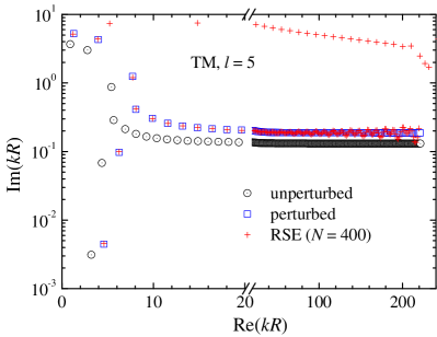
Figure 1: Top: Wave numbers of TM RSs calculated exactly for the unperturbed (black circles with dots) and perturbed system (blue squares), and by solving the RSE equation (24) with $N=400$ RSs in the basis (red crosses). The unperturbed (perturbed) system is a homogeneous dielectric sphere in vacuum, with radius $R$ (0.7$R$), permittivity $\varepsilon=8$ and permeability $\mu=1$. Bottom: Relative error of the RSE calculation of the RS wave numbers for different basis sizes $N$ as given.

As we see from this example, the new version of the RSE with complete elimination of static modes, Eq. (24), has the same slow, $1/N$ convergence to the exact solution as for the standard RSE equation (17) [equivalent to (16) and (18)] with a full set of static modes included LobanovPRA19 . The observed poor convergence of these two quite different versions of the RSE, one with and the other without static modes, has provided us with a sufficient motivation for having a closer look at the dyadic GF, focusing in particular on the properties of its $k=0$ pole, and obtaining different representations of the Green’s dyadic. This has resulted in developing new and more efficient versions of the RSE having a quicker convergence to the exact solution.

In the following sections we consider rigorously the $k=0$ pole of the dyadic GF of spherically symmetric systems and show that the ML forms Eqs. (9) and (19) given above have poor convergence because of the $k=0$ singularity (similar to that in free space LevineCPAM50 ) represented by a series of smooth functions, which are the wave function of the RSs and/or static modes. We then work out alternative ML representations of the Green’s dyadic and following from them RSE equations which have a much quicker convergence. We also provide in Sec. III.5 a rigorous proof of the ML expansions Eqs. (9) and (19) for spherically symmetric systems.

III Spherically symmetric systems

We now concentrate on spherically symmetric systems and use the advantage that the full 3D problem for the RSs and the GF in this case can be reduced to effective 1D where many useful properties can be derived analytically. At the same time, we assume in this section an arbitrary radial dependence of the generalized permittivity, thus keeping all the conclusions made in this work as general as possible. We assume that such a spherically symmetric optical system is finite, having radius $R$, and is surrounded by vacuum, although a generalization of the obtained results to arbitrary uniform permittivity of the surrounding medium is straightforward. Application of these results to a homogeneous sphere allowing explicit analytic solutions will be done in the next section.

For a spherically symmetric system, its permittivity and permeability have only radial dependence,

$$\hat{{\boldsymbol{\varepsilon}}}(\textbf{r})=\hat{\mathbf{1}}\varepsilon(r)\,,\ \ \ \hat{{\boldsymbol{\mu}}}(\textbf{r})=\hat{\mathbf{1}}\mu(r)\,,\ \ \$$

(here, we naturally assume also their isotropy). It is convenient to use vector spherical harmonics (VSHs) $\textbf{Y}_{jlm}(\Omega)$ ($j=1,2,3$) for solving Maxwell’s equations for the RSs and the GF, Eqs. (5) and (3), respectively. The VSHs are defined as

$$\textbf{Y}_{1lm}=\frac{\textbf{r}}{\alpha_{l}}\times\nabla Y_{lm}\,,\ \ \ \textbf{Y}_{2lm}=\frac{r}{\alpha_{l}}\nabla Y_{lm}\,,\ \ \ \textbf{Y}_{3lm}=\frac{\textbf{r}}{r}Y_{lm}\,,$$ (26)

where

$$\alpha_{l}=\sqrt{l(l+1)}\,,$$ (27)

$Y_{lm}(\Omega)$ are scalar spherical harmonics defined in Appendix A, $l$ and $m$ are the spherical quantum numbers, and $\Omega=(\theta,\varphi)$ is the angular part of the standard spherical coordinates. Using the completeness of the VSHs, we consider an expansion of the electric field into the VSHs:

$$\textbf{E}(\textbf{r})=\sum_{jlm}E_{jlm}(r)\textbf{Y}_{jlm}(\Omega)\,.$$ (28)

A similar expression is valid for the magnetic field, mapping $\textbf{H}(\textbf{r})\to H_{jlm}(r)$ . As shown in Appendix A, Maxwell’s equations (1) transform into a $6\times 6$ matrix differential equation for the radial coordinate only, which in turn splits into two separate $3\times 3$ blocks, one block corresponding to TE, the other to TM polarization. The TE block has the following form

$$\left(\begin{array}[]{ccc}k\varepsilon(r)&-\frac{1}{r}\frac{d}{dr}r&\frac{\alpha_{l}}{r}\\ \frac{1}{r}\frac{d}{dr}r&k\mu(r)&0\\ \frac{\alpha_{l}}{r}&0&k\mu(r)\end{array}\right)\left(\begin{array}[]{c}E_{1lm}(r)\\ iH_{2lm}(r)\\ iH_{3lm}(r)\end{array}\right)=0\,,$$ (29)

with $E_{2lm}(r)=E_{3lm}(r)=H_{1lm}(r)=0$. To obtain the corresponding matrix differential equation for TM polarization, one needs to make the following exchange in Eq. (29):

$$E_{jlm}(r)\leftrightarrow iH_{jlm}(r)\,,\ \ \ \varepsilon(r)\leftrightarrow\mu(r)\,.$$ (30)

We therefore consider in the following only solutions for TE polarization, for generality of results keeping $\mu$ where appropriate (even if $\mu=1$ everywhere, which is the case of non-magnetic systems).

Let us introduce new radial functions,

$$\mathcal{E}_{j}(r)=rE_{jlm}(r)\,,\ \ \ \mathcal{H}_{j}(r)=riH_{jlm}(r)\,,$$ (31)

so that Eq. (29) transforms into a simpler form

$$\hat{\mathcal{M}}(k,r)\mathbfcal{F}(r)=0$$ (32)

with

$$\hat{\mathcal{M}}(k,r)=\left(\begin{array}[]{ccc}k\varepsilon(r)&-\frac{d}{dr}&\frac{\alpha}{r}\\ \frac{d}{dr}&k\mu(r)&0\\ \frac{\alpha}{r}&0&k\mu(r)\end{array}\right)$$ (33)

and

$$\mathbfcal{F}(r)=\left(\begin{array}[]{c}\mathcal{E}_{1}(r)\\ \mathcal{H}_{2}(r)\\ \mathcal{H}_{3}(r)\end{array}\right)\,.$$ (34)

Note that for brevity of notations we have also omitted here and almost everywhere below indices $l$ and $m$ (this includes replacing $\alpha_{l}$ with just $\alpha$). Excluding $\mathcal{H}_{2}$ and $\mathcal{H}_{3}$, Eq. (32) transforms into the following differential equation for $\mathcal{E}_{1}$:

$$\hat{L}(k,r)\mathcal{E}_{1}(r)=0\,,$$ (35)

where $\hat{L}(k,r)$ is a 2nd-order differential operator:

$$\hat{L}(k,r)=\mu(r)\frac{d}{dr}\frac{1}{\mu(r)}\frac{d}{dr}-\frac{\alpha^{2}}{r^{2}}+k^{2}\varepsilon(r)\mu(r)\,.$$ (36)

Introducing a 1st-order vector differential operator

$$\hat{O}(k,r)=\left(\begin{array}[]{c}1\\ -\frac{1}{k\mu(r)}\frac{d}{dr}\\ -\frac{\alpha}{kr\mu(r)}\end{array}\right)\,,$$ (37)

the full vectorial solution of Eq. (32) can then be written in the following compact form

$$\mathbfcal{F}(r)=\hat{O}(k,r)\mathcal{E}_{1}(r)\,.$$ (38)

Equation (3) for the GF is transformed using the basis of the VSHs in a very similar way. We first write the full $6\times 6$ GF more explicitly, in terms of four $3\times 3$ blocks,

$$\hat{\mathbb{G}}_{k}(\textbf{r},\textbf{r}^{\prime})=\left(\begin{array}[]{cc}\hat{G}_{k}^{EE}&\hat{G}_{k}^{EH}\\ \hat{G}_{k}^{HE}&\hat{G}_{k}^{HH}\end{array}\right)\,,$$

and then expand each block of the GF into the VSHs. The $EE$ block, for example, is expanded as

$$\hat{G}_{k}^{EE}(\textbf{r},\textbf{r}^{\prime})=\sum_{ij}\sum_{lm}[G^{EE}_{ij}(r,r^{\prime})]_{lm}\textbf{Y}_{ilm}(\Omega)\otimes\textbf{Y}_{jlm}(\Omega^{\prime})\,,$$

where the single summation over $l,m$ is due to the spherical symmetry of the optical system. For the same reason, TE and TM parts of the GF separate from each other, with all the cross terms between different polarizations vanishing. Again, it is sufficient to find a general solution only for one of the two polarizations, then with the exchange Eq. (30) the solution in the other polarization takes exactly the same form. We therefore concentrate in the following on the TE block of the GF, which in the VSH basis has the form

$$\frac{1}{rr^{\prime}}\hat{\mathcal{G}}(r,r^{\prime})\equiv\left(\begin{array}[]{ccc}G_{11}^{EE}&G_{12}^{EH}&G_{13}^{EH}\\ G_{21}^{HE}&G_{22}^{HH}&G_{23}^{HH}\\ G_{31}^{HE}&G_{32}^{HH}&G_{33}^{HH}\end{array}\right)\,.$$

Here, we have introduced for convenience, in full analogy with Eq. (31), a new dyadic GF $\hat{\mathcal{G}}(r,r^{\prime})$ which satisfies the following matrix differential equation:

$$\hat{\mathcal{M}}(k,r)\hat{\mathcal{G}}(r,r^{\prime})=\hat{\mathbf{1}}\delta(r-r^{\prime})\,,$$ (39)

where $\hat{\mathbf{1}}$ is the $3\times 3$ identity matrix. It also follows from the general reciprocity relation Eq. (4) that

$$\mathcal{G}_{ij}(r^{\prime},r)=\mathcal{G}_{ji}(r,r^{\prime})\,.$$ (40)

in which $\mathcal{G}_{ij}$ are the matrix elements of $\hat{\mathcal{G}}$.

III.1 Dyadic Green’s function for fixed $l$ and $m$

First of all, we note that components $\mathcal{G}_{12}$, $\mathcal{G}_{21}$, $\mathcal{G}_{23}$, and $\mathcal{G}_{32}$ of the GF have discontinuities at $r=r^{\prime}$ and component $\mathcal{G}_{33}$ is irregular as it contains a $\delta$ function, as it immediately follows from Eq. (39) – see also Appendix B for details. All other matrix elements of the GF, including the regular part of $\mathcal{G}_{33}$ are continuous and finite for any finite $r$, $r^{\prime}$, and complex $k$ (the same is true also for any component of the GF when $r\neq r^{\prime}$).

It is important to note at this point that the slow convergence of the standard version of the RSE considered in Sec. II.2 is actually caused by the presence of the $\delta$ function in $\mathcal{G}_{33}$ and by the fact that this $\delta$ function is expanded into static modes. Usually, expansions of $\delta$ functions into compete sets of regular smooth functions have very poor convergence. In the second version of the RSE presented in Sec. II.3, this $\delta$ function is eliminated from the ML series. However, the slow convergence in that case is caused by two other $\delta$ functions added to elements $\mathcal{G}_{11}(r,r^{\prime})$ and $\mathcal{G}_{22}(r,r^{\prime})$, respectively. These $\delta$ functions are again represented by expansions, this time in terms of the RSs only, which makes this version of the RSE, from the point of its practical use, essentially similar to the first one.

The solution of Eq. (39) is derived in Appendix B. As in the case of a homogeneous slab Sam19 , the Green’s dyadic can be written in the following compact way, using only the scalar function $\mathcal{G}_{11}(r,r^{\prime})$:

$$\hat{\mathcal{G}}(r,r^{\prime})=\hat{O}(k,r)\otimes\hat{O}(k,r^{\prime})\mathcal{G}_{11}(r,r^{\prime})+\frac{\delta(r-r^{\prime})}{k\mu(r)}(\hat{\mathbf{1}}_{2}+\hat{\mathbf{1}}_{3})$$ (41)

with operator $\hat{O}$ defined by Eq. (37) and $(\hat{\mathbf{1}}_{j})_{ii^{\prime}}=\delta_{ii^{\prime}}\delta_{ij}$. Element $\mathcal{G}_{11}(r,r^{\prime})$ of the dyadic GF satisfies the outgoing wave boundary conditions (for real $k$) and the following ordinary differential equation with a source

$$\hat{L}(k,r)\mathcal{G}_{11}(r,r^{\prime})=k\mu(r)\delta(r-r^{\prime})\,,$$ (42)

where the operator $\hat{L}$ is defined by Eq. (36).

Equation (42) can be easily solved for any spherically symmetric system, analytically (as done in Sec. IV) or numerically. The term $\hat{\mathbf{1}}_{3}\delta(r-r^{\prime})$ in Eq. (41) is the singular part of $\mathcal{G}_{33}(r,r^{\prime})$ discussed above, which a true physical singularity of the dyadic GF. There is however an additional singular term $\hat{\mathbf{1}}_{2}\delta(r-r^{\prime})$ which appears in Eq. (41) in order to compensate on a singularity emerging from second derivative which is appears after applying twice the operator $\hat{O}(k,r)$ – for more details, see Appendix B.

Equation (42) has the following explicit solution:

$$\mathcal{G}_{11}(r,r^{\prime})=\frac{\mathcal{E}_{L}(r_{<})\mathcal{E}_{R}(r_{>})}{W},$$ (43)

where $r_{<}=\min(r,r^{\prime})$, $r_{>}=\max(r,r^{\prime})$, $\mathcal{E}_{L(R)}(r)$ is the so-called left (right) solution, and

$$W=\frac{\mathcal{E}_{L}(r)\mathcal{E}^{\prime}_{R}(r)-\mathcal{E}^{\prime}_{L}(r)\mathcal{E}_{R}(r)}{k\mu(r)}$$ (44)

is the Wronskian, which is independent of $r$. $\mathcal{E}_{L(R)}(r)$ satisfies the corresponding homogeneous equation (35) and the left (right) boundary condition for the GF:

$$\begin{array}[]{ll}\mathcal{E}_{L}(r)\propto r^{l+1}&\ {\rm at}\ r\to 0\,,\\ \mathcal{E}_{R}(r)\propto rh^{(1)}_{l}(kr)&\ {\rm at}\ r>R\,.\end{array}$$ (45)

The first condition follows from the asymptotic behaviour of the operator Eq. (35) at small $r$ and the regularity of the GF at the origin, while the second one is the outgoing boundary condition, assuming a constant refractive index outside the system, e.g. $\varepsilon(r)\mu(r)=1$. Here, $h^{(1)}_{l}(z)$ is the spherical Hankel function of 1st kind. Introducing the corresponding vector functions,

$$\mathbfcal{F}_{L(R)}(r)=\hat{O}(k,r)\mathcal{E}_{L(R)}(r)$$ (46)

with $\hat{O}$ given by Eq. (37), the full dyadic GF takes the following form

$$\hat{\mathcal{G}}(r,r^{\prime})=\frac{\delta(r-r^{\prime})}{k\mu(r)}\hat{\mathbf{1}}_{3}+\frac{1}{W}\times\left\{\begin{array}[]{ll}\mathbfcal{F}_{L}(r)\otimes\mathbfcal{F}_{R}(r^{\prime})&r<r^{\prime}\\ \mathbfcal{F}_{R}(r)\otimes\mathbfcal{F}_{L}(r^{\prime})&r>r^{\prime}\,,\end{array}\right.$$ (47)

where the singular term $\hat{\mathbf{1}}_{2}\delta(r-r^{\prime})$, previously added to Eq. (41), has now been removed, while the real, physical singularity of the dyadic GF remains. It is represented by the 1st term in Eq. (47), clearly contributing to the static, $k=0$ pole of the GF. The 2nd term in Eq. (47) contains no spatial singularities, but it also brings in a significant contribution to the static pole of the GF, as we show in Sec. III.2 below.

III.2 Static pole of the dyadic GF

To study the behaviour of the dyadic GF in the static limit and to find its residue at the $k=0$ pole, we introduce an auxiliary, $k$-independent matrix $\mathcal{R}_{ij}$ defined in such a way that

$$\hat{\mathcal{G}}(r,r^{\prime})\to\frac{1}{k}\left(\begin{array}[]{ccc}k^{2}\mathcal{R}_{11}&k\mathcal{R}_{12}&k\mathcal{R}_{13}\\ k\mathcal{R}_{21}&\mathcal{R}_{22}&\mathcal{R}_{23}\\ k\mathcal{R}_{31}&\mathcal{R}_{32}&\mathcal{R}_{33}\end{array}\right)$$ (48)

at $k\to 0$. Substituting Eq. (48) into Eq. (39) and taking the limit $k\to 0$, we find the following differential equation for matrix $\mathcal{R}_{ij}$:

$$\left(\begin{array}[]{ccc}0&-\frac{d}{dr}&\frac{\alpha}{r}\\ \frac{d}{dr}&\mu&0\\ \frac{\alpha}{r}&0&\mu\end{array}\right)\left(\begin{array}[]{ccc}\mathcal{R}_{11}&\mathcal{R}_{12}&\mathcal{R}_{13}\\ \mathcal{R}_{21}&\mathcal{R}_{22}&\mathcal{R}_{23}\\ \mathcal{R}_{31}&\mathcal{R}_{32}&\mathcal{R}_{33}\end{array}\right)=\hat{\mathbf{1}}\delta(r-r^{\prime})\,,$$ (49)

which is looking similar to Eq. (39). Solving it in a similar way (see Appendix B for details), we find the residue of the dyadic GF at $k=0$:

$$\hat{\mathcal{R}}(r,r^{\prime})\equiv\left(\begin{array}[]{ccc}0&0&0\\ 0&\mathcal{R}_{22}&\mathcal{R}_{23}\\ 0&\mathcal{R}_{32}&\mathcal{R}_{33}\end{array}\right)=-rr^{\prime}\hat{\nabla}(r)\otimes\hat{\nabla}(r^{\prime})g(r,r^{\prime})$$ (50)

(note that matrices $\hat{\mathcal{R}}$ and $\mathcal{R}_{ij}$ are not the same!). In the VSH basis, the gradient operator has the form

$$\hat{\nabla}(r)=\left(\begin{array}[]{c}0\\ \frac{\alpha}{r}\\ \frac{d}{dr}\end{array}\right)\,,$$ (51)

which is derived in Appendix A. The new scalar GF $g(r,r^{\prime})$ introduced in Eq. (50) satisfies the following equation

$$\left[\frac{1}{r^{2}\mu(r)}\frac{d}{dr}r^{2}\mu(r)\frac{d}{dr}-\frac{\alpha^{2}}{r^{2}}\right]g(r,r^{\prime})=\frac{\delta(r-r^{\prime})}{r^{2}\mu(r)}$$ (52)

and the boundary conditions that $g(r,r^{\prime})$ is regular at $r,r\to 0$ and vanishing at $r,r^{\prime}\to\infty$. Element $\mathcal{R}_{33}$ has a singularity equivalent to the first term in Eq. (47). In the solution given by Eq. (50) this singularity is technically generated by the second mixed derivative of $g(r,r^{\prime})$ – see Appendix B for details.

Interestingly, by varying the equation for the scalar GF, such as Eq. (52) for $g(r,r^{\prime})$, the residue of the dyadic GF at the $k=0$ pole takes alternative representations, different from Eq. (50), as discussed in more depths in Secs. III.5 and IV.3 below and at the end of Appendix C. Here we give one more representation, also derived in Appendix B, which provides a natural link to the regular element $\mathcal{G}_{11}$ of the dyadic GF in the limit $k\to 0$:

$$\hat{\mathcal{R}}(r,r^{\prime})=\hat{Q}(r)\otimes\hat{Q}(r^{\prime})\tilde{g}(r,r^{\prime})+\frac{\delta(r-r^{\prime})}{\mu(r)}(\hat{\mathbf{1}}_{2}+\hat{\mathbf{1}}_{3})\,,$$ (53)

where we have introduced a new operator

$$\hat{Q}(r)=\lim_{k\to 0}k\hat{O}(k,r)=-\frac{1}{\mu(r)}\left(\begin{array}[]{c}0\\ \frac{d}{dr}\\ \frac{\alpha}{r}\end{array}\right)$$ (54)

and a new scalar GF $\tilde{g}(r,r,^{\prime})$ satisfying an equation

$$\left[\mu(r)\frac{d}{dr}\frac{1}{\mu(r)}\frac{d}{dr}-\frac{\alpha^{2}}{r^{2}}\right]\tilde{g}(r,r^{\prime})=\mu(r)\delta(r-r^{\prime})$$ (55)

and the same boundary conditions as ${g}(r,r^{\prime})$. Since the operator in the square brackets in Eq. (55) is $\hat{L}(0,r)$ [see Eq. (36)], we find

$$\tilde{g}(r,r^{\prime})=\lim_{k\to 0}\frac{\mathcal{G}_{11}(r,r^{\prime})}{k}\,,$$ (56)

in agreement with Eq. (42). In fact, the outgoing boundary condition for $\mathcal{G}_{11}(r,r^{\prime})$ transforms in the limit $k\to 0$ into the vanishing boundary condition for $\tilde{g}(r,r^{\prime})$ at $r,r^{\prime}\to\infty$, owing to the asymptotic behaviour of the Hankel functions at a vanishing argument. Similar to Eq. (41), representation Eq. (53) of the static-pole residue of the GF introduces an additional explicit singularity $\hat{\mathbf{1}}_{2}\delta(r-r^{\prime})/\mu(r)$ which is exactly compensated by the second mixed derivative in $\mathcal{R}_{22}$.

III.3 Static modes

The scalar GF $g$ or $\tilde{g}$, defined by Eqs. (52) or (55), respectively, determines a complete set of static modes which can be used for expansion of the $k=0$ residue of the dyadic GF. Note that with a replacement $r^{2}\mu(r)\to 1/\mu(r)$, Eq. (52) transforms into Eq. (55). Let us therefore introduce a general second-order differential operator

$$\hat{\cal L}(r)=\frac{1}{w(r)}\frac{d}{dr}w(r)\frac{d}{dr}-\frac{\alpha^{2}}{r^{2}}\,,$$ (57)

where $w(r)$ is some weight function. This operator generates an eigenvalue equation

$$\left[\hat{\cal L}(r)+\lambda^{2}\Theta(R-r)\right]\phi_{\lambda}(r)=0\,,$$ (58)

where $\Theta(x)$ is the Heaviside step function. The corresponding GF $G_{\Lambda}(r,r^{\prime})$ satisfies an equation

$$\left[\hat{\cal L}(r)+\Lambda\Theta(R-r)\right]G_{\Lambda}(r,r^{\prime})=\frac{\delta(r-r^{\prime})}{w(r)}\,.$$ (59)

Here, both $\phi_{\lambda}$ and $G_{\Lambda}$ obey vanishing boundary conditions at $r,r^{\prime}\to\infty$ and regularity at the origin. Note that $\lambda$ in Eq. (58) is the eigenvalue, while $\Lambda$ in Eq. (59) is a parameter which can take any value. Multiplying Eq. (58) with $\phi_{\lambda^{\prime}}w$, integrating the result over the full space, and then subtracting from it the same equation with $\lambda$ and $\lambda^{\prime}$ interchanged, we obtain an orthogonality relation

$$(\lambda^{2}-\lambda^{\prime 2})\int_{0}^{R}\ \phi_{\lambda}(r)\ \phi_{\lambda^{\prime}}(r)w(r)dr=0\,.$$

Then using the completeness of the set of functions $\phi_{\lambda}(r)$ and the symmetry of the GF, $G_{\Lambda}(r,r^{\prime})=G_{\Lambda}(r^{\prime},r)$, we obtain the following spectral representation

$$G_{\Lambda}(r,r^{\prime})=\sum_{\lambda}\frac{\phi_{\lambda}(r)\phi_{\lambda}(r^{\prime})}{\Lambda-\lambda^{2}}\,,$$ (60)

valid within the system, i.e. for $r\leqslant R$. Substituting it into Eq. (59) and using Eq. (58), we obtain a closure relation

$$w(r)\Theta(R-r)\sum_{\lambda}{\phi_{\lambda}(r)\phi_{\lambda}(r^{\prime})}=\delta(r-r^{\prime})\,,$$

confirming the completeness of the basis $\{\phi_{\lambda}\}$ within the system, and a normalization condition

$$\int_{0}^{R}\ \phi_{\lambda}(r)\ \phi_{\lambda^{\prime}}(r)w(r)dr=\delta_{\lambda\lambda^{\prime}}\,,$$ (61)

which is combined here with the already proven orthogonality.

The scalar GF $g(r,r^{\prime})$ contributing to the static pole of the dyadic GF via Eq. (50) is then given by a static-mode expansion

$$g(r,r^{\prime})=G_{0}(r,r^{\prime})=-\sum_{\lambda}\frac{\phi_{\lambda}(r)\phi_{\lambda}(r^{\prime})}{\lambda^{2}}$$ (62)

with the static-mode basis $\{\phi_{\lambda}\}$ generated by Eqs. (57) and (58) with $w(r)=r^{2}\mu(r)$. In the case of a homogeneous sphere in vacuum, this basis, called volume-charge (VC) static-mode basis, was introduced in LobanovPRA19 and applied there successfully for treating both spherical and non-spherical systems.

III.4 Resonant states and their normalization

The wave function of RS $n$ is given by Eq. (38) with $k=k_{n}$ and $\mathbfcal{F}(r)=\mathbfcal{F}_{n}(r)$. The complex eigen wave number $k_{n}$ and the first component of the vectorial wave function $\mathcal{E}_{1}$ are solutions of the wave equation (35) with outgoing boundary conditions. From the general normalization of the RSs, Eq. (II.1), we find, using the properties of the VSHs Eqs. (108) and (109) and integration by parts, the RS normalization:

$$1 = \int_{0}^{R}(\varepsilon\mathcal{E}_{1}^{2}+\mu\mathcal{H}_{2}^{2}+\mu\mathcal{H}_{3}^{2})dr+\frac{R}{k_{n}}\left.\left(\mathcal{H}_{2}\mathcal{E}_{1}^{\prime}-\mathcal{E}_{1}\mathcal{H}_{2}^{\prime}\right)\right|_{r=R_{+}}$$ (63)

$$= 2\int_{0}^{R}\varepsilon\mathcal{E}_{1}^{2}dr+\frac{1}{k_{n}}\left[\left(\mathcal{E}_{1}\frac{r}{\mu(r)}\mathcal{E}_{1}^{\prime}\right)^{\prime}-\frac{2r}{\mu(r)}(\mathcal{E}_{1}^{\prime})^{2}\right]_{r=R_{+}}$$

where the prime means $d/dr$ and $R_{+}=R+0_{+}$ with a positive infinitesimal $0_{+}$. Note that, the second line in Eq. (63) presents exactly the same form of the RS normalization as was derived in MuljarovEPL10 for $\mu=1$, apart from the factor of 2 introduced later on in MuljarovOL18 .

III.5 Mittag-Leffler series for the Green’s dyadic

For its use in the RSE, the GF should have a dyadic product form. Such a product form is provided by applying the ML theorem Arfken01 . Thanks to reciprocity, the RS poles of the GF contribute in a form of dyadic products of the corresponding RS fields $\mathbfcal{F}_{n}(r)$:

$$\hat{\mathcal{G}}(r,r^{\prime}) = \sum_{n}\frac{\mathbfcal{F}_{n}(r)\otimes\mathbfcal{F}_{n}(r^{\prime})}{k-k_{n}}+\frac{\hat{\mathcal{R}}(r,r^{\prime})}{k}\,.$$ (64)

As for the static pole of the dyadic GF, its residue $\hat{\mathcal{R}}(r,r^{\prime})$ introduced and studied in Sec. III.2 does not have a dyadic product form and therefore needs to be expanded into some basis states, which is done below. In this section, we introduce and discuss three different ML representations of the dyadic GF. One more ML representation, with static-mode elimination, is provided in Sec. IV and illustrated in Sec. V, in comparison with other versions.

1st ML representation

Since the full dyadic GF $\hat{\mathcal{G}}(r,r^{\prime})$ can be expressed in terms of its first element, as given by Eq. (41), we concentrate here on finding a ML series for $\mathcal{G}_{11}(r,r^{\prime})$, a scalar GF satisfying Eq. (42) and outgoing boundary conditions. Equation (42) contains the same operator $\hat{L}$, given by Eq. (36), as appears in the wave equation (35) determining the electric field of the RSs in TE polarization:

$$\hat{L}(k_{n},r)\mathcal{E}_{n}(r)=0\,.$$ (65)

Here we use for convenience index $n$ labelling the RSs, so that $\mathcal{E}_{1}$ is replaced with $\mathcal{E}_{n}$. Treating $\mathcal{G}_{11}(r,r^{\prime})$ as a function in the complex $k$-plane, we note that, thanks to Eq. (65), it has simple poles at $k=k_{n}$. Also, it vanishes as $1/k$ at large $k$, as it follows from Eq. (42). Calculating the residues at the poles and then applying the ML theorem Arfken01 to $\mathcal{G}_{11}$, we find the following series representation:

$$\mathcal{G}_{11}(r,r^{\prime})=\sum_{n}\frac{\mathcal{E}_{n}(r)\mathcal{E}_{n}(r^{\prime})}{k-k_{n}}\,,$$ (66)

where the field $\mathcal{E}_{n}(r)$ is normalized according to Eq. (63). The proof of Eq. (66) is very similar to that provided for non-magnetic systems in the Appendix of Ref. MuljarovEPL10 ; we therefore do not repeat it in this paper.

Taking into account the fact that the dyadic GF $\hat{\mathcal{G}}(r,r^{\prime})$ has only simple poles at the RS wave numbers, $k=k_{n}$, and at $k=0$, as expressed by Eq. (64), we substitute the scalar ML expansion Eq. (66) into the general form of the dyadic GF, Eq. (41). Comparing the result with Eq. (64), this leads to

$$\mathbfcal{F}_{n}(r)=\hat{O}(k_{n},r)\mathcal{E}_{n}(r)\,,$$ (67)

which is identical to Eq. (38) [the operator $\hat{O}(k,r)$ is defined in Eq. (37)], provided that $\mathcal{E}_{1}(r)$ in Eq. (38) is the RS field normalized according to Eq. (63).

As for the $k=0$ pole, its residue is given by Eq. (50), where the scalar GF $g(r,r^{\prime})$ may be used in the form of the series Eq. (62). This results in the 1st ML representation of the dyadic GF:

$$\hat{\mathcal{G}}(r,r^{\prime})=\sum_{n}\frac{\mathbfcal{F}_{n}(r)\otimes\mathbfcal{F}_{n}(r^{\prime})}{k-k_{n}}+\sum_{\lambda}\frac{\mathbfcal{F}_{\lambda}(r)\otimes\mathbfcal{F}_{\lambda}(r^{\prime})}{k}\,,$$ (68)

where the LM static-mode fields are given by

$$\mathbfcal{F}_{\lambda}(r)=-r\hat{\nabla}(r)\psi_{\lambda}(r)=-\left(\begin{array}[]{c}0\\ \alpha\psi_{\lambda}(r)\\ {r}\frac{d}{dr}\psi_{\lambda}(r)\end{array}\right)\,,$$ (69)

in accordance with Eqs. (7) and (51). Here, $\psi_{\lambda}(r)=\phi_{\lambda}(r)/\lambda$, and $\phi_{\lambda}(r)$ are the normalized eigen solutions of Eq. (58) with $w(r)=r^{2}\mu(r)$.

The 1st ML representation given by Eq. (68) is identical to the general ML series Eq. (9) introduced at the beginning of Sec. II, which was also used for the conventional RSE in DoostPRA14 ; LobanovPRA19 , though without any rigorous treatment of the static pole. Such a rigorous treatment and a proof of Eq. (9) for spherically symmetric systems have now been provided above.

2nd ML representation

It is also useful to apply the ML theorem to function $\mathcal{G}_{11}(r,r^{\prime})/k$ which vanishes at $k\to\infty$ quicker than $\mathcal{G}_{11}$ and takes a finite value at $k\to 0$. In fact, $\mathcal{G}_{11}$ is vanishing linearly in $k$ at $k\to 0$ as can be seen from Eq. (42). The ML series then takes the form

$$\frac{1}{k}\mathcal{G}_{11}(r,r^{\prime})=\sum_{n}\frac{\mathcal{E}_{n}(r)\mathcal{E}_{n}(r^{\prime})}{k_{n}(k-k_{n})}\,.$$ (70)

Clearly, this series has a quicker convergence compared to its counterpart in Eq. (66), due to the fact that $k_{n}\propto n$ at large $n$, which is a general property of Fabry-Pérot modes in any optical system.

Substituting the series Eq. (70) for the GF into Eq. (42) and using Eq. (65), we obtain a closure relation,

$$\varepsilon(r)\sum_{n}\mathcal{E}_{n}(r)\mathcal{E}_{n}(r^{\prime})=\delta(r-r^{\prime})\,,$$ (71)

and a sum rule,

$$\sum_{n}\frac{\mathcal{E}_{n}(r)\mathcal{E}_{n}(r^{\prime})}{k_{n}}=0\,,$$ (72)

which is equivalent to the fact that $\mathcal{G}_{11}$ vanishes at $k=0$, as noted above – see also Eq. (66). Function $\mathcal{G}_{11}/k$ is in turn finite and $\mathcal{G}_{11}/k^{2}$ has a simple pole at $k=0$. Applying the ML theorem again, this time to $\mathcal{G}_{11}/k^{2}$, we obtain

$$\frac{1}{k^{2}}\mathcal{G}_{11}(r,r^{\prime})=\sum_{n}\frac{\mathcal{E}_{n}(r)\mathcal{E}_{n}(r^{\prime})}{k^{2}_{n}(k-k_{n})}-\frac{1}{k}\sum_{n}\frac{\mathcal{E}_{n}(r)\mathcal{E}_{n}(r^{\prime})}{k^{2}_{n}}\,,$$ (73)

where the last term is noting else than $\tilde{g}(r,r^{\prime})/k$, see Eqs. (56) and (70). The series representations given by Eqs. (66), (70), and (73) allow us to use the general solution Eqs. (41) and (53), for deriving a new ML series for the full dyadic GF. Using all three representations of $\mathcal{G}_{11}(r,r^{\prime})$, we first obtain

$$\hat{O}(k,r)\otimes\hat{O}(k,r^{\prime})\mathcal{G}_{11}(r,r^{\prime})$$

$$=\sum_{n}\frac{\hat{O}(k_{n},r)\mathcal{E}_{n}(r)\otimes\hat{O}(k_{n},r^{\prime})\mathcal{E}_{n}(r^{\prime})}{k-k_{n}}$$

$$-\frac{1}{k}\sum_{n}\frac{\hat{Q}(r)\mathcal{E}_{n}(r)\otimes\hat{Q}(r^{\prime})\mathcal{E}_{n}(r^{\prime})}{k^{2}_{n}}\,,$$ (74)

where the operators $\hat{O}(k,r)$ and $\hat{Q}(r)$ are given, respectively, by Eqs. (37) and (54). Note that the operator $\hat{Q}(r)/k_{n}$ is the same as $\hat{O}(k_{n},r)$, apart from the first element which is vanishing in $\hat{Q}(r)$. In the second, static-pole series in Eq. (74), this operator can be upgraded to $\hat{O}(k_{n},r)$, by adding required terms to one diagonal and four off-diagonal elements of the dyadic GF. The terms added to the off-diagonal elements are however all vanishing, owing to the sum rule Eq. (72), while the term added to the diagonal element $\mathcal{G}_{11}$ can be converted into a $\delta$ function, thanks to the closure relation Eq. (71). We therefore find a ML series for the dyadic GF in the following form:

$$\hat{\mathcal{G}}(r,r^{\prime}) = \sum_{n}\frac{\mathbfcal{F}_{n}(r)\otimes\mathbfcal{F}_{n}(r^{\prime})}{k-k_{n}}-\frac{1}{k}\sum_{n}{\mathbfcal{F}_{n}(r)\otimes\mathbfcal{F}_{n}(r^{\prime})}$$ (75)

$$+\left[\frac{\hat{\mathbf{1}}_{1}}{\varepsilon(r)}+\frac{\hat{\mathbf{1}}_{2}+\hat{\mathbf{1}}_{3}}{\mu(r)}\right]\frac{\delta(r-r^{\prime})}{k}\,,$$

where $\mathbfcal{F}_{n}(r)$ is given by Eq. (67).

The 2nd ML representation given by Eq. (75) has no contribution of static modes and is equivalent to the general ML series Eq. (19) introduced in Sec. II. As it is shown in the example provided in Sec. II.3 above, the RSE based on this series has a rather slow convergence – see also a comparison in Sec. V below.

3rd ML representation

In fact, the second series in Eq. (75) is very inefficient for representing elements $\mathcal{G}_{11}$ and $\mathcal{G}_{22}$ as it contains $\delta$ functions for both, expanded into sets of smooth functions. While the $\delta$ function in $\mathcal{G}_{11}$ was added by hand, as described above, and thus can be easily removed, as done below, the static pole series for $\mathcal{G}_{22}$ has a poor convergence due to the mixed second-order partial derivative, which also implicitly contains a $\delta$ function. To improve on this, we fist subtract in Eq. (75) the entire $k=0$ pole from $\mathcal{G}_{22}$, which is given by

$$\frac{\delta(r-r^{\prime})}{k\mu(r)}\hat{\mathbf{1}}_{2}-\frac{1}{k\mu(r)\mu(r^{\prime})}\sum_{n}\frac{\mathcal{E}^{\prime}_{n}(r)\mathcal{E}^{\prime}_{n}(r^{\prime})}{k_{n}^{2}}\hat{\mathbf{1}}_{2}\,,$$ (76)

with a singularity in the second term exactly compensating the $\delta$ function in the first one. We then add a regular representation of the $k=0$ pole of $\mathcal{G}_{22}$, given by an expression

$$-\frac{\alpha^{2}}{k}g(r,r^{\prime})\hat{\mathbf{1}}_{2}$$ (77)

provided by the static-pole analysis of the GF, see Eqs. (50) and (114).

For the full GF to have a dyadic product form, we need to expand Eq. (77) into a complete set of functions. This can be any set which is complete within the system volume, $r\leqslant R$. The second-order differential operator Eq. (57) with $w(r)=r^{2}\mu(r)$ naturally generates such a basis, leading to Eq. (62). Using this result, the full dyadic GF then takes the form:

$$\hat{\mathcal{G}}(r,r^{\prime}) = \sum_{n}\frac{\mathbfcal{F}_{n}(r)\otimes\mathbfcal{F}_{n}(r^{\prime})}{k-k_{n}}+\hat{\mathbf{1}}_{3}\frac{\delta(r-r^{\prime})}{k\mu(r)}$$ (78)

$$-\frac{1}{k}\sum_{n}\frac{\hat{Q}(r)\mathcal{E}_{n}(r)\otimes\hat{Q}(r^{\prime})\mathcal{E}_{n}(r^{\prime})}{k_{n}^{2}}$$

$$+\frac{\hat{\mathbf{1}}_{2}}{k}\sum_{n}\frac{\hat{Q}_{2}(r)\mathcal{E}_{n}(r)\hat{Q}_{2}(r^{\prime})\mathcal{E}_{n}(r^{\prime})}{k_{n}^{2}}$$

$$+\hat{\mathbf{1}}_{2}\frac{\alpha^{2}}{k}\sum_{\lambda}\psi_{\lambda}(r)\psi_{\lambda}(r^{\prime})\,,$$

in which the second and the third series, when taken together, do not contain a singularity and are thus converging well, i.e. without an additional static-pole singularity error, in the same way as the first and the last series. Here, $\hat{Q}_{2}(r)=-\mu^{-1}(r)d/dr$ is the second element of the vectorial operator $\hat{Q}(r)$. Equation (78) is the 3rd ML representation provided in this paper. It contains an efficient summations over the RSs and static modes and thus should lead to a quicker version of the RSE, which is derived in Sec. III.6 below. The 3rd ML representation can be written in a more compact way by introducing general vectorial basis functions ${\boldsymbol{\Psi}}_{j}(r)$ representing the static pole:

$$\hat{\mathcal{G}}(r,r^{\prime}) = \sum_{n}\frac{\mathbfcal{F}_{n}(r)\otimes\mathbfcal{F}_{n}(r^{\prime})}{k-k_{n}}+\hat{\mathbf{1}}_{3}\frac{\delta(r-r^{\prime})}{k\mu(r)}$$ (79)

$$+\frac{1}{k}\sum_{j}{\boldsymbol{\Psi}}_{j}(r)\otimes{\boldsymbol{\Psi}}_{j}(r^{\prime})\,,$$

where index $j$ is running over all static modes ($\lambda$) once and over all the RSs ($n$) twice, as it is clear from Eq. (78).

We note that the 3rd ML representation given by Eq. (78) is not unique, and not only in the sense that different sets of static modes can be used, as mentioned above – see also LobanovPRA19 where two different sets were used and Appendix C in which three different sets of static mode are considered. In Sec. IV below we present one more ML representation of the Green’s dyadic, having the same form as given by the more general Eq. (79). This 4th ML representation, suited for a homogeneous sphere, is focusing again on a complete elimination of static modes from the basis and developing a version of the RSE which is based on the RSs only. Elimination of static modes is the main focus of this paper. Therefore, applying the RSE based on the 3rd ML representation Eq. (78) containing different sets of static modes will be done elsewhere.

III.6 Resonant-state expansion

In the basis of the VSHs, Maxwell’s equations (14) for the perturbed system with spherical symmetry, for TE polarization and $l$ and $m$ fixed, reduce to

$$\left[\hat{\cal M}(k,r)+k\Delta\hat{\mathcal{P}}(r)\right]\mathbfcal{F}(r)=0\,,$$ (80)

where $\hat{\cal M}(k,r)$ is defined in Eq. (33), and

$$\Delta\hat{\mathcal{P}}(r)=\left(\begin{array}[]{ccc}\Delta\varepsilon(r)&0&0\\ 0&\Delta\mu(r)&0\\ 0&0&\Delta\mu(r)\end{array}\right)$$ (81)

is the perturbation of the generalized permittivity within the sphere of radius $R$ containing the system. Here $k$ is the eigen wave number, and Eqs. (28), (31), and (34) define the components of the vector field $\mathbfcal{F}(r)$ of a perturbed RS. The solution of Eq. (80) in terms of the dyadic GF is given by

$$\mathbfcal{F}(r)=-k\int_{0}^{R}\hat{\mathcal{G}}(r,r^{\prime})\Delta\hat{\mathcal{P}}(r^{\prime})\mathbfcal{F}(r^{\prime})dr^{\prime}\,.$$

Using Eq. (79), we then find for the perturbed RS field:

$$\hat{\mathcal{D}}^{-1}(r)\mathbfcal{F}(r)=\sum_{n}a_{n}\mathbfcal{F}_{n}(r)+\sum_{j}b_{j}{\boldsymbol{\Psi}}_{j}(r)\,,$$

where

$$\hat{\mathcal{D}}^{-1}(r)=\hat{\mathbf{1}}+\frac{\Delta\mu(r)}{\mu(r)}\hat{\mathbf{1}}_{3}\,.$$

The expansion coefficients have the form

$$a_{n} = -\frac{k}{k-k_{n}}\int_{0}^{R}\mathbfcal{F}_{n}(r)\cdot\Delta\hat{\mathcal{P}}(r)\mathbfcal{F}(r)dr$$ (82)

$$= -\frac{k}{k-k_{n}}\left(\sum_{n^{\prime}}V_{nn^{\prime}}a_{n^{\prime}}+\sum_{j^{\prime}}V_{nj^{\prime}}b_{j^{\prime}}\right)\,,$$

$$b_{j} = -\int_{0}^{R}{\boldsymbol{\Psi}}_{j}(r)\cdot\Delta\hat{\mathcal{P}}(r)\mathbfcal{F}(r)dr$$ (83)

$$= -\sum_{n^{\prime}}V_{jn^{\prime}}a_{n^{\prime}}-\sum_{j^{\prime}}V_{jj^{\prime}}b_{j^{\prime}}\,,$$

where the matrix elements are given by

$$\left(\begin{array}[]{cc}V_{nn^{\prime}}&V_{nj^{\prime}}\\ V_{jn^{\prime}}&V_{jj^{\prime}}\end{array}\right)=\int_{0}^{R}dr\left(\begin{array}[]{c}\mathbfcal{F}_{n}\\ {\boldsymbol{\Psi}}_{j}\end{array}\right)\cdot\Delta\hat{\mathcal{P}}\hat{\mathcal{D}}\left(\begin{array}[]{cc}\mathbfcal{F}_{n^{\prime}}&{\boldsymbol{\Psi}}_{j^{\prime}}\end{array}\right)$$ (84)

with

$$\Delta\hat{\mathcal{P}}\hat{\mathcal{D}}=\Delta\varepsilon(r)\hat{\mathbf{1}}_{1}+\Delta\mu(r)\hat{\mathbf{1}}_{2}+\frac{\mu(r)\Delta\mu(r)}{\mu(r)+\Delta\mu(r)}\hat{\mathbf{1}}_{3}\,.$$

Expressing the static amplitudes from Eq. (83),

$$b_{j}=-\sum_{j^{\prime}}W_{jj^{\prime}}\sum_{n}V_{j^{\prime}n}a_{n}\,,$$

Eq. (82) is transformed to the following matrix equation of the RSE:

$$(k-k_{n})a_{n}=-k\sum_{n^{\prime}}\tilde{V}_{nn^{\prime}}a_{n^{\prime}}\,,$$ (85)

where

$$\tilde{V}_{nn^{\prime}}={V}_{nn^{\prime}}-\sum_{jj^{\prime}}V_{nj}W_{jj^{\prime}}V_{j^{\prime}n^{\prime}}\,,$$

$W_{jj^{\prime}}$ is the inverse of matrix $\delta_{jj^{\prime}}+V_{jj^{\prime}}$, and $n$ labels all the basis RSs. Again, Eq. (85) can be symmetrized, as done at the end of Sec. II.2.

For non-spherical perturbations which can mix states with different spherical numbers ($l,\,m$) and different polarizations, the formalism of the RSE and the key equation (85) remain essentially the same. The difference should appear in the matrix elements Eq. (84) which may be non-vanishing between TE and TM polarizations and between states with different pairs of ($l,\,m$) and ($l^{\prime},\,m^{\prime}$). Applying the RSE to such systems will be the subject of forthcoming publications.

IV Application to a homogeneous sphere in vacuum

We now apply the formalism developed in Sec. III to a homogeneous sphere in vacuum, for its further use as the basis system in the RSE. The system is described by uniform permittivity $\varepsilon$ and permeability $\mu$ for $r\leqslant R$, where $R$ is the radius of the sphere, so that in the entire space

$$\varepsilon(r)=1+(\varepsilon-1)\Theta(R-r)\,,$$

$$\mu(r)=1+(\mu-1)\Theta(R-r)\,.$$

It is useful to introduce at this point the refractive index $n_{r}$ and the impedance $\beta$ of the sphere defined as

$$n_{r}=\sqrt{\varepsilon\mu}\,,\ \ \ \ \beta=\sqrt{\varepsilon/\mu}\,,$$ (86)

respectively, as both quantities contribute to the results obtained below.

Again, we concentrate in this section on TE polarization with fixed spherical quantum numbers $l$ and $m$. All results for TM polarization will then be exactly the same, provided that the replacement Eq. (30) is performed.

IV.1 Analytic form of the dyadic Green’s function

The analytic form of the dyadic GF is given by Eqs. (46) and (47), in terms of the left and right solutions, $\mathcal{E}_{L,R}$. These have the following explicit form for the homogeneous sphere:

$$\begin{array}[]{l}\mathcal{E}_{L}(r;k)=\left\{\begin{array}[]{ll}J(n_{r}kr)&\ r\leqslant R\\ B_{1}J(kr)+B_{2}H(kr)&\ r>R\,,\end{array}\right.\vskip 3.0pt plus 1.0pt minus 1.0pt\\ \mathcal{E}_{R}(r;k)=\left\{\begin{array}[]{ll}CJ(n_{r}kr)+H(n_{r}kr)&r\leqslant R\\ B_{3}H(kr)&r>R\,,\end{array}\right.\end{array}$$ (87)

where $J(z)\equiv zj_{l}(z)$ and $H(z)\equiv zh_{l}^{(1)}(z)$, with $j_{l}(z)$ and $h_{l}^{(1)}(z)$ being, respectively, the spherical Bessel function and Hanken function of first kind. The $k$-dependent coefficients $C$, $B_{1}$, $B_{2}$, and $B_{3}$ in Eq. (87) are found by applying Maxwell’s boundary conditions at $r=R$ and are provided in Appendix C.

The Wronskian Eq. (44) contributing to the dyadic GF Eq. (47) is given by $W=i\beta$, see Eq. (119), and the left and right vector functions Eq. (46) have the following form inside the sphere ($r\leqslant R$):

$$\mathbfcal{F}_{L}(r;k) = \left(\begin{array}[]{c}J(x)\\ -\beta J^{\prime}(x)\\ -\alpha\beta J(x)/x\end{array}\right)\,,$$ (91)

$$\mathbfcal{F}_{R}(r;k) = C(k)\mathbfcal{F}_{L}(r;k)+\left(\begin{array}[]{c}H(x)\\ -\beta H^{\prime}(x)\\ -\alpha\beta H(x)/x\end{array}\right)$$ (95)

with $x=n_{r}kr$, $\alpha$ defined by Eq. (27), $C(k)$ given by Eq. (118), and primes meaning the derivatives of functions with respect to their arguments.

IV.2 Resonant states and their normalization

The RS wave numbers $k_{n}$ are given by the poles of the coefficient $C(k)=N(k)/D(k)$, see Eq. (118). Its denominator $D(k)$ thus determines the secular equation of the RSs in TE polarization:

$$D(k_{n})=\beta H(z)J^{\prime}(n_{r}z)-H^{\prime}(z)J(n_{r}z)=0\,,$$ (96)

where $z=k_{n}R$. The RS wave functions which are given by Eq. (67) then take the form:

$$\mathbfcal{F}_{n}(r)\equiv\left(\begin{array}[]{c}\mathcal{E}_{n}(r)\\ \mathcal{K}_{n}(r)\\ \mathcal{N}_{n}(r)\end{array}\right)=A_{n}\left(\begin{array}[]{c}J(x)\\ -\beta J^{\prime}(x)\\ -\alpha\beta J(x)/x\end{array}\right)\,,$$ (97)

where $x=n_{r}k_{n}r$ ($r\leqslant R$) and $A_{n}$ are the normalization constants. The latter can be found by using the general normalization Eq. (63) or by calculating the residue at $k=k_{n}$ pole of the analytic GF:

$${A_{n}^{2}}=\frac{1}{i\beta}\lim_{k\to k_{n}}(k-k_{n})C(k)\,,$$ (98)

see Eq. (47). Both ways are demonstrated in Appendix C, leading to the same result: $A_{n}={\cal A}(n_{r}k_{n}R)$, where function ${\cal A}(z)$ is defined as

$$\frac{1}{{\cal A}^{2}(z)R}=(\varepsilon-1)J^{2}(z)+\varepsilon(\mu-1)\left[\frac{\alpha^{2}}{z^{2}}J^{2}(z)+\frac{1}{\mu}J^{\prime 2}(z)\right]\,.$$ (99)

IV.3 Static pole expressed in terms of the RSs

We now find the explicit form of the static pole residue of the dyadic GF. It is given by general expressions Eqs. (50) and (53), in terms of the scalar GFs $g$ and $\tilde{g}$ satisfying Eqs. (52) and (55), respectively. These GFs are provided in Appendix C for the full space. Here we concentrate only on the region within the sphere, where they have the following form:

$$\begin{array}[]{c}g(r,r^{\prime})=c_{1}\xi(r)\xi(r^{\prime})+c_{2}\xi(r_{<})\eta(r_{>}),\vskip 3.0pt plus 1.0pt minus 1.0pt\\ \displaystyle\frac{\tilde{g}(r,r^{\prime})}{rr^{\prime}}=\tilde{c}_{1}\xi(r)\xi(r^{\prime})+\tilde{c}_{2}\xi(r_{<})\eta(r_{>})\end{array}$$ (100)

with

$$\xi(r)=\left(\frac{r}{R}\right)^{l}\,,\ \ \ \ \eta(r)=\left(\frac{r}{R}\right)^{-l-1}\,,$$ (101)

and

$${c}_{1} = -\frac{l+1}{l\mu^{2}}\,\tilde{c}_{1}=-\frac{1}{2l+1}\,\frac{1}{\mu R}\,\frac{(\mu-1)(l+1)}{\mu l+l+1}\,,$$

$${c}_{2} = \frac{1}{\mu^{2}}\,\tilde{c}_{2}=-\frac{1}{2l+1}\,\frac{1}{\mu R}\,.$$

We then find from Eqs. (50) and (53) that the diagonal elements of the GF residue at the $k=0$ pole can be expressed in terms of the same functions $\eta(r)$ and $\xi(r)$:

$$\mathcal{R}_{22}(r,r^{\prime}) = -\alpha^{2}g(r,r^{\prime})$$

$$= -\alpha^{2}c_{1}\xi(r)\xi(r^{\prime})-\alpha^{2}c_{2}\xi(r_{<})\eta(r_{>})\,,$$

$$\mathcal{R}_{33}(r,r^{\prime}) = \frac{\alpha^{2}\tilde{g}(r,r^{\prime})}{\mu^{2}rr^{\prime}}$$

$$= -\alpha^{2}\frac{l}{\mu(l+1)}c_{1}\xi(r)\xi(r^{\prime})+\alpha^{2}c_{2}\xi(r_{<})\eta(r_{>})\,,$$

which implies in particular that

$$\mathcal{R}_{22}(r,r^{\prime})=-\mathcal{R}_{33}(r,r^{\prime})+c^{2}\xi(r)\xi(r^{\prime})\,,$$ (102)

where

$$c^{2}=\frac{\alpha^{2}}{\mu R}\,\frac{\mu-1}{\mu l+l+1}$$ (103)

with $\alpha^{2}=l(l+1)$.

4th ML representation

Now, instead of expressing the static pole of $\mathcal{G}_{22}$, given by Eq. (77) in terms of a complete set of static modes, as it is done in the 3rd ML representation of the dyadic GF, Eq. (78), we use the link Eq. (102) between the residues of the diagonal elements and the fact that $\mathcal{G}_{33}$ has a quickly convergent expansion in terms of the RSs,

$$-\mathcal{R}_{33}(r,r^{\prime})=\sum_{n}\frac{\alpha^{2}\mathcal{E}_{n}(r)\mathcal{E}_{n}(r^{\prime})}{\mu^{2}k_{n}^{2}rr^{\prime}}=\sum_{n}\mathcal{N}_{n}(r)\mathcal{N}_{n}(r^{\prime})\,,$$

see Eqs. (37), (78), and (97).

In fact, the above series has a quicker convergence, as compared to Eq. (66), due to an additional power of $1/k_{n}$, see also Fig. 3 below illustrating it. The last term in Eq. (102) is looking like an effective single static mode added to the ML expansion, with a spatial profile $\xi(r)$ and a specific normalization given by the constant $c$. We therefore arrive at one more ML expansion:

$$\!\!\!\!\!\!\!\!\hat{\mathcal{G}}(r,r^{\prime}) = \sum_{n}\frac{\mathbfcal{F}_{n}(r)\otimes\mathbfcal{F}_{n}(r^{\prime})}{k-k_{n}}+\hat{\mathbf{1}}_{3}\frac{\delta(r-r^{\prime})}{k\mu(r)}$$ (104)

$$-\frac{1}{k}\sum_{n}\frac{\hat{Q}(r)\mathcal{E}_{n}(r)\otimes\hat{Q}(r^{\prime})\mathcal{E}_{n}(r^{\prime})}{k_{n}^{2}}$$

$$+\frac{\hat{\mathbf{1}}_{2}}{k}\sum_{n}\mathcal{K}_{n}(r)\mathcal{K}_{n}(r^{\prime})$$

$$+\frac{\hat{\mathbf{1}}_{2}}{k}\sum_{n}\mathcal{N}_{n}(r)\mathcal{N}_{n}(r^{\prime})+\frac{\hat{\mathbf{1}}_{2}}{k}c^{2}\xi(r)\xi(r^{\prime})$$

with $\mathbfcal{F}_{n}(r)$ given by Eq. (97), which defines its components $\mathcal{E}_{n}(r)$, $\mathcal{K}_{n}(r)$, and $\mathcal{N}_{n}(r)$. Note that the difference between Eqs. (78) and (104) is only in the last line: here, instead of using static modes, the same part of the GF is expressed in terms of the RS components $\mathcal{N}_{n}(r)$. The vectorial wave functions in the second line of these expansions can be conveniently expressed also in terms of the RS components:

$$\frac{\hat{Q}(r)\mathcal{E}_{n}(r)}{k_{n}}=\left(\begin{array}[]{c}0\\ \mathcal{K}_{n}(r)\\ \mathcal{N}_{n}(r)\end{array}\right)\,,$$

using the definitions Eqs. (37), (54), and (67).

Equation (104) thus presents one more efficient ML representation of the dyadic GF provided in this paper, with a complete elimination of static modes from the basis, and the static pole expressed in terms of the RS wave functions. The effective static mode, $\xi(r)$, present in the series can also be expressed in terms of the RS components, by using the fact that

$$c\xi(r)=(\mu-1)\sqrt{\frac{l}{\mu}}\mathcal{K}(0,r)=(\mu-1)\sqrt{\frac{l+1}{\mu}}\mathcal{N}(0,r)\,,$$

where

$$\mathcal{K}(0,r)=\lim_{k_{n}\to 0}\mathcal{K}_{n}(r)\,,\ \ \ \mathcal{N}(0,r)=\lim_{k_{n}\to 0}\mathcal{N}_{n}(r)\,,$$

see also functions $\mathcal{K}(k,r)$ and $\mathcal{N}(k,r)$ defined in Appendix C. A similar observation was made in DoostPRA14 where a single static mode per each orbital quantum number $l$ was introduced. However, using the explicit form given by Eqs. (101) and (103) might be more favorable for numerics.

The ML expansion Eq. (104) with static mode elimination is quickly convergent and is as efficient as the 3rd ML series Eq. (78) including static modes. It is thus well suited for its use in the RSE. Furthermore, it suits the general form given by Eq. (79), provided that functions ${\boldsymbol{\Psi}}_{j}(r)$ and indices $j$ are properly defined. The RSE formalism developed in Sec. III.6 can therefore be used in this case as well.

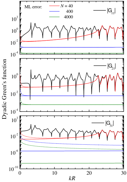
Figure 2: Elements $\mathcal{G}_{11}$, $\mathcal{G}_{21}$, and $\mathcal{G}_{31}$ of the TE block of the dyadic GF (black solid lines) of a homogeneous sphere in vacuum and the absolute error for the 2nd (dashed lines) and 4th (solid lines) ML representations, given by Eqs. (75) and (104), respectively, for the number of RSs $N$ in the ML series as given. Results are shown as function of the real wave number $k$, for a magnetic sphere in vacuum, having $\varepsilon=1$, $\mu=8$, and radius $R$. The coordinates of the GF are fixed at $r=0.5R$ and $r^{\prime}=0.6R$.

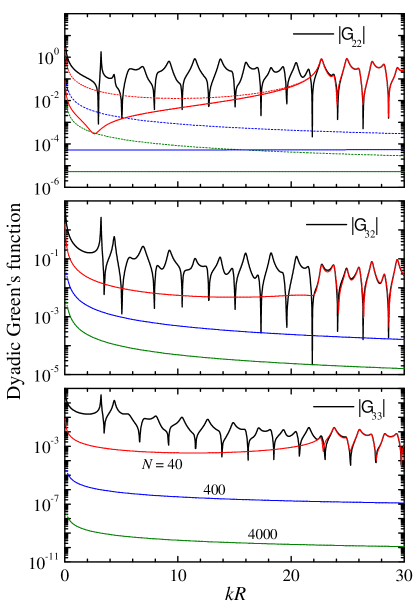
Figure 3: As Fig. 2 but for elements $\mathcal{G}_{22}$, $\mathcal{G}_{32}$, and $\mathcal{G}_{33}$.

V Numerical results

In this section, we provide a few illustrations of the most important results obtained in this work. More illustrations of these results and application of the RSE to different systems, analyzing in particular the efficiency of the versions introduced, will be presented elsewhere. Since the main focus of this paper is a proper elimination of static modes from the RSE, we concentrate below on the ML representations and the version of the RSE not containing static modes.

V.1 Convergence of ML representations

Two different ML series introduced above, namely the 2nd and the 4th ML representations, which do not contain static-mode contributions are given, respectively, by Eqs. (75) and (104). These equations describe the TE block of the GF which can be equally used for TM polarization by swapping $\varepsilon\leftrightarrow\mu$, as discussed in detail at the beginning of Sec. III. In particular, element $\mathcal{G}_{11}$ of the TE block is responsible for the electric field in TE polarization, while elements $\mathcal{G}_{22}$, $\mathcal{G}_{23}$, $\mathcal{G}_{32}$, and $\mathcal{G}_{33}$ effectively describe the electric field in TM polarization. To address the TM polarization of a dielectric sphere with $\varepsilon=8$ and $\mu=1$ taken for illustration, we therefore consider instead the TE block of the dyadic GF for a magnetic sphere with $\varepsilon=1$ and $\mu=8$.

Figures 2 and 3 show six elements of the TE block of the dyadic GF as a function of the real wave number $k$, for fixed $r=0.5R$ and $r^{\prime}=0.6R$. Three other elements, $\mathcal{G}_{12}$, $\mathcal{G}_{13}$, and $\mathcal{G}_{23}$, which are not shown, are quite similar to, respectively, $\mathcal{G}_{21}$, $\mathcal{G}_{31}$, and $\mathcal{G}_{32}$. The exact dyadic GF used for these plots is given by Eq. (47) with the left and right vector functions, $\mathbfcal{F}_{L}(r)$ and $\mathbfcal{F}_{R}(r)$, having the explicit analytic form provided in Eqs. (91) and (95), respectively. The exact GF is then compared with two ML representations, Eqs. (75) and (104), with the absolute difference shown in Figs. 2 and 3 for both representations, for different numbers $N$ of RSs included in the expansion, in order to see how the ML series converge to the exact values.

It is clear that the first three elements of the Green’s dyadic, illustrated in Fig. 2, are not diverging at $k=0$, in agreement with the analysis provided in Sec. III. Furthermore, element $\mathcal{G}_{11}$ vanishes at $k=0$, in accordance with Eq. (72). However, the 2nd ML representation Eq. (75) demonstrates some footprints of the $1/k$ pole in these elements. This feature comes from the expansion of a $\delta$ function into the RSs, which is included in this ML series. The $\delta$ function contributes with a pre-factor $1/k$ [see Eq. (75)], explaining the observed $1/k$ dependence of the error. The 4th ML representation Eq. (104) instead does not show any $1/k$ features and converges to the exact solution as $1/N$ for elements $\mathcal{G}_{11}$ and $\mathcal{G}_{21}$, and as $1/N^{3}$ for element $\mathcal{G}_{31}$, much quicker than the 2nd one.

We further compare in Fig. 3 the two ML series, Eqs. (75) and (104), for elements $\mathcal{G}_{22}$, $\mathcal{G}_{32}$, and $\mathcal{G}_{33}$ of the Green’s dyadic. Physically, these components contain a $k=0$ pole contribution due to the spatial inhomogeneity of the system, which is clearly seen in Fig. 3 as $1/k$ divergence. Note that this is additional to the longitudinal $\delta$-like singularity of the Green’s dyadic of the homogeneous space LevineCPAM50 , which should not be seen at $r\neq r^{\prime}$. Here, the difference between the two representations is only in the $\mathcal{G}_{22}$ component, which is again due to the fact that the 2nd ML representation Eq. (75) contains an expansion of a $\delta$ function contributing with a pre-factor $1/k$. This additional divergent contribution, making the series representation inefficient, is entirely eliminated in the 4th ML representation Eq. (104), as it is clear from the top panel of Fig. 3. As discussed in detail in Sec. III.5 above, this is the most significant improvement of the ML series implemented in the 3rd and also in the 4th ML representations, which results in a quickly convergent RSE, as demonstrated in Sec. V.2 below. The ML series converge as $1/N$ for $\mathcal{G}_{22}$ and $\mathcal{G}_{32}$ components and as $1/N^{3}$ for $\mathcal{G}_{33}$.

V.2 RSE for a shell perturbation of a homogeneous sphere

Consider a general spherical shell perturbation of the generalized permittivity Eq. (81) in the following form:

$$\Delta\hat{\mathcal{P}}(r)=\Theta(R_{2}-r)\Theta(r-R_{1})\left[\Delta\varepsilon\hat{\mathbf{1}}_{1}+\Delta\mu(\hat{\mathbf{1}}_{2}+\hat{\mathbf{1}}_{3})\right]\,,$$

where $R_{1}<R_{2}\leqslant R$. This includes as special cases:(i) a homogeneous perturbation of the permittivity and permeability over the full volume of the sphere ($R_{1}=0$, $R_{2}=R$), which we call strength perturbation; and(ii) reducing the radius of the sphere without changing its permittivity and permeability ($R_{1}>0$, $R_{2}=R$,$\Delta\varepsilon=1-\varepsilon$, $\Delta\mu=1-\mu$), which is size perturbation.

For a shell perturbation within a region $R_{1}<r<R_{2}$, the matrix elements between RSs $\mathbfcal{F}_{n}(r)$ and $\mathbfcal{F}_{m}(r)$ of TE polarization, contributing to the RSE equation (85) are given by

$$V_{nm} = \Delta\varepsilon\int_{R_{1}}^{R_{2}}\mathcal{E}_{n}(r)\mathcal{E}_{m}(r)dr+\Delta\mu\int_{R_{1}}^{R_{2}}\mathcal{K}_{n}(r)\mathcal{K}_{m}(r)dr$$ (105)

$$+\frac{\mu\Delta\mu}{\mu+\Delta\mu}\int_{R_{1}}^{R_{2}}\mathcal{N}_{n}(r)\mathcal{N}_{m}(r)dr\,.$$

Other elements, between RS wave functions $\mathbfcal{F}_{n}(r)$ and functions ${\boldsymbol{\Psi}}_{j}(r)$ representing the $k=0$ pole of the dyadic GF, or between function ${\boldsymbol{\Psi}}_{j}(r)$ and ${\boldsymbol{\Psi}}_{j^{\prime}}(r)$ [see Eqs. (79) and (104)], have a similar form, and all necessary integrals contributing to the matrix elements are provided in Appendix C.

As noted above, we illustrate in this paper only the versions of the RSE with static modes eliminated.

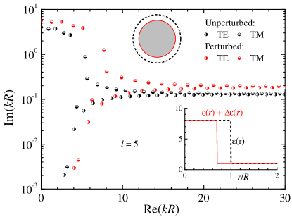
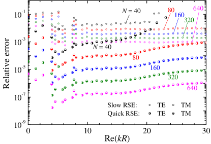
Figure 4: The RSE used for a size perturbation. Top: Wave numbers of TE and TM RSs for the unperturbed (black circles) and perturbed system (red circles). The unperturbed (perturbed) system is a homogeneous dielectric sphere in vacuum, with radius $R$ (0.7$R$), permittivity $\varepsilon=8$, and permeability $\mu=1$. The inset shows the profiles of the permittivity of the unperturbed and perturbed systems (black dashed and red solid lines, respectively). Bottom: Relative error of the TE an TM RS wave numbers, calculated by the RSE with static mode elimination. Results are shown for the slow RSE Eq. (24) and the quick RSE Eq. (85), corresponding, respectively to the 2nd and 4th ML representations, for different basis sizes $N$ as given.

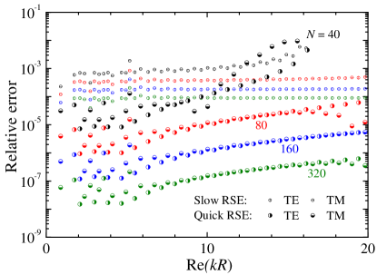
Figure 5: As Fig. 4 but for a strength perturbation of the sphere from $\varepsilon=8$ to $\varepsilon+\Delta\varepsilon=15$.

V.2.1 Size perturbation

For the size perturbation, we modify the optical system from a dielectric sphere of radius $R$ and permittivity $\varepsilon=8$ to the same-permittivity sphere of radius $0.7R$. We calculate both TE and TM modes of the smaller sphere using the slow and the quick versions of the RSE, both with static modes eliminated, and given by Eqs. (24) and (85), respectively. These versions correspond, respectively, to the 2nd and 4th ML representations, given by Eqs. (75) and (104), which we have illustrated in Sec. V.1 above, comparing with each other and with the analytic GF.

Figure 4 shows the unperturbed and perturbed RS wave numbers for both TE and TM polarizations and the relative error for the modes of the smaller sphere calculated via the slow and quick RSE, demonstrating the same level of efficiency for both polarizations. Comparing the errors for different basis sizes $N$, it becomes clear that the quick (slow) RSE converges to the exact solution with relative error decreasing with $N$ as $1/N^{3}$ ($1/N$). Note that for this perturbation, the slow RSE has been already demonstrated for TM polarization in Fig. 1 above. Also note that for TE polarization, the quick RSE is identical to the original RSE formulated in MuljarovEPL10 . The latter was shown to have a quick convergence to the exact solution in the TE polarization and is included as a special case in the generalized version of the RSE introduced in Sec. III.6 and illustrated in Figs. 4 and 5, which is a major fundamental result of this paper. This generalized version works equally well for both TE and TM polarizations, as demonstrated by Figs. 4 and 5, and is capable of treating, on the same level of efficiency, perturbations mixing TE and TM polarizations, as well as basis RSs with different spherical quantum numbers $l,m$.

V.2.2 Strength perturbation

We show for consistency the strength perturbation which is also very easy to verify, as this perturbation transforms an exactly solvable homogeneous sphere into another homogeneous sphere. Results are presented in Fig. 5, showing that the convergence of both versions of the RSE is very similar to that in Fig. 4 for the size perturbation. Interestingly, for the strength perturbation, the overall level of errors is an order of magnitude smaller than for the size perturbation, even though the permittivity of the sphere in the strength perturbation is increased by almost a factor of two, while for the size perturbation the volume of the sphere is reduced by 2/3.

VI Conclusions

We have derived an analytic form of the electromagnetic Green’s dyadic of an arbitrary spherically symmetric open optical system. Applying the formalism of vector spherical harmonics, the $6\times 6$ tensor of the dyadic Green’s function (GF) comprising the electric and magnetic field components on equal footing, is mapped onto an $(l,m)$-diagonal radially dependent tensor which further splits into two $3\times 3$ blocks separating transverse electric (TE) and transverse magnetic (TM) polarizations. In each polarization, the dyadic GF is expressed in terms of the so-called left and right solutions of a 2nd-order scalar differential equation determining its radial dependence. For a uniform distribution of the permittivity and permeability within a sphere, we have provided a fully explicit analytic solution for the dyadic GF, in terms of the spherical Bessel and Hankel functions.

We have studied analytically the pole structure of the dyadic GF, explicitly demonstrating for a general spherically symmetric system the link between the normalization of the resonant states (RSs) and the pole residues of the dyadic GF at the RS frequencies. Using the analytic solution derived for the dyadic GF, we have also unambiguously determined its static pole residue, separating the regular part from the singularity described by a $\delta$ function and expanding this residue into different sets of static modes, as well as into the RSs themselves. This analysis has resulted in developing three different spectral representations of the dyadic GF of an arbitrary spherically symmetric system, which are called Mittag-Leffler (ML) representations. One more ML representation has also been found for a homogeneous sphere.

Different ML representations of the dyadic GF in turn generate different versions of the resonant-state expansion (RSE). In this paper, we have formulated in total four different versions of the RSE, two of them having slow and the other two quick convergence. Namely, they converge to the exact solution with the relative error proportional, respectively, to $1/N$ and $1/N^{3}$, where $N$ is the basis size used in the RSE. A comparative analysis of the four ML representations obtained in this work allowed us to reveal the source of poor convergence of the slow versions of the RSE, including the original one: Any expansion of the spatial singularity of the dyadic GF (related to its static pole) into a set of smooth functions, such as static modes or RS wave functions, slows down enormously the convergence of the RSE. With a simple elimination of static modes as introduced at the beginning of this paper, the convergence of the RSE does not improve, remaining as slow as in the original version.

The paper presents a solution to this challenge, which is a proper removal of the singularity from the ML series for the dyadic GF. A detailed analysis of the static pole of the GF allowed us to work out its regularized ML representations, with $\delta$-function singularities separated from the series. This resulted in a new, quickly convergent version of the RSE, presented here in two variants – with and without using static modes. While we have derived in this paper three different sets of static modes, also illustrating a significant freedom in their choice, we have focused in this work on the static-mode elimination. The main advantage of the RSE without static modes is that it depends only on a single parameter – the number $N$ of the physical RSs of the basis system included, which is in turn determined by the truncation frequency in the complex plane.

We have illustrated the RSE with static-mode elimination on exactly solvable examples, used for verification and convergence study. These are perturbations of a homogeneous dielectric sphere in vacuum reducing its radius or uniformly changing its refractive index. Separating the static-pole singulary of the dyadic GF allowed us to accurately describe the effective charges induced by inhomogeneities of the permittivity and permeability, which manifest themselves in RS fields that are not divergence free. This is proven by demonstrating the same level of convergence of the RSE both with and without induced charges, realized in the selected examples, respectively, in TM and TE polarizations.

The developed generalization of the RSE, efficient in taking the induced charges into account, is the main fundamental result of this work. While illustrated here on spherical systems only, this generalized RSE is capable of treating, on the same level of efficiency, non-spherical perturbations mixing TE and TM polarizations and different spherical quantum numbers $(l,m)$, which will be the focus of follow-up publications. Furthermore, as the RSE always maintains the completeness, it offers a unique tool for finding numerically exactly the full dyadic GF of an arbitrary non-spherical open optical system. Presently, this aim is not achievable by any other means.

Appendix A Vector spherical harmonics: definitions, properties, and application

The VSHs are defined by Eq. (26) with $Y_{lm}(\Omega)$ being the scalar spherical harmonics which are given by the following real functions:

$$Y_{lm}(\Omega)=\sqrt{\frac{2l+1}{2}\frac{(l-|m|)!}{(l+|m|)!}}P^{|m|}_{l}(\cos\theta)\chi_{m}(\varphi)\,,$$ (106)

where $P^{m}_{l}(x)$ are the associated Legendre polynomials, and

$$\chi_{m}(\varphi)=\left\{\begin{array}[]{lll}\pi^{-1/2}\sin(m\varphi)&{\rm for}&m<0\\ (2\pi)^{-1/2}&{\rm for}&m=0\\ \pi^{-1/2}\cos(m\varphi)&{\rm for}&m>0\,.\end{array}\right.$$ (107)

The orthonormality condition for the VSHs has the form LobanovPRA18

$$\int\textbf{Y}_{ilm}(\Omega)\cdot\textbf{Y}_{i^{\prime}l^{\prime}m^{\prime}}(\Omega)d\Omega=\delta_{ii^{\prime}}\delta_{ll^{\prime}}\delta_{mm^{\prime}}\,,$$ (108)

where $d\Omega=\sin\theta d\theta d\varphi$. From the definition Eq. (26) and the orthogonality Eq. (108) follow useful properties of the VSHs:

$$\textbf{Y}_{2lm}(\Omega)\times\textbf{Y}_{1lm}(\Omega)\cdot{\bf e}_{r} = \textbf{Y}_{1lm}^{2}(\Omega)\,,$$

$$\textbf{Y}_{3lm}(\Omega)\times\textbf{Y}_{1lm}(\Omega)\cdot{\bf e}_{r} = 0\,$$ (109)

(here ${\bf e}_{r}=\textbf{r}/r$), which are helpful for deriving the RS normalization Eq. (63).

Substituting the expansions Eq. (28) of $\textbf{E}(\textbf{r})$ and $\textbf{H}(\textbf{r})$ into Eq. (5), we obtain for the first Maxwell’s equation

$$0 = k\varepsilon(r)\textbf{E}(\textbf{r})-\nabla\times i\textbf{H}(\textbf{r})$$

$$= k\varepsilon(r)\sum_{jlm}E_{jlm}(r)\textbf{Y}_{jlm}-\nabla\times\sum_{jlm}iH_{jlm}(r)\textbf{Y}_{jlm}$$

$$= \left.\sum_{lm}\right\{\left[k\varepsilon(r)E_{1lm}(r)-\frac{1}{r}\frac{d}{dr}riH_{2lm}(r)-\frac{\alpha_{l}}{r}iH_{3lm}(r)\right]$$

$$\times\textbf{Y}_{1lm}+\left[k\varepsilon(r)E_{2lm}(r)+\frac{1}{r}\frac{d}{dr}riH_{1lm}(r)\right]\textbf{Y}_{2lm}$$

$$\left.+\sum_{lm}\left[k\varepsilon(r)E_{3lm}(r)+\frac{\alpha_{l}}{r}iH_{1lm}(r)\right]\textbf{Y}_{3lm}\right\}\,,$$

using $\nabla\times f(r)\textbf{Y}_{jlm}=f(r)\nabla\times\textbf{Y}_{jlm}+\textbf{r}\times\textbf{Y}_{jlm}f^{\prime}(r)/r$ and results for $\nabla\times\textbf{Y}_{jlm}$ and $\textbf{r}\times\textbf{Y}_{jlm}$ provided in LobanovPRA18 . Deriving a similar expression for the second Maxwell’s equation and using the orthonormality of the VSHs, Eq. (5) transforms into

$$\left(\begin{array}[]{cccccc}k\varepsilon&0&0&0&-\frac{1}{r}\frac{d}{dr}r&\frac{\alpha_{l}}{r}\\ 0&k\varepsilon&0&\frac{1}{r}\frac{d}{dr}r&0&0\\ 0&0&k\varepsilon&\frac{\alpha_{l}}{r}&0&0\\ 0&-\frac{1}{r}\frac{d}{dr}r&\frac{\alpha_{l}}{r}&k\mu&0&0\\ \frac{1}{r}\frac{d}{dr}r&0&0&0&k\mu&0\\ \frac{\alpha_{l}}{r}&0&0&0&0&k\mu\end{array}\right)\left(\begin{array}[]{c}E_{1lm}\\ E_{2lm}\\ E_{3lm}\\ iH_{1lm}\\ iH_{2lm}\\ iH_{3lm}\end{array}\right)=0\,.$$ (110)

The matrix in Eq. (110) can be made block-diagonal, by simultaneous swapping of its columns and rows, so that the full $6\times 6$ problem for each ($l,m$) splits into two blocks, one for TE, the other for TM polarization.

Let us also express the gradient operator in the basis of the VSHs. For an arbitrary scalar field $f(\textbf{r})$, we obtain

$$\nabla f(\textbf{r}) = \nabla\sum_{lm}f_{lm}(r)Y_{lm}$$

$$= \sum_{lm}[f_{lm}(r)\nabla Y_{lm}+Y_{lm}\nabla f_{lm}(r)]$$

$$= \sum_{lm}\left[\textbf{Y}_{2lm}\frac{\alpha_{l}}{r}f_{lm}(r)+\textbf{Y}_{3lm}\frac{d}{dr}f_{lm}(r)\right],$$

using the definition of the VSHs, Eq. (26). Then, for fixed $l$ and $m$, the gradient operator is given by Eq. (51).

Appendix B Derivation of the spherically symmetric dyadic GF

In this Appendix, we derive Eqs. (41), (50), and (53), describing the analytic behaviour of the dyadic GF of a spherically symmetric open optical system and its residue at the static, $k=0$ pole.

First of all, it is straightforward to obtain Eq. (42), by excluding $\mathcal{G}_{21}$ and $\mathcal{G}_{31}$ from the simultaneous equations given by Eq. (39). We then find from the same equation that

$$\mathcal{G}_{21}(r,r^{\prime})=-\frac{1}{k\mu(r)}\frac{d}{dr}\mathcal{G}_{11}(r,r^{\prime})$$

and, using the reciprocity relation Eq. (40), obtain

$$\mathcal{G}_{12}(r,r^{\prime})=\mathcal{G}_{21}(r^{\prime},r)=-\frac{1}{k\mu(r^{\prime})}\frac{d}{dr^{\prime}}\mathcal{G}_{11}(r,r^{\prime})\,.$$

From the last equation and again, from Eq. (39), we then find

$$\!\!\!\!\!\!\!\!\!\!\!\mathcal{G}_{22}(r,r^{\prime}) = \frac{\delta(r-r^{\prime})}{k\mu(r)}-\frac{1}{k\mu(r)}\frac{d}{dr}\mathcal{G}_{11}(r,r^{\prime})$$ (111)

$$= \frac{\delta(r-r^{\prime})}{k\mu(r)}+\frac{1}{k^{2}\mu(r)\mu(r^{\prime})}\frac{d}{dr}\frac{d}{dr^{\prime}}\mathcal{G}_{11}(r,r^{\prime}).$$

Note that $\mathcal{G}_{22}$ is a regular component of the dyadic GF, and the $\delta$ function which appears explicitly in Eq. (111) is needed to exactly compensate on the same singularity of the second term in Eq. (111), which is due to the double differentiation. In fact, integrating Eq. (42), we find

$$\frac{1}{k\mu(r)}\frac{d}{dr}\mathcal{G}_{11}(r,r^{\prime})=f(r,r^{\prime})+\Theta(r-r^{\prime})\,,$$ (112)

where $f(r,r^{\prime})$ is a continuous regular function and $\Theta(x)$ is the Heaviside step function. Then

$$\frac{1}{k\mu(r)}\frac{d}{dr}\frac{d}{dr^{\prime}}\mathcal{G}_{11}(r,r^{\prime})=\frac{d}{dr^{\prime}}f(r,r^{\prime})-\delta(r-r^{\prime})\,,$$

demonstrating the above mentioned singularity.

We next evaluate from Eq. (39)

$$\mathcal{G}_{32}(r,r^{\prime}) = \mathcal{G}_{23}(r^{\prime},r)=-\frac{\alpha}{kr\mu(r)}\mathcal{G}_{12}(r,r^{\prime})$$

$$= \frac{\alpha}{k^{2}r\mu(r)\mu(r^{\prime})}\frac{d}{dr^{\prime}}\mathcal{G}_{11}(r,r^{\prime})$$

and

$$\mathcal{G}_{31}(r,r^{\prime})=\mathcal{G}_{13}(r^{\prime},r)=-\frac{\alpha}{kr\mu(r)}\mathcal{G}_{11}(r,r^{\prime})\,.$$ (113)

The last element of the GF may be evaluated by combining Eqs. (39) and (113):

$$\mathcal{G}_{33}(r,r^{\prime}) = \frac{\delta(r-r^{\prime})}{k\mu(r)}-\frac{\alpha}{kr\mu(r)}\mathcal{G}_{13}(r,r^{\prime})$$

$$= \frac{\delta(r-r^{\prime})}{k\mu(r)}+\frac{\alpha^{2}}{k^{2}r\mu(r)r^{\prime}\mu(r^{\prime})}\mathcal{G}_{11}(r,r^{\prime})\,.$$

Clearly this element is irregular as it contains a singular term which is not compensated by any derivative. Collecting all the elements of the dyadic GF derived above, we arrive at Eq. (41).

Looking at the elements $\mathcal{G}_{12}$, $\mathcal{G}_{21}$, $\mathcal{G}_{23}$, and $\mathcal{G}_{32}$, evaluated above, we see that all of them have discontinuities at $r=r^{\prime}$, as they are expressed in terms of the first derivative of $\mathcal{G}_{11}$, which is discontinuous at $r=r^{\prime}$, according to Eq. (112).

Now we derive in a similar way the two forms of the solution of Eq. (49), provided in Sec. III.2, which are Eqs. (50) and (53). Excluding $\mathcal{R}_{12}$ and $\mathcal{R}_{32}$ from Eq. (49), we obtain a differential equation for $\mathcal{R}_{22}$:

$$\left[-\frac{1}{\alpha^{2}}\frac{d}{dr}r^{2}\mu(r)\frac{d}{dr}+\mu(r)\right]\mathcal{R}_{22}(r,r^{\prime})=\delta(r-r^{\prime})$$

which becomes Eq. (52) after a substitution

$$\mathcal{R}_{22}(r,r^{\prime})=-\alpha^{2}g(r,r^{\prime})\,.$$ (114)

Other elements can be found straightforwardly from Eq. (49):

$$\mathcal{R}_{32}(r,r^{\prime})=\mathcal{R}_{23}(r^{\prime},r)=\frac{r}{\alpha}\frac{d}{dr}\mathcal{R}_{22}(r,r^{\prime})\,.$$

and

$$\mathcal{R}_{33}(r,r^{\prime})=\frac{r}{\alpha}\frac{d}{dr}\mathcal{R}_{23}(r,r^{\prime})=\frac{rr^{\prime}}{\alpha^{2}}\frac{d}{dr}\frac{d}{dr^{\prime}}\mathcal{R}_{22}(r,r^{\prime})\,.$$

Then, using the link Eq. (114), we obtain the solution Eq. (50).

On the other hand, one can use instead element $\mathcal{R}_{33}$ as a start point. Introducing its regular part $\mathcal{R}_{33}^{R}$,

$$\mathcal{R}_{33}(r,r^{\prime})=\mathcal{R}_{33}^{R}(r,r^{\prime})+\frac{\delta(r-r^{\prime})}{\mu(r)}\,,$$

we obtain from Eq. (49)

$$\mathcal{R}_{23}(r,r^{\prime})=\mathcal{R}_{32}(r,r^{\prime})=\frac{1}{\mu(r)}\frac{d}{dr}\frac{r\mu(r)}{\alpha}\mathcal{R}_{33}^{R}(r,r^{\prime})$$

and the following differential equation for $\mathcal{R}_{33}^{R}$:

$$\left[-\frac{d}{dr}\frac{1}{\mu(r)}\frac{d}{dr}\frac{r\mu(r)}{\alpha}+\frac{\alpha}{r}\right]\mathcal{R}_{33}^{R}(r,r^{\prime})=-\frac{\alpha}{r\mu(r)}{\delta(r-r^{\prime})}{}\,.$$

Element $\mathcal{R}_{22}$ can then be found, by noting that

$$\mathcal{R}_{12}(r,r^{\prime})=-\frac{r\mu(r)}{\alpha}\mathcal{R}_{32}(r,r^{\prime})\,,$$

so that, again, from Eq. (49) we obtain

$$\mathcal{R}_{22}(r,r^{\prime})=\frac{\delta(r-r^{\prime})}{\mu(r)}-\frac{1}{\mu(r)}\frac{d}{dr}\mathcal{R}_{12}(r,r^{\prime})$$

$$=\frac{\delta(r-r^{\prime})}{\mu(r)}+\frac{1}{\mu(r)\mu(r^{\prime})}\frac{d}{dr}\frac{d}{dr^{\prime}}\frac{r\mu(r)r^{\prime}\mu(r^{\prime})}{\alpha^{2}}\mathcal{R}_{33}^{R}(r,r^{\prime})\,.$$

Introducing a scalar GF $\tilde{g}(r,r^{\prime})$ such that

$$r\mu(r)r^{\prime}\mu(r^{\prime})\mathcal{R}_{33}^{R}(r,r^{\prime})=\alpha^{2}\tilde{g}(r,r^{\prime})\,,$$

we arrive at Eqs. (53) and (55).

Appendix C Homogeneous sphere in vacuum

C.0.1 Green’s function $\mathcal{G}_{11}$

The general form of the scalar GF $\mathcal{G}_{11}(r,r^{\prime})$ is given by Eq. (43). For a homogeneous sphere in vacuum, the wave equation (35) with the operator $\hat{L}$ given by Eq. (36) becomes

$$\left(\frac{d^{2}}{dr^{2}}-\frac{\alpha^{2}}{r^{2}}+n_{r}^{2}k^{2}\right)\mathcal{E}(r)=0 \ \ \ r\leqslant R\,,$$ (115)

$$\left(\frac{d^{2}}{dr^{2}}-\frac{\alpha^{2}}{r^{2}}+k^{2}\right)\mathcal{E}(r)=0 \ \ \ \ r>R\,,$$ (116)

which are both wave equations for a homogeneous space in 3D. Their solution can therefore be expressed in terms of spherical Bessel functions:

$$\mathcal{E}(r)=\left\{\begin{array}[]{ll}C_{1}J(n_{r}kr)+C_{2}H(n_{r}kr)&r\leqslant R\\ B_{1}J(kr)+B_{2}H(kr)&r>R\,,\end{array}\right.$$ (117)

see Sec. IV.1 for the definition of $J(z)$ and $H(z)$. Note that Eqs. (115) and (116) have to be solved together with the boundary conditions of continuity of $\mathcal{E}(r)$ and $\frac{1}{\mu(r)}\frac{d}{dr}\mathcal{E}(r)$, following from Eqs. (35) and (36). These boundary conditions are equivalent to Maxwell’s boundary conditions of the continuity of the tangent components of the electric and magnetic fields, as it is clear from Eqs. (34), (37), and (38). The coefficients in Eq. (117) are thus found from these boundary conditions and the additional “left” and “right” boundary conditions Eq. (45). The latter lead to $C_{2}=0$ in the left and $B_{1}=0$ in the right solution. Also, without loss of generality, we have chosen $C_{1}=1$ in the left and $C_{2}=1$ in the right solution. The left and right solutions $\mathcal{E}_{L(R)}(r)$ then take the form of Eq. (87), in which the coefficients are given by

$$C(k) = -\frac{\beta H(z)H^{\prime}(n_{r}z)-H^{\prime}(z)H(n_{r}z)}{\beta H(z)J^{\prime}(n_{r}z)-H^{\prime}(z)J(n_{r}z)}\,,$$ (118)

$$B_{1}(k) = \frac{J(n_{r}z)H^{\prime}(z)-\beta J^{\prime}(n_{r}z)H(z)}{J(z)H^{\prime}(z)-J^{\prime}(z)H(z)}\,,$$

$$B_{2}(k) = -\frac{J(n_{r}z)J^{\prime}(z)-\beta J^{\prime}(n_{r}z)J(z)}{J(z)H^{\prime}(z)-J^{\prime}(z)H(z)}\,,$$

$$B_{3}(k) = \beta\frac{J(n_{r}z)H^{\prime}(n_{r}z)-\beta J^{\prime}(n_{r}z)H(n_{r}z)}{J(n_{r}z)H^{\prime}(z)-\beta J^{\prime}(n_{r}z)H(z)}\,,$$

where $z=kR$, $n_{r}$ and $\beta$ are defined in Eq. (86), and the primes mean the derivatives of the functions with respect to their arguments.

Calculating the Wronskian Eq. (44), we obtain

$$W=\frac{n_{r}}{\mu}\left[J(x)H^{\prime}(x)-J^{\prime}(x)H(x)\right]=i\beta\,,$$ (119)

using Eq. (86) and the Wronskian of the spherical Bessel equation Abramowitz1964 :

$$J(x)H^{\prime}(x)-J^{\prime}(x)H(x)=i\,.$$ (120)

C.0.2 RS normalization

Let us first obtain Eq. (99) for the normalization constant $A_{n}$, using the definition Eq. (98). For this purpose, we Taylor expand the denominator $D(k)$ in the constant $C(k)$ given by Eq. (118), up to first order about the point $k=k_{n}$:

$$D(k) = \beta H(z)J^{\prime}(n_{r}z)-H^{\prime}(z)J(n_{r}z)$$ (121)

$$\approx \beta[H(z_{0})+H^{\prime}(z_{0})(z-z_{0})]$$

$$\times[J^{\prime}(n_{r}z_{0})+J^{\prime\prime}(n_{r}z_{0})n_{r}(z-z_{0})]$$

$$-[H^{\prime}(z_{0})+H^{\prime\prime}(z_{0})(z-z_{0})]$$

$$\times[J(n_{r}z_{0})+J^{\prime}(n_{r}z_{0})n_{r}(z-z_{0})]$$

$$= (k-k_{n})R\frac{H(z_{0})}{J(n_{r}z_{0})}\left\{J^{\prime 2}(n_{r}z_{0})\varepsilon\left(\frac{1}{\mu}-1\right)\right.$$

$$\left.+J^{2}(n_{r}z_{0})\left[\frac{\alpha^{2}}{z_{0}^{2}}\left(\frac{1}{\mu}-1\right)+1-\varepsilon\right]\right\}\,,$$

where $z=kR$ and $z_{0}=k_{n}R$. In doing so we have used the secular equation (96) and Bessel’s equation

$$F^{\prime\prime}(z)=(\alpha^{2}/z^{2}-1)F(z)\,,$$ (122)

valid for $F(z)=J(z)$ or $F(z)=H(z)$ [compare with Eqs. (115) and (116)]. The numerator in $C(k)$ is given by

$$N(k_{n}) = -\beta H(z_{0})H^{\prime}(n_{r}z_{0})+H^{\prime}(z_{0})H(n_{r}z_{0})$$ (123)

$$= -\beta\frac{H(z_{0})}{J(n_{r}z_{0})}$$

$$\times\left[J(n_{r}z_{0})H^{\prime}(n_{r}z_{0})-J^{\prime}(n_{r}z_{0})H^{\prime}(n_{r}z_{0})\right]$$

$$= -i\beta\frac{H(z_{0})}{J(n_{r}z_{0})}\,,$$

again using the Wronskian Eq. (120) and the secular equation (96). Substituting $D(k)$ and $N(k_{n})$ from Eqs. (121) and (123) into the definition Eq. (98) and taking the limit, we obtain the normalization constant Eq. (99).

The same result can be obtained from the general normalization Eq. (II.1), or its spherically symmetric version Eq. (63). The latter can be written as

$$1=I_{V}+I_{S}\,,$$ (124)

where the volume integral $I_{V}$, for a homogeneous sphere, transforms into

$$I_{V} = \int_{0}^{R}(\varepsilon\mathcal{E}_{1}^{2}+\mu\mathcal{H}_{2}^{2}+\mu\mathcal{H}_{3}^{2})dr$$ (125)

$$= \frac{\varepsilon A_{n}^{2}}{n_{r}k_{n}}\int_{0}^{n_{r}z_{0}}\left[J^{2}(x)(1+\alpha^{2}/x^{2})+J^{\prime 2}(x)\right]dx$$

$$= \varepsilon A_{n}^{2}R\left[J^{2}(x)(1-\alpha^{2}/x^{2})+J^{\prime 2}(x)\right]_{x=n_{r}z_{0}}$$

with $z_{0}=k_{n}R$, after integrating by parts and using Eq. (122) and the analytic integral Eq. (150) given below.

For the surface term $I_{S}$, which is evaluated at point $r=R_{+}$ outside the sphere, we need to consider the RS wave function outside the system, which is given by

$$\mathbfcal{F}_{n}(r)\equiv\left(\begin{array}[]{c}\mathcal{E}_{n}(r)\\ \mathcal{K}_{n}(r)\\ \mathcal{N}_{n}(r)\end{array}\right)=B_{n}\left(\begin{array}[]{c}H(y)\\ -H^{\prime}(y)\\ -\alpha H(y)/y\end{array}\right)\,,$$

similar to Eq. (97), with $y=k_{n}r$ ($r>R$) and

$$B_{n}=A_{n}J(n_{r}z_{0})/H(z_{0})\,.$$ (126)

We then obtain

$$\!\!\!\!\!\!I_{S} = \frac{R}{k_{n}}\left.\left(\mathcal{K}_{n}\frac{d\mathcal{E}_{n}}{dr}-\mathcal{E}_{n}\frac{d\mathcal{K}_{n}}{dr}\right)\right|_{r=R_{+}}$$ (127)

$$= B^{2}_{n}R[-H^{\prime 2}(z_{0})+H(z_{0})H^{\prime\prime}(z_{0})]$$

$$= B^{2}_{n}R[-H^{\prime 2}(z_{0})+H^{2}(z_{0})(\alpha^{2}/z^{2}_{0}-1)]$$

$$= A^{2}_{n}R\left[-\beta^{2}J^{\prime 2}(n_{r}z_{0})+J^{2}(n_{r}z_{0})(\alpha^{2}/z_{0}^{2}-1)\right]\!,\ \ \ \$$

using Eqs. (96) and (126). Substituting Eqs. (125) and (127) into Eq. (124) we obtain the same normalization constant Eq. (99).

C.0.3 Static pole of the dyadic GF

The static pole residue of the dyadic GF is given by two alternative forms Eqs. (50) and (53), in terms of the scalar GFs $g$ and $\tilde{g}$, respectively. Let us find these GFs for a homogeneous sphere in vacuum. The first one has the following form

$$g(r,r^{\prime})=\frac{f_{L}(r_{<})f_{R}(r_{>})}{\mathcal{W}}\,,$$

where $f_{L}(r)$ and $f_{R}(r)$ are solutions of the differential equation

$$\left(\frac{1}{r^{2}}\frac{d}{dr}r^{2}\frac{d}{dr}-\frac{\alpha^{2}}{r^{2}}\right)f_{L,R}(r)=0$$

satisfying, respectively, the left and right boundary conditions, $f_{L}(0)=f_{R}(\infty)=0$. Both solutions, $f_{L}(r)$ and $f_{R}(r)$, satisfy also the continuity conditions on the sphere surface of $f(r)$ and $\mu(r)f^{\prime}(r)$, where $f^{\prime}=df/dr$. Therefore they take the following explicit form:

$$\begin{array}[]{l}f_{L}(r)=\left\{\begin{array}[]{ll}(r/R)^{l}&\ r\leqslant R\\ \tilde{A}(r/R)^{l}+\tilde{B}(r/R)^{-l-1}&\ r>R\,,\end{array}\right.\vskip 3.0pt plus 1.0pt minus 1.0pt\\ f_{R}(r)=\left\{\begin{array}[]{ll}\tilde{C}(r/R)^{l}+\tilde{D}(r/R)^{-l-1}&r\leqslant R\\ (r/R)^{-l-1}&r>R\,,\end{array}\right.\end{array}$$

where

$$\tilde{A}=\mu\tilde{D}=\frac{\mu l+l+1}{2l+1}\,,\ \ \ \ \tilde{B}=-\frac{l}{l+1}\mu\tilde{C}=-\frac{(\mu-1)l}{2l+1}\,.$$ (128)

The Wronskian is given by

$$\mathcal{W}=\mu(r)r^{2}[f_{L}(r)f^{\prime}_{R}(r)-f^{\prime}_{L}(r)f_{R}(r)]=-(\mu l+l+1)R\,.$$

The other scalar GF has a similar form:

$$\tilde{g}(r,r^{\prime})=\frac{\tilde{f}_{L}(r_{<})\tilde{f}_{R}(r_{>})}{\tilde{\mathcal{W}}}\,,$$

where $\tilde{f}_{L}(r)$ and $\tilde{f}_{R}(r)$ are solutions of the differential equation

$$\left(\frac{d^{2}}{dr^{2}}-\frac{\alpha^{2}}{r^{2}}\right)\tilde{f}_{L,R}(r)=0$$

with $\tilde{f}_{L,R}(r)$ and $\frac{1}{\mu(r)}\tilde{f}^{\prime}_{L,R}(r)$ being continuous, in accordance with Eq. (55). They also satisfy the individual conditions $\tilde{f}_{L}(0)=\tilde{f}_{R}(\infty)=0$. Therefore, they take the following form:

$$\begin{array}[]{l}\tilde{f}_{L}(r)=\left\{\begin{array}[]{ll}(r/R)^{l+1}&\ r\leqslant R\\ \tilde{D}(r/R)^{l+1}+\tilde{C}(r/R)^{-l}&\ r>R\,,\end{array}\right.\vskip 3.0pt plus 1.0pt minus 1.0pt\\ \tilde{f}_{R}(r)=\left\{\begin{array}[]{ll}\tilde{B}(r/R)^{l+1}+\tilde{A}(r/R)^{-l}&r\leqslant R\\ (r/R)^{-l}&r>R\,,\end{array}\right.\end{array}$$

where the constants $\tilde{A}$, $\tilde{B}$, $\tilde{C}$, and $\tilde{D}$ are given by Eq. (128). The Wronskian takes the form

$$\tilde{\mathcal{W}}=\frac{\tilde{f}_{L}(r)\tilde{f}^{\prime}_{R}(r)-\tilde{f}^{\prime}_{L}(r)\tilde{f}_{R}(r)]}{\mu(r)}=-\frac{\mu l+l+1}{\mu R}\,.$$

The scalar GFs $g$ and $\tilde{g}$, the static pole residue, and the 4th ML representation following from it are then given by explicit expressions provided in Sec. IV.3.

C.0.4 Static-mode sets

Set 1. This set of static modes is generated by the scalar GF $g(r,r^{\prime})$. For LM modes, the static-mode potentials are given by

$$\psi_{\lambda}(r)=\frac{\phi_{\lambda}(r)}{\lambda}\,,$$ (129)

where $\phi_{\lambda}(r)$ are solutions of the differential equation (58) with $w(r)=\mu(r)r^{2}$, which for a homogeneous sphere simplifies to

$$\left(\frac{1}{r^{2}}\frac{d}{dr}r^{2}\frac{d}{dr}-\frac{\alpha^{2}}{r^{2}}+\lambda^{2}\Theta(R-r)\right)\phi_{\lambda}(r)=0\,.$$ (130)

The above equation has to be solved with the boundary conditions of continuity of $\phi_{\lambda}(r)$ and $\mu(r)\phi^{\prime}_{\lambda}(r)$. This results in wave functions

$$\phi_{\lambda}(r)={\lambda}{A_{\lambda}}\left\{\begin{array}[]{ll}j_{l}(\lambda r)&\ r\leqslant R\\ j_{l}(\lambda R)(r/R)^{-l-1}&\ r>R\end{array}\right.$$ (131)

and in a secular equation determining the eigenvalues $\lambda$:

$$\lambda\mu Rj_{l}^{\prime}(\lambda R)+(l+1)j_{l}(\lambda R)=0\,.$$ (132)

Using Eq. (131), the normalization condition, given by Eq. (61), reduces to

$$1=\mu\int_{0}^{R}\phi^{2}_{\lambda}(r)r^{2}dr=A_{\lambda}^{2}\frac{\mu}{\lambda}\int_{0}^{\lambda R}J^{2}(x)dx\,,$$ (133)

which determines the normalization constants $A_{\lambda}$. The last integral has the analytic form Eq. (150) given below. The wave functions $\psi_{\lambda}(r)$ defined in this way through Eq. (129) present the VC basis set introduced in LobanovPRA19 . In terms of this basis, the scalar GF $g(r,r^{\prime})$, contributing to the static mode pole of the dyadic GF via Eq. (50), is expressed as

$$g(r,r^{\prime})=-\sum_{\lambda}\psi_{\lambda}(r)\psi_{\lambda}(r^{\prime})\,,$$ (134)

using the expansion Eq. (62) and the link Eq. (129).

Set 2. Using the explicit expressions Eq. (100) for the scalar GFs $g$ and $\tilde{g}$ in the region within the sphere $(r\leqslant R)$, we find

$$g(r,r^{\prime})=\frac{\tilde{g}(r,r^{\prime})}{\mu^{2}rr^{\prime}}-\frac{1}{\mu R}\,\frac{\mu-1}{\mu l+l+1}\xi(r)\xi(r^{\prime})\,,$$ (135)

where $\xi(r)$ is defined by Eq. (101) [see also Eqs. (102) and (103)]. The GF $\tilde{g}$, satisfying Eq. (55), has a series representation given by the general Eq. (62), now having the form

$$\tilde{g}(r,r^{\prime})=-\sum_{\lambda}\frac{\tilde{\phi}_{\lambda}(r)\tilde{\phi}_{\lambda}(r^{\prime})}{\lambda^{2}}\,,$$

where $\lambda$ satisfies another secular equation provided below. The static-mode functions $\tilde{\phi}_{\lambda}(r)$ are solutions of the differential equation

$$\left(\frac{d^{2}}{dr^{2}}-\frac{\alpha^{2}}{r^{2}}+\lambda^{2}\Theta(R-r)\right)\tilde{\phi}_{\lambda}(r)=0\,,$$ (136)

which respect the boundary conditions of continuity of $\tilde{\phi}_{\lambda}(r)$ and $\frac{1}{\mu(r)}\tilde{\phi}^{\prime}_{\lambda}(r)$, following from Eq. (58) used for $w(r)=1/\mu(r)$ in the operator $\hat{\cal L}(r)$. They have the following explicit form

$$\tilde{\phi}_{\lambda}(r)={\mu}{A}_{\lambda}\left\{\begin{array}[]{ll}J(\lambda r)&\ r\leqslant R\\ J(\lambda R)(r/R)^{-l}&\ r>R\,,\end{array}\right.$$

where $\lambda$ is given by a new secular equation

$$\lambda Rj_{l}^{\prime}(\lambda R)+(\mu l+1)j_{l}(\lambda R)=0\,.$$ (137)

The normalization constants are again defined by the general equation (61),

$$1=\frac{1}{\mu}\int_{0}^{R}\tilde{\phi}^{2}_{\lambda}(r)dr={A}_{\lambda}^{2}\frac{\mu}{\lambda}\int_{0}^{\lambda R}J^{2}(x)dx\,,$$ (138)

which results in exactly the same analytic expressions for ${A}_{\lambda}$ as given by Eq. (133).

Within the sphere $(r\leqslant R)$, a series representation of $g(r,r^{\prime})$ contributing to the static pole via Eq. (50), in terms of the potentials ${\psi}_{\lambda}(r)$ is given by

$$g(r,r^{\prime})=-\sum_{\lambda}{\psi}_{\lambda}(r){\psi}_{\lambda}(r^{\prime})-{\psi}_{0}(r){\psi}_{0}(r^{\prime})$$ (139)

with

$${\psi}_{\lambda}(r)={{A}_{\lambda}}j_{l}(\lambda r)$$

having the same form as in Set 1. The last term in Eq. (139) is described in terms of

$${\psi}_{0}(r)=\sqrt{\frac{1}{\mu R}\,\frac{\mu-1}{\mu l+l+1}}\left(\frac{r}{R}\right)^{l}\,,$$

which can be interpreted as an additional static mode with $\lambda=0$.

Set 3. We consider here one more set of static modes, called volume-surface charge (VSC) basis which was also introduced in LobanovPRA19 . This set of modes corresponds to a rather extreme boundary condition which is that the wave function is vanishing everywhere outside the system. The differential equation for these static modes is similar to Eqs. (130) and (136):

$$\left(\frac{1}{r^{2}}\frac{d}{dr}r^{2}\frac{d}{dr}-\frac{\alpha^{2}}{r^{2}}+\lambda^{2}\right)\bar{\phi}_{\lambda}(r)=0\,,$$ (140)

this time lacking any Heaviside function. In fact, it needs to be solved only within a finite interval $0\leqslant r\leqslant R$ with the boundary condition $\bar{\phi}_{\lambda}(R)=0$, leading to the most simple secular equation

$$j_{l}(\lambda R)=0\,.$$ (141)

The wave functions of the static modes are given by

$$\psi_{\lambda}(r)=\frac{\bar{\phi}_{\lambda}(r)}{\sqrt{\mu}\lambda}={A}_{\lambda}j_{l}(\lambda r)\,,$$ (142)

and the normalization constants ${A}_{\lambda}$, again determined by Eq. (61), this time with $w(r)=r^{2}$, are thus taking the form

$$1=\int_{0}^{R}\bar{\phi}^{2}_{\lambda}(r)r^{2}dr={A}_{\lambda}^{2}\frac{\mu}{\lambda}\int_{0}^{\lambda R}J^{2}(x)dx\,,$$ (143)

identical to Eqs. (133) and (138).

In order to use this set of static modes, let us introduce a scalar GF $\bar{g}(r,r^{\prime})$ corresponding to the problem described by Eq. (140). It satisfies a differential equation

$$\left(\frac{1}{r^{2}}\frac{d}{dr}r^{2}\frac{d}{dr}-\frac{\alpha^{2}}{r^{2}}\right)\bar{g}(r,r^{\prime})=\frac{\delta(r-r^{\prime})}{r^{2}}$$ (144)

and vanishing boundary conditions, $\bar{g}(R,r^{\prime})=\bar{g}(r,R)=0$. Solving Eq. (144) with the help of the left and right functions,

$$\bar{g}(r,r^{\prime}) = \frac{\bar{f}_{L}(r_{<})\bar{f}_{R}(r_{>})}{\bar{W}}\,,$$

$$\bar{f}_{L}(r) = (r/R)^{l}\,,$$

$$\bar{f}_{R}(r) = -(r/R)^{l}+(r/R)^{-l-1}\,,$$

$$\bar{W} = r^{2}\left[\bar{f}_{L}(r)\bar{f}^{\prime}_{R}(r)-\bar{f}_{L}^{\prime}(r)\bar{f}_{R}(r)\right]=-(2l+1)R\,,$$

we find

$$\bar{g}(r,r^{\prime})=\frac{1}{(2l+1)R}\xi(r)\xi(r^{\prime})-\frac{1}{(2l+1)R}\xi(r_{<})\eta(r_{>})\,,$$ (145)

where functions $\xi(r)$ and $\eta(r)$ are defined by Eq. (101). On the other hand, $\bar{g}(r,r^{\prime})$ has the static-mode representation,

$$\bar{g}(r,r^{\prime})=-\sum_{\lambda}\frac{\bar{\phi}_{\lambda}(r)\bar{\phi}_{\lambda}(r^{\prime})}{\lambda^{2}}\,,$$ (146)

according to Eq. (62). Comparing Eqs. (145) and (100), and using the series Eq. (146) and the relation Eq. (142), we find

$$g(r,r^{\prime})=-\sum_{\lambda}{\psi}_{\lambda}(r){\psi}_{\lambda}(r^{\prime})-{\psi}_{0}(r){\psi}_{0}(r^{\prime})\,,$$ (147)

where

$${\psi}_{0}(r)=\sqrt{\frac{1}{R}\,\frac{1}{\mu l+l+1}}\left(\frac{r}{R}\right)^{l}\,.$$

Discussion. The static-mode sets considered above clearly demonstrate a flexibility of their choice for ML representations and the RSE. Comparing all three sets of static modes presented, we see that they provide alternative series representations of the scalar GF $g(r,r^{\prime})$. All three representation have the same form except that the series Eq. (134) for Set 1 is lacking the $\lambda=0$ term, as compared to Eqs. (139) and (147) which are identical. This term can be formally introduces for Set 1 as well, by defining a vanishing amplitude of the function $\psi_{0}(r)$ for this set. The normalization constants in $\psi_{0}(r)$ then take different analytic form among all three sets.

In all three sets of static modes, the basis wave functions (with $\lambda\neq 0$) have exactly the same form in terms of $\lambda$,

$$\psi_{\lambda}(r)={A}_{\lambda}j_{l}(\lambda r)\ \ (r\leqslant R)$$ (148)

with the normalization constants $A_{\lambda}$ given by the following explicit expressions LobanovPRA19 :

$$A_{\lambda}^{2}=\frac{2}{\mu\lambda^{2}R^{3}}\left[j^{2}_{l}(\lambda R)-j_{l-1}(\lambda R)j_{l+1}(\lambda R)\right]^{-1}\,.$$ (149)

The eigenvalues $\lambda$ are different for different static-mode sets and are determined by the secular equations (132), (137), and (141), following from different boundary conditions on the sphere surface, imposed for the static-mode wave functions. Consequently, the actual values of ${A}_{\lambda}$ and the actual wave functions $\psi_{\lambda}(r)$ are also different.

Using the relation Eq. (50) between the static pole of the dyadic GF and the scalar GF $g(r,r^{\prime})$, one can find from Eqs. (134), (139), and (147) the static-pole part of the 1st ML representation Eq. (68). In that representation, the vector functions $\mathbfcal{F}_{\lambda}(r)$ are defined by Eq. (69) with the scalar fields $\psi_{\lambda}(r)$ generated above for each set of modes. Note that when using Eq. (68) for Sets 2 and 3, the series should include a $\lambda=0$ term due to the additional effective static mode contributing to these sets, as discussed above. The 3rd ML representation Eq. (78) can be obtained from the above series for $g$, by using the relation between $g$ and $\mathcal{G}_{22}$ provided by Eq. (114). Finally, the effective $\lambda=0$ mode of Set 2 contributes to the last term of the 4th ML representation Eq. (104), in which all the physical static modes have been eliminated.

C.0.5 Matrix elements

Let us introduce for convenience the following analytic vector function

$$\mathbfcal{F}(k,r)\equiv\left(\begin{array}[]{c}\mathcal{E}(k,r)\\ \mathcal{K}(k,r)\\ \mathcal{N}(k,r)\end{array}\right)=\mathcal{A}(z)\left(\begin{array}[]{c}J(x)\\ -\beta J^{\prime}(x)\\ -\alpha\beta J(x)/x\end{array}\right)\,,$$

where $x=n_{r}kr$, $z=n_{r}kR$, and the normalization function $\mathcal{A}(z)$ is defined by Eq. (99). Clearly, $\mathbfcal{F}_{n}(r)=\mathbfcal{F}(k_{n},r)$ at the RS wave numbers $k_{n}$, see Eq. (97).

Looking at the ML representation Eq. (104), it is easy to see that only the integrals of the four products $\mathcal{E}(p,r)\mathcal{E}(q,r)$, $\mathcal{K}(p,r)\mathcal{K}(q,r)$, $\mathcal{N}(p,r)\mathcal{N}(q,r)$, and $\mathcal{K}(p,r)\mathcal{N}(q,r)$ contribute to all possible matrix elements for a spherical shell perturbation, three of them being already outlined in Eq. (105). This implies that the matrix elements can be expressed in terms of the following integrals of spherical Bessel functions:

$$I_{1}(p,q) = \int_{R_{1}}^{R_{2}}J(pr)J(qr)dr\,,$$

$$J_{1}(p,q) = \int_{R_{1}}^{R_{2}}J^{\prime}(pr)J^{\prime}(qr)dr\,,$$

$$J_{2}(p,q) = \int_{R_{1}}^{R_{2}}\frac{J(pr)}{pr}\frac{J(qr)}{qr}dr\,,$$

$$J_{3}(p,q) = \int_{R_{1}}^{R_{2}}J^{\prime}(pr)\frac{J(qr)}{qr}dr\,.$$

$I_{1}(p,q)$ is a well-known analytic integral, which is given by

$$I_{1}(p,q)=\left.\frac{qJ(pr)J^{\prime}(qr)-pJ^{\prime}(pr)J(qr)}{p^{2}-q^{2}}\right|_{R_{1}}^{R_{2}}$$

for $p\neq q$, and by

$$I_{1}(p,p)\!=\!\frac{1}{2p}\!\left[z\!\left\{\!J^{2}(z)\!\left(\!1\!-\!\frac{\alpha^{2}}{z^{2}}\right)\!+\!J^{\prime 2}(z)\!\right\}\!-\!J(z)J^{\prime}(z)\right]_{\!pR_{1}}^{\!pR_{2}}$$ (150)

for $p=q$. Integrals $J_{1}(p,q)$, $J_{2}(p,q)$, and $J_{3}(p,q)$, when considered separately, have to be evaluated numerically. Their combinations, however, produce another analytic integral:

$$I_{2}(p,q)=J_{1}(p,q)+\alpha^{2}J_{2}(p,q)\,,$$

which is given by

$$I_{2}(p,q)=\left.\frac{pJ(pr)J^{\prime}(qr)-qJ^{\prime}(pr)J(qr)}{p^{2}-q^{2}}\right|_{R_{1}}^{R_{2}}$$

for $p\neq q$, and by

$$I_{2}(p,p)\!=\!\frac{1}{2p}\!\left[z\!\left\{\!J^{2}(z)\!\left(\!1\!-\!\frac{\alpha^{2}}{z^{2}}\right)\!+\!J^{\prime 2}(z)\!\right\}\!+\!J(z)J^{\prime}(z)\right]_{\!pR_{1}}^{\!pR_{2}}$$

for $p=q$. Also, the following analytic integral may serve for verification of the numerics:

$$I_{3}(p,q)=J_{3}(p,q)+J_{3}(q,p)-J_{2}(p,q)=\left.\frac{J(pr)J(qr)}{pqr}\right|_{R_{1}}^{R_{2}}\,.$$

References

- (1) C. Tai, Dyadic Green’s functions in electromagnetic theory (Intext Educational Publishers, Scranton, 1971).
- (2) W. C. Chew, Waves and Fields in Inhomogeneous Media (IEEE Computer Society Press, New York, 1995).
- (3) H. T. Dung, L. Knöll, and D.-G. Welsch, Phys. Rev. A 62, 053804 (2000).
- (4) E. A. Muljarov and W. Langbein, Phys. Rev. B 94, 235438 (2016).
- (5) S. V. Lobanov, W. Langbein, and E. A. Muljarov, Phys. Rev. A 98, 033820 (2018).
- (6) T. Weiss and E. A. Muljarov, Phys. Rev. B 98, 085433 (2018).
- (7) H. Levine and J. Schwinger, Commun. Pure and Appl. Math. 3, 355 (1950).
- (8) C. Tai, Proceedings of the IEEE 61, 480 (1973).
- (9) R. E. Collin, Canadian Journal of Physics 51, 1135 (1973).
- (10) R. E. Collin, Electromagnetics 6, 183 (1986).
- (11) W. A. Johnson, A. Q. Howard, and D. G. Dudley, Radio Science 14, 961 (1979).
- (12) J. Wang, IEEE Transactions on Antennas and Propagation 30, 463 (1982).
- (13) P. Pathak, IEEE Transactions on Antennas and Propagation 31, 837 (1983).
- (14) G. Mie, Annalen der Physik 330, 377 (1908).
- (15) C. Bohren and D. R. Huffman, Absorption and Scattering of Light by Small Particles (Wiley Science Paperback Series, ADDRESS, 1998).
- (16) J. A. Stratton, Electro Magnetic Theory (McGraw-Hill Book Company, Inc., ADDRESS, 1941).
- (17) Le-Wei Li, Pang-Shyan Kooi, Mook-Seng Leong, and Tat-Soon Yee, IEEE Transactions on Microwave Theory and Techniques 42, 2302 (1994).
- (18) V. I. Okhmatovski and A. C. Cangellaris, IEEE Transactions on Antennas and Propagation 51, 3209 (2003).
- (19) Y. Kim, H. Chae, and S. Nam, Microwave and Optical Technology Letters 49, 1142 (2007).
- (20) A. Fallahi and B. Oswald, IEEE Transactions on Microwave Theory and Techniques 59, 1433 (2011).
- (21) C. Yeh, Phys. Rev. 131, 2350 (1963).
- (22) V. Daniele and M. Orefice, IEEE Transactions on Antennas and Propagation 32, 193 (1984).
- (23) R. M. More, Phys. Rev. A 4, 1782 (1971).
- (24) R. M. More and E. Gerjuoy, phys. Rev. A 7, 1288 (1973).
- (25) A. Muljarov, W. Langbein, and R. Zimmermann, Europhys Lett. 92, 50010 (2010).
- (26) M. B. Doost, W. Langbein, and E. A. Muljarov, Phys. Rev. A 87, 043827 (2013).
- (27) C. Sauvan, J. P. Hugonin, I. S. Maksymov, and P. Lalanne, Phys. Rev. Lett. 110, 237401 (2013).
- (28) Q. Bai et al., Opt. Express 21, 27371 (2013).
- (29) M. B. Doost, W. Langbein, and E. A. Muljarov, Phys. Rev. A 90, 013834 (2014).
- (30) M. Perrin, Opt. Express 24, 27137 (2016).
- (31) E. A. Muljarov and W. Langbein, Phys. Rev. B 93, 075417 (2016).
- (32) T. Weiss et al., Phys. Rev. Lett. 116, 237401 (2016).
- (33) T. Weiss et al., Phys. Rev. B 96, 045129 (2017).
- (34) S. V. Lobanov, G. Zoriniants, W. Langbein, and E. A. Muljarov, Phys. Rev. A 95, 053848 (2017).
- (35) E. A. Muljarov and T. Weiss, Opt. Lett. 43, 1978 (2018).
- (36) L. Zschiedrich et al., Phys. Rev. A 98, 043806 (2018).
- (37) W. Yan, R. Faggiani, and P. Lalanne, Phys. Rev. B 97, 205422 (2018).
- (38) P. Lalanne et al., Laser & Photonics Reviews 12, 1700113 (2018).
- (39) P. Lalanne et al., J. Opt. Soc. Am. A 36, 686 (2019).
- (40) H. S. Sehmi, W. Langbein, and E. A. Muljarov, Phys. Rev. B 101, 045304 (2020).
- (41) S. Neale and E. Muljarov, arXiv:1908.06916, Phys. Rev. B, accepted (2020).
- (42) P. M. Morse and H. Feshbach, Methods of theoretical physics, Vol. I and II (McGraw-Hill, New York, 1953).
- (43) S. V. Lobanov, W. Langbein, and E. A. Muljarov, Phys. Rev. A 100, 063811 (2019).
- (44) R. G. Barrera, G. A. Estevez, and J. Giraldo, European Journal of Physics 6, 287 (1985).
- (45) M. A. Kaliteevski et al., Phys. Rev. B 64, 115305 (2001).
- (46) H. Ajiki, T. Tsuji, K. Kawano, and K. Cho, Phys. Rev. B 66, 245322 (2002).
- (47) M. M. Glazov, E. L. Ivchenko, A. N. Poddubny, and G. Khitrova, Physics of the Solid State 53, 1753 (2011).
- (48) J. Wiersig, Phys. Rev. A 84, 063828 (2011).
- (49) G. B. Arfken and H. J. Weber, Mathematical Methods for Physicists, 5th edition (Academic Press, San Diego, 2001), p. 448.
- (50) M. Abramowitz and I. A. Stegun, Handbook of Mathematical Functions (Dover, New York, 1965).