Time-Response Functions of Fractional-Derivative
Rheological Models

Abstract

In view of the increasing attention to the time responses of complex fluids described by power-laws in association with the need to capture inertia effects that manifest in high-frequency microrheology, we compute the five basic time-response functions of in-series or in-parallel connections of two elementary fractional derivative elements known as the Scott-Blair (springpot) element. The order of fractional differentiation in each Scott-Blair element is allowed to exceed unity reaching values up to 2 and at this limit-case the Scott-Blair element becomes an inerter – a mechanical analogue of the electric capacitor that its output force is proportional only to the relative acceleration of its end-nodes. With this generalization, inertia effects may be captured beyond the traditional viscoelastic behavior. In addition to the relaxation moduli and the creep compliances, we compute closed form expressions of the memory functions, impulse fluidities (impulse response functions) and impulse strain-rate response functions of the generalized fractional derivative Maxwell fluid, the generalized fractional derivative Kelvin-Voigt element and their special cases that have been implemented in the literature. Central to these calculations is the fractional derivative of the Dirac delta function which makes possible the extraction of singularities embedded in the fractional derivatives of the two-parameter Mittag-Leffler function that emerges invariably in the time-response functions of fractional derivative rheological models.

1 Introduction

Phenomenological constitutive models containing differential operators of non-integer order (fractional - derivative models) have been proposed in mechanics, geosciences, electrical networks and biology over the last decades (Gemant 1936, 1938; Scott Blair 1944, 1947; Scott Blair et al. 1947; Scott Blair and Caffyn 1949; Caputo and Mainardi 1971; Rabotnov 1980; Bagley and Torvik 1983a, b; Koeller 1984; Koh and Kelly 1990; Friedrich 1991; Glöckle and Nonnenmacher 1991, 1994; Makris and Constantinou 1991; Schiessel et al. 1995; Makris 1997a; Gorenflo and Mainardi 1997; Challamel et al. 2013; Atanackovic et al. 2015; Westerlund and Ekstam 1994; Lorenzo and Hartley 2002; Suki et al. 1994; Puig-de-Morales-Marinkovic et al. 2007, and references reported therein). Given that fractional derivative operators are linear differential operators, the time-dependent behavior of mechanical, electrical or biological networks can be computed with frequency-domain techniques in association with the Fourier or Laplace transforms (Le Page 1961; Papoulis 1962; Bracewell 1965; Mainardi 2010).

There are several cases however, where the linear network that is described with a fractional derivative constitutive law is embedded in a wider system that behaves nonlinearly. As an example, seismic protection devices or rail pads which have been described with fractional derivative constitutive models (Koh and Kelly 1990; Makris and Constantinou 1991; Makris 1992; Zhu et al. 2015) belong to a structure or a vehicle-track system that may exhibit an overall nonlinear response. In this case the overall system response needs to be computed in the time-domain; therefore, a time-domain representation of the behavior of the individual components (devices) is needed. A time-domain representation is possible either by expressing the fractional derivatives with a time-series expansion, or by computing the basic time-response functions of the embedded linear networks and proceeding with an integral formulation to compute the overall system response.

When constitutive models with fractional-order derivatives are involved the numerical evaluation of the fractional derivative of a function is computationally demanding, partly because the fractional derivatives of the ”through” and ”across” variables of the linear network (stress, force, current = through variables and strain, displacement, voltage = across variables) need to be expressed via the Grünwald-Letnikov definition of the fractional derivative of order $q\in\mathbb{R}^{+}$ of a continuous function $f(t)$ (Oldham and Spanier 1974; Samko et al. 1974; Miller and Ross 1993; Podlubny 1998).

$$\frac{\mathrm{d}^{q}f(t)}{\mathrm{d}t^{q}}=D^{q}f(t_{j})=$$ (1)

$$\lim_{n\to\infty}\frac{\text{1}}{\Gamma(-q)}\left(\frac{t_{j}}{n}\right)^{-q}\sum\limits_{k=\text{0}}^{n-\text{1}}\frac{\Gamma(k-q)}{\Gamma(k+1)}f\left(t_{j}-k\frac{t_{j}}{n}\right)\text{,}\enskip q\in\mathbb{R}^{+}$$

where $\mathbb{R}^{+}$ is the set of positive real numbers.

The Grünwald-Letnikov definition given by Eq. (1) indicates that a large number of terms ($n\rightarrow\infty$) may be needed to meet satisfactory convergence and the computational effort may be intense (Makris 1992; Miller and Ross 1993). Accordingly, an integral formulation after deriving the basic time-response functions of the embedded linear networks that involve fractional differential operators emerge as an attractive alternative. Expressions of the relaxation modulus and the creep compliance of selective fractional derivative viscoelastic models have been presented by Smit and De Vries (1970); Koeller (1984); Friedrich (1991); Glöckle and Nonnenmacher (1991, 1994); Heymans and Bauwens (1994); Suki et al. (1994); Schiessel et al. (1995); Palade et al. (1996); Djordjević et al. (2003); Craiem and Magin (2010); Mainardi (2010); Mainardi and Spada (2011); Hristov (2019). The present work builds upon the aforementioned studies and constructs additional time-response functions such as the memory function, the impulse fluidity (impulse response function) and the impulse strain-rate response function of the generalized fractional Maxwell fluid and the generalized fractional Kelvin-Voigt element which are in series or in parallel connections of two elementary fractional-derivative elements known as the Scott-Blair (springpot) model (Scott Blair 1944, 1947). Special cases of these generalized fractional-derivative models are the spring – Scott-Blair in-series or parallel connections that have been used by Suki et al. (1994) to express the pressure–volume relation of the lung tissue viscoelastic behavior and subsequently used by Puig-de-Morales-Marinkovic et al. (2007) to model the viscoleastic behavior of human red blood cells. The springpot – dashpot in-series or parallel connections are rheological models have been used to capture the high-frequency behavior of semiflexible polymer networks (Gittes and MacKintosh 1998; Atakhorrami et al. 2008; Domínguez-García et al. 2014) or the behavior of viscoelastic dampers for the vibration and seismic isolation of structures (Makris 1992; Makris and Constantinou 1992; Makris and Deoskar 1996).

The memory function of the elementary Scott-Blair (springpot) element is central in this work, since it is the fractional derivative of the Dirac delta function which is merely the kernel appearing in the convolution of the Riemann-Liouville definition of the fractional derivative of a function. This finding shows that the fractional derivative of the Dirac delta function is finite everywhere other than at the singularity point and it is the inverse Fourier transform of $(\operatorname{i}\omega)^{q}$ with $q\in\mathbb{R}^{+}$. It emerges as a key function in the derivation of the time-response functions of generalized fractional derivative rheological models, since it makes possible the extraction of the singularities embedded in the fractional derivatives of the two-parameter Mittag-Leffler function.

2 Basic time-response functions of linear phenomenological models

This paper studies the integral representation of linear phenomenological constitutive models (linear networks) of the form

$$\left[\sum\limits_{m=\text{0}}^{M}a_{m}\frac{\mathrm{d}^{p_{m}}}{\mathrm{d}t^{p_{m}}}\right]\tau(t)=\left[\sum\limits_{n=\text{0}}^{N}b_{n}\frac{\mathrm{d}^{q_{n}}}{\mathrm{d}t^{q_{n}}}\right]\gamma(t)$$ (2)

where $\tau(t)$ and $\gamma(t)$ are the time-histories of the stress and the small-gradient strain, $a_{m}$ and $b_{n}$ are real-valued frequency-independent coefficients and the order of differentiation, $p_{m}$ and $q_{n}$ are real, positive non-integer numbers (usually rational fractions). A definition of the fractional derivative of order $q$ is given through the convolution integral

$$I^{q}\gamma(t)=\frac{\text{1}}{\Gamma(q)}\int_{c}^{t}\gamma(\xi)(t-\xi)^{q-\text{1}}\mathrm{d}\xi$$ (3)

where $\Gamma(q)$ is the Gamma function. When the lower limit, $c=\text{0}$, the integral given by Eq. (3) is often referred to as the Riemann-Liouville fractional integral (Oldham and Spanier 1974; Samko et al. 1974; Miller and Ross 1993; Podlubny 1998). The above integral converges only for $q>\text{0}$, or in the case where $q$ is a complex number, the integral converges for $\mathcal{R}(q)>\text{0}$. Nevertheless, by a proper analytic continuation across the line $\mathcal{R}(q)=\text{0}$, and provided that the function $f(t)$ in $n$ times differentiable, it can be shown that the integral given by Eq. (3) exists for $n-\mathbb{R}(q)>\text{0}$ (Riesz et al. 1949). In this case the generalized (fractional) derivative of order $q\in\mathbb{R}^{+}$ exists and is defined as

$$\frac{\mathrm{d}^{q}\gamma(t)}{\mathrm{d}t^{q}}=I^{-q}\gamma(t)=\frac{\text{1}}{\Gamma(-q)}\int_{\text{0}^{-}}^{t}\frac{\gamma(\xi)}{(t-\xi)^{q+\text{1}}}\mathrm{d}\xi\text{,}\enskip q\in\mathbb{R}^{+}$$ (4)

where $\mathbb{R}^{+}$ is the set of positive real numbers and the lower limit of integration, $\text{0}^{-}$, may engage an entire singular function at the time origin such as $\gamma(t)=\delta(t-\text{0})$ (Lighthill 1958; Mainardi 2010). Eq. (4) indicates that the fractional derivative of order $q$ of $\gamma(t)$ is essentially the convolution of $\gamma(t)$ with the kernel $\nicefrac{{t^{-q-\text{1}}}}{{\Gamma(-q)}}$ (Oldham and Spanier 1974; Samko et al. 1974; Miller and Ross 1993; Mainardi 2010). The Riemann-Liouville definition of the fractional derivative of order $q\in\mathbb{R}^{+}$ given by Eq. (4), where the lower limit of integration is zero, is central in this work since the strain and stress histories, $\gamma(t)$ and $\tau(t)$, are causal functions, being zero at negative times.

Linear viscoelastic materials, such as those described with Eq. (2), obey the so-called Boltzmann superposition principle – that the output response history can be obtained as the convolution of the input history after being convoluted with the corresponding time-response function. The basic time-response functions can be obtained either by imposing an impulse or a unit-step excitation on the constitutive model, or by inverting in the time-domain the corresponding frequency-response functions of the real-parameter constitutive model. Such techniques are well known in the literature of rheology (Ferry 1980; Bird et al. 1987; Tschoegl 1989), structural mechanics (Harris and Crede 1976; Veletsos and Verbic 1974; Makris 1997b) and automatic control (Bode 1945; Reid 1983; Triverio et al. 2007).

The linearity of Eq. (2) permits its transformation in the frequency domain

$$\tau(\omega)\left[\sum\limits_{m=\text{0}}^{M}a_{m}(\operatorname{i}\omega)^{p_{m}}\right]=\gamma(\omega)\left[\sum\limits_{n=\text{0}}^{N}b_{n}(\operatorname{i}\omega)^{q_{n}}\right]$$ (5)

where, $\operatorname{i}=\sqrt{-\text{1}}=$ imaginary unit, $\tau(\omega)=\int_{-\infty}^{\infty}\tau(t)e^{-\operatorname{i}\omega t}\mathrm{d}t$ and $\gamma(\omega)=\int_{-\infty}^{\infty}\gamma(t)e^{-\operatorname{i}\omega t}\mathrm{d}t$ are the Fourier transforms of the stress and strain histories and $(\operatorname{i}\omega)^{q}\gamma(\omega)$ is the Fourier Transform of the fractional derivative of order $q$ of the time function, $\gamma(t)$ (Oldham and Spanier 1974; Koh and Kelly 1990; Mainardi 2010; Samko et al. 1974; Miller and Ross 1993; Podlubny 1998)

$$\mathcal{F}\left\{\frac{\mathrm{d}^{q}\gamma(t)}{\mathrm{d}t^{q}}\right\}=\int_{-\infty}^{\infty}\frac{\mathrm{d}^{q}\gamma(t)}{\mathrm{d}t^{q}}e^{-\operatorname{i}\omega t}\mathrm{d}t=(\operatorname{i}\omega)^{q}\gamma(\omega)$$ (6)

Eq. (5) is expressed as

$$\tau(\omega)=\left[G_{\text{1}}(\omega)+\operatorname{i}G_{\text{2}}(\omega)\right]\gamma(\omega)$$ (7)

where $\mathcal{G}(\omega)=G_{\text{1}}(\omega)+\operatorname{i}G_{\text{2}}(\omega)]$ is the complex dynamic modulus of the constitutive model (Ferry 1980; Bird et al. 1987; Giesekus 1995).

$$\mathcal{G}(\omega)=G_{\text{1}}(\omega)+\operatorname{i}G_{\text{2}}(\omega)=\frac{\sum\limits_{n=\text{0}}^{N}b_{n}(\operatorname{i}\omega)^{q_{n}}}{\sum\limits_{m=\text{0}}^{M}a_{m}(\operatorname{i}\omega)^{p_{m}}}$$ (8)

and is a frequency-response function that relates a stress output to a strain input. The stress, $\tau(t)$, in Eq. (2) can be computed in the time domain with the convolution integral

$$\tau(t)=\int_{\text{0}}^{t}M(t-\xi)\gamma(\xi)\mathrm{d}\xi$$ (9)

where $M(t-\xi)$ is the memory function of the model (Bird et al. 1987; Veletsos and Verbic 1974; Makris 1997b), defined as the resulting stress at time $t$ due to an impulsive strain input at time $\xi$ ($\xi<t$), and is the inverse Fourier transform of the complex dynamic modulus

$$M(t)=\frac{\text{1}}{\text{2}\pi}\int_{-\infty}^{\infty}\mathcal{G}(\omega)e^{\operatorname{i}\omega t}\mathrm{d}\omega$$ (10)

The inverse of the complex dynamic modulus is the complex dynamic compliance Pipkin (1986); Giesekus (1995)

$$\mathcal{J}(\omega)=J_{\text{1}}(\omega)+\operatorname{i}J_{\text{2}}(\omega)=\frac{\text{1}}{\mathcal{G}(\omega)}=\frac{\sum\limits_{m=\text{0}}^{M}a_{m}(\operatorname{i}\omega)^{p_{m}}}{\sum\limits_{n=\text{0}}^{N}b_{n}(\operatorname{i}\omega)^{q_{n}}}$$ (11)

which is a frequency-response function that relates a strain output to a stress input. In structural mechanics the equivalent of the complex dynamic compliance is known as the dynamic flexibility, often expressed with $\mathcal{H}(\omega)$ (Clough and Penzien 1970). Accordingly, the strain history in Eq. (2) can be computed in the time domain via a convolution integral

$$\gamma(t)=\int_{\text{0}}^{t}\phi(t-\xi)\tau(\xi)\mathrm{d}\xi$$ (12)

where $\phi(t-\xi)$ is the impulse fluidity (Giesekus 1995), defined as the resulting strain history at time $t$ due to an impulsive stress input at time $\xi(t<\xi)$, and is the inverse Fourier transform of the dynamic compliance, $\mathcal{J}(\omega)$

$$\phi(t)=\frac{\text{1}}{\text{2}\pi}\int_{-\infty}^{\infty}\mathcal{J}(\omega)e^{\operatorname{i}\omega t}\mathrm{d}\omega$$ (13)

In structural mechanics, the equivalent of the impulse fluidity at the force–displacement level is known as the impulse response function, $h(t)$, which is the kernel appearing in the Duhamel integral (Clough and Penzien 1970; Veletsos and Verbic 1974; Makris 1997b). Expressions of the impulse fluidity of the Hookean solid, the Newtonian fluid, the Kelvin-Voigt solid and the Maxwell fluid have been presented by Giesekus (1995); whereas, for the three-parameter Poyinting-Thomson solid and the three- parameter Jeffreys fluid have been presented by Makris and Kampas (2009).

Table 1: Basic frequency-response functions and their corresponding causal time-response functions in linear viscoelasticity and linear network analysis. Because the time-response functions listed in the right column are zero at negative times, their Fourier transform shown in the left column is also a Laplace transform with variable $s=\operatorname{i}\omega$

Another useful frequency-response function of a linear constitutive model is the complex dynamic viscosity, $\eta(\omega)=\eta_{\text{1}}(\omega)+\operatorname{i}\eta_{\text{2}}(\omega)$, which relates a stress output to a strain-rate input

$$\tau(\omega)=\left[\eta_{\text{1}}(\omega)+\operatorname{i}\eta_{\text{2}}(\omega)\right]\accentset{\mbox{\large.}}{\gamma}(\omega)$$ (14)

where $\accentset{\mbox{\large.}}{\gamma}(\omega)=\operatorname{i}\omega\gamma(\omega)$ is the Fourier transform of the strain-rate history. In structural mechanics, the equivalent of the complex dynamic viscosity at the force-velocity level is known as the mechanical impedance, $\mathcal{Z}(\omega)=Z_{\text{1}}(\omega)+\operatorname{i}Z_{\text{2}}(\omega)$ (Harris and Crede 1976). The term impedance and its notation, $\mathcal{Z}(\omega)$, have also been used to express the pressure–volume-rate relation of the lung tissue viscoelastic behavior of human and selective animal lungs (Suki et al. 1994). For the linear viscoelastic model given by Eq. (2), the complex dynamic viscosity (impedance) of the model is

$$\eta(\omega)=\eta_{\text{1}}(\omega)+\operatorname{i}\eta_{\text{2}}(\omega)=\frac{\sum\limits_{n=\text{0}}^{N}b_{n}(\operatorname{i}\omega)^{q_{n}}}{\sum\limits_{m=\text{0}}^{M}a_{m}(\operatorname{i}\omega)^{p_{m}+\text{1}}}$$ (15)

The stress $\tau(t)$ in Eq. (2) can be computed in the time domain with an alternative convolution integral

$$\tau(t)=\int_{\text{0}}^{t}G(t-\xi)\frac{\mathrm{d}\gamma(\xi)}{\mathrm{d}\xi}\mathrm{d}\xi$$ (16)

where $G(t-\xi)$ is the relaxation modulus of the constitutive model defined as the resulting stress at the present time, $t$, due to a unit-step strain at time $\xi\text{ }(\xi<t)$ and is the inverse Fourier transform of the complex dynamic viscosity

$$G(t)=\frac{\text{1}}{\text{2}\pi}\int_{-\infty}^{\infty}\eta(\omega)e^{\operatorname{i}\omega t}\mathrm{d}\omega$$ (17)

Expressions for the relaxation modulus, $G(t)$, of the various simple viscoelastic models are well-known in the literature (Ferry 1980; Bird et al. 1987; Tschoegl 1989; Giesekus 1995). Expressions for the relaxation modulus of simple fractional derivative viscoelastic models have been presented by Smit and De Vries (1970); Koeller (1984); Friedrich (1991); Glöckle and Nonnenmacher (1991, 1994); Suki et al. (1994); Schiessel et al. (1995); Palade et al. (1996); Djordjević et al. (2003); Puig-de-Morales-Marinkovic et al. (2007); Mainardi (2010); Craiem and Magin (2010); Mainardi and Spada (2011); Jaishankar and McKinley (2013); Hristov (2019).

The inverse of the complex dynamic viscosity is the complex dynamic fluidity (Giesekus 1995)

$$\phi(\omega)=\phi_{\text{1}}(\omega)+\operatorname{i}\phi_{\text{2}}(\omega)=\frac{\text{1}}{\eta(\omega)}=\frac{\sum\limits_{m=\text{0}}^{M}a_{m}(\operatorname{i}\omega)^{p_{m}+\text{1}}}{\sum\limits_{n=\text{0}}^{N}b_{n}(\operatorname{i}\omega)^{q_{n}}}$$ (18)

which is a frequency-response function that relates a strain-rate output to a stress input. In structural mechanics the equivalent of the complex dynamic fluidity at the velocity-force level is known as the mechanical admittance or mobility (Harris and Crede 1976). The strain-rate history, $\accentset{\mbox{\large.}}{\gamma}(t)$, can be computed in the time domain via the convolution integral

$$\accentset{\mbox{\large.}}{\gamma}(t)=\frac{\mathrm{d}\gamma(t)}{\mathrm{d}t}=\int_{\text{0}}^{t}\psi(t-\xi)\tau(\xi)\mathrm{d}\xi$$ (19)

where $\psi(t-\xi)$ is the impulse strain-rate response function defined as the resulting strain-rate output at time $t$ due to an impulsive stress input at time $\xi(\xi<t)$ and is the inverse Fourier transform of the dynamic fluidity

$$\psi(t)=\frac{\text{1}}{\text{2}\pi}\int_{-\infty}^{\infty}\phi(\omega)e^{\operatorname{i}\omega t}\mathrm{d}\omega$$ (20)

Together with the relaxation modulus, $G(t-\xi)$ that appears as a kernel in Eq. (16), the other most popular time-response function in experimental stress analysis is the creep compliance, $J(t-\xi)$ (Ferry 1980; Pipkin 1986; Tschoegl 1989; Bird et al. 1987), that is defined as the resulting strain, $\gamma(t)$, at the present time $t$ due to a unit-step stress at time $\xi(\xi<t)$ and is the inverse Fourier transform of the complex creep function, $\mathcal{C}(\omega)$

$$J(t)=\frac{\text{1}}{\text{2}\pi}\int_{-\infty}^{\infty}\mathcal{C}(\omega)e^{\operatorname{i}\omega t}\mathrm{d}\omega$$ (21)

The complex creep function, $\mathcal{C}(\omega)$, is the ratio of the cyclic strain output $\gamma(\omega)$, over the cyclic stress-rate input $\accentset{\mbox{\large.}}{\tau}(\omega)$ (Mason et al. 1997; Mason 2000; Evans et al. 2009; Makris 2019).

$$\mathcal{C}(\omega)=\frac{\gamma(\omega)}{\accentset{\mbox{\large.}}{\tau}(\omega)}=\frac{\text{1}}{\operatorname{i}\omega}\mathcal{J}(\omega)$$ (22)

Under a unit-amplitude step-stress, $\tau(t)=U(t-\text{0})$ where $U(t-\text{0})$ is the Heaviside unit-step function, the strain history, $\gamma(t)$ is

$$\gamma(t)=\int_{\text{0}}^{t}J(t-\xi)\frac{\mathrm{d}\tau(\xi)}{\mathrm{d}\xi}\mathrm{d}\xi$$ (23)

All five time-response functions given by Eqs. (10), (13), (17) and (21) are causal time-response functions – that is they are zero at negative times. This means that their Fourier transform vanishes at negative times and it becomes one-sided. For instance, the complex dynamic viscosity, $\eta(\omega)$, that is the Fourier transform of the relaxation modulus, $G(t)$, is

$$\eta(\omega)=\int_{-\infty}^{\infty}G(t)e^{-\operatorname{i}\omega t}\mathrm{d}t=\int_{\text{0}}^{\infty}G(t)e^{-\operatorname{i}\omega t}\mathrm{d}t$$ (24)

The one-sided integral on the right-hand side of Eq. (24) that results from the causality of the time-response function, ($G(t)=\text{0}$ when $t<\text{0}$), is essentially the Laplace transform of the time-response function (Le Page 1961)

$$\eta(s)=\mathcal{L}\left\{G(t)\right\}=\int_{\text{0}}^{\infty}G(t)e^{-st}\mathrm{d}t$$ (25)

where $s=\operatorname{i}\omega$ is the Laplace variable and $\mathcal{L}$ indicates the Laplace transform operator. Accordingly, the frequency-response functions given by Eqs. (8), (11), (15), (18) and (22) are Laplace pairs with their corresponding time-response functions given by Eqs. (10), (13), (17) and (21), which are summarized in Table 1 when a strain input, strain-rate input, stress input or stress-rate input is imposed.

3 The fractional derivative of the Dirac delta function

Following the observations by Nutting (1921), that the stress response of several fluid-like materials to a step-strain decays following a power law $(\tau(t)=G(t)\sim t^{-q}$ with $\text{0}<q<\text{1})$ and the early work of Gemant (1936, 1938) on fractional differentials; Scott Blair (1944, 1947) pioneered the introduction of fractional calculus in viscoelasticity. With analogy to the Hookean spring, in which the stress is proportional to the zero-th derivative of the strain and the Newtonian dashpot, in which the stress is proportional to the first derivative of the strain, Scott Blair (1944, 1947); Scott Blair et al. (1947); Scott Blair and Caffyn (1949) proposed the springpot element – that is an element in-between a spring and a dashpot with constitutive law

$$\tau(t)=K_{q}\frac{\mathrm{d}^{q}\gamma(t)}{\mathrm{d}t^{q}}$$ (26)

where $q$ is a positive real number, 0 $\leq q\leq$ 1, $K_{q}$ is a phenomenological material parameter with units [M][L]${}^{-\text{1}}$[T]${}^{q-\text{2}}$ (say Pa-sec^q) and $\nicefrac{{\mathrm{d}^{q}\gamma(t)}}{{\mathrm{d}t^{q}}}$ is the fractional derivative of the strain-history defined by Eq. (4).

For the elastic Hookean spring with elastic modulus, $G$, its memory function as defined by Eq. (10) is $M(t)=G\delta(t-\text{0})$ – that is the zero-order derivative of the Dirac delta function; whereas, for the Newtonian dashpot with viscosity, $\eta$, its memory function is $M(t)=\eta\,$$\frac{\mathrm{d}\delta(t-\text{0})}{\mathrm{d}t}$ – that is the first-order derivative of the Dirac delta function (Bird et al. 1987, see also Table 2). Since the springpot element defined by Eq. (26) with 0 $\leq q\leq$ 1 is a constitutive model that is in-between the Hookean spring and the Newtonian dashpot, physical continuity suggests that the memory function of the springpot model given by Eq. (26) shall be of the form of $M(t)=K_{q}\,$ $\frac{\mathrm{d}^{q}\delta(t-\text{0})}{\mathrm{d}t^{q}}$ – that is the fractional derivative of order $q$ of the Dirac delta function (Oldham and Spanier 1974; Podlubny 1998).

The fractional derivative of the Dirac delta function emerges directly from the property of the Dirac delta function (Lighthill 1958)

$$\int_{-\infty}^{\infty}\delta(t-\xi)f(t)\mathrm{d}t=f(\xi)$$ (27)

By following the Riemann-Liouville definition of the fractional derivative of a function given by the convolution appearing in Eq. (4), the fractional derivative of order $q\in\mathbb{R}^{+}$ of the Dirac delta function is

$$\frac{\mathrm{d}^{q}\delta(t-\xi)}{\mathrm{d}t^{q}}=\frac{\text{1}}{\Gamma(-q)}\int_{\text{0}^{-}}^{t}\frac{\delta(\tau-\xi)}{(t-\tau)^{\text{1}+q}}\mathrm{d}\tau\text{,}\enskip q\in\mathbb{R}^{+}$$ (28)

and by applying the property of the Dirac delta function given by Eq. (27); Eq. (28) gives

$$\frac{\mathrm{d}^{q}\delta(t-\xi)}{\mathrm{d}t^{q}}=\frac{\text{1}}{\Gamma(-q)}\frac{\text{1}}{(t-\xi)^{\text{1}+q}}\text{,}\enskip q\in\mathbb{R}^{+}$$ (29)

Eq. (29) offers the remarkable result that the fractional derivative of the Dirac delta function of any order $q\in\left\{\mathbb{R}^{+}-\mathbb{N}\right\}$ is finite everywhere other than at $t=\xi$; whereas, the Dirac delta function and its integer-order derivatives are infinite-valued, singular functions that are understood as a monopole, dipole and so on; and we can only interpret them through their mathematical properties as the one given by Eq. (27). Figure 1 plots the fractional derivative of the Dirac delta function at $\xi=\text{0}$

$$\frac{\mathrm{d}^{q}\delta(t-\text{0})}{\mathrm{d}t^{q}}=\frac{\text{1}}{\Gamma(-q)}\frac{\text{1}}{t^{\text{1}+q}}\enskip\enskip\text{with}\enskip q\in\mathbb{R}^{+}\text{,}\enskip t>\text{0}$$ (30)

The result of Eq. (30) is identical to the alternative definition of the $n^{\text{th}}$ $(n\in\mathbb{N}_{\text{0}})$ derivative of the Dirac delta function presented by Gel’fand and Shilov (1964) with a proper interpretation of the quotien $\frac{\text{1}}{t^{n+\text{1}}}$ as a limit at $t=\text{0}$.

$$\frac{\mathrm{d}^{n}\delta(t-\text{0})}{\mathrm{d}t^{n}}=\frac{\text{1}}{\Gamma(-n)}\frac{\text{1}}{t^{n+\text{1}}}\enskip\text{with}\enskip n\in\mathbb{N}_{\text{0}}$$ (31)

where $\mathbb{N}_{\text{0}}$ is the set of positive integers including zero

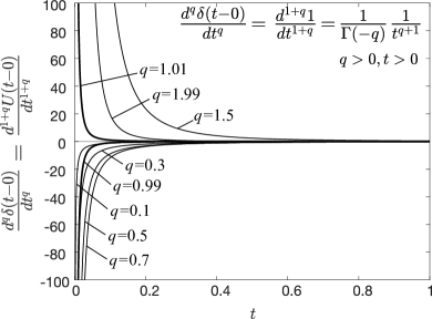
Figure 1: Plots of the fractional derivative of the Dirac delta function of order $q\in\left\{\mathbb{R}^{+}-\mathbb{N}\right\}$, which are the $\text{1}+q$ order derivative of the constant 1 for positive times. The functions are finite everywhere other than the time origin, $t=\text{0}$. Figure 1 shows that the fractional derivatives of the singular Dirac delta function and these of the constant unit at positive times are expressed with the same family of functions.

The result for the fractional derivative of the Dirac delta function given by Eq. (30) is also compared with the well known results in the literature for the fractional derivative of the constant unit function $f(t)=\text{1}$ (Oldham and Spanier 1974; Samko et al. 1974; Miller and Ross 1993; Podlubny 1998).

$$D^{r}\text{1}=\frac{t^{-r}}{\Gamma(\text{1}-r)}\text{,}\enskip r\in\mathbb{R}^{+}\enskip\text{and}\enskip t>\text{0}$$ (32)

For $r\in\mathbb{N}$, $D^{r}\text{1}=\text{0}$ due to the poles of the Gamma function at 0, -1, -2 and the classical results are recovered. Clearly, in Eq. (32) time needs to be positive ($t>\text{0}$); otherwise, the result of Eq. (32) would be a complex number when $r\in\left\{\mathbb{R}^{+}-\mathbb{N}\right\}$. Accordingly, a more formal expression of equation Eq. (32) within the context of generalized functions is

$$D^{r}U(t-\text{0})=\frac{\text{1}}{\Gamma(\text{1}-r)}\frac{\text{1}}{t^{r}}\text{,}\enskip r\in\mathbb{R}^{+}\text{,}\enskip t>\text{0}$$ (33)

where $U(t-\text{0})$ is the Heaviside unit-step function at the time origin (Lighthill 1958).

For the case where $r>\text{1}$, $\text{1}-r=-q$ with $q\in\mathbb{R}^{+}$; therefore $\text{1}+q=r>\text{1}$. Accordingly, for $r>\text{1}$, Eq. (33) can be expressed as

$$\frac{\mathrm{d}^{\text{1}+q}}{\mathrm{d}t^{\text{1}+q}}U(t-\text{0}) =\frac{\mathrm{d}^{q}}{\mathrm{d}t^{q}}\left[\frac{\mathrm{d}^{\text{1}}U(t-\text{0})}{\mathrm{d}t}\right]=$$ (34)

$$\frac{\mathrm{d}^{q}}{\mathrm{d}t^{q}}\delta(t-\text{0}) =\frac{\text{1}}{\Gamma(-q)}\frac{\text{1}}{t^{\text{1}+q}}\text{,}\enskip q\in\mathbb{R}^{+}\text{,}\enskip t>\text{0}$$

and the result of Eq. (30) is recovered. In Eq. (34) we used that $\delta(t-\text{0})=$ $\frac{\mathrm{d}^{\text{1}}U(t-\text{0})}{\mathrm{d}t}$ (Lighthill 1958).

4 Time-response functions of the Scott-Blair (springpot) element

The memory function, $M(t)$ appearing in Eq. (9), of the Scott-Blair $($springpot when 0 $\leq q\leq\text{1})$ element expressed by Eq. (26) results directly from the definition of the fractional derivative expressed with the Reimann-Liouville integral given by Eq. (4). Substitution of Eq. (4) into Eq. (26) gives

$$\tau(t)=\frac{K_{q}}{\Gamma(-q)}\int_{\text{0}}^{t}\frac{\gamma(\xi)}{(t-\xi)^{q+\text{1}}}\mathrm{d}\xi\text{,}\enskip q\in\mathbb{R}^{+}$$ (35)

By comparing Eq. (35) with Eq. (9), the memory function, $M(t)$, of the Scott-Blair (springpot when 0 $\leq q\leq$ 1) element is merely the kernel of the Riemann-Liouville convolution multiplied with the material parameter $K_{q}$

$$M(t)=\frac{K_{q}}{\Gamma(-q)}\frac{\text{1}}{t^{q+\text{1}}}=K_{q}\frac{\mathrm{d}^{q}\delta(t-\text{0})}{\mathrm{d}t^{q}}\text{,}\enskip q\in\mathbb{R}^{+}$$ (36)

where the right-hand side of Eq. (36) is from Eq. (30). Eq. (36) shows that the memory function of the springpot element is the fractional derivative of order $q\in\mathbb{R}^{+}$ of the Dirac delta function as was anticipated by using the argument of physical continuity given that the springpot element interpolates the Hookean spring and the Newtonian dashpot.

In this study we adopt the name “Scott-Blair element” rather than the more restrictive “springpot” element given that the fractional order of differentiation $q\in\mathbb{R}^{+}$ is allowed to take values larger than one. For instance when $\text{1}\leq q\leq\text{2}$ the Scott-Blair element represents an element that is in-between a dashpot and an inerter.

An “inerter” is a linear mechanical element where at the force-displacement level the output force is proportional only to the relative acceleration of its end-nodes (terminals) (Smith 2002; Papageorgiou and Smith 2005; Makris and Moghimi 2018) and complements the classical elastic spring and viscous dashpot. In a stress–current/strain-rate–voltage analogy, the inerter is the mechanical analogue of the electric capacitor and its constant of proportionality is the distributed inertance, $m_{R}$, with units of $\left[\text{M}\right]\left[\text{L}\right]^{-\text{1}}$ (say Pa-sec${}^{\text{2}}$). Studies in high-frequency microrheology (Mason and Weitz 1995; Indei et al. 2012; Domínguez-García et al. 2014) account for the distributed inertance $m_{R}=$ $\frac{m}{\text{6}\pi R}$, where $m$ and $R$ are the mass and radius of the particle (bead), respectively. When $q=\text{2}$, the memory function of the Scott-Blair element given by Eq. (36) gives

Figure 2: The Scott-Blair element with constitutive law $\tau(t)=K_{q}$$\nicefrac{{\mathrm{d}^{q}\gamma(t)}}{{\mathrm{d}t^{q}}}$ is an element in-between a spring ($K_{\text{0}}=G$) and a dashpot ($K_{\text{1}}=\eta$) when $\text{0}\leq q\leq\text{1}$ (springpot element) or an element in-between a dashpot ($K_{\text{1}}=\eta$) and an inerter ($K_{\text{2}}=m_{R}$) when $\text{1}\leq q\leq\text{2}$. In high-frequency microrheology the distributed inertance is $m_{R}=$ $\frac{m}{\text{6}\pi R}$ with units $\left[\text{M}\right]\left[\text{L}\right]^{-\text{1}}$, where $m$ and $R$ are the mass and radius of the particle (bead), respectively (Mason and Weitz 1995; Indei et al. 2012; Domínguez-García et al. 2014).

$$M(t)=\frac{K_{\text{2}}}{\Gamma(-\text{2})}\frac{\text{1}}{t^{\text{3}}}=m_{R}\frac{\mathrm{d}^{\text{2}}\delta(t-\text{0})}{\mathrm{d}t^{\text{2}}}$$ (37)

which is the memory function of the inerter (Makris 2017) and $K_{\text{2}}=m_{R}$ is its distributed inertance. The result offered by Eq. (37) is in agreement with the Gel’fand and Shilov (1964) alternative definition of the Dirac delta function and its integer-order derivatives offered by Eq. (31). Figure 2 shows schematically the Scott-Blair element that is in-between a spring ($K_{\text{0}}=G$) and a dashpot ($K_{\text{1}}=\eta$) when $\text{0}\leq q\leq\text{1}$ or in-between a dashpot ($K_{\text{1}}=\eta$) and an inerter ($K_{\text{2}}=m_{R}$) when $\text{1}\leq q\leq\text{2}$. Glöckle and Nonnenmacher (1991, 1993, 1994) studied the relaxation behavior of fractional derivative rheological models by implementing the Fox H-function and presented plots of the relaxation modulus of the spring – Scott-Blair element by allowing the fractional derivative of the Scott-Blair element to reach values up to 2 $(\text{0}\leq q\leq\text{2})$, a decade before Smith (2002) introduced the inerter and its direct equivalence to the electric capacitor. In this way Glöckle and Nonnenmacher (1994) have shown plots of the relaxation modulus of what we now call the inerto-elastic fluid (Makris 2017).

Eqs. (5) and (7) indicate that the complex dynamic modulus $\mathcal{G}(\omega)=G_{\text{1}}(\omega)+\operatorname{i}G_{\text{2}}(\omega)$ of the Scott-Blair element given bt Eq. (26) is

$$\mathcal{G}(\omega)=\frac{\tau(\omega)}{\gamma(\omega)}=K_{q}(\operatorname{i}\omega)^{q}$$ (38)

and its inverse Fourier transform is the memory function, $M(t)$, as indicated by Eq. (10). With the introduction of the fractional derivative of the Dirac delta function expressed by Eq. (29) or (36), the definition of the memory function given by Eq. (10) offers a new (to the best of our knowledge) and most useful result regarding the Fourier transform of the function $\mathcal{F}(\omega)=(\operatorname{i}\omega)^{q}$ with $q\in\mathbb{R}^{+}$

$$\mathcal{F}^{-\text{1}}(\operatorname{i}\omega)^{q}= \frac{\text{1}}{\text{2}\pi}\int_{-\infty}^{\infty}(\operatorname{i}\omega)^{q}e^{\operatorname{i}\omega t}\mathrm{d}\omega=$$ (39)

$$\frac{\mathrm{d}^{q}\delta(t-\text{0})}{\mathrm{d}t^{q}}=\frac{\text{1}}{\Gamma(-q)}\frac{\text{1}}{t^{q+\text{1}}}\text{,}\enskip q\in\mathbb{R}^{+}\text{,}\enskip t>\text{0}$$

In terms of the Laplace variable $s=\operatorname{i}\omega$ (see equivalence of Eqs. (24) and (25)), Eq. (39) gives that

$$\mathcal{L}^{-\text{1}}\left\{s^{q}\right\}=\frac{\mathrm{d}^{q}\delta(t-\text{0})}{\mathrm{d}t^{q}}=\frac{\text{1}}{\Gamma(-q)}\frac{\text{1}}{t^{q+\text{1}}}\text{,}\enskip q\in\mathbb{R}^{+}\text{,}\enskip t>\text{0}$$ (40)

where $\mathcal{L}^{-\text{1}}$ indicates the inverse Laplace transform operator (Le Page 1961; Mainardi 2010). While the right-hand side of Eq. (39) or (40) is non-zero only when $q\in\left\{\mathbb{R}^{+}-\mathbb{N}\right\}$ given the poles of the Gamma function when $q$ is zero or any positive integer; and assuming that we are not aware of the Gel’fand and Shilov (1964) definition of the Dirac delta function and its integer order derivatives given by Eq. (31); the validity of Eq. (39) can be confirmed by investigating its limiting cases. For instance, when, $q=\text{0}$, $(\operatorname{i}\omega)^{q}=\text{1}$; and Eq. (39) yields that $\frac{\text{1}}{\text{2}\pi}\int_{-\infty}^{\infty}e^{\operatorname{i}\omega t}\mathrm{d}\omega=\delta(t-\text{0})$; which is the correct result. When $q=\text{1}$, Eq. (39) yields that

$$\frac{\text{1}}{\text{2}\pi}\int_{-\infty}^{\infty}\operatorname{i}\omega e^{\operatorname{i}\omega t}\mathrm{d}\omega=\frac{\mathrm{d}\delta(t-\text{0})}{\mathrm{d}t}$$ (41)

Clearly, the function $\mathcal{F}(\omega)=\operatorname{i}\omega$ is not Fourier integrable in the classical sense, yet the result of Eq. (41) can be confirmed by evaluating the Fourier transform of $\frac{\mathrm{d}\delta(t-\text{0})}{\mathrm{d}t}$ together with the properties of the higher-order derivatives of the Dirac delta function (Lighthill 1958)

$$\int_{-\infty}^{\infty}\frac{\mathrm{d}^{n}\delta(t-\text{0})}{\mathrm{d}t^{n}}f(t)\mathrm{d}t=(-\text{1})^{n}\frac{\mathrm{d}^{n}f(\text{0})}{\mathrm{d}t^{n}}$$ (42)

By virtue of Eq. (42), the Fourier transform of $\frac{\mathrm{d}\delta(t-\text{0})}{\mathrm{d}t}$ is

$$\int_{-\infty}^{\infty}\frac{\mathrm{d}\delta(t-\text{0})}{\mathrm{d}t}e^{-\operatorname{i}\omega t}\mathrm{d}t=-(-\operatorname{i}\omega)e^{-\operatorname{i}\omega\text{0}}=\operatorname{i}\omega$$ (43)

therefore, the functions $\operatorname{i}\omega$ and $\frac{\mathrm{d}\delta(t-\text{0})}{\mathrm{d}t}$ are Fourier pairs, as indicated by Eq. (39).

More generally, for any $q=n\in\mathbb{N}$, Eq. (39) yields that

$$\frac{\text{1}}{\text{2}\pi}\int_{-\infty}^{\infty}(\operatorname{i}\omega)^{n}e^{\operatorname{i}\omega t}\mathrm{d}\omega=\frac{\mathrm{d}^{n}\delta(t-\text{0})}{\mathrm{d}t^{n}}$$ (44)

By virtue of Eq. (42), the Fourier transform of $\frac{\mathrm{d}^{n}\delta(t-\text{0})}{\mathrm{d}t^{n}}$ is

$$\int_{-\infty}^{\infty}\frac{\mathrm{d}^{n}\delta(t-\text{0})}{\mathrm{d}t^{n}}e^{\operatorname{i}\omega t}\mathrm{d}t=(-\text{1})^{n}(-\operatorname{i}\omega)^{n}=(\operatorname{i}\omega)^{n}$$ (45)

showing that the functions $(\operatorname{i}\omega)^{n}$ and $\frac{\mathrm{d}^{n}\delta(t-\text{0})}{\mathrm{d}t^{n}}$ are Fourier pairs, which is a special result (for $q\in\mathbb{N}_{\text{0}}$) of the more general result offered by Eq. (39). Consequently, fractional calculus and the memory function of the Scott-Blair element offer an alternative avenue to reach the Gel’fand and Shilov (1964) definition of the Dirac delta function and its integer order derivatives given by Eq. (31).

The complex dynamic compliance, $\mathcal{J}(\omega)$, of the Scott-Blair element as defined by Eq. (11) is the inverse of the complex dynamic modulus given by Eq. (38)

$$\mathcal{J}(\omega)=\frac{\gamma(\omega)}{\tau(\omega)}=\frac{\text{1}}{K_{q}}\frac{\text{1}}{(\operatorname{i}\omega)^{q}}$$ (46)

In terms of the Laplace variable, $s=\operatorname{i}\omega$, the impulse fluidity (impulse response function), $\phi(t)$, of the Scott-Blair element is given by

$$\phi(t)= \mathcal{L}^{-\text{1}}\left\{\mathcal{J}(s)\right\}=$$ (47)

$$\mathcal{L}^{-\text{1}}\left\{\frac{\text{1}}{K_{q}}\frac{\text{1}}{s^{q}}\right\}=\frac{\text{1}}{K_{q}}\frac{\text{1}}{\Gamma(q)}\frac{\text{1}}{t^{\text{1}-q}}U(t-\text{0})\text{,}\enskip q\in\mathbb{R}^{+}$$

The expression for the impulse fluidity (impulse response function) of the Scott-Blair element given by Eq. (47) has been also presented by Lorenzo and Hartley (2002). At the limit case where $q=\text{1}$, Eq. (47) gives $\phi(t)=$ $\frac{\text{1}}{K_{\text{1}}}\frac{\text{1}}{\Gamma(\text{1})}\frac{\text{1}}{t^{\text{0}}}$$U(t-\text{0})=$ $\frac{\text{1}}{K_{\text{1}}}$$U(t-\text{0})$, which is the impulse fluidity of the Newtonian fluid with viscosity $\eta=K_{\text{1}}$ (see Table 2). When $q=\text{2}$, Eq. (47) gives $\phi(t)=$ $\frac{\text{1}}{K_{\text{2}}}\frac{\text{1}}{\Gamma(\text{2})}$$tU(t-\text{0})=$ $\frac{\text{1}}{K_{\text{2}}}$$tU(t-\text{0})$, which is the impulse fluidity of the inerter with inertance $m_{R}=K_{\text{2}}$ (Makris 2017, 2018).

The complex dynamic viscosity (impedance), $\eta(\omega)$, of the Scott-Blair element as defined by Eq. (15) derives directly from Eq. (26) by using that $\accentset{\mbox{\large.}}{\gamma}(s)=s\gamma(s)$ with $s=\operatorname{i}\omega$. Accordingly, in the Laplace domain, the Scott-Blair element given by Eq. (26) is expressed as $\tau(s)=K_{q}s^{q-\text{1}}\accentset{\mbox{\large.}}{\gamma}(s)$ and therefore, the complex dynamic viscosity, $\eta(s)$, of the Scott-Blair element is

$$\eta(s)=K_{q}\frac{\text{1}}{s^{\text{1}-q}}\text{,}\enskip q\in\mathbb{R}^{+}$$ (48)

Table 2: Frequency-response functions and the corresponding causal time-response functions of the classical elementary rheological models and of the Scott-Blair element.

	Hookean Solid	Newtonian Fluid	Kelvin-Voigt Solid	Maxwell Fluid	Scott-Blair element
Constitutive Equation	$\tau(t)=G\gamma(t)$	$\tau(t)=\eta\frac{\mathrm{d}\gamma(t)}{\mathrm{d}t}$	$\tau(t)=G\gamma(t)+\eta\frac{\mathrm{d}\gamma(t)}{\mathrm{d}t}$	$\tau(t)+\lambda\frac{\mathrm{d}\tau(t)}{\mathrm{d}t}=\eta\frac{\mathrm{d}\gamma(t)}{\mathrm{d}t}$	$\tau(t)=K_{q}\frac{\mathrm{d}^{q}\gamma(t)}{\mathrm{d}t^{q}}$
Complex Dynamic Modulus $\mathcal{G}(\omega)=\frac{\tau(\omega)}{\gamma(\omega)}$	$G+\operatorname{i}\text{0}$	$\text{0}+\operatorname{i}\omega\eta$	$G+\operatorname{i}\omega\eta$	$\eta\left[\cfrac{\lambda\omega^{\text{2}}}{\text{1}+\lambda^{\text{2}}\omega^{\text{2}}}+\operatorname{i}\cfrac{\omega}{\text{1}+\lambda^{\text{2}}\omega^{\text{2}}}\right]$	$K_{q}(\operatorname{i}\omega)^{q}$
Complex Dynamic Viscosity $\mathcal{\eta}(\omega)=\frac{\tau(\omega)}{\accentset{\mbox{\large.}}{\gamma}(\omega)}$	$G\left[\pi\delta(\omega-\text{0})-\operatorname{i}\cfrac{\text{1}}{\omega}\right]$	$\eta+\operatorname{i}\text{0}$	$G\left[\lambda+\pi\delta(\omega-\text{0})-\operatorname{i}\cfrac{\text{1}}{\omega}\right]$	$\eta\left[\cfrac{\text{1}}{\text{1}+\lambda^{\text{2}}\omega^{\text{2}}}-\operatorname{i}\cfrac{\omega\lambda}{\text{1}+\lambda^{\text{2}}\omega^{\text{2}}}\right]$	$K_{q}\cfrac{\text{1}}{(\operatorname{i}\omega)^{\text{1}-q}}$
Complex Dynamic Compliance $\mathcal{J}(\omega)=\frac{\text{1}}{\mathcal{G}(\omega)}=\frac{\gamma(\omega)}{\tau(\omega)}$	$\cfrac{\text{1}}{G}+\operatorname{i}\text{0}$	$\cfrac{\text{1}}{\eta}\left[\pi\delta(\omega-\text{0})-\operatorname{i}\cfrac{\text{1}}{\omega}\right]$	$\cfrac{\text{1}}{G}\left[\cfrac{\text{1}}{\text{1}+\lambda^{\text{2}}\omega^{\text{2}}}-\operatorname{i}\cfrac{\omega\lambda}{\text{1}+\lambda^{\text{2}}\omega^{\text{2}}}\right]$	$\cfrac{\text{1}}{\eta}\left[\lambda+\pi\delta(\omega-\text{0})-\operatorname{i}\cfrac{\text{1}}{\omega}\right]$	$\cfrac{\text{1}}{K_{q}}\cfrac{\text{1}}{(\operatorname{i}\omega)^{q}}$
Complex Creep Function $\mathcal{C}(\omega)=\frac{\gamma(\omega)}{\accentset{\mbox{\large.}}{\tau}(\omega)}$	$\cfrac{\text{1}}{G}\left[\pi\delta(\omega-\text{0})-\operatorname{i}\cfrac{\text{1}}{\omega}\right]$	$\cfrac{\text{1}}{\eta}\left[-\cfrac{\text{1}}{\omega^{\text{2}}}+\operatorname{i}\pi\cfrac{\mathrm{d}\delta(\omega-\text{0})}{\mathrm{d}\omega}\right]$	$\frac{\text{1}}{G}\Big{[}\pi\delta(\omega-\text{0})-\operatorname{i}\frac{\text{1}}{\omega}$ $-\frac{\lambda}{\text{1}-\operatorname{i}\omega\lambda}\Big{]}$	$\frac{\text{1}}{G}\left[\pi\delta(\omega-\text{0})-\operatorname{i}\frac{\text{1}}{\omega}\right]+$ $+\frac{\text{1}}{\eta}\left[-\frac{\text{1}}{\omega^{\text{2}}}+\operatorname{i}\pi\frac{\mathrm{d}\delta(\omega-\text{0})}{\mathrm{d}\omega}\right]$	$\cfrac{\text{1}}{K_{q}}\cfrac{\text{1}}{(\operatorname{i}\omega)^{q+\text{1}}}$
Complex Dynamic Fluidity $\mathcal{\phi}(\omega)=\frac{\text{1}}{\eta(\omega)}=\frac{\accentset{\mbox{\large.}}{\gamma}(\omega)}{\tau(\omega)}$	$\text{0}+\operatorname{i}\omega\cfrac{\text{1}}{G}$	$\cfrac{\text{1}}{\eta}+\operatorname{i}\text{0}$	$\cfrac{\text{1}}{G}\left[\cfrac{\lambda\omega^{\text{2}}}{\text{1}+\lambda^{\text{2}}\omega^{\text{2}}}+\operatorname{i}\cfrac{\omega}{\text{1}+\lambda^{\text{2}}\omega^{\text{2}}}\right]$	$\cfrac{\text{1}}{\eta}\left[\text{1}+\operatorname{i}\lambda\omega\right]$	$\cfrac{\text{1}}{K_{q}}(\operatorname{i}\omega)^{\text{1}-q}$
Memory Function $M(t)$	$G\delta(t-\text{0})$	$\eta\cfrac{\mathrm{d}\delta(t-\text{0})}{\mathrm{d}t}$	$G\left[\delta(t-\text{0})+\lambda\frac{\mathrm{d}\delta(t-\text{0})}{\mathrm{d}t}\right]$	$G\left[\delta(t-\text{0})-\frac{\text{1}}{\lambda}e^{-t/\lambda}\right]$	$\cfrac{K_{q}}{\Gamma(-q)}\cfrac{\text{1}}{t^{q+\text{1}}}U(t-\text{0})$
Relaxation Modulus $G(t)$	$GU(t-\text{0})$	$\eta\delta(t-\text{0})$	$G\left[\lambda\delta(t-\text{0})+U(t-\text{0})\right]$	$Ge^{-t/\lambda}$	$\cfrac{K_{q}}{\Gamma(\text{1}-q)}\cfrac{\text{1}}{t^{q}}U(t-\text{0})$
Impulse Fluidity $\phi(t)$	$\cfrac{\text{1}}{G}\,\delta(t-\text{0})$	$\cfrac{\text{1}}{\eta}\,U(t-\text{0})$	$\cfrac{\text{1}}{\eta}\,e^{-t/\lambda}$	$\cfrac{\text{1}}{\eta}\left[\lambda\delta(t-\text{0})+U(t-\text{0})\right]$	$\cfrac{\text{1}}{K_{q}}\cfrac{\text{1}}{\Gamma(q)}\cfrac{\text{1}}{t^{\text{1}-q}}U(t-\text{0})$
Creep Compliance $J(t)$	$\cfrac{\text{1}}{G}\,U(t-\text{0})$	$\cfrac{\text{1}}{\eta}\,t\,U(t-\text{0})$	$\cfrac{\text{1}}{G}\,\left[U(t-\text{0})-e^{-t/\lambda}\right]$	$\cfrac{\text{1}}{G}\left(\text{1}+\cfrac{t}{\lambda}\right)U(t-\text{0})$	$\cfrac{\text{1}}{K_{q}}\cfrac{\text{1}}{\Gamma(q+\text{1})}t^{q}U(t-\text{0})$
Impulse Strain-rate Response Function $\psi(t)$	$\cfrac{\text{1}}{G}\cfrac{\mathrm{d}\delta(t-\text{0})}{\mathrm{d}t}$	$\cfrac{\text{1}}{\eta}\,\delta(t-\text{0})$	$\cfrac{\text{1}}{\eta}\left[\delta(t-\text{0})-\cfrac{\text{1}}{\lambda}e^{-t/\lambda}\right]$	$\cfrac{\text{1}}{\eta}\left[\delta(t-\text{0})+\lambda\frac{\mathrm{d}\delta(t-\text{0})}{\mathrm{d}t}\right]$	$\cfrac{\text{1}}{K_{q}}\cfrac{\text{1}}{\Gamma(-1+q)}\cfrac{\text{1}}{t^{\text{2}-q}}U(t-\text{0})$

For the springpot element $(\text{0}\leq q\leq\text{1})$ which is a special case of the Scott-Blair element $(q\in\mathbb{R}^{+})$ the quantity $\text{1}-q>\text{0}$, and the relaxation modulus, $G(t)$, of the springpot element is offered by the classical result available in Tables of Laplace transforms (Erdélyi 1954)

$$G(t)= \mathcal{L}^{-\text{1}}\left\{\eta(s)\right\}=\mathcal{L}^{-\text{1}}\left\{K_{q}\frac{\text{1}}{s^{\text{1}-q}}\right\}=$$ (49)

$$K_{q}\frac{\text{1}}{\Gamma(\text{1}-q)}\frac{\text{1}}{t^{q}}U(t-\text{0})\text{,}\enskip\text{0}<q<\text{1}$$

The result offered by Eq. (49) is well known to the literature (Smit and De Vries 1970; Koeller 1984; Friedrich 1991; Heymans and Bauwens 1994; Suki et al. 1994; Schiessel et al. 1995; Palade et al. 1996; Craiem and Magin 2010; Mainardi 2010). For the case where $q>\text{1}$ (say Scott-Blair element that is in between a dashpot and an inerter, $\text{1}\leq q\leq\text{2}$), the Laplace transform offered by the right-hand side of Eq. (49) does not exist in the classical sense and one has to use the result of Eq. (40). Accordingly for $q>\text{1}$, the complex dynamic viscosity of the Scott-Blair element is $\eta(s)=K_{q}s^{q-\text{1}}$ and Eq. (40) yields

$$G(t)= \mathcal{L}^{-\text{1}}\left\{K_{q}s^{q-\text{1}}\right\}=\frac{K_{q}}{\Gamma(-q+\text{1})}\frac{\text{1}}{t^{q-\text{1}+\text{1}}}U(t-\text{0})=$$ (50)

$$\frac{K_{q}}{\Gamma(\text{1}-q)}\frac{\text{1}}{t^{q}}U(t-\text{0})\text{,}\enskip q>\text{1}$$

Interestingly, the result offered by Eq. (50) for $q>1$ is identical to the classical result offered by Eq. (49) for $\text{0}\leq q<\text{1}$; therefore Eq. (49) is the expression of the relaxation modulus of the Scott-Blair element for any $q\in\mathbb{R}^{+}$. At the limit case where $q=\text{0}$, Eq. (49) gives $G(t)=K_{\text{0}}$$\frac{\text{1}}{\Gamma(\text{1})}\frac{\text{1}}{t^{\text{0}}}$$U(t-\text{0})=K_{\text{0}}U(t-\text{0})$ which is the relaxation modulus of the Hookean spring with elastic modulus $G=K_{\text{0}}$ (see Table 2). When $q=\text{1}$, Eq. (50) becomes the Dirac delta function, $\delta(t-\text{0})$, according to the definition given by Eq. (31) (Gel’fand and Shilov 1964); therefore, $G(t)=K_{\text{1}}\delta(t-\text{0})$ which is the relaxation modulus of the Newtonian dashpot with viscosity $\eta=K_{\text{1}}$ (see Table 2). When $q=\text{2}$, Eq. (50) yields $G(t)=$ $\frac{K_{\text{2}}}{\Gamma(-\text{1})}\frac{\text{1}}{t^{\text{2}}}$ $=K_{\text{2}}$$\frac{\mathrm{d}\delta(t-\text{0})}{\mathrm{d}t}$ which is the relaxation modulus of the inerter with inertance $m_{R}=K_{\text{2}}$ (Makris 2017, 2018).

The complex dynamic fluidity (admittance), $\phi(\omega)$, of the Scott-Blair element as defined by Eq. (18) is the inverse of its complex dynamic viscosity given by Eq. (48)

$$\phi(s)=\frac{\text{1}}{K_{q}}s^{\text{1}-q}\text{,}\enskip\text{0}<q<\text{1}$$ (51)

For the special case of the springpot element $(\text{0}\leq q\leq\text{1})$, $\text{1}-q\geq\text{0}$, the impulse strain-rate response function of the springpot element is offered with the help of Eq. (40)

$$\psi(t)= \mathcal{L}^{-\text{1}}\left\{\phi(s)\right\}=\mathcal{L}^{-\text{1}}\left\{\frac{\text{1}}{K_{q}}s^{\text{1}-q}\right\}=$$ (52)

$$\frac{\text{1}}{K_{q}}\frac{\text{1}}{\Gamma(-\text{1}+q)}\frac{\text{1}}{t^{\text{2}-q}}U(t-\text{0})\text{,}\enskip\text{0}\leq q\leq\text{1}$$

For the case where $q>\text{1}$ (say the Scott-Blair element that is in between a dashpot and an inerter: $\text{1}<q<\text{2}$) the complex dynamic fluidity of the Scott-Blair element is $\phi(s)=$ $\frac{\text{1}}{K_{q}}\frac{\text{1}}{s^{q-\text{1}}}$, and its inverse Laplace transform is offered from the classical result available in Tables of Laplace Transforms (Erdélyi 1954)

$$\psi(t)= \mathcal{L}^{-\text{1}}\left\{\phi(s)\right\}=\mathcal{L}^{-\text{1}}\left\{\frac{\text{1}}{K_{q}}\frac{\text{1}}{s^{q-\text{1}}}\right\}=$$ (53)

$$\frac{\text{1}}{K_{q}}\frac{\text{1}}{\Gamma(-\text{1}+q)}\frac{\text{1}}{t^{\text{2}-q}}U(t-\text{0})\text{,}\enskip q>\text{1}$$

The classical result offered by Eq. (53) for $q>\text{1}$ is identical to the result of Eq. (52) for $\text{0}<q<\text{1}$; therefore Eq. (53) is the expression of the impulse strain-rate response function of the Scott-Blair element for any $q\in\mathbb{R}^{+}$. For the limit cases where $q=\text{0}$ and $K_{q}=G$ or $q=\text{1}$ and $K_{q}=\eta$, Eq. (53) results by virtue of Eq. (31) that $\psi(t)=$ $\frac{\text{1}}{G}\frac{\mathrm{d}\delta(t-\text{0})}{\mathrm{d}t}$ or $\psi(t)=$ $\frac{\text{1}}{\eta}$$\delta(t-\text{0})$ which are respectively the impulse strain-rate response functions of the Hookean spring or the Newtonian dashpot, as shown in Table 2. For the limit case where $q=\text{2}$, Eq. (53) results, $\psi(t)=$ $\frac{\text{1}}{K_{\text{2}}}$$U(t-\text{0})$ which is the impulse strain-rate response function of the inerter with inertance $m_{R}=K_{\text{2}}$ (Makris 2017, 2018).

The complex creep function, $\mathcal{C}(\omega)$, of the Scott-Blair element as defined by Eq. (22) derives directly from equation (46) given that $\mathcal{C}(s)=$ $\frac{\mathcal{J}(s)}{s}$ with $s=\operatorname{i}\omega$. Accordingly, the complex creep function, $\mathcal{C}(s)$, of the Scott-Blair element is

$$\mathcal{C}(s)=\frac{\text{1}}{K_{q}}\frac{\text{1}}{s^{q+\text{1}}}\text{,}\enskip q\in\mathbb{R}^{+}$$ (54)

Given that $q+\text{1}>\text{0}$, the creep compliance of the Scott-Blair element is offered by the classical results available in Tables of Laplace transforms (Erdélyi 1954)

$$J(t)= \mathcal{L}^{-\text{1}}\left\{\mathcal{C}(s)\right\}=\mathcal{L}^{-\text{1}}\left\{\frac{\text{1}}{K_{q}}\frac{\text{1}}{s^{q+\text{1}}}\right\}=$$ (55)

$$\frac{\text{1}}{K_{q}}\frac{\text{1}}{\Gamma(q+\text{1})}t^{q}U(t-\text{0})\text{,}\enskip q\in\mathbb{R}^{+}$$

The expression given by Eq. (55) has been presented by Koeller (1984); Friedrich (1991); Heymans and Bauwens (1994); Schiessel et al. (1995). For the limit cases when $q=\text{0}$ and $K_{q}=G$ or $q=\text{1}$ and $K_{q}=\eta$, Eq. (55) results that $J(t)=$ $\frac{\text{1}}{G}$$U(t-\text{0})$ or $J(t)=$ $\frac{\text{1}}{\eta}$$tU(t-\text{0})$ which are respectively the creep compliances of the Hookean spring or the Newtonian dashpot shown in Table 2.

The five causal time-response functions of the Scott-Blair (springpot) element computed in this section (Eqs. (36), (47), (49), (52) and (55)) are summarized in Table 2 next to the known time-response function of the Hookean spring, the Newtonian dashpot, the Kelvin-Voigt solid and the Maxwell fluid (Harris and Crede 1976; Bird et al. 1987; Giesekus 1995; Makris 1997b) which are included to validate the limit-cases of the results derived for the generalized fractional derivative rheological models examined in this work.

Figure 3: The generalized fractional Maxwell fluid (left) and the generalized fractional Kelvin-Voigt element (right) with $p$, $q\in\mathbb{R}^{+}$.

5 Two-parameter fractional derivative rheological models

Upon we introduced the fractional derivative of the Dirac delta function and derived the causal time-response functions of the elementary Scott-Blair element expressed by Eq. (26); this study proceeds with the derivation of the time-response functions of the two-parameter generalized fractional Maxwell fluid and generalized fractional Kelvin-Voigt element. The generalized fractional Maxwell fluid consists of two Scott-Blair elements connected in series as shown in Figure 3 (left); while the generalized fractional Kelvin-Voigt element consists of two Scott-Blair elements connected in parallel as shown in Figure 3 (right).

Because of the linearity of the Scott-Blair element, the basic response functions of the fractional rheological models showed in Figure 3 follow the same superposition rules that govern the basic response functions of classical linear networks. For instance, the complex dynamic compliance (dynamic flexibility), complex dynamic fluidity (admittance) and complex creep function (any transfer function that has a strain or a strain-rate on its numerator) of the generalized fractional Maxwell fluid (in-series connection) are the summation of the corresponding dynamic compliances, dynamic fluidities or complex creep functions of the individual Scott-Blair elements. The outcome of this superposition is reflected in the resulting causal time-response functions which are the impulse fluidity (impulse response function), impulse strain-rate function or creep compliance (retardation function).

Similarly, the complex dynamic modulus (dynamic stiffness) and complex dynamic viscosity (impedance – that is any transfer function that has a stress on its numerator) of the generalized fractional Kelvin-Voigt element (in-parallel connection) are the summation of the corresponding dynamic moduli or dynamic viscosities of the individual Scott-Blair elements. The outcome of this superposition is reflected in the resulting causal time-response functions which are the memory function or the relaxation modulus.

A function that is central in the derivation of the time-response functions of the fractional-derivative rheological models examined in this study is the two-parameter Mittag-Leffler function (Erdélyi 1953; Podlubny 1998; Haubold et al. 2011; Gorenflo et al. 2014)

$$E_{\alpha\text{, }\beta}(z)=\sum\limits_{j=\text{0}}^{\infty}\frac{z^{j}}{\Gamma(j\alpha+\beta)}\text{,}\enskip\alpha>\text{0}\text{, }\beta>\text{0}$$ (56)

The evaluation of some time-response functions of the generalized fractional derivative rheological models examined in this paper involves the fractional derivative of the Mittag-Leffler function and this may result to negative values of $\beta$ $(\beta<\text{0}\text{, see Eq. \eqref{eq:Eq59}})$. When this happens, the singularities embedded in the resulting Mittag-Leffler function are extracted using the recurrence relation (Erdélyi 1953; Haubold et al. 2011)

$$E_{\alpha\text{, }\beta}(z)=\frac{\text{1}}{\Gamma(\beta)}+zE_{\alpha\text{, }\alpha+\beta}(z)$$ (57)

Of interset in this paper are the fractional integral and the fractional derivative of the function $\mathit{\varUpsilon}_{\alpha\text{, }\beta}(t)=t^{\beta-\text{1}}E_{\alpha\text{, }\beta}$$\Big{(}$$-$$\frac{\text{1}}{\lambda}$$t^{\alpha}$$\Big{)}$, which is the product of a power law with the Mittag-Leffler function. When $\alpha=\beta$, this function is also known as the Rabotnov function (Rabotnov 1980). The fractional integral of $\mathit{\varUpsilon}_{\alpha\text{, }\beta}(t)$ is

$$\frac{\text{1}}{\Gamma(q)}\int_{\text{0}}^{t}(t-\xi)^{q-\text{1}}\xi^{\beta-\text{1}}E_{\alpha\text{, }\beta}\left(-\frac{\text{1}}{\lambda}\xi^{\alpha}\right)\mathrm{d}\xi=$$ (58)

$$I^{q}\left[t^{\beta-\text{1}}E_{\alpha\text{, }\beta}\left(-\frac{\text{1}}{\lambda}t^{\alpha}\right)\right]=t^{\beta+q-\text{1}}E_{\alpha\text{, }\beta+q}\left(-\frac{\text{1}}{\lambda}t^{\alpha}\right)$$

while its fractional derivative is

$$\frac{\mathrm{d}^{q}}{\mathrm{d}t^{q}}\left[t^{\beta-\text{1}}E_{\alpha\text{, }\beta}\left(-\frac{\text{1}}{\lambda}t^{\alpha}\right)\right]=t^{\beta-q-\text{1}}E_{\alpha\text{, }\beta-q}\left(-\frac{\text{1}}{\lambda}t^{\alpha}\right)$$ (59)

In the event that $\beta-q<$ 0, the Mittag-Leffler function appearing on the right-hand side of Eq. (59) is replaced with the identity from the recurrence relation (57)

$$\frac{\mathrm{d}^{q}}{\mathrm{d}t^{q}}\left[t^{\beta-\text{1}}E_{\alpha\text{, }\beta}\left(-\frac{\text{1}}{\lambda}t^{\alpha}\right)\right]=$$ (60)

$$\frac{\text{1}}{\Gamma(\beta-q)}\frac{\text{1}}{t^{\text{1}+q-\beta}}-\frac{\text{1}}{\lambda}t^{\alpha+\beta-q-\text{1}}E_{\alpha\text{, }\alpha+\beta-q}\left(-\frac{\text{1}}{\lambda}t^{\alpha}\right)$$

Recognizing that according to Eq. (30) the first term in the right-hand side of Eq. (60) is $\frac{\mathrm{d}^{q-\beta}}{\mathrm{d}t^{q-\beta}}$$\delta(t-\text{0})$, Eq. (60) is expressed as

$$\frac{\mathrm{d}^{q}}{\mathrm{d}t^{q}}\left[t^{\beta-\text{1}}E_{\alpha\text{, }\beta}\left(-\frac{\text{1}}{\lambda}t^{\alpha}\right)\right]=$$ (61)

$$\frac{\mathrm{d}^{q-\beta}}{\mathrm{d}t^{q-\beta}}\delta(t-\text{0})-\frac{\text{1}}{\lambda}t^{\alpha+\beta-q-\text{1}}E_{\alpha\text{, }\alpha+\beta-q}\left(-\frac{\text{1}}{\lambda}t^{\alpha}\right)$$

where the singularity $\frac{\mathrm{d}^{q-\beta}}{\mathrm{d}t^{q-\beta}}$$\delta(t-\text{0})$ has been extracted from the right-hand side of Eq. (59) and now, the second index of the Mittag-Leffler function has been increased to $\alpha+\beta-q$. In the event that $\alpha+\beta-q$ remains negative $(\alpha+\beta-q<\text{0})$, the Mittag-Leffler function appearing on the right-hand side of Eq. (60) or (61) is replaced again by virtue of the recurrence relation (57) until all singularities are extracted.

6 Time-response functions of the generalized fractional Maxwell fluid

With reference to Figure 3 (left), the stress, $\tau(t)$ (through variable) is common in both Scott-Blair elements that are connected in series. With this configuration

$$\tau(t)=K_{p}\frac{\mathrm{d}^{p}\gamma_{\text{1}}(t)}{\mathrm{d}t^{p}}\text{,}\enskip p\in\mathbb{R}^{+}$$ (62)

and at the same time

$$\tau(t)=K_{q}\frac{\mathrm{d}^{q}\left(\gamma(t)-\gamma_{\text{1}}(t)\right)}{\mathrm{d}t^{q}}\text{,}\enskip q\in\mathbb{R}^{+}$$ (63)

where $\gamma_{\text{1}}(t)=$ nodal displacement of the internal node 1. Without loss of generality we assume $p<q$ and we take the $q-p>\text{0}$ fractional derivative of Eq. (62)

$$\frac{\mathrm{d}^{q-p}}{\mathrm{d}t^{q-p}}\tau(t)=K_{q}\frac{\mathrm{d}^{q-p}}{\mathrm{d}t^{q-p}}\frac{\mathrm{d}^{p}\gamma_{\text{1}}(t)}{\mathrm{d}t^{p}}=K_{p}\frac{\mathrm{d}^{q}\gamma_{\text{1}}(t)}{\mathrm{d}t^{q}}$$ (64)

Substitution of $\frac{\mathrm{d}^{q}\gamma_{\text{1}}(t)}{\mathrm{d}t^{q}}$ given by Eq. (64) into Eq. (63) gives

$$\tau(t)+\frac{K_{q}}{K_{p}}\frac{\mathrm{d}^{q-p}}{\mathrm{d}t^{q-p}}\tau(t)=K_{q}\frac{\mathrm{d}^{q}\gamma(t)}{\mathrm{d}t^{q}}$$ (65)

Eq. (65) has been presented by Friedrich (1991); Schiessel et al. (1995) and was used by Jaishankar and McKinley (2013) to describe the interfacial rheological properties between bovine serum albumin (BSA) and Acacia gum solutions. When $q=\text{1}$, the generalized fractional Maxwell model given by Eq. (65) reduces to a springpot – dashpot in-series connection — a model that was proposed by Makris (1992); Makris and Constantinou (1991, 1992) to describe the behavior of viscoelastic fluid dampers that find applications in vibration and seismic isolation (Makris and Deoskar 1996). When $p=\text{0}$, the fractional Maxwell model given by Eq. (65) reduces to a spring – Scott-Blair in-series connection (Mainardi and Spada 2011).

By using $r=q-p>\text{0}$ and $\lambda_{r}=$ $\nicefrac{{K_{q}}}{{K_{p}}}$, the Fourier transform of Eq. (65) gives

$$\tau(\omega)\left[\text{1}+\lambda_{r}(\operatorname{i}\omega)^{r}\right]=K_{q}(\operatorname{i}\omega)^{q}\gamma(\omega)$$ (66)

and the dynamic modulus, $\mathcal{G}(s)$ with $s=\operatorname{i}\omega$ of the generalized fractional Maxwell fluid given by Eq. (65) is

$$\mathcal{G}(s)=K_{q}\frac{s^{q}}{\text{1}+\lambda_{r}s^{r}}=K_{p}\frac{s^{q}}{s^{r}+\nicefrac{{K_{p}}}{{K_{q}}}}$$ (67)

The inverse Laplace transform of Eq. (67) is evaluated with the convolution integral (Le Page 1961)

$$M(t)= \mathcal{L}^{-\text{1}}\left\{\mathcal{G}(s)\right\}=$$ (68)

$$\mathcal{L}^{-\text{1}}\left\{\mathcal{F}(s)\mathcal{H}(s)\right\}=\int_{\text{0}}^{t}f(t-\xi)h(\xi)\mathrm{d}\xi$$

where according to Eq. (40),

$$f(t)= \mathcal{L}^{-\text{1}}\left\{\mathcal{F}(s)\right\}=$$ (69)

$$\mathcal{L}^{-\text{1}}\left\{K_{p}s^{q}\right\}=\frac{K_{p}}{\Gamma(-q)}\frac{\text{1}}{t^{q+\text{1}}}\text{,}\enskip q\in\mathbb{R}^{+}$$

and

$$h(t)= \mathcal{L}^{-\text{1}}\left\{\mathcal{H}(s)\right\}=\mathcal{L}^{-\text{1}}\left\{\frac{\text{1}}{s^{r}+\nicefrac{{K_{p}}}{{K_{q}}}}\right\}=$$ (70)

$$t^{r-\text{1}}E_{r\text{, }r}\left(-\frac{K_{p}}{K_{q}}t^{r}\right)\text{,}\enskip r<q\in\mathbb{R}^{+}$$

where $E_{\alpha\text{, }\beta}(z)$ is the Mittag-Leffler function defined by Eq. (56). Substitution of the results of Eqs. (69) and (70) into the convolution given by Eq. (68), the memory function of the generalized fractional derivative Maxwell fluid is

$$M(t)= \mathcal{L}^{-\text{1}}\left\{\mathcal{G}(s)\right\}=$$ (71)

$$\frac{K_{p}}{\Gamma(-q)}\int_{\text{0}}^{t}\frac{\text{1}}{(t-\xi)^{q+\text{1}}}\frac{\text{1}}{\xi^{\text{1}-r}}E_{r\text{, }r}\left(-\frac{K_{p}}{K_{q}}\xi^{r}\right)\mathrm{d}\xi$$

Eq. (71) shows that the memory function, $M(t)$, of the generalized fractional Maxwell model is merely the fractional derivative of order $q$ (see Eq. (4)) of the function given by Eq. (70) $(r=q-p)$

$$M(t)= K_{p}\frac{\mathrm{d}^{q}}{\mathrm{d}t^{q}}\left[\frac{\text{1}}{t^{\text{1}-q+p}}E_{q-p\text{, }q-p}\left(-\frac{K_{p}}{K_{q}}t^{q-p}\right)\right]=$$ (72)

$$K_{p}\frac{\text{1}}{t^{\text{1}+p}}E_{q-p\text{, }-p}\left(-\frac{K_{p}}{K_{q}}t^{q-p}\right)$$

where the right-hand side of Eq. (72) was obtained by using the result of Eq. (59) with $\beta=q-p$.

Given that the second index of the Mittag-Leffler function appearing in the right-hand side of Eq. (72) is negative $(-p<\text{0})$, the singularity embedded in the memory function, $M(t)$, of the generalized fractional Maxwell model is extracted by virtue of Eq. (61) with $\beta=q-p$

$$M(t)= K_{p}\Bigg{[}\frac{\mathrm{d}^{p}}{\mathrm{d}t^{p}}\delta(t-\text{0})-$$ (73)

$$\frac{K_{p}}{K_{q}}\frac{\text{1}}{t^{\text{1}+\text{2}p-q}}E_{q-p\text{, }q-\text{2}p}\left(-\frac{K_{p}}{K_{q}}t^{q-p}\right)\Bigg{]}$$

In the event that $q-\text{2}p$ remains negative $(q-\text{2}p<\text{0})$, application once again of the recurrence relationship given by Eq. (57) to the MIttag-Leffler function appearing in the right-hand side of Eq. (73) gives

$$M(t)= K_{p}\Bigg{[}\frac{\mathrm{d}^{p}}{\mathrm{d}t^{p}}\delta(t-\text{0})-\frac{K_{p}}{K_{q}}\frac{\mathrm{d}^{\text{2}p-q}}{\mathrm{d}t^{\text{2}p-q}}\delta(t-\text{0})+$$ (74)

$$\left(\frac{K_{p}}{K_{q}}\right)^{\text{2}}\frac{\text{1}}{t^{\text{1}+\text{3}p-\text{2}q}}E_{q-p\text{, }\text{2}q-\text{3}p}\left(-\frac{K_{p}}{K_{q}}t^{q-p}\right)\Bigg{]}$$

where now the next singularity $\frac{\mathrm{d}^{\text{2}q-p}}{\mathrm{d}t^{\text{2}q-p}}$$\delta(t-\text{0})$ has been extracted. In the event that $\text{2}q-\text{3}p$ remains negative, this procedure will be repeated until the second index of the Mittag-Leffler function appearing in the right-hand side of the memory function, $M(t)$, is positive and in this way all singularities will have been extracted.

Special Cases: 1. Spring – Scott-Blair element in-series $(p=\text{0}$, $r=q-p=q\in\mathbb{R}^{+}\text{, }K_{p}=G)$. In this case where $p=\text{0}$, we use the result for the memory function, $M(t)$, offered by of Eq. (73)

$$M(t)=G\left[\delta(t-\text{0})-\frac{G}{K_{q}}\frac{\text{1}}{q^{\text{1}-q}}E_{q\text{, }q}\left(-\frac{G}{K_{q}}t^{q}\right)\right]\text{,}\enskip q\in\mathbb{R}^{+}$$ (75)

Alternatively, for this special case where $p=\text{0}$, the singularity $\delta(t-\text{0})$ embedded in $M(t)$ as shown by Eq. (75) can be extracted by expanding the dynamic modulus $\mathcal{G}(s)$ given by Eq. (67) $(r=q-p=q\text{ and }K_{P}=G)$ into partial fractions

$$\mathcal{G}(s)=G\left[\text{1}-\frac{G}{K_{q}}\frac{\text{1}}{s^{q}+\nicefrac{{G}}{{K_{q}}}}\right]\text{,}\enskip q\in\mathbb{R}^{+}$$ (76)

By virtue of Eq. (70) in association with that $\mathcal{L}^{-\text{1}}\left\{\text{1}\right\}=\delta(t-\text{0})$, the inverse Laplace transform of Eq. (76) gives precisely the result of Eq. (75). When $q=\text{1}$ and $K_{q}=\eta$, the dynamic modulus given by Eq. (76) reduces to that of the classical Maxwell model. In this case Eq. (75) gives

$$M(t)=G\left[\delta(t-\text{0})-\frac{G}{\eta}E_{\text{1, 1}}\left(-\frac{G}{\eta}t\right)\right]$$ (77)

Using the identity that $E_{\text{1, 1}}(z)=E_{\text{1}}(z)=e^{z}$, together with $\nicefrac{{\eta}}{{G}}=$ $\lambda=$ relaxation time, Eq. (77) gives that the memory function of the classical Maxwell model $(p=\text{0, }q=\text{1})$ is $M(t)=G\Big{[}\delta(t-\text{0})-$$\frac{\text{1}}{\lambda}$$e$${}^{-\nicefrac{{t}}{{\lambda}}}$$\Big{]}$, which is the classical result appearing in Table 2. When $q=\text{2}$, $K_{q}=K_{\text{2}}=m_{R}$ $\big{(}$with units $\left[\text{M}\right]\left[\text{L}\right]^{-\text{1}}\big{)}$ is the distributed inertance of an inerter connected in-series with a Hookean spring with elastic constant $G$. In this case Eq. (75) gives

$$M(t)=G\left[\delta(t-\text{0})-\frac{G}{m_{R}}tE_{\text{2, 2}}\left(-\frac{G}{m_{R}}t^{\text{2}}\right)\right]$$ (78)

By using that $\frac{G}{m_{R}}$ $=\omega_{R}^{\text{2}}$, where $\omega_{R}$ is the rotational frequency of a spring – inerter in-series connection (Makris 2017, 2018) together with the identity

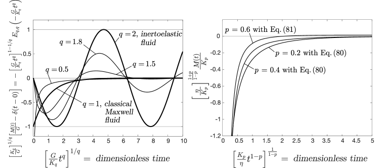
Figure 4: Left: Normalized finite part of the memory function, $\left[\frac{K_{q}}{G}\right]^{\nicefrac{{\text{1}}}{{q}}}\Big{[}\frac{M(t)}{G}$ $-\delta(t-\text{0})$$\Big{]}$ of the spring – Scott-Blair in-series fluid for values $q=$ 0.5, 1, 1.5, 1.8 and 2 as a function of the dimensionless time $\Big{[}\frac{G}{K_{q}}$$t^{q}$$\Big{]}^{\nicefrac{{\text{1}}}{{q}}}$. For $q\leq$ 1 the time-response functions exhibit a monotonically decreasing behavior; whereas for $q>$ 1, they exhibit an oscillatory behavior capable to capture inertia effects. Right: Normalized memory function of the springpot – dashpot in-series fluid. For $p=$ 0.2 and $p=$ 0.4, Eq. (80) was used; whereas for $p=$ 0.6, Eq. (81) was used.

$$E_{\text{2, 2}}\left(-\omega_{R}^{\text{2}}t^{\text{2}}\right)= \frac{\sinh(\operatorname{i}\omega_{R}t)}{\operatorname{i}\omega_{R}t}=$$ (79)

$$\frac{\text{1}}{\omega_{R}t}\frac{e^{\operatorname{i}\omega_{R}t}-e^{-\operatorname{i}\omega_{R}t}}{\text{2}\operatorname{i}}=\frac{\text{1}}{\omega_{R}t}\sin(\omega_{R}t)\text{,}$$

Eq. (78) reduces to $M(t)=G\left[\delta(t-\text{0})-\omega_{R}\sin(\omega_{R}t)\right]$, which is the memory function of a spring – inerter connected in-series (Makris 2017). Figure 4 (left) plots the normalized finite part of Eq. (75), $\frac{M(t)}{G}$ $-\delta(t-\text{0})$, for various values of $q$ as a function of the dimensionless time $\Big{[}\frac{G}{K_{q}}$$t^{q}$$\Big{]}^{\nicefrac{{\text{1}}}{{q}}}$ and shows that when $q>$ 1, the memory function offered by Eq. (75) is capable to capture inertia effects in the rheological network as these manifested in high-frequency microrheology (Domínguez-García et al. 2014; Indei et al. 2012).

2. Springpot – Dashpot in-series $(q=\text{1}$, $r=q-p=\text{1}-p\text{, }K_{q}=\eta)$. For this case where $q=\text{1}$ and $\text{0}\leq p\leq\text{1}$, we first use Eq. (73)

$$M(t)= K_{p}\Bigg{[}\frac{\mathrm{d}^{p}}{\mathrm{d}t^{p}}\delta(t-\text{0})-$$ (80)

$$\frac{K_{p}}{\eta}\frac{\text{1}}{t^{\text{2}p}}E_{\text{1}-p\text{, }\text{1}-\text{2}p}\left(-\frac{K_{p}}{\eta}t^{\text{1}-p}\right)\Bigg{]}\text{,}\enskip\text{0}\leq p\leq\text{1}$$

Eq. (80) is valid for values of $\text{0}\leq p<$ $\nicefrac{{\text{1}}}{{\text{2}}}$. In the event that $p\geq$ $\nicefrac{{\text{1}}}{{\text{2}}}$, the second index of the Mittag-Leffler function remains negative and we need to use the next expression for the memory function given by Eq. (74)

$$M(t)=K_{p}\Bigg{[}\frac{\mathrm{d}^{p}}{\mathrm{d}t^{p}}\delta(t-\text{0})-\frac{K_{p}}{\eta}\frac{\mathrm{d}^{\text{2}p-\text{1}}}{\mathrm{d}t^{\text{2}p-\text{1}}}\delta(t-\text{0})-$$ (81)

$$\left(\frac{K_{p}}{\eta}\right)^{\text{2}}\frac{\text{1}}{t^{\text{3}p-\text{1}}}E_{\text{1}-p\text{, }\text{2}-\text{3}p}\left(-\frac{K_{p}}{\eta}t^{\text{1}-p}\right)\Bigg{]}\text{,}\enskip\text{0}\leq p\leq\text{1}$$

Figure 4 (right) plots the normalized memory function of the springpot – dashpot in-series fluid $\left[\frac{\eta}{K_{p}}\right]^{\frac{\text{1}+p}{\text{1}-p}}\frac{M(t)}{K_{p}}$ for various values of $p$ as a function of the dimensioless time $\Big{[}\frac{K_{p}}{\eta}$$t^{\text{1}-p}$$\Big{]}^{\frac{\text{1}}{\text{1}-p}}$. For $p=$ 0.2 and $p=$ 0.4, Eq. (80) was used; whereas for $p=$ 0.6, Eq. (81) was used.

The complex dynamic compliance $\mathcal{J}(s)=$ $\nicefrac{{\text{1}}}{{\mathcal{G}(s)}}$ derives directly from Eq. (67) in which $r=q-p$ and $\lambda_{r}=$ $\nicefrac{{K_{q}}}{{K_{p}}}$

$$\mathcal{J}(s)=\frac{\text{1}}{K_{q}}\frac{\text{1}+\lambda_{r}s^{q-p}}{s^{q}}=\frac{\text{1}}{K_{p}}\frac{\text{1}}{s^{p}}+\frac{\text{1}}{K_{q}}\frac{\text{1}}{s^{q}}$$ (82)

The impulse fluidity (impulse response function), $\phi(t)$, is the superposition of the impulse fluidities of the two Scott-Blair elements connected in-series

$$\phi(t)= \mathcal{L}^{-\text{1}}\left\{\mathcal{J}(s)\right\}=\Bigg{[}\frac{\text{1}}{K_{p}}\frac{\text{1}}{\Gamma(p)}\frac{\text{1}}{t^{\text{1}-p}}+$$ (83)

$$\frac{\text{1}}{K_{q}}\frac{\text{1}}{\Gamma(q)}\frac{\text{1}}{t^{\text{1}-q}}\Bigg{]}U(t-\text{0})\text{,}\enskip\text{0}<p<q\in\mathbb{R}^{+}$$

Special Cases: 1. Spring – Scott-Blair element in-series $(p=\text{0}$, $r=q-p=q\in\mathbb{R}^{+}\text{, }K_{p}=G)$. In the case where $p=\text{0}$, the first term in the bracket of Eq. (83) becomes the Dirac delta function $\delta(t-\text{0})$ according to Eq. (31) (Gel’fand and Shilov 1964). Consequently, for $p=\text{0}$ and $K_{p}=G$ in association with Eq. (31), Eq. (83) yields

$$\phi(t)=\frac{\text{1}}{G}\delta(t-\text{0})+\frac{\text{1}}{K_{q}}\frac{\text{1}}{\Gamma(q)}\frac{\text{1}}{t^{\text{1}-q}}U(t-\text{0})\text{,}\enskip q\in\mathbb{R}^{+}$$ (84)

which is the superposition of the impulse fluidities of the Hookean spring and that of the Scott-Blair (springpot) element shown in Table 2. When $q=\text{2}$, $K_{q}=K_{\text{2}}=m_{R}$, Eq. (84) gives $\phi(t)=$ $\frac{\text{1}}{G}$$\delta(t-\text{0})+$$\frac{\text{1}}{m_{R}}$$tU(t-\text{0})$, which is the impulse fluidity of a spring – inerter in-series connection (Makris 2017).

2. Springpot – Dashpot in-series $(q=\text{1}$, $r=q-p=\text{1}-p\text{, }K_{q}=\eta)$. In this case where $q=\text{1}$, Eq. (83) yields

$$\phi(t)=\left[\frac{\text{1}}{K_{p}}\frac{\text{1}}{\Gamma(p)}\frac{\text{1}}{t^{\text{1}-p}}+\frac{\text{1}}{\eta}\right]U(t-\text{0})$$ (85)

which is the superposition of the impulse fluidities of the springpot element and that of a dashpot. For the classical limit when $p=\text{0}$, $K_{p}=G$, $q=\text{1}$ and $K_{q}=\eta$, Eq. (84) yields $\phi(t)=$ $\frac{\text{1}}{G}$$\delta(t-\text{0})+$ $\frac{\text{1}}{\eta}$$U(t-\text{0})$ which is the impulse fluidity (impulse response function) of the classical Maxwell model shown in Table 2.

The complex dynamic viscosity (impedance), $\eta(s)$, of the generalized Maxwell fluid derives directly from Eq. (67), since $\eta(s)=$ $\nicefrac{{\mathcal{G}(s)}}{{s}}$

$$\eta(s)=K_{p}\frac{s^{q-\text{1}}}{s^{r}+\nicefrac{{K_{p}}}{{K_{q}}}}=K_{p}\frac{s^{r-(\text{1}-p)}}{s^{r}+\nicefrac{{K_{p}}}{{K_{q}}}}\text{,}\enskip r=q-p>\text{0}$$ (86)

The relaxation modulus, $G(t)$, is the inverse Laplace transform of Eq. (86)

$$G(t)= \mathcal{L}^{-\text{1}}\left\{\mathcal{\eta}(s)\right\}=\mathcal{L}^{-\text{1}}\left\{K_{p}\frac{s^{r-(\text{1}-p)}}{s^{r}+\nicefrac{{K_{p}}}{{K_{q}}}}\right\}=$$ (87)

$$K_{p}\,\frac{\text{1}}{t^{p}}\,E_{r\text{, }\text{1}-p}\left(-\frac{K_{p}}{K_{q}}t^{r}\right)\text{,}\enskip t>\text{0}$$

and by replacing $r=q-p$,

$$G(t)=K_{p}\,\frac{\text{1}}{t^{p}}\,E_{q-p\text{, }\text{1}-p}\left(-\frac{K_{p}}{K_{q}}t^{q-p}\right)\text{,}\enskip\text{0}<p<q\in\mathbb{R}^{+}$$ (88)

The expression given by Eq. (88) has been presented by Friedrich (1991); Schiessel et al. (1995); Palade et al. (1996) and was employed by Jaishankar and McKinley (2013)

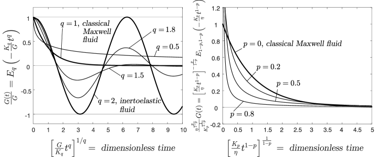
Figure 5: Left: Normalized relaxation modulus $\frac{G(t)}{G}$ of the spring – Scott-Blair in-series fluid for values $q=$ 0.5, 1, 1.5, 1.8 and 2 as a function of the dimensionless time $\Big{[}\frac{G}{K_{q}}$$t^{q}$$\Big{]}^{\nicefrac{{\text{1}}}{{q}}}$. For $q\leq$ 1, the time-response functions exhibit a monotonically decreasing behavior; whereas for $q>$ 1, they exhibit an oscillatory behavior capable to capture inertia effects. Figure 4 (left) has been presented by Glöckle and Nonnenmacher (1994) by merely allowing $q$ to assume values larger than 1, about a decade before the concept of the inerter and its equivalence to the electric capacitor was established by Smith (2002). Right: Normalized relaxation modulus of the springpot – dashpot in-series fluid for values of $p=$ 0, 0.2, 0.5 and 0.8 as a function of the dimensionless time $\Big{[}\frac{K_{p}}{\eta}$$t^{\text{1}-p}$$\Big{]}^{\frac{\text{1}}{\text{1}-p}}$ with 0 $\leq p\leq$ 1.

Special Cases: 1. Spring – Scott-Blair element in-series $(p=\text{0}$, $r=q-p=q\in\mathbb{R}^{+}\text{, }K_{p}=G)$. In this case where $p=\text{0}$, Eq. (88) reduces to

$$G(t)= G\,E_{q\text{, 1}}\left(-\frac{G}{K_{q}}t^{q}\right)=$$ (89)

$$G\,E_{q}\left(-\frac{G}{K_{q}}t^{q}\right)\text{,}\enskip q\in\mathbb{R}^{+}$$

The result of Eq. (89) has been presented by Koeller (1984); Schiessel et al. (1995); Mainardi and Spada (2011). When $q=\text{1}$, the Mittag-Leffler function $E_{\text{1}}\Big{(}-$ $\frac{G}{\eta}$$t\Big{)}$ reduces to the exponential function $e^{-}$${}^{\nicefrac{{t}}{{\lambda}}}$ where $\lambda=$ $\nicefrac{{\eta}}{{G}}$ $=$ relaxation time; and Eq. (89) gives the relaxation modulus of the classical Maxwell model $G(t)=Ge^{-}$${}^{\nicefrac{{t}}{{\lambda}}}$. When $q=\text{2}$, $K_{q}=K_{\text{2}}=m_{R}$ and $\frac{G}{K_{\text{2}}}$ $=$ $\frac{G}{m_{R}}$ $=\omega_{R}^{\text{2}}$. By virtue of the identity $E_{\text{2, 1}}\left(-\omega_{R}^{\text{2}}t^{\text{2}}\right)=E_{\text{2}}\left(-\omega_{R}^{\text{2}}t^{\text{2}}\right)=\cos(\omega_{R}^{\text{2}}t)$, Eq. (89) reduces to $G(t)=G\cos(\omega_{R}t)$ which is the relaxation modulus of a spring – inerter connected in-series (Makris 2017). The emerging of the $\cos$ine function (oscillatory behavior) when $q=$ 2 has been reported by Glöckle and Nonnenmacher (1994) after examining the solutions of the Fox H-function that is related to the Mittag-Leffler function. The oscillatory behavior of the relaxation modulus, $G(t)$, when $q=$ 2 is the result of the continuous exchange of potential and kinetic energies between the spring $(p=\text{0})$ and the inerter $(q=\text{2})$. Figure 5 (left) plots the relaxation modulus given by Eq. (89) for various values of $q$ as a function of the dimensionless time $\Big{[}\frac{G}{K_{q}}$$t^{q}$$\Big{]}^{\nicefrac{{\text{1}}}{{q}}}$.

2. Springpot – Dashpot in-series $(q=\text{1}$, $r=q-p=\text{1}-p\text{, }K_{q}=\eta)$. In this case where $q=\text{1}$, Eq. (88) reduces to

$$G(t)=K_{p}\,\frac{\text{1}}{t^{p}}\,E_{\text{1}-p\text{, }\text{1}-p}\left(-\frac{K_{p}}{\eta}t^{\text{1}-p}\right)\text{,}\enskip\text{0}\leq p\leq\text{1}$$ (90)

Figure 5 (right) plots the normalized relaxation modulus, $G(t)$, of the springpot – dashpot in-series element for various values of $p$ $(\text{0}\leq p\leq\text{1})$.

The complex dynamic fluidity (admittance), $\phi(s)$, of the generalized fractional Maxwell fluid is the inverse of the complex dynamic viscosity given by Eq. (86)

$$\phi(s)= \frac{\text{1}}{K_{p}}\frac{s^{r}+\nicefrac{{K_{p}}}{{K_{q}}}}{s^{q-\text{1}}}=$$ (91)

$$\frac{\text{1}}{K_{p}}s^{\text{1}-p}+\frac{\text{1}}{K_{q}}s^{\text{1}-q}\text{,}\enskip r=q-p>\text{0}$$

The impulse strain-rate response function of the generalized fractional Maxwell fluid, $\psi(t)$, is the superposition of the impulse strain-rate response functions of the two Scott-Blair elements connected in-series

$$\psi(t)= \mathcal{L}^{-\text{1}}\left\{\phi(s)\right\}=\Bigg{[}\frac{\text{1}}{K_{p}}\frac{\text{1}}{\Gamma(-\text{1}+p)}\frac{\text{1}}{t^{\text{2}-p}}+$$ (92)

$$\frac{\text{1}}{K_{q}}\frac{\text{1}}{\Gamma(-\text{1}+q)}\frac{\text{1}}{t^{\text{2}-q}}\Bigg{]}U(t-\text{0})\text{,}\enskip\text{0}<p<q\in\mathbb{R}^{+}$$

Special Cases: 1. Spring – Scott-Blair element in-series $(p=\text{0}$, $r=q-p=q\in\mathbb{R}^{+}\text{, }K_{p}=G)$. In this case where $p=\text{0}$, the first term in the bracket of Eq. (92) becomes equal to the first derivative of the Dirac delta function, $\frac{\mathrm{d}\delta(t-\text{0})}{\mathrm{d}t}$, according to Eq. (31). Consequently for $p=\text{0}$ and $K_{p}=G$, in association with Eq. (31), Eq. (92) yields

$$\psi(t)=\frac{\text{1}}{G}\frac{\mathrm{d}\delta(t-\text{0})}{\mathrm{d}t}+\frac{\text{1}}{K_{q}}\frac{\text{1}}{\Gamma(-\text{1}+q)}\frac{\text{1}}{t^{\text{2}-q}}U(t-\text{0})$$ (93)

2. Springpot – Dashpot in-series: $(q=\text{1}$, $r=q-p=\text{1}-p\text{, }K_{q}=\eta)$. In this case where $q=\text{1}$, the second term in the bracket of Eq. (92) becomes equal to the Dirac delta function, $\delta(t-\text{0})$, according to Eq. (31). Consequently for $q=\text{1}$ and $K_{q}=\eta$, in association with Eq. (31), Eq. (92) yields

$$\psi(t)=\frac{\text{1}}{K_{p}}\frac{\text{1}}{\Gamma(-\text{1}+p)}\frac{\text{1}}{t^{\text{2}-p}}U(t-\text{0})+\frac{\text{1}}{\eta}\delta(t-\text{0})$$ (94)

The complex creep function, $\mathcal{C}(\omega)$, of the generalized fractional Maxwell fluid derives directly from Eq. (82) given that $\mathcal{C}(s)=$ $\nicefrac{{\mathcal{J}(s)}}{{s}}$

$$\mathcal{C}(s)=\frac{\text{1}}{K_{q}}\frac{\text{1}+\lambda_{r}s^{q-p}}{s^{\text{1}+q}}=\frac{\text{1}}{K_{p}}\frac{\text{1}}{s^{\text{1}+p}}+\frac{\text{1}}{K_{q}}\frac{\text{1}}{s^{\text{1}+q}}$$ (95)

Table 3: Frequency-response functions and the corresponding causal time-response functions of the generalized fractional derivative Maxwell fluid and of its special cases.

	Generalized Fractional Derivative Maxwell Fluid	Spring – Scott-Blair In-Series Connection	Springpot – Dashpot In-Series Connection
Constitutive Equation	$\tau(t)+\cfrac{K_{q}}{K_{p}}\cfrac{\mathrm{d}^{q-p}}{\mathrm{d}t^{q-p}}\tau(t)=K_{q}\cfrac{\mathrm{d}^{q}\gamma(t)}{\mathrm{d}t^{q}}$	$\tau(t)+\cfrac{K_{q}}{G}\cfrac{\mathrm{d}^{q}\tau(t)}{\mathrm{d}t^{q}}=K_{q}\cfrac{\mathrm{d}^{q}\gamma(t)}{\mathrm{d}t^{q}}$	$\tau(t)+\cfrac{\eta}{K_{q}}\cfrac{\mathrm{d}^{\text{1}-q}}{\mathrm{d}t^{\text{1}-q}}\tau(t)=\eta\cfrac{\mathrm{d}\gamma(t)}{\mathrm{d}t}$
Complex Dynamic Modulus $\mathcal{G}(\omega)=\frac{\tau(\omega)}{\gamma(\omega)}$	$K_{q}\cfrac{(\operatorname{i}\omega)^{q}}{\text{1}+\frac{K_{q}}{K_{p}}(\operatorname{i}\omega)^{q-p}}$	$K_{q}\cfrac{(\operatorname{i}\omega)^{q}}{\text{1}+\frac{K_{q}}{G}(\operatorname{i}\omega)^{q}}$	$\eta\cfrac{\operatorname{i}\omega}{\text{1}+\frac{\eta}{K_{q}}(\operatorname{i}\omega)^{\text{1}-q}}$
Complex Dynamic Viscosity $\mathcal{\eta}(\omega)=\frac{\tau(\omega)}{\accentset{\mbox{\large.}}{\gamma}(\omega)}$	$K_{p}\cfrac{(\operatorname{i}\omega)^{q-\text{1}}}{(\operatorname{i}\omega)^{q-p}+\frac{K_{p}}{K_{q}}}$	$G\cfrac{(\operatorname{i}\omega)^{q}}{\operatorname{i}\omega\left[(\operatorname{i}\omega)^{q}+\frac{G}{K_{q}}\right]}$	$\cfrac{\eta}{\text{1}+\frac{\eta}{K_{q}}(\operatorname{i}\omega)^{\text{1}-q}}$
Complex Dynamic Compliance $\mathcal{J}(\omega)=\frac{\text{1}}{\mathcal{G}(\omega)}=\frac{\gamma(\omega)}{\tau(\omega)}$	$\cfrac{\text{1}}{K_{p}}\cfrac{\text{1}}{(\operatorname{i}\omega)^{p}}+\cfrac{\text{1}}{K_{q}}\cfrac{\text{1}}{(\operatorname{i}\omega)^{q}}$	$\cfrac{\text{1}}{G}+\cfrac{\text{1}}{K_{q}}\cfrac{\text{1}}{(\operatorname{i}\omega)^{q}}$	$\cfrac{\text{1}}{\eta}\left[\pi\delta(\omega-\text{0})-\operatorname{i}\cfrac{\text{1}}{\omega}\right]+\cfrac{\text{1}}{K_{q}}\cfrac{\text{1}}{(\operatorname{i}\omega)^{q}}$
Complex Creep Function $\mathcal{C}(\omega)=\frac{\gamma(\omega)}{\accentset{\mbox{\large.}}{\tau}(\omega)}$	$\cfrac{\text{1}}{K_{p}}\cfrac{\text{1}}{(\operatorname{i}\omega)^{\text{1}+p}}+\cfrac{\text{1}}{K_{q}}\cfrac{\text{1}}{(\operatorname{i}\omega)^{\text{1}+q}}$	$\cfrac{\text{1}}{G}\left[\pi\delta(\omega-\text{0})-\operatorname{i}\cfrac{\text{1}}{\omega}\right]+\cfrac{\text{1}}{K_{q}}\cfrac{\text{1}}{(\operatorname{i}\omega)^{q+\text{1}}}$	$\cfrac{\text{1}}{\eta}\left[-\cfrac{\text{1}}{\omega^{\text{2}}}+\operatorname{i}\pi\cfrac{\mathrm{d}\delta(\omega-\text{0})}{\mathrm{d}\omega}\right]+\cfrac{\text{1}}{K_{q}}\cfrac{\text{1}}{(\operatorname{i}\omega)^{q+\text{1}}}$
Complex Dynamic Fluidity $\mathcal{\phi}(\omega)=\frac{\text{1}}{\eta(\omega)}=\frac{\accentset{\mbox{\large.}}{\gamma}(\omega)}{\tau(\omega)}$	$\cfrac{\text{1}}{K_{p}}(\operatorname{i}\omega)^{\text{1}-p}+\cfrac{\text{1}}{K_{q}}(\operatorname{i}\omega)^{\text{1}-q}$	$\cfrac{\text{1}}{G}\operatorname{i}\omega+\cfrac{\text{1}}{K_{q}}(\operatorname{i}\omega)^{\text{1}-q}$	$\cfrac{\text{1}}{K_{q}}(\operatorname{i}\omega)^{\text{1}-q}+\cfrac{\text{1}}{\eta}$
Memory Function $M(t)$	$\cfrac{K_{p}}{t^{p+\text{1}}}\Bigg{[}\cfrac{\text{1}}{\Gamma(-p)}U(t-\text{0})-\quad\quad\quad\quad\quad\quad$ $\quad\quad\quad\quad\cfrac{K_{p}}{K_{q}}\cfrac{\text{1}}{t^{p-q}}E_{q-p\text{, }q-\text{2}p}\left(-\cfrac{K_{p}}{K_{q}}t^{q-p}\right)\Bigg{]}$	$G\left[\delta(t-\text{0})-\cfrac{G}{K_{q}}\cfrac{\text{1}}{t^{\text{1}-q}}E_{q\text{, }q}\left(-\cfrac{G}{K_{q}}t^{q}\right)\right]$	$\cfrac{K_{q}}{t^{q+\text{1}}}\Bigg{[}\cfrac{\text{1}}{\Gamma(-q)}U(t-\text{0})-\quad\quad\quad\quad\quad\quad\quad\quad\quad$ $\quad\quad\cfrac{K_{q}}{\eta}\cfrac{\text{1}}{t^{q-\text{1}}}E_{\text{1}-q\text{, }\text{1}-\text{2}q}\left(-\cfrac{K_{q}}{\eta}t^{\text{1}-q}\right)\Bigg{]}$
Relaxation Modulus $G(t)$	$K_{p}\,\cfrac{\text{1}}{t^{p}}\,E_{q-p\text{, }\text{1}-p}\left(-\cfrac{K_{p}}{K_{q}}t^{q-p}\right)$	$G\,E_{q}\left(-\cfrac{G}{K_{q}}t^{q}\right)$	$K_{q}\,\cfrac{\text{1}}{t^{q}}\,E_{\text{1}-q\text{, }\text{1}-q}\left(-\cfrac{K_{q}}{\eta}t^{\text{1}-q}\right)$
Impulse Fluidity $\phi(t)$	$\left[\cfrac{\text{1}}{K_{p}}\cfrac{\text{1}}{\Gamma(p)}\cfrac{\text{1}}{t^{\text{1}-p}}+\cfrac{\text{1}}{K_{q}}\cfrac{\text{1}}{\Gamma(q)}\cfrac{\text{1}}{t^{\text{1}-q}}\right]U(t-\text{0})$	$\cfrac{\text{1}}{G}\,\delta(t-\text{0})+\cfrac{\text{1}}{K_{q}}\cfrac{\text{1}}{\Gamma(q)}\cfrac{\text{1}}{t^{\text{1}-q}}U(t-\text{0})$	$\left[\cfrac{\text{1}}{K_{q}}\cfrac{\text{1}}{\Gamma(q)}\cfrac{\text{1}}{t^{\text{1}-q}}+\cfrac{\text{1}}{\eta}\right]U(t-\text{0})$
Creep Compliance $J(t)$	$\left[\cfrac{\text{1}}{K_{p}}\cfrac{t^{p}}{\Gamma(p+\text{1})}+\cfrac{\text{1}}{K_{q}}\cfrac{t^{q}}{\Gamma(q+\text{1})}\right]U(t-\text{0})$	$\left[\cfrac{\text{1}}{G}+\cfrac{\text{1}}{K_{q}}\cfrac{t^{q}}{\Gamma(q+\text{1})}\right]U(t-\text{0})$	$\left[\cfrac{\text{1}}{K_{q}}\cfrac{\text{1}}{\Gamma(q+\text{1})}t^{q}+\cfrac{\text{1}}{\eta}t\right]U(t-\text{0})$
Impulse Strain-rate Response Function $\psi(t)$	$\left[\cfrac{\text{1}}{K_{p}}\cfrac{\text{1}}{\Gamma(-\text{1}+p)}\cfrac{\text{1}}{t^{\text{2}-p}}+\cfrac{\text{1}}{K_{q}}\cfrac{\text{1}}{\Gamma(-\text{1}+q)}\cfrac{\text{1}}{t^{\text{2}-q}}\right]U(t-\text{0})$	$\cfrac{\text{1}}{G}\cfrac{\mathrm{d}\delta(t-\text{0})}{\mathrm{d}t}+\cfrac{\text{1}}{K_{q}}\cfrac{\text{1}}{\Gamma(-\text{1}+q)}\cfrac{\text{1}}{t^{\text{2}-q}}U(t-\text{0})$	$\cfrac{\text{1}}{K_{q}}\cfrac{\text{1}}{\Gamma(-\text{1}+q)}\cfrac{\text{1}}{t^{\text{2}-q}}U(t-\text{0})+\cfrac{\text{1}}{\eta}\delta(t-\text{0})$

The creep compliance (retardation function), $J(t)$, is the superposition of the creep compliances of the two Scott-Blair elements connected in-series.

$$J(t)= \mathcal{L}^{-\text{1}}\left\{\mathcal{C}(s)\right\}=$$ (96)

$$\left[\frac{\text{1}}{K_{p}}\frac{t^{p}}{\Gamma(p+\text{1})}+\frac{\text{1}}{K_{q}}\frac{t^{q}}{\Gamma(q+\text{1})}\right]U(t-\text{0})$$

The expression given by Eq. (96) has been presented by Friedrich (1991); Schiessel et al. (1995); Jaishankar and McKinley (2013); Hristov (2019).

Special Cases: 1. Spring – Scott-Blair element in-series $(p=\text{0}$, $r=q-p=q\in\mathbb{R}^{+}\text{, }K_{p}=G)$. In this case where $p=\text{0}$, Eq. (96) reduces to

$$J(t)=\left[\frac{\text{1}}{G}+\frac{\text{1}}{K_{q}}\frac{t^{q}}{\Gamma(q+\text{1})}\right]U(t-\text{0})$$ (97)

The result of Eq. (97) has been presented by Koeller (1984); Schiessel et al. (1995); Mainardi and Spada (2011).

2. Springpot – Dashpot in-series $(q=\text{1}$, $r=q-p=\text{1}-p\text{, }K_{q}=\eta)$. In this case where $p=\text{1}$, Eq. (96) reduces to

$$J(t)=\left[\frac{\text{1}}{K_{p}}\frac{t^{p}}{\Gamma(p+\text{1})}+\frac{\text{1}}{\eta}t\right]U(t-\text{0})$$ (98)

For the classical limit when $p=\text{0}$, $K_{p}=G$, $q=\text{1}$ and $K_{q}=\eta$, Eq. (96) yields $J(t)=$ $\Big{[}\frac{\text{1}}{G}+\frac{\text{1}}{\eta}$$t$$\Big{]}$$U(t-\text{0})$ which is the creep compliance of the classical Maxwell fluid shown in Table 2.

The five causal time-response functions of the generalized fractional Maxwell fluid together with the time-response functions for the special cases of the spring – Scott-Blair element in-series connection $(p=\text{0})$ and the springpot – dashpot in-series connection $(q=\text{1})$ are summarized in Table 3.

7 Time-response function of the generalized fractional Kelvin-Voigt element

The parallel connection of the two Scott-Blair elements shown in Figure 3 (right) exhibits a solid-like behavior only when $p=\text{0}$ or $q=\text{0}$. In any other situation where $p>\text{0}$ and $q>\text{0}$, the generalized fractional Kelvin-Voigt element shown in Figure 3 (right) exhibits a fluid-like behavior since it results in infinite deformation under a static load. In view of this behavior the term “generalized” fractional Kelvin-Voigt element is used for the viscoelastic model shown in Figure 3 (right) with constitutive law

$$\tau(t)=K_{p}\frac{\mathrm{d}^{p}\gamma(t)}{\mathrm{d}t^{p}}+K_{q}\frac{\mathrm{d}^{q}\gamma(t)}{\mathrm{d}t^{q}}\text{,}\enskip p\text{, }q\in\mathbb{R}^{+}$$ (99)

When $p=$ 0, the generalized fractional Kelvin-Voigt element given by Eq. (99) reduces to a spring – Scott-Blair element parallel connection — a model that was proposed by Suki et al. (1994) to express the pressure–volume relation of the lung tissue viscoelastic behavior of human and selective animal lungs. The same spring – Scott-Blair element was subsequently used by Puig-de-Morales-Marinkovic et al. (2007) to model the viscoelastic behavior of the human red blood cells. When $(\text{0}\leq p\leq\text{1 and }q=\text{1})$ the generalized fractional Kelvin-Voigt element given by Eq. (99) reduces to a springpot – dashpot parallel connection — a model that has been used to capture the high-frequency behavior of semiflexible polymer networks (Gittes and MacKintosh 1998; Atakhorrami et al. 2008; Domínguez-García et al. 2014).

Because of the parallel arrangement of the two Scott-Blair elements, the memory function, $M(t)$, of the generalized fractional Kelvin-Voigt element is the summation of the memory functions of the two individual Scott-Blair elements given by Eq. (36)

$$M(t)= \left[\frac{K_{p}}{\Gamma(-p)}\frac{\text{1}}{t^{p+1}}+\frac{K_{q}}{\Gamma(-q)}\frac{\text{1}}{t^{q+1}}\right]U(t-\text{0})=$$ (100)

$$K_{p}\frac{\mathrm{d}^{p}\delta(t-\text{0})}{\mathrm{d}t^{p}}+K_{q}\frac{\mathrm{d}^{q}\delta(t-\text{0})}{\mathrm{d}t^{q}}$$

Special Cases: 1. Spring – Scott-Blair element in parallel $(p=\text{0}$, $q\in\mathbb{R}^{+}\text{, }K_{p}=G)$.

$$M(t)=G\delta(t-\text{0})+\frac{K_{q}}{\Gamma(-q)}\frac{\text{1}}{t^{q+\text{1}}}U(t-\text{0})$$ (101)

2. Springpot – Dashpot in parallel $(p\in\mathbb{R}^{+}$, $q=\text{1}$, $K_{q}=\eta)$.

$$M(t)=\frac{K_{p}}{\Gamma(-p)}\frac{\text{1}}{t^{p+\text{1}}}U(t-\text{0})+\eta\frac{\mathrm{d}\delta(t-\text{0})}{\mathrm{d}t}$$ (102)

For the classical limit when $p=\text{0}$, $K_{p}=G$, $q=\text{1}$ and $K_{q}=\eta$, Eq. (100) yields $M(t)=G\delta(t-\text{0})+\eta$$\frac{\mathrm{d}\delta(t-\text{0})}{\mathrm{d}t}$ which is the memory function of the classical Kelvin-Voigt solid shown in Table 2. When $q=$ 2 and $K_{q}=K_{\text{2}}=m_{R}$, Eq. (101) yields $M(t)=G\delta(t-\text{0})+m_{R}$$\frac{\mathrm{d}^{\text{2}}\delta(t-\text{0})}{\mathrm{d}t^{\text{2}}}$, which is the memory function of the inerto-elastic solid (Makris 2017).

The complex dynamic compliance, $\mathcal{J}(\omega)=$ $\nicefrac{{\gamma(\omega)}}{{\tau(\omega)}}$, derives directly from the Fourier transform of Eq. (99), $\tau(\omega)=\left[K_{p}(\operatorname{i}\omega)^{p}+K_{q}(\operatorname{i}\omega)^{q}\right]\gamma(\omega)$ and by using the Laplace variable $s=\operatorname{i}\omega$

$$\mathcal{J}(s)= \frac{\gamma(s)}{\tau(s)}=\frac{\text{1}}{K_{p}s^{p}+K_{q}s^{q}}=$$ (103)

$$\frac{\text{1}}{K_{p}}\frac{\text{1}}{s^{p}\left(\text{1}+\frac{K_{q}}{K_{p}}s^{q-p}\right)}=\frac{\text{1}}{K_{q}}\frac{\text{1}}{s^{p}\left(s^{r}+\frac{K_{p}}{K_{q}}\right)}\text{,}$$

$$\quad\quad\quad\quad\quad\quad\quad\quad\quad\quad\quad\quad\text{with}\enskip p\text{, }r\in\mathbb{R}^{+}$$

where without loss of generality we set $r=q-p>\text{0}$. The inverse Laplace transform of Eq. (103) is evaluated with the convolution integral given by Eq. (68), where

$$f(t)= \mathcal{L}^{-\text{1}}\left\{\mathcal{F}(s)\right\}=\mathcal{L}^{-\text{1}}\left\{\frac{\text{1}}{K_{q}}\frac{\text{1}}{s^{p}}\right\}=$$ (104)

$$\frac{\text{1}}{K_{q}}\frac{\text{1}}{\Gamma(p)}t^{p-\text{1}}\text{,}\enskip p\in\mathbb{R}^{+}$$

and $h(t)=\mathcal{L}^{-\text{1}}\left\{\mathcal{H}(s)\right\}$ is given by Eq. (70). Substitution of the results of Eqs. (104) and (70) into the convolution integral given by Eq. (68), the impulse fluidity (impulse response function) of the generalized fractional Kelvin-Voigt element is

$$\phi(t)= \mathcal{L}^{-\text{1}}\left\{\mathcal{J}(s)\right\}=$$ (105)

$$\frac{\text{1}}{K_{q}}\frac{\text{1}}{\Gamma(p)}\int_{\text{0}}^{t}(t-\xi)^{p-\text{1}}\xi^{r-\text{1}}E_{r\text{, }r}\left(-\frac{K_{p}}{K_{q}}\xi^{r}\right)\mathrm{d}\xi$$

Eq. (105) shows that the impulse fluidity, $\phi(t)$, of the generalized Kelvin-Voigt model is merely the fractional integral of order $p$ (see Eq. (3)) of the function given by Eq. (70) $(r=q-p)$

$$\phi(t)= \frac{\text{1}}{K_{q}}I^{p}\left[\frac{\text{1}}{t^{\text{1}-p+q}}E_{q-p\text{, }q-p}\left(-\frac{K_{p}}{K_{q}}t^{q-p}\right)\right]=$$ (106)

$$\frac{\text{1}}{K_{q}}\frac{\text{1}}{t^{\text{1}-q}}E_{q-p\text{, }q}\left(-\frac{K_{p}}{K_{q}}t^{q-p}\right)$$

where the right-hand side of Eq. (106) was evaluated by using the general result offered by Eq. (58) with $\alpha=\beta=q-p$.

Special Cases: 1. Spring – Scott-Blair element in parallel $(p=\text{0}$, $q\in\mathbb{R}^{+}\text{, }K_{p}=G)$. In this case, Eq. (106) for $p=$ 0 gives

$$\phi(t)=\frac{\text{1}}{K_{q}}\frac{\text{1}}{t^{\text{1}-q}}E_{q\text{, }q}\left(-\frac{G}{K_{q}}t^{q}\right)\text{,}\enskip q\in\mathbb{R}^{+}$$ (107)

At the same time, the reader recognizes that for $p=\text{0}$, the coefficient of the fractional integral given by Eq. (105) vanishes since $\frac{\text{1}}{\Gamma(\text{0})}$ $=\text{0}$. Nevertheless, the first term under the integral $\left[\Gamma(p)(t-\xi)\right]^{-\text{1}}$ is the definition of the Dirac delta function given by Eq. (31) (Gel’fand and Shilov 1964). Accordingly, Eq. (105) reduces to

$$\phi(t)= \frac{\text{1}}{K_{q}}\int_{\text{0}}^{t}\delta(\xi-t)\frac{\text{1}}{\xi^{\text{1}-q}}E_{q\text{, }q}\left(-\frac{G}{K_{q}}\xi^{q}\right)\mathrm{d}\xi=$$ (108)

$$\frac{\text{1}}{K_{q}}\frac{\text{1}}{t^{\text{1}-q}}E_{q\text{, }q}\left(-\frac{G}{K_{q}}t^{q}\right)\text{,}\enskip q\in\mathbb{R}^{+}$$

which is the same result offered by Eq. (107). When $q=$ 1, $K_{q}=K_{\text{1}}=\eta$, the impulse fluidity given by Eq. (108) gives $\phi(t)=$ $\frac{\text{1}}{\eta}$$E_{\text{1, 1}}\Big{(}-$$\frac{G}{\eta}$$t\Big{)}$. Using the identity of the Mittag-Leffler function that $E_{\text{1, 1}}(z)=E_{\text{1}}(z)=e^{z}$, together with $\nicefrac{{\eta}}{{G}}$ $=\lambda=$ relaxation time, $\phi(t)=$ $\frac{\text{1}}{\eta}$$e$${}^{-\nicefrac{{t}}{{\lambda}}}$ which is the impulse fluidity of the classical Kelvin-Voigt solid shown in Table 2. When $q=$ 2, $K_{q}=K_{\text{2}}=m_{R}$ is the distributed inertance of an inerter connected in parallel with a spring with elastic constant $G$. In this case Eq. (108) gives $\phi(t)=$ $\frac{\text{1}}{m_{R}}$$tE_{\text{2, 2}}\Big{(}-$$\frac{G}{m_{R}}$$t^{\text{2}}\Big{)}$. By using that $\frac{G}{m_{R}}$ $=\omega_{R}^{\text{2}}$, where $\omega_{R}$ is the rotational frequency of a spring – inerter parellel connection together with the identity given by Eq. (79), $\phi(t)=$ $\frac{\text{1}}{m_{R}\omega_{R}}$$\sin(\omega_{R}t)$, which is the impulse fluidity of a spring – inerter parallel connection (Makris 2017). Eq. (108) is re-written in its dimensionless form

$$\left[\frac{K_{q}}{G}\right]^{\nicefrac{{\text{1}}}{{q}}}G\phi(t)=\left[\frac{G}{K_{q}}t^{q}\right]^{\text{1}-\nicefrac{{\text{1}}}{{q}}}E_{q\text{, }q}\left(-\frac{G}{K_{q}}t^{q}\right)\text{,}\enskip q\in\mathbb{R}^{+}$$ (109)

The plots of the right-hand side of Eq. (109) with a negative sign are depicted in Figure 4 (left) for values of $q=$ 0.5, 1, 1.5, 1.8 and 2 as a function of the dimensionless time $\Big{[}\frac{G}{K_{q}}$$t^{q}$$\Big{]}^{\nicefrac{{\text{1}}}{{q}}}$.

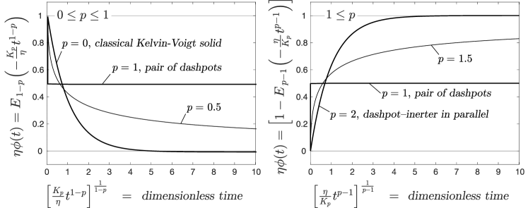
Figure 6: Normalized impulse fluidity (impulse response function) of the Scott-Blair – dashpot parallel connection. The left plots are for $\text{0}\leq p\leq\text{1}$ (springpot – dashpot in parallel), whereas the right plots are for the Scott-Blair – dashpot fluid with $p>$ 1.

2. Scott-Blair – Dashpot in parallel $(p\in\mathbb{R}^{+}$, $q=\text{1}$, $K_{q}=\eta)$. In this case where $q=\text{1}$, the fractional integral of Eq. (106) gives

$$\phi(t)= \frac{\text{1}}{\eta}I^{p}\left[\frac{\text{1}}{t^{p}}E_{\text{1}-p\text{, }\text{1}-p}\left(-\frac{K_{p}}{\eta}t^{\text{1}-p}\right)\right]=$$ (110)

$$\frac{\text{1}}{\eta}E_{\text{1}-p}\left(-\frac{K_{p}}{\eta}t^{\text{1}-p}\right)$$

The result of Eq. (110) is valid only for 0 $\leq p\leq$ 1 (springpot – dashpot connection in parallel). When $p=$ 1, $K_{p}=K_{\text{1}}=\eta_{\text{1}}$ and according to Eq. (110), $\phi(t)=$ $\frac{\text{1}}{\eta}$$E_{\text{0}}$ $\left(-\frac{\eta_{\text{1}}}{\eta}\right)$, which in association with the identity $E_{\text{0}}(-z)=$ $\frac{\text{1}}{\text{1}+z}$, Eq. (110) yields $\phi(t)=$ $\frac{\text{1}}{\eta+\eta_{\text{1}}}$$U(t-\text{0})$, which is the impulse fluidity of two dashpots connected in parallel. When $p>$ 1 the impulse fluidity of the Scott-Blair element – dashpot parallel connection can be obtained by returning to Eq. (103) and setting $q=$ 1 and $K_{q}=\eta$

$$\mathcal{J}(s)=\frac{\text{1}}{K_{p}}\frac{\text{1}}{s\left(s^{p-\text{1}}+\nicefrac{{\eta}}{{K_{p}}}\right)}=\frac{\text{1}}{\eta}\frac{\nicefrac{{\eta}}{{K_{p}}}}{s\left(s^{p-\text{1}}+\nicefrac{{\eta}}{{K_{p}}}\right)}$$ (111)

For $p-\text{1}\geq$ 0, the inverse Laplace transform of Eq. (111) is known

$$\phi(t)= \mathcal{L}^{-\text{1}}\left\{\mathcal{J}(s)\right\}=\mathcal{L}^{-\text{1}}\left\{\frac{\text{1}}{\eta}\frac{\nicefrac{{\eta}}{{K_{p}}}}{s\left(s^{p-\text{1}}+\nicefrac{{\eta}}{{K_{p}}}\right)}\right\}=$$ (112)

$$\frac{\text{1}}{\eta}\left[\text{1}-E_{p-\text{1}}\left(-\frac{\eta}{K_{p}}t^{p-\text{1}}\right)\right]\text{,}\enskip\text{1}\leq p\in\mathbb{R}$$

Eq. (112) offers the impulse fluidity of the Scott-Blair element – dashpot parallel connection when $p\geq$ 1. When $p=$ 1, $K_{p}=K_{\text{1}}=\eta_{\text{1}}$ and according to Eq. (112), $\phi(t)=$ $\frac{\text{1}}{\eta}$$\Big{[}\text{1}-E_{\text{0}}\Big{(}-$$\frac{\eta}{\eta_{\text{1}}}$$\Big{)}\Big{]}$ which in association with the identity $E_{\text{0}}(-z)=$ $\frac{\text{1}}{\text{1}+z}$, Eq. (112) yields $\phi(t)=$ $\frac{\text{1}}{\eta+\eta_{\text{1}}}$$U(t-\text{0})$, which is the result of Eq. (110) for $p=$ 1 and the continuity of the two solutions is established. When $p=$ 2, $K_{p}=K_{\text{2}}=m_{R}$, $\phi(t)=$ $\frac{\text{1}}{\eta}$$\Big{[}\text{1}-E_{\text{1}}\Big{(}-$$\frac{\eta}{m_{R}}$$t\Big{)}\Big{]}$ $=$ $\frac{\text{1}}{\eta}\Big{[}$$U(t-\text{0})-e$${}^{-\frac{\eta}{m_{R}}t}\Big{]}$, which is the impulse fluidity of a dashpot – inerter parallel connection (Makris 2017).

Figure 6 plots the dimensionless impulse fluidity, $\eta\phi(t)$, of the Scott-Blair – dashpot parallel connection for values of $p=$ 0, 0.5, 1, 1.5 and 2 by employing Eq. (110) when $\text{0}\leq p\leq\text{1}$ and Eq. (112) for $\text{1}\leq p$.

Given the parallel connection of the two Scott-Blair elements, the relaxation modulus, $G(t)$, of the generalized fractional Kelvin-Voigt element is the summation of the relaxation moduli of the two individual Scott-Blair elements given by Eq. (49)

$$G(t)=\left[\frac{K_{p}}{\Gamma(\text{1}-p)}\frac{\text{1}}{t^{p}}+\frac{K_{q}}{\Gamma(\text{1}-q)}\frac{\text{1}}{t^{q}}\right]U(t-\text{0})$$ (113)

Special Cases: 1. Spring – Scott-Blair element in parallel $(p=\text{0}$, $q\in\mathbb{R}^{+}\text{, }K_{p}=G)$

$$G(t)=\left[G+K_{q}\frac{\text{1}}{\Gamma(\text{1}-q)}\frac{\text{1}}{t^{q}}\right]U(t-\text{0})$$ (114)

The result of Eq. (114) has been first presented by Koeller (1984).

2. Springpot – Dashpot in parallel $(q=\text{1}$, $K_{q}=\eta)$

$$G(t)=K_{p}\frac{\text{1}}{\Gamma(\text{1}-p)}\frac{\text{1}}{t^{p}}U(t-\text{0})+\eta\delta(t-\text{0})$$ (115)

The Dirac delta function in the right-hand side of Eq. (115) emerges by virtue of Eq. (31) for $n=\text{0}$.

The complex dynamic fluidity (admittance), $\phi(s)$, of the generalized fractional Kelvin-Voigt element derives directly from Eq. (103) by using that $\accentset{\mbox{\large.}}{\gamma}(s)=s\gamma(s)$

$$\phi(s)= \frac{\text{1}}{K_{q}}\frac{s}{s^{p}}\frac{\text{1}}{s^{q-p}+\frac{K_{p}}{K_{q}}}=$$ (116)

$$\frac{\text{1}}{K_{q}}s^{\text{1}-p}\frac{\text{1}}{s^{r}+\frac{K_{p}}{K_{q}}}\text{,}\enskip r=q-p>\text{0}$$

The inverse Laplace transform of Eq. (116) is evaluated with the convolution integral given by Eq. (68), where according to Eq. (40)

$$f(t)= \mathcal{L}^{-\text{1}}\left\{\mathcal{F}(s)\right\}=\mathcal{L}^{-\text{1}}\left\{\frac{\text{1}}{K_{q}}s^{\text{1}-p}\right\}=$$ (117)

$$\frac{\text{1}}{K_{q}}\frac{\text{1}}{\Gamma(-\text{1}+p)}\frac{\text{1}}{t^{\text{2}-p}}U(t-\text{0})\text{,}\enskip\text{0}<p\in\mathbb{R}^{+}$$

and $h(t)=\mathcal{L}^{-\text{1}}\left\{\mathcal{H}(s)\right\}$ is given by Eq. (70). Substitution of the results of Eqs. (117) and (70) into the convolution integral given by Eq. (68), the impulse strain-rate response function of the generalized fractional Kelvin-Voigt element is

$$\psi(t) =\mathcal{L}^{-\text{1}}\left\{\phi(s)\right\}=$$ (118)

$$\frac{\text{1}}{K_{q}}\frac{\text{1}}{\Gamma(\text{1}-p)}\int_{\text{0}}^{t}\frac{\text{1}}{(t-\xi)^{\text{2}-p}}\xi^{r-\text{1}}E_{r\text{, }r}\left(-\frac{K_{p}}{K_{q}}\xi^{r}\right)\mathrm{d}\xi$$

Eq. (118) shows that the impulse strain-rate function, $\psi(t)$, of the generalized Kelvin-Voigt element is merely the fractional derivative of order $\text{1}-p$ (see Eq. (4)) of the function given by Eq. (70). After replacing $r$ with $q-p$, Eq. (118) gives

$$\psi(t)= \frac{\text{1}}{K_{q}}\frac{\mathrm{d}^{\text{1}-p}}{\mathrm{d}t^{\text{1}-p}}\left[\frac{\text{1}}{t^{\text{1}-q+p}}E_{q-p\text{, }q-p}\left(-\frac{K_{p}}{K_{q}}t^{q-p}\right)\right]=$$ (119)

$$\frac{\text{1}}{K_{q}}t^{q-\text{2}}E_{q-p\text{, }q-\text{1}}\left(-\frac{K_{p}}{K_{q}}t^{q-p}\right)\text{,}\enskip\text{0}<p<q\in\mathbb{R}^{+}$$

where the right-hand side of Eq. (119) was obtained by using the result of Eq. (59) where $\beta=q-p$. The right-hand side of Eq. (119) is valid for $q>$ 1. For the case where 0 $\leq q\leq$ 1 (springpot – Scott-Blair element in parallel), the singularity embedded in the impulse strain-rate response function, $\psi(t)$, of the generalized fractional Kelvin-Voigt element is extracted by virtue of Eq. (61) with $\beta=q-p$

$$\psi(t)= \frac{\text{1}}{K_{q}}\Bigg{[}\frac{\mathrm{d}^{\text{1}-q}}{\mathrm{d}t^{\text{1}-q}}\delta(t-\text{0})-$$ (120)

$$\frac{K_{p}}{K_{q}}\frac{\text{1}}{t^{\text{2}-\text{2}q+p}}E_{q-p\text{, }\text{2}q-p-\text{1}}\left(-\frac{K_{p}}{K_{q}}t^{q-p}\right)\Bigg{]}$$

In the event that $\text{2}q-p-\text{1}$ remains negative $(\text{2}q-p-\text{1}<\text{0})$ application once again of the recurrence relation (57) on the MIttag-Leffler function appearing on the right-hand side of Eq. (120) gives

$$\psi(t)= \frac{\text{1}}{K_{q}}\Bigg{[}\frac{\mathrm{d}^{\text{1}-q}}{\mathrm{d}t^{\text{1}-q}}\delta(t-\text{0})-\frac{K_{p}}{K_{q}}\frac{\mathrm{d}^{\text{1}-\text{2}q+p}}{\mathrm{d}t^{\text{1}-\text{2}q+p}}\delta(t-\text{0})+$$ (121)

$$\left(\frac{K_{p}}{K_{q}}\right)^{\text{2}}\frac{\text{1}}{t^{\text{2}-\text{3}q+\text{2}p}}E_{q-p\text{, }\text{3}q-\text{2}p-\text{1}}\left(-\frac{K_{p}}{K_{q}}t^{q-p}\right)\Bigg{]}$$

where now the second singularity $\frac{\mathrm{d}^{\text{1}-\text{2}q+p}}{\mathrm{d}t^{\text{1}-\text{2}q+p}}$$\delta(t-\text{0})$ has been extracted. In the event that $\text{3}q-\text{2}p-\text{1}$ remains negative, this procedure can be repeated until the second index of the MIttag-Leffler function appearing on the right-hand side of the impulse strain-rate response function, $\psi(t)$, is positive and all the singularities will have been extracted.

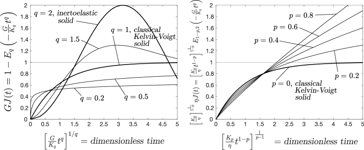
Figure 7: Left: Normalized creep compliance, $GJ(t)$, of the spring – Scott-Blair element in parallel for values $q=$ 0.2, 0.5, 1, 1.5 and 2 as a function of the dimensionless time $\Big{[}\frac{G}{K_{q}}$$t^{q}$$\Big{]}^{\nicefrac{{\text{1}}}{{q}}}$. Right: Normalized creep compliance, $\left[\frac{K_{p}}{\eta}\right]^{\frac{\text{1}}{\text{1}-p}}$$\eta J(t)$, of the springpot – dashpot element in parallel for values of $p=$ 0, 0.2, 0.4, 0.6 and 0.8 as a function of the dimensionless time $\Big{[}\frac{K_{p}}{\eta}$$t^{\text{1}-p}$$\Big{]}^{\frac{\text{1}}{\text{1}-p}}$.

Special Cases: 1. Spring – Scott-Blair element in parallel $(p=\text{0}$, $q\in\mathbb{R}^{+}\text{, }K_{p}=G)$

$$\psi(t)= \frac{\text{1}}{K_{q}}\frac{\mathrm{d}}{\mathrm{d}t}\left[\frac{\text{1}}{t^{\text{1}-q}}E_{q\text{, }q}\left(-\frac{G}{K_{q}}t^{q}\right)\right]=$$ (122)

$$\frac{\text{1}}{K_{q}}t^{q-\text{2}}E_{q\text{, }q-\text{1}}\left(-\frac{G}{K_{q}}t^{q}\right)$$

Again the right-hand side of Eq. (122) is valid for $q>$ 1. For the case when 0 $\leq q\leq$ 1 (spring – springpot in parallel) we use Eq. (120) with $p=$ 0

$$\psi(t)= \frac{\text{1}}{K_{q}}\Bigg{[}\frac{\mathrm{d}^{\text{1}-q}}{\mathrm{d}t^{\text{1}-q}}\delta(t-\text{0})-$$ (123)

$$\frac{G}{K_{q}}\frac{\text{1}}{t^{\text{2}-\text{2}q}}E_{q\text{, }\text{2}q-\text{1}}\left(-\frac{G}{K_{q}}t^{q}\right)\Bigg{]}$$

In the event that $q\leq$ 0.5 $(\text{2}q-\text{1}\leq\text{0})$, the expression for $\psi(t)$ offered by Eq. (121) needs to be used with $p=$ 0.

2. Springpot – Dashpot in parallel $(q=\text{1}$, $K_{q}=\eta$, $\text{0}\leq p\leq\text{1})$. In this case we need to use directly Eq. (120) with $p=$ 1

$$\psi(t)=\frac{\text{1}}{\eta}\left[\delta(t-\text{0})-\frac{K_{p}}{\eta}\frac{\text{1}}{t^{p}}E_{\text{1}-p\text{, }\text{1}-p}\left(-\frac{K_{p}}{\eta}t^{\text{1}-p}\right)\right]$$ (124)

The complex creep function, $\mathcal{C}(\omega)$, of the generalized fractional Kelvin-Voigt element derives directly from Eq. (103) gives that $\mathcal{C}(s)=$ $\nicefrac{{\mathcal{J}(s)}}{{s}}$

$$\mathcal{C}(s)=\frac{\gamma(s)}{\accentset{\mbox{\large.}}{\tau}(s)}=\frac{\text{1}}{K_{q}}\frac{\text{1}}{s^{\text{1}+p}(s^{r}+\frac{K_{p}}{K_{q}})}\text{,}\enskip\text{with}\enskip p\text{, }r\in\mathbb{R}^{+}$$ (125)

and $r=q-p>\text{0}$.

The inverse Laplace transform of Eq. (125) is evaluated with the convolution integral given by Eq. (68) where

$$f(t)= \mathcal{L}^{-\text{1}}\left\{\mathcal{F}(s)\right\}=\mathcal{L}^{-\text{1}}\left\{\frac{\text{1}}{K_{q}}\frac{\text{1}}{s^{\text{1}+p}}\right\}=$$ (126)

$$\frac{\text{1}}{K_{q}}\frac{\text{1}}{\Gamma(\text{1}+p)}t^{p}\text{,}\enskip p\in\mathbb{R}^{+}$$

and $h(t)=\mathcal{L}^{-\text{1}}\left\{\mathcal{H}(s)\right\}$ is given by Eq. (70). Substitution of the results of Eqs. (126) and (70) into the convolution integral given by Eq. (68), the creep compliance, $J(t)$, of the generalized fractional Kelvin-Voigt element is

$$J(t)= \mathcal{L}^{-\text{1}}\left\{\mathcal{C}(s)\right\}=$$ (127)

$$\frac{\text{1}}{K_{q}}\frac{\text{1}}{\Gamma(\text{1}+p)}\int_{\text{0}}^{t}(t-\xi)^{p}\xi^{r-\text{1}}E_{r\text{, }r}\left(-\frac{K_{p}}{K_{q}}\xi^{r}\right)\mathrm{d}\xi$$

which is the fractional integral of orde $\text{1}+p$ of the function given by Eq. (70) in which $r=q-p$

$$J(t)= \frac{\text{1}}{K_{q}}I^{\text{1}+p}\left[\frac{\text{1}}{t^{\text{1}-q+p}}E_{q-p\text{, }q-p}\left(-\frac{K_{p}}{K_{q}}t^{q-p}\right)\right]=$$ (128)

$$\frac{\text{1}}{K_{q}}t^{q}E_{q-p\text{, }q+\text{1}}\left(-\frac{K_{p}}{K_{q}}t^{q-p}\right)\text{,}\enskip\text{0}<q<p\in\mathbb{R}^{+}$$

where the right-hand side of Eq. (128) was evaluated by using the general result offered by Eq. (58) with $\alpha=\beta=q-p$. The result of Eq. (128) has been presented by Schiessel et al. (1995); Hristov (2019).

Table 4: Frequency-response functions and the corresponding causal time-response functions of the generalized fractional derivative Kelvin-Voigt element and of its special cases.

	Generalized Fractional Derivative Kelvin-Voigt Element	Spring – Scott-Blair Parallel Connection	Springpot – Dashpot Parallel Connection
Constitutive Equation	$\tau(t)=K_{p}\cfrac{\mathrm{d}^{p}\gamma(t)}{\mathrm{d}t^{p}}+K_{q}\cfrac{\mathrm{d}^{q}\gamma(t)}{\mathrm{d}t^{q}}$	$\tau(t)=G\gamma(t)+K_{q}\cfrac{\mathrm{d}^{q}\gamma(t)}{\mathrm{d}t^{q}}$	$\tau(t)=K_{q}\cfrac{\mathrm{d}^{q}\gamma(t)}{\mathrm{d}t^{q}}+\eta\cfrac{\mathrm{d}\gamma(t)}{\mathrm{d}t}$
Complex Dynamic Modulus $\mathcal{G}(\omega)=\cfrac{\tau(\omega)}{\gamma(\omega)}$	$K_{p}(\operatorname{i}\omega)^{p}+K_{q}(\operatorname{i}\omega)^{q}$	$G+K_{q}(\operatorname{i}\omega)^{q}$	$K_{q}(\operatorname{i}\omega)^{q}+\eta\operatorname{i}\omega$
Complex Dynamic Viscosity $\mathcal{\eta}(\omega)=\frac{\tau(\omega)}{\accentset{\mbox{\large.}}{\gamma}(\omega)}$	$\cfrac{K_{p}(\operatorname{i}\omega)^{p}+K_{q}(\operatorname{i}\omega)^{q}}{\operatorname{i}\omega}$	$G\left[\pi\delta(\omega-\text{0})-\operatorname{i}\cfrac{\text{1}}{\omega}\right]+K_{q}\cfrac{\text{1}}{(\operatorname{i}\omega)^{\text{1}-q}}$	$\eta+K_{q}\cfrac{\text{1}}{(\operatorname{i}\omega)^{\text{1}-q}}$
Complex Dynamic Compliance $\mathcal{J}(\omega)=\frac{\text{1}}{\mathcal{G}(\omega)}=\frac{\gamma(\omega)}{\tau(\omega)}$	$\cfrac{\text{1}}{K_{p}(\operatorname{i}\omega)^{p}+K_{q}(\operatorname{i}\omega)^{q}}$	$\cfrac{\text{1}}{G+K_{q}(\operatorname{i}\omega)^{q}}$	$\cfrac{\text{1}}{\eta}\cfrac{\eta\big{/}K_{q}}{\operatorname{i}\omega\left[(\operatorname{i}\omega)^{-\text{1}+q}+\frac{\eta}{K_{q}}\right]}$
Complex Creep Function $\mathcal{C}(\omega)=\frac{\gamma(\omega)}{\accentset{\mbox{\large.}}{\tau}(\omega)}$	$\cfrac{\text{1}}{K_{p}(\operatorname{i}\omega)^{p+\text{1}}+K_{q}(\operatorname{i}\omega)^{q+\text{1}}}$	$\cfrac{\text{1}}{\operatorname{i}\omega\left[G+K_{q}(\operatorname{i}\omega)^{q}\right]}$	$\cfrac{\text{1}}{\eta}\cfrac{\eta\big{/}K_{q}}{\operatorname{i}\omega\left[(\operatorname{i}\omega)^{q}+\frac{\eta}{K_{q}}\operatorname{i}\omega\right]}$
Complex Dynamic Fluidity $\mathcal{\phi}(\omega)=\frac{\text{1}}{\eta(\omega)}=\frac{\accentset{\mbox{\large.}}{\gamma}(\omega)}{\tau(\omega)}$	$\cfrac{\operatorname{i}\omega}{K_{p}(\operatorname{i}\omega)^{p}+K_{q}(\operatorname{i}\omega)^{q}}$	$\cfrac{\operatorname{i}\omega}{G+K_{q}(\operatorname{i}\omega)^{q}}$	$\cfrac{\text{1}}{\eta}\cfrac{(\operatorname{i}\omega)^{\text{1}-q}}{(\operatorname{i}\omega)^{\text{1}-q}+\frac{K_{q}}{\eta}}$
Memory Function $M(t)$	$\left[\cfrac{K_{p}}{\Gamma(-p)}\cfrac{\text{1}}{t^{p+\text{1}}}+\cfrac{K_{q}}{\Gamma(-q)}\cfrac{\text{1}}{t^{q+\text{1}}}\right]U(t-\text{0})$	$G\delta(t-\text{0})+\cfrac{K_{q}}{\Gamma(-q)}\cfrac{\text{1}}{t^{q+1}}U(t-\text{0})$	$\cfrac{K_{q}}{\Gamma(-q)}\cfrac{\text{1}}{t^{q+\text{1}}}U(t-\text{0})+\eta\cfrac{\mathrm{d}\delta(t-\text{0})}{\mathrm{d}t}$
Relaxation Modulus $G(t)$	$\left[\cfrac{K_{p}}{\Gamma(\text{1}-p)}\cfrac{\text{1}}{t^{p}}+\cfrac{K_{q}}{\Gamma(\text{1}-q)}\cfrac{\text{1}}{t^{q}}\right]U(t-\text{0})$	$\left[G+\cfrac{K_{q}}{\Gamma(\text{1}-q)}\cfrac{\text{1}}{t^{q}}\right]U(t-\text{0})$	$\cfrac{K_{q}}{\Gamma(\text{1}-q)}\cfrac{\text{1}}{t^{q}}U(t-\text{0})+\eta\delta(t-\text{0})$
Impulse Fluidity $\phi(t)$	$\cfrac{\text{1}}{K_{q}}\cfrac{\text{1}}{t^{\text{1}-q}}E_{q-p\text{, }q}\left(-\cfrac{K_{p}}{K_{q}}t^{q-p}\right)$	$\cfrac{\text{1}}{K_{q}}\cfrac{\text{1}}{t^{\text{1}-q}}E_{q\text{, }q}\left(-\cfrac{G}{K_{q}}t^{q}\right)$	$\cfrac{\text{1}}{\eta}\left[E_{\text{1}-q}\left(-\cfrac{K_{q}}{\eta}\,t^{\text{1}-q}\right)\right]$ 0 $\leq q\leq$ 1 or $\cfrac{\text{1}}{\eta}\left[\text{1}-E_{q-\text{1}}\left(-\cfrac{\eta}{K_{q}}\,t^{q-\text{1}}\right)\right]$ 1 $\leq q\in\mathbb{R}^{+}$
Creep Compliance $J(t)$	$\cfrac{\text{1}}{K_{q}}t^{q}E_{q-p\text{, }q+\text{1}}\left(-\cfrac{K_{p}}{K_{q}}t^{q-p}\right)$	$\cfrac{\text{1}}{G}\left[U(t-\text{0})-E_{q}\left(-\cfrac{G}{K_{q}}t^{q}\right)\right]$	$\cfrac{\text{1}}{\eta}tE_{\text{1}-q\text{, 2}}\left(-\cfrac{K_{q}}{\eta}t^{\text{1}-q}\right)$
Impulse Strain-rate Response Function $\psi(t)$	$\cfrac{\text{1}}{K_{q}}\cfrac{\text{1}}{t^{\text{2}-q}}\Bigg{[}\cfrac{\text{1}}{\Gamma(-\text{1}+q)}\,U(t-\text{0})-\quad\quad\quad$ $\quad\quad\quad\cfrac{K_{p}}{K_{q}}\cfrac{\text{1}}{t^{p-q}}E_{q-p\text{, }\text{2}q-p-\text{1}}\left(-\cfrac{K_{p}}{K_{q}}t^{q-p}\right)\Bigg{]}$	$\cfrac{\text{1}}{K_{q}}\cfrac{\text{1}}{t^{\text{2}-q}}\Bigg{[}\cfrac{\text{1}}{\Gamma(-\text{1}+q)}\,U(t-\text{0})-\quad$ $\quad\cfrac{G}{K_{q}}\cfrac{\text{1}}{t^{-q}}E_{q\text{, }\text{2}q-\text{1}}\left(-\cfrac{G}{K_{q}}t^{q}\right)\Bigg{]}$	$\cfrac{\text{1}}{\eta}\Bigg{[}\delta(t-\text{0})-\cfrac{K_{q}}{\eta}\cfrac{\text{1}}{t^{q}}E_{\text{1}-q\text{, }\text{1}-q}\left(-\cfrac{K_{q}}{\eta}t^{\text{1}-q}\right)\Bigg{]}$

Special Cases: 1. Spring – Scott-Blair element in parallel $(p=\text{0}$, $K_{p}=G\text{, }q\in\mathbb{R}^{+})$. In this case where $p=\text{0}$, Eq. (128) gives

$$J(t)=\frac{\text{1}}{K_{q}}t^{q}E_{q\text{, }q+\text{1}}\left(-\frac{G}{K_{q}}t^{q}\right)$$ (129)

Alternatively, the creep compliance, $J(t)$, for $p=$ 0 can be evaluated by returning to the expression of the complex creep function, $\mathcal{C}(s)$, of the generalized fractional Kelvin-Voigt element given by Eq. (125) by examining the special case where $r=q-p=q$

$$\mathcal{C}(s)=\frac{\text{1}}{K_{q}}\frac{\text{1}}{s(s^{q}+\frac{G}{K_{q}})}=\frac{\text{1}}{G}\frac{\frac{G}{K_{q}}}{s(s^{q}+\frac{G}{K_{q}})}$$ (130)

The inverse Laplace transform of the right-hand side of Eq. (130) is known

$$J(t)= \mathcal{L}^{-\text{1}}\left\{\mathcal{C}(s)\right\}=\mathcal{L}^{-\text{1}}\left\{\frac{\text{1}}{G}\frac{\frac{G}{K_{q}}}{s(s^{q}+\frac{G}{K_{q}})}\right\}=$$ (131)

$$\frac{\text{1}}{G}\left[\text{1}-E_{q}\left(-\frac{G}{K_{q}}t^{q}\right)\right]\text{, }q\in\mathbb{R}^{+}$$

The result of Eq. (131) has been presented by Koeller (1984); Schiessel et al. (1995) in their studies in viscoelasticity and by Westerlund and Ekstam (1994) for a capacitor model of mixed dielectrics. By employing the recurrence relation (57) of the Mittag-Leffler function

$$E_{q}\left(-\frac{G}{K_{q}}t^{q}\right)= E_{q\text{, 1}}\left(-\frac{G}{K_{q}}t^{q}\right)=$$ (132)

$$\text{1}-\frac{G}{K_{q}}t^{q}E_{q\text{, }q+\text{1}}\left(-\frac{G}{K_{q}}t^{q}\right)$$

the substitution of the right-hand side of Eq. (132) into the right-hand side of Eq. (131) yields the expression offered by Eq. (129); therefore the result offered by Eq. (129) (outcome of the fractional integral) and the result offered by Eq. (131) (inverse Laplace transform of the complex creep function) are identical. Figure 7 (left) plots the normalized creep compliance (retardation function) of the spring – Scott-Blair element parallel connection, $GJ(t)$, for values of $q=$ 0.2, 0.5, 1, 1.5 and 2 as a function of the dimensionless time $\Big{[}\frac{G}{K_{q}}$$t^{q}$$\Big{]}^{\nicefrac{{\text{1}}}{{q}}}$. When $q=$ 2 (inertoelastic solid), the creep compliance, $J(t)$, exhibits oscillatory behavior since the spring and the inerter exchange their potential (spring) and kinetic (inerter) energies.

2. Springpot – Dashpot in parallel $(q=\text{1}$, $K_{q}=\eta$, $\text{0}<p<\text{1})$. In this case where $q=\text{1}$ and $K_{q}=K_{\text{1}}=\eta$, Eq. (128) yields

$$J(t)=\frac{\text{1}}{\eta}tE_{\text{1}-p\text{, }\text{2}}\left(-\frac{K_{p}}{\eta}t^{\text{1}-p}\right)$$ (133)

For the limit case where $p=$ 0 and $K_{p}=K_{\text{0}}=G$, Eq. (133) yields $J(t)=\frac{\text{1}}{\eta}tE_{\text{1, 2}}$$\Big{(}-\frac{G}{\eta}$$t$ $\Big{)}$. Using the identity that $E_{\text{1, 2}}(z)=$ $\frac{e^{z}-\text{1}}{z}$, together with $\nicefrac{{\eta}}{{G}}=$ $\lambda=$ relaxation time, $J(t)=$ $\frac{\text{1}}{G}\Big{[}$$U(t-\text{0})-e$${}^{-\nicefrac{{t}}{{\lambda}}}\Big{]}$, which is the creep compliance of the classical Kelvin-Voigt solid. Figure 7 (right) plots the normalized creep compliance of the springpot – dashpot parallel connection, $\left[\frac{K_{p}}{\eta}\right]^{\frac{\text{1}}{\text{1}-p}}$$\eta J(t)$, for various values of $p$.

The five causal time-response functions of the generalized fractional Kelvin-Voigt element together with the time-response functions for the special cases of the spring – Scott-Blair element parallel connection $(p=\text{0})$, and the springpot – dashpot parallel connection $(q=\text{1})$ are summarized in Table 4.

8 Conclusions

In this paper we studied the five time-response functions of the generalized fractional derivative Maxwell fluid and the generalized fractional derivative Kelvin-Voigt element. These two rheological models are in-series or parallel connections of two Scott-Blair elements which are the elementary fractional derivative elements. In this work the order of differentiation in each Scott-Blair element is allowed to exceed unity reaching values up to 2; and at this limit case the Scott-Blair element becomes an inerter. With this generalization, where the Scott-Blair element goes beyond the traditional springpot, inertia effects may be captured in addition to the monotonic viscoelastic effects. In the special case of spring – inerter connections, the time response functions which are not superpositions exhibit oscillatory behavior given the continuous exchange of potential energy (spring) and kinetic energy (inerter).

In addition to the well studied relaxation moduli and creep compliances of the two generalized fractional derivative rheological models, we compute closed-form expressions of the remaining three time-response functions which are the memory function, the impulse fluidity (impulse response function) and the impulse strain-rate response function. Central role to these calculations plays the fractional derivative of the Dirac delta function which is merely the kernel appearing in the convolution of the Riemann-Liouville definition of the fractional derivative of a function and it is the generalization of the Gel’fand and Shilov (1964) definition of the Dirac delta function and its integer-order derivatives for any positive real number. This finding shows that the fractional derivative of the Dirac delta function, $\frac{\mathrm{d}^{q}\delta(t-\text{0})}{\mathrm{d}t^{q}}$, is finite everywhere other than at the singularity point and it is the inverse Fourier transform of $(\operatorname{i}\omega)^{q}$ where $q$ is any positive real number. The fractional derivative of the Dirac delta function emerges as key function in the derivation of the time-response functions of generalized fractional derivative rheological models, since it makes possible the extraction of the singularities embedded in the fractional derivatives of the two-parameter Mittag-Leffler function that emerges invariably in the time-response functions of fractional derivative rheological models. The mathematical techniques developed in this work can be applied to calculate the time-response function of higher-parameter rheological models that involve fractional-order time derivatives.

Conflict of interest The authors declare that they have no conflict of interest.

Funding Not applicable.

References

- Atakhorrami et al. (2008) Atakhorrami M, Mizuno D, Koenderink G, Liverpool TB, MacKintosh FC, Schmidt CF (2008) Short-time inertial response of viscoelastic fluids measured with Brownian motion and with active probes. Physical Review E 77(6):061508
- Atanackovic et al. (2015) Atanackovic TM, Janev M, Oparnica L, Pilipovic S, Zorica D (2015) Space–time fractional Zener wave equation. Proceedings of the Royal Society A: Mathematical, Physical and Engineering Sciences 471(2174):20140614
- Bagley and Torvik (1983a) Bagley RL, Torvik PJ (1983a) Fractional calculus - A different approach to the analysis of viscoelastically damped structures. AIAA Journal 21(5):741–748
- Bagley and Torvik (1983b) Bagley RL, Torvik PJ (1983b) A theoretical basis for the application of fractional calculus to viscoelasticity. Journal of Rheology 27(3):201–210
- Bird et al. (1987) Bird RB, Armstrong RC, Hassager O (1987) Dynamics of polymeric liquids. Vol. 1: Fluid mechanics, 2nd edn. Wiley, New York, NY
- Bode (1945) Bode HW (1945) Network analysis and feedback amplifier design. van Nostrand New York
- Bracewell (1965) Bracewell RN (1965) The Fourier transform and its applications. McGraw-Hill Inc., New York, NY
- Caputo and Mainardi (1971) Caputo M, Mainardi F (1971) A new dissipation model based on memory mechanism. Pure and Applied Geophysics 91(1):134–147
- Challamel et al. (2013) Challamel N, Zorica D, Atanacković TM, Spasić DT (2013) On the fractional generalization of eringen’s nonlocal elasticity for wave propagation. Comptes Rendus Mécanique 341(3):298–303
- Clough and Penzien (1970) Clough RW, Penzien J (1970) Dynamics of structures. McGraw-Hill, New York, NY
- Craiem and Magin (2010) Craiem D, Magin RL (2010) Fractional order models of viscoelasticity as an alternative in the analysis of red blood cell (RBC) membrane mechanics. Physical Biology 7(1):013001
- Djordjević et al. (2003) Djordjević VD, Jarić J, Fabry B, Fredberg JJ, Stamenović D (2003) Fractional derivatives embody essential features of cell rheological behavior. Annals of Biomedical Engineering 31(6):692–699
- Domínguez-García et al. (2014) Domínguez-García P, Cardinaux F, Bertseva E, Forró L, Scheffold F, Jeney S (2014) Accounting for inertia effects to access the high-frequency microrheology of viscoelastic fluids. Physical Review E 90(6):060301
- Erdélyi (1953) Erdélyi A (ed) (1953) Bateman Manuscript Project, Higher Transcendental Functions Vol III. McGraw-Hill, New York, NY
- Erdélyi (1954) Erdélyi A (ed) (1954) Bateman Manuscript Project, Tables of Integral Transforms Vol I. McGraw-Hill, New York, NY
- Evans et al. (2009) Evans RML, Tassieri M, Auhl D, Waigh TA (2009) Direct conversion of rheological compliance measurements into storage and loss moduli. Physical Review E 80(1):012501
- Ferry (1980) Ferry JD (1980) Viscoelastic properties of polymers. John Wiley & Sons, New York, NY
- Friedrich (1991) Friedrich CHR (1991) Relaxation and retardation functions of the Maxwell model with fractional derivatives. Rheologica Acta 30(2):151–158
- Gel’fand and Shilov (1964) Gel’fand IM, Shilov GE (1964) Generalized functions, Vol. 1 Properties and operations. AMS Chelsea Publishing: An Imprint of the American Mathematical Society, Providence, RI
- Gemant (1936) Gemant A (1936) A method of analyzing experimental results obtained from elastoviscous bodies. Physics 7(8):311–317
- Gemant (1938) Gemant A (1938) XLV. On fractional differentials. The London, Edinburgh, and Dublin Philosophical Magazine and Journal of Science 25(168):540–549
- Giesekus (1995) Giesekus H (1995) An alternative approach to the linear theory of viscoelasticity and some characteristic effects being distinctive of the type of material. Rheologica Acta 34(1):2–11
- Gittes and MacKintosh (1998) Gittes F, MacKintosh FC (1998) Dynamic shear modulus of a semiflexible polymer network. Physical Review E 58(2):R1241
- Glöckle and Nonnenmacher (1991) Glöckle WG, Nonnenmacher TF (1991) Fractional integral operators and Fox functions in the theory of viscoelasticity. Macromolecules 24(24):6426–6434
- Glöckle and Nonnenmacher (1993) Glöckle WG, Nonnenmacher TF (1993) Fox function representation of non-Debye relaxation processes. Journal of Statistical Physics 71(3-4):741–757
- Glöckle and Nonnenmacher (1994) Glöckle WG, Nonnenmacher TF (1994) Fractional relaxation and the time-temperature superposition principle. Rheologica Acta 33(4):337–343
- Gorenflo and Mainardi (1997) Gorenflo R, Mainardi F (1997) Fractional calculus. In: Fractals and fractional calculus in continuum mechanics, Springer, pp 223–276
- Gorenflo et al. (2014) Gorenflo R, Kilbas AA, Mainardi F, Rogosin SV, et al. (2014) Mittag-Leffler functions, related topics and applications Vol. 2. Springer
- Harris and Crede (1976) Harris CM, Crede CE (1976) Shock and vibration handbook, 2nd edn. McGraw-Hill, New York, NY
- Haubold et al. (2011) Haubold HJ, Mathai AM, Saxena RK (2011) Mittag-Leffler functions and their applications. Journal of Applied Mathematics 2011
- Heymans and Bauwens (1994) Heymans N, Bauwens JC (1994) Fractal rheological models and fractional differential equations for viscoelastic behavior. Rheologica Acta 33(3):210–219
- Hristov (2019) Hristov J (2019) Response functions in linear viscoelastic constitutive equations and related fractional operators. Mathematical Modelling of Natural Phenomena 14(3):305
- Indei et al. (2012) Indei T, Schieber JD, Córdoba A (2012) Competing effects of particle and medium inertia on particle diffusion in viscoelastic materials, and their ramifications for passive microrheology. Physical Review E 85(4):041504
- Jaishankar and McKinley (2013) Jaishankar A, McKinley GH (2013) Power-law rheology in the bulk and at the interface: quasi-properties and fractional constitutive equations. Proceedings of the Royal Society A: Mathematical, Physical and Engineering Sciences 469(2149):20120284
- Koeller (1984) Koeller RC (1984) Applications of fractional calculus to the theory of viscoelasticity. Journal of Applied Mechanics 51(2):299–307
- Koh and Kelly (1990) Koh CG, Kelly JM (1990) Application of fractional derivatives to seismic analysis of base-isolated models. Earthquake Engineering & Structural Dynamics 19(2):229–241
- Le Page (1961) Le Page WR (1961) Complex variables and the Laplace transform for engineers. McGraw-Hill
- Lighthill (1958) Lighthill MJ (1958) An introduction to Fourier analysis and generalised functions. Cambridge University Press
- Lorenzo and Hartley (2002) Lorenzo CF, Hartley TT (2002) Variable order and distributed order fractional operators. Nonlinear Dynamics 29(1-4):57–98
- Mainardi (2010) Mainardi F (2010) Fractional calculus and waves in linear viscoelasticity: An introduction to mathematical models. Imperial College Press - World Scientific, London, UK
- Mainardi and Spada (2011) Mainardi F, Spada G (2011) Creep, relaxation and viscosity properties for basic fractional models in rheology. The European Physical Journal Special Topics 193(1):133–160
- Makris (1992) Makris N (1992) Theoretical and experimental investigation of viscous dampers in applications of seismic and vibration isolation. PhD thesis, State University of New York, Buffalo, NY
- Makris (1997a) Makris N (1997a) Three-dimensional constitutive viscoelastic laws with fractional order time derivatives. Journal of Rheology 41(5):1007–1020
- Makris (1997b) Makris N (1997b) Stiffness, flexibility, impedance, mobility, and hidden delta function. Journal of Engineering Mechanics 123(11):1202–1208
- Makris (2017) Makris N (2017) Basic response functions of simple inertoelastic and inertoviscous models. Journal of Engineering Mechanics 143(11):04017123
- Makris (2018) Makris N (2018) Time-response functions of mechanical networks with inerters and causality. Meccanica 53(9):2237–2255
- Makris (2019) Makris N (2019) The frequency response function of the creep compliance. Meccanica 54(1-2):19–31
- Makris and Constantinou (1991) Makris N, Constantinou MC (1991) Fractional-derivative Maxwell model for viscous dampers. Journal of Structural Engineering 117(9):2708–2724
- Makris and Constantinou (1992) Makris N, Constantinou MC (1992) Spring-viscous damper systems for combined seismic and vibration isolation. Earthquake Engineering & Structural Dynamics 21(8):649–664
- Makris and Deoskar (1996) Makris N, Deoskar HS (1996) Prediction of observed response of base-isolated structure. Journal of Structural Engineering 122(5):485–493
- Makris and Kampas (2009) Makris N, Kampas G (2009) Analyticity and causality of the three-parameter rheological models. Rheologica Acta 48(7):815–825
- Makris and Moghimi (2018) Makris N, Moghimi G (2018) Displacements and forces in structures with inerters when subjected to earthquakes. Journal of Structural Engineering 145(2):04018260
- Mason (2000) Mason TG (2000) Estimating the viscoelastic moduli of complex fluids using the generalized Stokes–Einstein equation. Rheologica Acta 39(4):371–78
- Mason and Weitz (1995) Mason TG, Weitz DA (1995) Optical measurements of frequency-dependent linear viscoelastic moduli of complex fluids. Physical Review Letters 74(7):1250
- Mason et al. (1997) Mason TG, Ganesan K, Van Zanten JH, Wirtz D, Kuo SC (1997) Particle tracking microrheology of complex fluids. Physical Review Letters 79(17):3282
- Miller and Ross (1993) Miller KS, Ross B (1993) An introduction to the fractional calculus and fractional differential equations. Wiley, New York, NY
- Nutting (1921) Nutting PG (1921) A study of elastic viscous deformation. Proceedings American Society for Testing Materials 21:1162–1171
- Oldham and Spanier (1974) Oldham K, Spanier J (1974) The Fractional Calculus. Mathematics in science and engineering, vol III. Academic Press Inc., San Diego, CA
- Palade et al. (1996) Palade LI, Verney V, Attané P (1996) A modified fractional model to describe the entire viscoelastic behavior of polybutadienes from flow to glassy regime. Rheologica Acta 35(3):265–273
- Papageorgiou and Smith (2005) Papageorgiou C, Smith MC (2005) Laboratory experimental testing of inerters. In: Proceedings of the 44th IEEE Conference on Decision and Control, IEEE, pp 3351–3356
- Papoulis (1962) Papoulis A (1962) The Fourier integral and its applications. McGraw-Hill Inc., New York, NY
- Pipkin (1986) Pipkin AC (1986) Lectures on Viscoelasticity Theory, vol 7, 2nd edn. Springer-Verlag New York Inc.
- Podlubny (1998) Podlubny I (1998) Fractional differential equations: An introduction to fractional derivatives, fractional differential equations, to methods of their solution and some of their applications. Elsevier
- Puig-de-Morales-Marinkovic et al. (2007) Puig-de-Morales-Marinkovic M, Turner KT, Butler JP, Fredberg JJ, Suresh S (2007) Viscoelasticity of the human red blood cell. American Journal of Physiology-Cell Physiology 293(2):C597–C605
- Rabotnov (1980) Rabotnov YN (1980) Elements of hereditary solid mechanics. MIR Publishers
- Reid (1983) Reid GJ (1983) Linear systems fundamentals. Continuous and discrete, classic and modern. McGraw-Hill Series in Electrical Engineering
- Riesz et al. (1949) Riesz M, et al. (1949) L’intégrale de Riemann-Liouville et le problème de Cauchy. Acta Mathematica 81:1–222
- Samko et al. (1974) Samko SG, Kilbas AA, Marichev OI (1974) Fractional Integrals and Derivatives; Theory and Applications, vol 1. Gordon and Breach Science Publishers, Amsterdam
- Schiessel et al. (1995) Schiessel H, Metzler R, Blumen A, Nonnenmacher TF (1995) Generalized viscoelastic models: Their fractional equations with solutions. Journal of Physics A: Mathematical and General 28(23):6567
- Scott Blair (1944) Scott Blair GW (1944) A survey of general and applied rheology. Isaac Pitman & Sons
- Scott Blair (1947) Scott Blair GW (1947) The role of psychophysics in rheology. Journal of Colloid Science 2(1):21–32
- Scott Blair and Caffyn (1949) Scott Blair GW, Caffyn JE (1949) VI. An application of the theory of quasi-properties to the treatment of anomalous strain-stress relations. The London, Edinburgh, and Dublin Philosophical Magazine and Journal of Science 40(300):80–94
- Scott Blair et al. (1947) Scott Blair GW, Veinoglou BC, Caffyn JE (1947) Limitations of the Newtonian time scale in relation to non-equilibrium rheological states and a theory of quasi-properties. Proceedings of the Royal Society of London Series A Mathematical and Physical Sciences 189(1016):69–87
- Smit and De Vries (1970) Smit W, De Vries H (1970) Rheological models containing fractional derivatives. Rheologica Acta 9(4):525–534
- Smith (2002) Smith MC (2002) Synthesis of mechanical networks: the inerter. IEEE Transactions on Automatic Control 47(10):1648–1662
- Suki et al. (1994) Suki B, Barabasi AL, Lutchen KR (1994) Lung tissue viscoelasticity: A mathematical framework and its molecular basis. Journal of Applied Physiology 76(6):2749–2759
- Triverio et al. (2007) Triverio P, Grivet-Talocia S, Nakhla MS, Canavero FG, Achar R (2007) Stability, causality, and passivity in electrical interconnect models. IEEE Transactions on Advanced Packaging 30(4):795–808
- Tschoegl (1989) Tschoegl NW (1989) The phenomenological theory of linear viscoelastic behavior: An introduction. Springer, Berlin, Heidelberg
- Veletsos and Verbic (1974) Veletsos AS, Verbic B (1974) Basic response functions for elastic foundations. Journal of Engineering Mechanics 100
- Westerlund and Ekstam (1994) Westerlund S, Ekstam L (1994) Capacitor theory. IEEE Transactions on Dielectrics and Electrical Insulation 1(5):826–839
- Zhu et al. (2015) Zhu S, Cai C, Spanos PD (2015) A nonlinear and fractional derivative viscoelastic model for rail pads in the dynamic analysis of coupled vehicle–slab track systems. Journal of Sound and Vibration 335:304–320