Precursors of the El Niño Phenomenon: A climate network analysis

Abstract

The identification of precursors of climatic phenomena has enormous practical importance. Recent work constructs a climate network based on surface air temperature data to analyze the El Niño phenomena. We utilize microtransitions which occur before the discontinuous percolation transition in the network as well as other network quantities to identify a set of reliable precursors of El Niño episodes. These precursors identify nine out of twelve El Niño episodes occurring in the period of $1979$ to $2018$ with a lead time varying from six to ten months. We also find indicators of tipping events in the data.

The climate system is highly complex nonlinear dynamical system consisting of various subsystems such as the atmosphere, the ocean, the cryosphere, the biosphere, and the lithosphere. The nonlinear interactions within these subsystems lead to various climatic phenomena on multiple timescales such as cyclones, the monsoon and oceanic currentscn2 . Climatic phenomena have major consequences for ecological and economic events. Hence the prediction of climatic phenomena is of enormous practical utility, but is quite difficult due to the complex and nonlinear nature of the phenomena under consideration. Thus, the construction of reliable predictors of such events is useful and important. Recent methods proposed to analyze such complex climate systems include the construction of a complex network from climate data cn1 ; cn2 ; tsr . These networks have been used to forecast some important climate phenomena, such as the monsoon monsoon1 ; monsoon2 , the North Atlantic Oscillation and El Niño events ygh -prl5 .

These climate networks are constructed using massive datasets consisting of the time series of weather observations at different geographic locations. Generally, the nodes are chosen to be geographic locations, and links are added based on the similarities between the dynamics at pairs of nodes. Recently, the utility of designing generic tools that reliably track the structural changes in the network has been highlighted. Tracking these structural changes in the climate network of temperatures reveals severe response to climatic events such as El Niño events.

The El Niño Southern Oscillation (ENSO) is the most influential climate phenomenon on interannual time scales. It is marked by irregular warm (El Niño) and cold (La Niña) anomalies of sea surface temperatures (SST) from the long-term mean state. Events are defined as the consecutive overlapping of three-month periods of SST anomalies ($\geq+0.5\degree C$) for warm (El Niño) events and ($\leq-0.5\degree C$) for cold (La Niña) events in the Niño $3.4$ region (i.e., $5\degree N$-$5\degree S$, $120\degree$-$170\degree W$). The threshold is further broken down into Weak ($0.5\degree C$ - $0.9\degree C$ SST anomaly), Moderate ($1.0\degree C$ - $1.4\degree C$), Strong ($1.5\degree C$ - $1.9\degree C$) and Very Strong ($\geq 2.0\degree C$) events. This phenomenon triggers many disruptions around the globe causing disastrous flooding in countries like Peru and Ecuador as well as heavy droughts in large areas of South America, Indonesia, and Australia. It is plausibly also associated with severe winters in Europe, droughts in India, China, and Brazil, intense tropical cyclones in the Caribbean, and epidemic diseases occurring in various places nino ; ninobook . The ENSO phenomenon is currently tracked and quantified by the NINO $3.4$ index. Here, we use various datasets of the daily near surface ($1000$hPa) air temperature of ERA-Interim reanalysis (The European Centre for Medium-Range Weather Forecasts (ECMWF)) within the period $1979$-$2018$ to forecast the development of the El Niño well in advance ecmwf . Such an early forecast of the El Niño event can contribute to better disaster management planning and efficient distribution of resources well before the calamity.

Complex network systems, ranging from ecosystems to financial markets and the climate, can have tipping points at which a phase transition to a contrasting dynamical regime occurs. A variety of indicators, such as the order parameter, and the susceptibility, quantify the loss of resilience occurring generically when dynamical network systems approach transition point rep ; rev . The framework of percolation theory has been used to analyze the behavior of connected clusters in the network and predict the transition point per . Discontinuous percolation transitions have been observed in the climate network. We analyze these discontinuous percolation transitions and try to identify a set of early warning precursors to these transitions, and use them to predict the onset of El Niño activity. We note that our precursors are able to predict El Niño activity from six to ten months in advance. Our methods are quite reliable, and only lead to one false positive prediction in the analysis of 39 years of data. Our methods consist of the analysis of microtransitions that occur before the discontinuous percolation transition and the topological analysis of network quantities such as node degrees, link densities and link lengths.

The existence and predictive utility of microtransitions has been the focus of recent work in the context of percolation phenomena. These microtransitions appear before the percolation transition for both the continuous and discontinuous cases and accumulate at the transition point. These microtransitions are signalled by small jumps in the order parameter, i.e. the size of the maximal cluster, and peaks in the variance of the order parameter. In the case of the climate network, the actual transition point is the point at which a discontinuous percolation transition is seen, with the usual jump in the order parameter. Here, we use the microtransitions to predict critical thresholds at which the percolation transition can occur micro . The predicted threshold values are characteristic of the data of the period for which the network is constructed and can hence be used as generic early-warning indicators of the El Niño years. The variance in the order parameter, i.e. the susceptibility at the critical point can also be used to identify pre-El Niño years (which we will call indicator years) , and thereby predict the El Niño in the subsequent year. We note that the jump in the order parameter has been used earlier to identify pre-El Niño years 1 , but the susceptibility constitutes a stronger indicator. Additionally, we have carried out the topological analysis of the climate network of each year and have found that several distinct features such as the distribution of network links, the degrees of the network nodes in the El Niño basin differentiate clearly between El Niño years and indicator years. Thus, this entire collection of features i.e. the susceptibility, critical correlation value, maximum value of correlation strength and total number of links observed in the climate network can be used as a set of precursors of an upcoming El Niño event.

The climate network is constructed by the following method. We use daily near surface ($1000$hPa) air temperature datasets [$\tilde{T}^{y}(d)$] recorded at $1,15,680$ nodes whose geographical location is fixed by a pair of latitude and longitude values. The grid size of the network can be changed by altering the resolution of nodes such that every element in the grid covers the same area on the globe. Thus the total number of nodes on the equator is given by, $n_{0}=360^{\degree}/r_{0}$, where $r_{0}$ is the grid resolution, and the total number of nodes on $mr_{0}$ latitude is given by $n_{m}=n_{0}\cos(mr_{0})$ where $m\in[-90/r_{0},90/r_{0}]$. The total number of nodes in the climate network is then $N=\sum_{m=0}^{m=90/r_{0}}2n_{m}-n_{0}$. A geographical grid of $726$ nodes with $7.5\degree$ grid resolution is constructed and links are added between the two nodes by calculating the Pearson correlation function between their temperatures. The filtered daily near surface air temperature $T^{y}(d)$ and the cross-correlation function $C^{y}_{i,j}$ are defined as follows 1 ,

$$T^{y}(d) = \frac{\tilde{T}^{y}(d)-mean(\tilde{T}(d))}{std(\tilde{T}(d))}$$ (1)

$$C^{y}_{i,j}(\tau) = \frac{\langle T^{y}_{i}(d-\tau)T^{y}_{j}(d)\rangle-\langle T^{y}_{i}(d-\tau)\rangle\langle T^{y}_{j}(d)\rangle}{\sqrt{(T^{y}_{i}(d-\tau)-\langle T^{y}_{i}(d-\tau)\rangle)^{2}}.\sqrt{(T^{y}_{j}(d)-\langle T^{y}_{j}(d)\rangle)^{2}}}$$ (2)

Temperature datasets over $39$ years from 1979 to 2018 have been used to built a network for each year from January $1^{st}$ till $31^{st}$ December, and $\tau$ is the time lag between $0$ to $200$ days. For each year, the data for the previous year is also required on account of the time lag. The appropriate time lag and its impact is discussed in tau . Here ”$mean$” and ”$std$” are the mean and standard deviation of the temperature on day ‘$d$’ over all years. Only the temperature data points prior to day ‘$d$’ are considered. The averages ($\langle~{}~{}\rangle_{d}$) considered here are taken over $365$ days. The weight of the link between $i$ and $j$ is defined as the maximum of the cross-correlation function $max$($C^{y}_{i,j}(\tau)$). Here, links were added one by one with decreasing link strength, i.e. the links or edges with the highest weight (maximum of the cross-correlation function $C^{y}_{i,j}$), are added first to the network. Further edges are added in order by decreasing weight. Thus the network evolves as a function of $C$, as links of weights ranging from a given value of $C$ upto the maximum value of $C$ are added at each stage. Quantities such as the order parameter, which is the normalized size of the largest cluster ($s_{1}$) and the susceptibility ($\chi$) for each distinct value of $C$ are studied. These are defined by the relations 1 ,

$$s_{1} = \frac{S_{1}}{N}$$ (3)

$$\chi = \frac{\sum_{s}^{{}^{\prime}}s^{2}n_{s}(C)}{\sum_{s}^{{}^{\prime}}sn_{s}(C)}$$ (4)

Here, $S_{1}$ is the size of largest cluster and $N$ is the total number of nodes, $n_{s}(C)$ is the number of clusters of size ”$s$” for link’s weight $C$ and below, and the prime on the sums indicates the exclusion of the largest cluster $S_{1}$ in each measurement. The transition to the percolating state in this climate network is identified via the existence of a giant cluster containing $O(N)$ nodes. As mentioned earlier, this quantity is identified as the order parameter

We note that El Niño events have been classified as very strong, strong and moderate events based on the El Niño index as explained above, and compare the networks corresponding to each class. These networks are characterized by plotting the susceptibility ($\chi$) and the largest normalized cluster ($s_{1}$). A discontinuous phase transition is clearly observed in $s_{1}$ (the largest normalized cluster. We plot these quantities as functions of $C$ for typical years with El Niño events of each class, as well as the preceding years, which turn out to be indicator years of the event.

The year is indicated at the top of all the plots, and the red line marks the critical value $C_{c}$ on the $x$-axis at which the largest jump is observed in $s_{1}$. The transition to percolation is signaled by the value of $s_{1}$ tending toward one, and the existence of a maximal cluster. It can be clearly seen from the plots that $\Delta s_{1}$, the jump in the size of the maximal cluster, is largest for the indicator year i. e. one year prior to the El Niño episode. The susceptibility $\chi$ is also plotted on the same graphs. It can be seen that the magnitude of the jump $\Delta\chi$ is significantly larger in the indicator years, i.e. one year prior to the El Niño episodes compared to other years.

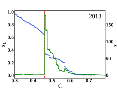
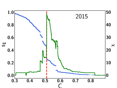
(a)	(d)
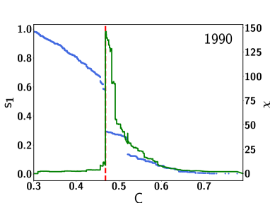
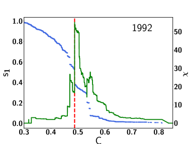
(b)	(e)
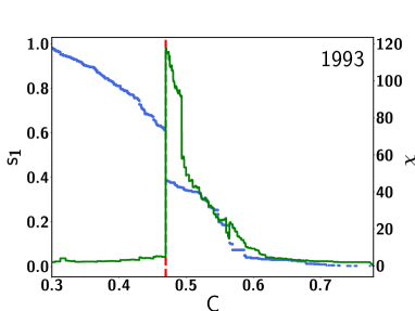
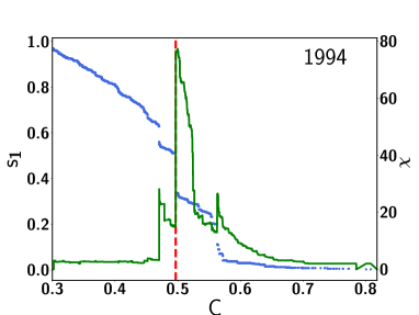
(c)	(f)

Figure 1: The largest cluster $s_{1}$ (blue dotted line) and susceptibility $\chi$ (green line) is plotted as a function of the link strength $C$ for the network. Plots (a)(December 2013), (b)(December 1990) (c ) December 1993, which are years which precede a very strong El Niño episode, strong El Niño episode, and a moderate El Niño episode, respectively. Plots (d) (e) (f) are for years when the El Niño episode peaks, (d) very strong El Niño episode, December 2015. (e) strong El Niño episode, December 1992. (f) moderate El Niño episode, December 1994.

The susceptibility of the network gives the measure of the change in the formation of clusters of varied sizes at a given correlation strength. We note that while the order parameter jump has been suggested as a measure of the precursor 1 , the susceptibility is a more definitive and reliable precursor for the upcoming El Niño episode as not only is the largest peak $\Delta\chi$ significant, but the peaks in the susceptibility before it also have a very distinct pattern. Ref.1 suggested that susceptibility has seemingly no distinct relation with the El Niño Index and hence refrained from using the susceptibility as a predictor. In contrast to their observations, it can be seen from the plots above that the susceptibility has a distinct pattern and clearly shows a series of small transitions i.e. microtransitions before the percolation transition point.

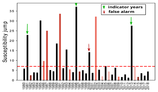
Figure 2: The maximum jump in the Susceptibility $\chi$ for each year ($1979$-$2018$). El Niño years are shown in red with a gradation according to their strength. There have been $12$ such El Niño episodes out of which ($1982$, $1997$ and $2015$) are very strong El Niño years, ($1987$ and $1991$) are strong El Niño years , ($1986$, $1994$, $2002$ and $2009$) are moderate El Niño years and ($2004$, $2006$ and $2014$) are weak El Niño years.

We adopt the following criterion for the prediction of the El Niño. When the maximum jump in the susceptibility crosses a threshold value ($7.1$) an El Niño episode is predicted in the following year. Using this threshold value, nine events are predicted correctly out of twelve with just one false alarm. Almost all the events (very strong, strong and moderate El Niño events) can be predicted by our criterion except for a few weak El Niño events. The threshold has been set to be the value of the jump of the year 2005, which is the indicator year for a weak El Niño year. This minimizes the false alarms. If our results are compared with the normalized largest cluster used as an indicator (as per Ref.1 ) , it is seen that when $\Delta s_{1}$ crosses a threshold value ($0.286$), an El Niño episode is predicted in the next year. It predicts eight events correctly out of twelve El Niño events with two false alarms.

The susceptibility pattern prior to an El Niño episode is further analyzed by looking at the microtransitions signaled by small jumps in the susceptibility occurring before the phase-transition signaled by the largest jump. The locations of these microtransitions, plotted as a function of $C_{i}$ can be used to predict the critical value of $C_{c}$ in the given year.

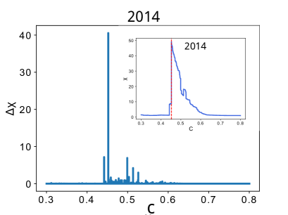
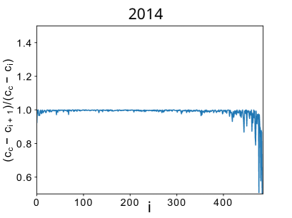
(a)	(b)

Figure 3: (a) The jump $\Delta\chi$ as a function of the link strength $C$. (Inset: The susceptibility $\chi$ as a function of the link strength $C$ for the network one year before a very strong El Niño episode, December 2014.) (b) The scaling relation for the relative $\Delta\chi$ positions, $\left(C_{c}-C_{i+1}/C_{c}-C_{i}\right)$ as a function of the index $i$.

The red line in the susceptibility plot indicates the value of the link strength $C_{c}$ at which the climate network undergoes the percolation transition i.e. the formation of a giant component (cluster) containing $O(N)$ nodes [Fig.3(Inset)]. In [Fig.3(a)] the magnitude of successive jumps in the susceptibility with respect to the link strength is plotted. Using the scaling relation plotted in [Fig.3(b)] one can write,

$$\frac{C_{c}-C_{i+1}}{C_{c}-C_{i}}=0.9956$$ (5)

This scaling relation enables us to predict the transition point at which the network undergoes a percolation transition. We analyze these microtransitions for each network for each year within the period $1979$-$2018$. It is noted that for the indicator year $2014$, $C_{c}=0.4669$ using the values $i=44,C_{44}=0.6719$ and $C_{45}=0.6710$. The value of $C_{c}$ from the scaling relation is in reasonable agreement with the actual value of $C_{c}=0.4522$ from the order parameter jump. A similar pattern of activity is observed for all the pre-El Niño years. One can predict the transition point using the above scaling relation and starting from $i\approx 45,C_{45}\approx 0.66$ for all the pre-El Niño years in this data. Thus a distinct pattern of microtransitions is observed before the percolation phase transition point for all the indicator years prior to an El Niño activity. We notice some crucial points regarding these microtransitions in the indicator years such as, the $C_{c}$ value ranges from $0.4411$ to $0.4736$ for all indicator years except for the indicator year $2008$ prior to moderate El Niño episode. Again, $|\Delta\chi|$ the jump in the susceptibility is very high ranging between $40$ to $100$ for indicator years compared to the other years. The topological analysis of all the $39$ climate networks has also been carried out and the histogram of the link lengths $\ell_{i,j}$ (i.e. the geographical distance between point $i$ and point $j$) observed in the network is plotted. These remote connections are typically of the order of thousands of kilometers and have been called teleconnections prl5 . Teleconnections are of great importance in climate dynamics as they reflect the underlying climatic currents mirroring the transportation of energy. These teleconnections between various remote regions have different weights associated with them. It can be seen that the number of large distance links increase substantially during El Niño and La Niña activity.

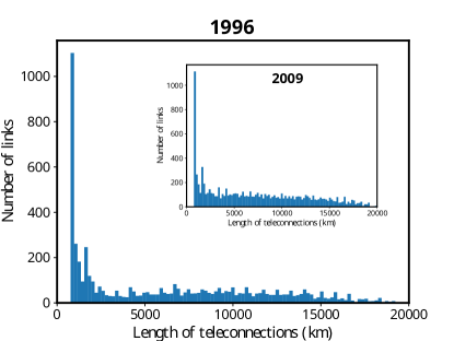
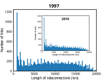
(a)	(b)

Figure 4: The histogram of the teleconnections in kilometers for the network (a) One year before a very strong El Niño episode, December 1996. (Inset: One year before strong La Niña episode, December 2009). (b) During a very strong El Niño episode, December 1997. (Inset: During a strong La Niña episode, December 2010).

The above figures indicate that the total number of teleconnections increase significantly during El Niño as well as La Niña activity. An increased number of teleconnections with higher value of correlation strength are also seen for El Niño years. The degrees of nodes (number of links per node) at each grid location has been plotted in Figure [5(c)] to analyze the geographical distribution of nodes of high degree.

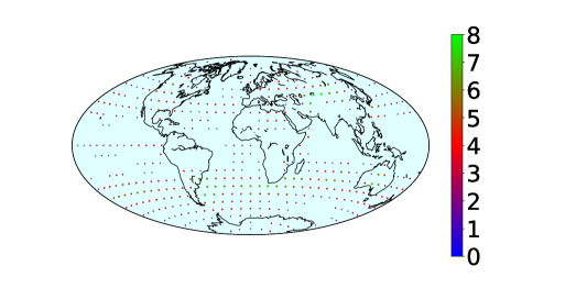
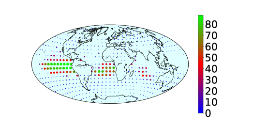
(a)	(b)
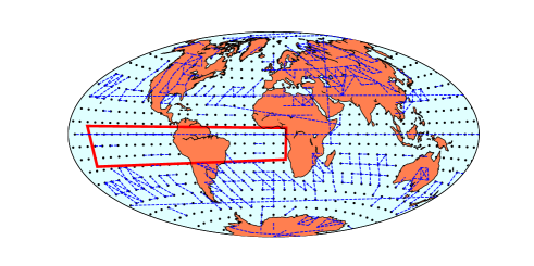
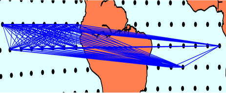
(c)	(d)

Figure 5: (i) The geographic distribution of degrees for the nodes of the network for $C=0.5$ and above (a) One year before a very strong El Niño episode, December 1996. (b) During very strong El Niño episode, December 1997. (ii) The Teleconnection plots of the networks at $C=0.5$ and above (c) One year before a very strong El Niño episode, December 1996. The same quantity in the red rectangular region in (c) is shown during a very strong El Niño episode, December 1997 in (d) indicating the teleconnections between the nodes with degree $\geq 70$.

It can be clearly observed from above plots that during very strong El Niño activity, nodes from the El Niño basin have higher degree ($\geq 40$) and are strongly connected whereas for indicator year nodes have a lower degree distribution range ($0$-$15$) and highly connected nodes appear outside the El Niño basin. We thus have a set of topological signatures for the indicator years of the El Niño episodes in addition to the susceptibility and the microtransitions.

	Year	$C_{c}$	$C_{max}$	$\Delta\chi$	Total
					number
					of links
1.	1981	0.4411	0.7609	22	10108
	04/1982 to 06/1983, (15 months)	0.5419	0.8863	3	24850
2.	1985	0.4536	0.796	30	10601
	09/1986 to 02/1988, (18 months)	0.4879	0.9361	5	20021
3.	1990	0.4682	0.7912	18	10592
	05/1991 to 06/1992, (14 months)	0.4874	0.8513	6	16545
4.	1993	0.4695	0.7787	15	11981
	09/1994 to 03/1995, (7 months)	0.4871	0.8538	4	14099
5.	1996	0.4736	0.843	37	10331
	05/1997 to 05/1998, (13 months)	0.5027	0.952	5	27469
6.	2001	0.466	0.8157	3	10122
	06/2002 to 02/2003, (9 months)	0.4856	0.7986	5	14311
7.	2003	0.4856	0.7984	5	9393
	07/2004 to 02/2005, (8 months)	0.4660	0.7929	7	10000
8.	2005	0.466	0.7929	7	10000
	09/2006 to 01/2007, (5 months)	0.4948	0.8712	2	12830
9.	2008	0.5126	0.8346	6	17882
	07/2009 to 03/2010, (9 months)	0.5119	0.8747	1	24397
10.	2013	0.462	0.7877	27	11170
	11/2014 to 05/2016, (19 months)	0.5022	0.8949	3	20301
11.	2018	0.5001	0.865	4	12919

Table 1: All El Niño events between $1979-2018$ with distinct precursors.

Table [1] summarizes all the distinct and significant indicators for all the El Niño episodes occurring between $1979$ to $2018$. Indicator years are shown in bold font followed by the corresponding El Niño episode or event with its duration. As can be seen, lengths of the episodes vary from a minimum of $5$ months to $19$ months. It is observed that all the indicator years have significantly higher $|\Delta\chi|$ values. We see that when the quantity $|\Delta\chi|$ crosses a threshold value $7$, it can be used as an alarm and it is predicted that an El Niño event will start in the following calendar year. A network is constructed for each year using the data of $\approx 565$ days and a prediction is made at the end of every year ($31^{st}$ December). The lead time between the prediction and the beginning of the El Niño episodes is $\approx 6.42$ months and $\approx 9.57$ months till the time when the episode peaks. It is also observed that magnitude of $|\Delta\chi|$ is distinctly higher for the indicator years followed by strong and very strong El Niño episodes compared to weak or moderate episodes. The value $C_{c}$ at which the network undergoes a discontinuous percolation transition is given in [table 1]. Here, the difference between indicator years and El Niño years can be clearly seen. For indicator years the $C_{c}$ value generally ranges between $0.4411$ to $0.4736$ whereas during the El Niño years $C_{c}$ is shifted towards higher values ($>0.5$). The total number of links for all the values of $C$ in indicator years is about $10,000$, whereas in El Niño years it is between $14,000-20,000$. We observed that when the total number of links crosses the threshold ($8100-9500$), one can expect El Niño in the following calendar year. The number of highly correlated links, with $C$ values $C_{max}$, up to $0.9$ is seen in networks of El Niño years. The node degrees in these years also take high values, as can be seen in Fig.[5(b)]. Some of these quantities can be used as precursors in conjunction with the susceptibility jumps and $C_{c}$ values in years where the El Niño phenomena is mild. Thus, we have identified a comprehensive set of network quantities which can act as clear precursors of El Niño years, in climate networks constructed using surface air temperature data from $1979$ to $2018$. We note that networks constructed for other years do not possess these distinctive features. The El Niño prediction can be made between 4 to 9 months in advance. We also note that our precursors (the jump in the susceptibility $\Delta\chi$ and critical correlation value) miss the prediction of an upcoming moderate El Niño event in the year $2009$-$10$. Nevertheless we observe that out of all the indicators, two indicators i.e. the value of $C_{max}=0.8346$ and the total number of links$=17882$ do suggest an upcoming El Niño event. The node degree plot of the year $2008$ (not shown here), shows nodes of degrees as high as $40$, which also suggests some indication of the $2009$-$10$ El Niño event. Only one false positive alarm is observed in the year $2000$ in the $39$ climate networks studied, where the susceptibility and $C_{c}$ predicted an El Niño in the year $2001$ which did not actually occur. This was due to the presence of a prolonged and strong La Niña episode which lasted $32$ months between July $1998$ to February $2001$. The total number of links and the highest degrees of nodes showed moderate values viz. $11000$ and $16$ in the year $2000$ and were not indicative of an El Niño phenomenon in $2001$. We also observed from the table [1] that year $2018$ has slightly higher values of precursors such as $C_{max}$ ($0.865$), total number of links ($12919$) and nodes of degrees as high as $30$. These values of precursors indicated a weak El Niño episode which was observed in year $2019$. It may be possible to remove these anomalies by using a sliding window for the time averages, or by sampling focused geographic regions. These may also help to identify the tipping points and tipping locations of the phenomena. We also observed stronger link density in the indicator years in the area of polar jet streams, i.e. powerful meandering air currents that arise due to atmospheric heating by solar radiation and the action of the Coriolis force in a generally westerly direction. It appears that jet streams get stronger in the indicator years and show a different pattern for these years depending on the beginning of El Niño (Spring or fall) elena . We hope to quantify and provide further support for this assertion in future work.

To summarize we have identified a set of precursors for the El Niño phenomena, using the construction of climate networks. These include the susceptibility, the value of the critical correlation, the maximum value of the correlation strength and total number of links observed in the climate network. The topological characterizers i.e. the degree distribution and the total number of links, supplement the information available in the order parameter and the susceptibility. These precursors, taken together, constitute signatures of the indicator year which can reliably predict an El Niño event, four to ten months in advance, and significantly reduce the frequency of false alarms. We hope our methods provide pointers for other investigations in the context of climate networks.

I Acknowledgement

RS thanks IIT Madras for an Institute postdoctoral fellowship for the period in which this work was done.

References

- (1) J. Deza, M. Barreiro, and C. Masoller, Eur. Phys. J.: Spec. Top. 222, 511 (2013).
- (2) M. Barreiro, A. C. Marti, and C. Masoller, Chaos 21, 013101 (2011).
- (3) A. A. Tsonis, K. L. Swanson, and P. J. Roebber, Bull. Am. Meteorol. Soc. 87, 585 (2006).
- (4) N. Malik, B. Bookhagen, N. Marwan, and J. Kurths, Clim. Dyn. 39, 971 (2012).
- (5) V. Stolbova, E. Surovyatkina, B. Bookhagen, J. Kurths, Geophys. Res. Lett. 43, 3982 (2016).
- (6) K. Yamasaki, A. Gozolchiani and S. Havlin, Phys. Rev.Lett. 100, 228501 (2008).
- (7) A. A. Tsonis and K. L. Swanson, Phys. Rev. Lett. 100, 228502 (2008).
- (8) J. F. Donges, Y. Zou, N. Marvan and J. Kurths, Eur. Phys. J. Spec. Top. 174, 157 (2009).
- (9) J. F. Donges, Y. Zou, N. Marvan and J. Kurths, Europhys. Lett. 87, 48007 (2009).
- (10) A. Gozolchiani, S. Havlin and K. Yamasaki, Phys. Rev. Lett. 107, 148501 (2011).
- (11) Y. Wang, A. Gozolchiani, Y. Ashkenazy, Y. Berezin, O. Guez and S. Havlin, Phys. Rev. Lett. 111, 138501 (2013).
- (12) D. Zhou, A. Gozolchiani, Y. Ashkenazy and S. Havlin, Phys. Rev. Lett. 115, 268501 (2015).
- (13) M. S. Halpert and C. F. Ropelewski, J. Clim. 5, 577 (1992).
- (14) Late Victorian Holocausts: El Niño Famines and the Making of the Third World, M. Davis, Verso, London (2001).
- (15) The European Centre for Medium-Range Weather Forecasts (ECMWF) is an independent intergovernmental organisation,(http://apps.ecmwf.int/datasets/data/interim-full-daily/levtype=pl/)
- (16) V. Rodríguez-Méndez, V. Eguíluz, E. Hernández-García and J. Ramasco, Sci. Rep. 6, 29552 (2016).
- (17) M. Scheffer, J. Bascompte, W. Brock, V. Brovkin, S. Carpenter, V. Dakos, H. Held, E. van Nes, M. Rietkerk and G. Sugihara, Nature 461, 08227 (2009).
- (18) D. Stauffer and A. Aharony, Introduction to Percolation Theory, Taylor & Francis, London, (1994).
- (19) W. Chen, M. Schröder, R. M. D’Souza, D. Sornette and J. Nagler, Phys. Rev. Lett. 112, 155701 (2014).
- (20) J. Meng, J. Fan, Y. Ashkenazy, and S. Havlin, CHAOS 27, 035807 (2017).
- (21) O. Guez, A. Gozolchiani and S. Havlin, Phys. Rev. E 90 062814 (2014).
- (22) Prof. E. Surovyatkina, Private communication.