The Sixth Data Release of the Radial Velocity Experiment (Rave) – II: Stellar Atmospheric Parameters, Chemical Abundances and Distances

Abstract

We present part 2 of the 6th and final Data Release (DR6 or FDR) of the Radial Velocity Experiment (Rave), a magnitude-limited ($9<I<12$) spectroscopic survey of Galactic stars randomly selected in the southern hemisphere. The Rave medium-resolution spectra ($R\sim 7500$) cover the Ca-triplet region ($8410-8795$ Å) and span the complete time frame from the start of Rave  observations on 12 April 2003 to their completion on 4 April 2013. In the second of two publications, we present the data products derived from 518 387 observations of 451 783 unique stars using a suite of advanced reduction pipelines focussing on stellar atmospheric parameters, in particular purely spectroscopically derived stellar atmospheric parameters ($T_{\mathrm{eff}}$, $\log g$, and the overall metallicity), enhanced stellar atmospheric parameters inferred via a Bayesian pipeline using Gaia DR2 astrometric priors, and asteroseismically calibrated stellar atmospheric parameters for giant stars based on asteroseismic observations for 699 K2 stars. In addition, we provide abundances of the elements Fe, Al, and Ni, as well as an overall $[\mathrm{\alpha}/\mathrm{Fe}]$ ratio obtained using a new pipeline based on the GAUGUIN optimization method that is able to deal with variable signal-to-noise ratios. The Rave DR6 catalogs are cross matched with relevant astrometric and photometric catalogs, and are complemented by orbital parameters and effective temperatures based on the infrared flux method. The data can be accessed via the Rave  Web site or the Vizier database.

1 Introduction

Wide-field spectroscopic surveys of the stellar content of the Galaxy provide crucial information on the combined chemical and dynamical history of the Milky Way, and for the understanding of the formation and evolution of galaxies in a broader context. Spectroscopy enables us to measure the radial velocities of stars, which, when combined with positions, distances and proper motions from astrometry, allows us to study Galactic dynamics in detail. Spectroscopy also enables us to measure atmospheric properties (surface gravity $\log g$ and effective temperature $T_{\mathrm{eff}}$) of stars and the abundance of chemical elements in the stellar atmosphere, thus providing important clues on the chemical evolution of the Galaxy and of its stellar populations (see, e.g., Freeman & Bland-Hawthorn, 2002, who also coined the term Galactic Archaeology for this type of research). The combination of large wide-field spectroscopic surveys with massive and precise astrometric information as delivered by the Gaia mission (Gaia Collaboration et al., 2016a) is particular powerful, as demonstrated by a large number of publications in the past two years.

The scientific potential of combining wide-field spectroscopy and astrometry has been motivation for a number of spectroscopic Galactic Archaeology surveys, starting with the Geneva-Copenhagen survey (CGS, Nordström et al., 2004) and the Radial Velocity Experiment (Rave, Steinmetz, 2003), followed by a meanwhile considerable number of surveys of similar or even larger size at lower (e.g., SEGUE, Yanny et al. 2009; and LAMOST, Zhao et al. 2012) and higher spectral resolution (e.g., APOGEE, Majewski et al. 2017; GALAH, De Silva et al. 2015; and Gaia-ESO, Gilmore et al. 2012). For a recent review on abundances derived from large spectroscopic surveys we refer to Jofré et al. (2019).

This publication addresses the determination of stellar atmospheric parameters, chemical abundances, and distances in the context of the Rave survey, which over its 10 year observing campaign amassed this information based on more than half a million spectra. Together with the accompanying paper (Steinmetz et al., 2020, henceforth DR6-1), which is focusing on Rave  spectra, error spectra, spectral classification, and radial velocity determinations, it constitutes the sixth and final data release (DR6) of Rave. In particular, DR6 provides a new set of stellar atmospheric parameters employing parallax information from Gaia DR2 (Gaia Collaboration et al., 2018), and a robust determination of the $\alpha$-enhancement $[\mathrm{\alpha}/\mathrm{Fe}]$.

The paper is structured as follows: in Section 2 we give a brief overview of the Rave survey and its collected data. Section 3 presents an update on the stellar atmospheric parameter determination and introduces a new catalog of stellar stellar atmospheric parameters inferred using a Bayesian pipeline with Gaia DR2 parallax priors following the procedure outlined in McMillan et al. (2018). In Section 4, a new optimization pipeline GAUGUIN is presented (Bijaoui et al., 2010, 2012; Guiglion et al., 2016) in order to extract $[\mathrm{\alpha}/\mathrm{Fe}]$ ratios as well as individual abundances of Fe, Al, and Ni. Section 5 describes how orbital parameters of stars are derived from Rave combined with Gaia DR2 astrometric information. Rave data validation including a comparison of Rave  stellar stellar atmospheric parameters and abundances with external observational data sets is done in Section 6. Section 7 presents the Rave  DR6 catalog, followed by a reanalysis of some previously published Rave  results in order to demonstrate the capabilities of Rave  DR6 (Section 8). Finally, Section 9 gives a summary and draws some conclusions.

2 Survey Data and their reduction

The motivation, history, specifications and performance of the Rave survey are presented in detail in the data release papers DR1, DR2, DR3, DR4, and DR5 (Steinmetz et al., 2006; Zwitter et al., 2008; Siebert et al., 2011a; Kordopatis et al., 2013a; Kunder et al., 2017) and a comprehensive summary is given in DR6-1 (Steinmetz et al., 2020). Here, we only summarize the main properties of the Rave survey.

Rave was initiated in 2002 as a kinematically unbiased wide-area survey of the southern hemisphere with the primary goal to determine radial velocities of Milky Way stars (Steinmetz, 2003). Thanks to the 6dF multi-object spectrograph on the 1.23m UK Schmidt telescope at Siding Spring in Australia, up to 150 spectra could be simultaneously acquired over a field of view of 5.7°. Spectra were taken at an average resolution of $R=7500$ over the IR Ca triplet region at $8410-8795$ Å, which is similar in coverage and somewhat lower in resolution when compared to the spectral range probed by the Gaia RVS instrument ($R_{\text{RVS}}=11500$, Cropper et al., 2018).

The targets of RAVE are mainly drawn from a magnitude range $9<I<12$, where $I$ is Cousins $I$. At an exposure time of typically 1 hour, a signal-to-noise (SNR) of $\hbox{SNR}\approx 40$ can be achieved for targets between $I\approx 10-11$ (see DR6-1 for details). Since a 6dF fibre corresponds to $6.7\arcsec$ on the sky, Rave observing avoided the bulge region and disk regions at low Galactic latitude in order to minimize contamination by unresolved multiple sources within a single fiber.

The input catalog of Rave was initially produced by a combination of the Tycho-2 catalog (Høg et al., 2000) and the Supercosmos Sky Survey (SSS, Hambly et al., 2001). Later on, upon availability, the input catalogue was converted to the DENIS (Epchtein et al., 1997) and 2MASS (Skrutskie et al., 2006) system.

Since Rave was designed as a survey with its main focus on studies of Galactic dynamics and Galactic evolution, the observing focus was to approach an unbiased target selection with a wide coverage of the accessible sky. Consequently most targets were only observed once. In order to account, at least statistically, for the effects of binarity, about 4000 stars were selected for a series of repeat observations roughly following a logarithmic series with a cadence of separations of 1, 4, 10, 40, 100, and 1000 days (see DR6-1, Section 2.7 for details).

During the overall observing campaign of Rave, which lasted from 12 April 2003 to 4 April 2013, 518,387 spectra for 451,783 stars where successfully taken and reduced.

The data reduction of Rave  follows the sequence of the following pipeline:

1. quality control of the acquired data on site with the RAVEdr software package (paper DR6-1, Section 3.1).

2. reduction of the spectra (DR6-1, Section 3.1).

3. spectral classification (DR6-1, Section 4).

4. determination of (heliocentric) radial velocities with SPARV (‘Spectral Parameter And Radial Velocity’, DR6-1, Section 5).

5. determination of stellar atmospheric parameters $T_{\mathrm{eff}}$  $\log g$, and $[{\rm m}/{\rm H}]$ with MADERA (‘MAtisse and DEgas used in RAve’, (Section 3.1).

6. determination of the effective temperature using additional photometric information (InfraRed Flux Method (IRFM), Section 3.2).

7. modification of the Rave  stellar atmospheric parameters $T_{\mathrm{eff}}$  $\log g$, and $[{\rm M}/{\rm H}]$ derived spectroscopically with additional photometry and Gaia DR2 parallax priors using BDASP (Bayesian Distances Ages and Stellar Parameters, DR6-2 Section 3.3).

8. determination of the abundance of the elements Fe, Al, and Ni, and an overall $[\mathrm{\alpha}/\mathrm{Fe}]$ ratio with the pipeline GAUGUIN (Section 4).

9. recalibration of the stellar atmospheric parameters $T_{\mathrm{eff}}$  $\log g$, and $[{\rm M}/{\rm H}]$, for giant stars based on K2 asteroseismic information (Section 3.4) followed by the determination of the chemical abundances $[\mathrm{Fe}/\mathrm{H}]$ and $[\mathrm{Mg}/\mathrm{H}]$ using the GAUFRE pipeline (Valentini et al., 2013).

The output of these pipelines is accumulated in a PostgreSQL data base and accessible via the Rave  website http://www.rave-survey.org (Section 7 and DR6-1, Section 7).

3 Stellar Atmospheric Parameters

3.1 Stellar Atmospheric Parameters from Spectroscopy

Rave DR6 employs the exact same procedure to derive stellar atmospheric parameters from spectroscopy as DR5 (Kunder et al., 2017). In short, the pipeline MADERA uses a combination of (i) a decision tree (DEGAS, Bijaoui et al., 2012), which normalizes the spectrum iteratively as well as parameterizing the low SNR spectra, and (ii) a projection algorithm (MATISSE, Recio-Blanco et al., 2006) which is used to obtain the stellar atmospheric parameters for the high SNR spectra ($>30$).

Both of the methods are used with the grid of 3580 synthetic spectra first calculated in the framework of Kordopatis et al. (2011) and adjusted for DR4 (Kordopatis et al., 2013a) assuming the Solar abundances of Grevesse (2008) and Asplund et al. (2005). This grid has been computed using the MARCS model atmospheres (Gustafsson et al., 2008) and Turbospectrum (Plez, 2012) under the assumption of local thermodynamic equilibrium (LTE). The atomic data was taken from the VALD database (Kupka et al., 2000), with updated oscillator strenghts from Gustafsson et al. (2008). The line-list has been calibrated primarily on the Solar spectrum of Hinkle et al. (2003) and with adjustments to fit also the Arcturus spectrum to an acceptable level (see Kordopatis et al., 2011, for further information). Furthermore, the grid excludes the cores of the Calcium triplet lines, as they can suffer, depending on spectral type, from non-LTE effects or emission lines owing to stellar activity. The grid has three free parameters: effective temperature, $T_{\mathrm{eff}}$, logarithm of the surface gravity, $\log g$, and metallicity, $[{\rm m}/{\rm H}]$. These free parameters are hence the parameters that MADERA determines.

We note that the $\alpha$ enhancement $[\mathrm{\alpha}/\mathrm{Fe}]$ varies across the grid, but is not a free parameter. Indeed, only one $[\mathrm{\alpha}/\mathrm{Fe}]$ value is adopted per $[{\rm m}/{\rm H}]$ grid-point:

$$\left[\frac{\alpha}{\mathrm{Fe}}\right]=\left\{\begin{array}[]{rl}+0.4\quad:&\left[\frac{\mathrm{m}}{\mathrm{H}}\right]\leq-1\\ &\\ -0.4\times\left[\frac{\mathrm{m}}{\mathrm{H}}\right]\quad:&-1<\left[\frac{\mathrm{m}}{\mathrm{H}}\right]<0\\ &\\ 0\quad:&\left[\frac{\mathrm{m}}{\mathrm{H}}\right]\geq 0\end{array}\right.$$ (1)

This implies that the $[{\rm m}/{\rm H}]$ value of the grid can be thought of as the content of all the metals in the star, except the $\alpha$ elements. The derived value of $[{\rm m}/{\rm H}]$  from an observed spectrum, denoted by $\hbox{$[{\rm m}/{\rm H}]$}_{u}$, should hence be considered as an overall metallicity estimator assuming an $\alpha$-enhancement. This should be discriminated from methods and grids based on the total metallicity including an $\alpha$ enhancement, like those used in Section 3.3 and 3.4, we refer to those metallicity estimators as $[{\rm M}/{\rm H}]$.

Finally, with $[\mathrm{Fe}/\mathrm{H}]$ we refer to direct measurements of the iron content by fitting iron line,

e.g. with the GAUGUIN method (Section 4) or when using high resolution data for validation (see Section 6).

3.1.1 MADERA’s quality flags

In addition to the stellar atmospheric parameters ($T_{\mathrm{eff}}$, $\log g$, $[{\rm m}/{\rm H}]$) and their associated uncertainties, the pipeline provides each spectrum with one of the five quality flags (algo_conv_madera) given below to allow the user to filter, quite robustly, the results according to adopted criteria that are sound and objective (e.g., convergence of the algorithm):

• ‘0’: The analysis was carried out as desired. The normalization process converged, as did MATISSE (for high SNR spectra) or DEGAS (for low SNR spectra). There are 322,367 spectra that fulfill this criterion.

• ‘1’: Although the spectrum has a sufficiently high SNR to use the projection algorithm, the MATISSE algorithm did not converge. Stellar atmospheric parameters for stars with this flag are not reliable. There are 17,639 spectra affected by this.

• ‘2’: The spectrum has a sufficiently high SNR to use the projection algorithm, but MATISSE oscillates between two solutions. The reported parameters are the mean of these two solutions. In general, the oscillation happens for a set of parameters that are nearby in parameter space and computing the mean is a sensible thing to do. However, this is not always the case, for example, if the spectrum contains artifacts. The mean may then not provide accurate stellar atmospheric parameters. The 58,992 spectra with a flag of ‘2’ could be used for analyses, but with caution (a visual inspection of the observed spectrum and its solution may be required).

• ‘3’: MATISSE gives a solution that is extrapolated to values outside of the parameter range defining the learning grid ($T_{\rm eff}$ outside the range [3500,8000] K, $\log g$ outside of the range [0,5.5], metallicity outside the range [-5,+1] dex), and the solution is forced to be the one from DEGAS. For spectra having artifacts but high SNR overall, this is a sensible thing to do, as DEGAS is less sensitive to such discrepancies. This applies to 87,335 spectra. However, for the few hot stars that have been observed by Rave, adopting this approach is not correct. A flag of ‘3’ and a $T_{\rm eff}>$ 7750 K is very likely to indicate that this is a hot star with $T_{\rm eff}>$ 8000 K and hence that the parameters associated with that spectrum are not reliable.

• ‘4’: This flag will only appear for low SNR stars and metal-poor giants. Indeed, for metal-poor giants, the spectral lines available are neither strong enough nor numerous enough to have DEGAS successfully parameterize the star. Tests on synthetic spectra have shown that to derive reliable parameters the settings used to explore the branches of the decision tree need to be changed compared to the ‘standard’ parameters adopted for the rest of the parameter space. A flag ‘4’ therefore marks this change in the setting for book-keeping purposes, and the 31,488 spectra associated with this flag should be safe for any analysis.

3.1.2 Calibration of the stellar atmospheric parameters

Several tests performed for DR4 as well as the subsequent science papers, have indicated that the stellar parameter pipeline is globally robust and reliable. However, being based on synthetic spectra that may not match the real stellar spectra over the entire parameter range, the direct outputs of the pipeline need to be calibrated on reference stars in order to minimize possible systematic offsets.

To calibrate the DR6 outputs of the pipeline, the same calibration data-set and polynomial fit compared to literature values has been used as for DR5. For completeness reasons, we review the relations in the following subsections, but refer the reader to the DR4 and DR5 papers for further details. We performed tests with additional subsets (coming from e.g. asteroseismic surface gravities) or/and more complex polynomials to calibrate the pipeline’s output and obtained results that did not show any significant improvement over the approach that was adopted in DR4 and DR5.

Metallicity calibration

The calibration relation for DR6 is:

$$\begin{split}\hbox{$[{\rm m}/{\rm H}]$}_{\rm DR6}=\hbox{$[{\rm m}/{\rm H}]$}_{\rm u}+(0.276-0.044~{}{\hbox{$\log g$}_{\rm u}}\\ +0.002~{}{\hbox{$\log g$}_{\rm u}^{2}}-0.248~{}\hbox{$[{\rm m}/{\rm H}]$}_{\rm u}\\ +0.007~{}{\hbox{$[{\rm m}/{\rm H}]$}_{\rm u}}~{}{\hbox{$\log g$}_{\rm u}}-0.078~{}{\hbox{$[{\rm m}/{\rm H}]$}_{\rm u}^{2})},\vskip 12.0pt plus 4.0pt minus 4.0pt\end{split}$$ (2)

where $\hbox{$[{\rm m}/{\rm H}]$}_{\rm DR6}$ is the calibrated metallicity, and $\hbox{$[{\rm m}/{\rm H}]$}_{\rm u}$ and $\hbox{$\log g$}_{\rm u}$ are, respectively, the un-calibrated metallicity and surface gravity (both the raw output from the pipeline). The adopted calibration corrects for a rather constant underestimation of 0.2 dex at the lowest metallicities, while also correcting trends in the more metal-rich regimes, where the giant stars exhibit higher offets than the dwarfs. As already described in the earlier DR papers, this relation has been calibrated against $[\mathrm{Fe}/\mathrm{H}]$ values from the literature. This implies that $\hbox{$[{\rm m}/{\rm H}]$}_{\rm DR6}$ is a proxy for $[\mathrm{Fe}/\mathrm{H}]$ only if all of the elements in the targeted star are solar-scaled and if the $\alpha$ abundances are following the same relation as adopted for the synthetic grid at the $[\mathrm{Fe}/\mathrm{H}]$ value of the star of interest. $\hbox{$[{\rm m}/{\rm H}]$}_{\rm DR6}$ should therefore be rather thought of as a metallicity indicator, i.e. to depend on a combination of elements. $\hbox{$[{\rm m}/{\rm H}]$}_{\rm DR6}$ is, however, not equal to the overall metallicity of the star, as discussed above - see also equation 5 in section 3.3).

Surface gravity calibration

The following quadratic expression defines our surface gravity calibration:

$$\hbox{$\log g$}_{\rm DR6}=\hbox{$\log g$}_{\rm u}+(0.515-0.026~{}{\hbox{$\log g$}_{\rm u}}-0.023~{}{\hbox{$\log g$}_{\rm u}^{2}}).$$ (3)

This relation increases gravities of supergiants by $\sim 0.5$ dex, and of dwarfs by $\sim 0.75$ dex.

Effective temperature calibration

The adopted calibration for effective temperature is

$$\rm T_{\rm eff,DR6}=T_{\rm eff,u}+(285\,\text{K}-0.073{T_{\rm eff,u}}+40\,\text{K}\times{\hbox{$\log g$}_{\rm u}}).$$ (4)

Corrections reach up to 200 K for cool dwarfs, but are generally much smaller.

3.2 Infrared Flux Method Temperatures

Effective temperatures from the infrared flux method (IRFM, Casagrande et al., 2006, 2010) are derived in a manner similar to that carried out in Rave  DR5, where a detailed description can be found. Briefly, our implementation of the IRFM uses APASS and 2MASS photometry to recover stellar bolometric and infrared fluxes. The ratio of these two fluxes for a given star is compared to that predicted from theoretical models, for a given set of stellar atmospheric parameters, and an iterative approach is used to converge on the final value of $T_{\mathrm{eff}}$. The advantage of comparing observed versus model fluxes in the infrared is that this region is largely dominated by the continuum and thus very sensitive to $T_{\mathrm{eff}}$, while the dependence on surface gravity and metallicity is minimal. Here, we adopt for each star the calibrated $\hbox{$\log g$}_{\rm DR6}$ and $\hbox{$[{\rm m}/{\rm H}]$}_{\rm DR6}$ from the MADERA pipeline, but if we were instead to use the parameter values from the SPARV pipeline the derived value of $T_{\mathrm{eff}}$ would differ by a few tens of Kelvin at most. Since the IRFM simultaneously determines bolometric fluxes and effective temperatures, stellar angular diameters can be derived, and are also provided in DR6. Extensive comparison with interferometric angular diameters to validate this method is discussed in Casagrande et al. (2014). We are able to provide $T_{\mathrm{eff}}$ from the IRFM for over 90% of our sample, while for about 6% of them we have to resort to color-temperature relations derived from the IRFM. For less than 3% of our targets effective temperatures could not be determined due to the lack of reliable photometry.

In a photometric method such as the IRFM, reddening can have a non-negligible impact. We rescale the reddening from Schlegel et al. (1998) as described in Rave DR5, but for stars with $\log(g)<3.5$ and $E(B-V)>0.3$ we now use the relation $E(B-V)=0.918(H-W2-0.08)/0.366$ from the Rayleigh–Jeans color excess method (RJCE, Majewski et al., 2011).

3.3 Distances, Ages, Stellar Atmospheric Parameters with Gaia priors

Rave DR6 includes for the first time stellar atmospheric parameters derived using the Bayesian framework demonstrated in McMillan et al. (2018), along with derived distances, ages, and masses, which have also been derived for previous data releases. We refer to the method as the BDASP code. This follows the pioneering work deriving (primarily) distances by Burnett & Binney (2010) and Binney et al. (2014).

This method takes as its input the stellar atmospheric parameters $T_{\mathrm{eff}}$ (taken from the IRFM, Section 3.2), $\log g$ taken from the MADERA pipeline, an estimate of the overall metallicity taken from the MADERA (see below), $J$, $H$, and $K_{s}$ magnitudes from 2MASS, and, for the first time, parallaxes from Gaia DR2. For a detailed description of the method, the interested reader should refer to McMillan et al. (2018), where parallaxes from Gaia DR1 (Gaia Collaboration et al., 2016b) were used for the 219,566 Rave  sources which entered the TGAS part of the Gaia catalog (Michalik et al., 2015). Here we simply give a brief overview and note differences in the methodology used here and by McMillan et al. (2018).

BDASP applies the simple Bayesian statement

$$P(\hbox{model}|\hbox{data})=\frac{P(\hbox{data}|\hbox{model})P(\hbox{model})}{P(\hbox{data})},$$

where in our case “data” refers to the inputs described above for a single stars, and “model” comprises a star of specified initial mass ${\cal M}$, age $\tau$, metallicity $[{\rm M}/{\rm H}]$, and location, observed through a specified line-of-sight extinction. $P(\hbox{data}|\hbox{model})$ is determined assuming uncorrelated Gaussian uncertainties on all inputs, and using PARSEC isochrones (Bressan et al., 2012) to find the values of the stellar atmospheric parameters and absolute magnitudes of the model star. The uncertainties of the stellar atmospheric parameters are assumed to be the quadratic sum of the quoted internal uncertainties and the external uncertainties, as found for Rave  DR5 (Kunder et al., 2017, Table 4). $P(\hbox{model})$ is our prior, and $P(\hbox{data})$ is a normalization that we can safely ignore. We adopt the ‘Density’ prior from McMillan et al. (2018), which is the least informative prior considered in that study. Even with the, significantly less precise, Gaia DR1 parallax estimates, the choice of prior had a limited impact on the results, and this is reduced still further because of the very high precision of the Gaia DR2 parallax estimates.

As discussed above, the MADERA pipeline provides $[{\rm m}/{\rm H}]$, the metal content except the alpha elements, which is calibrated against $[\mathrm{Fe}/\mathrm{H}]$. To provide an estimate of the overall metallicity $[{\rm M}/{\rm H}]$ we assume that we can scale all abundances with $[{\rm m}/{\rm H}]$ except those of $\alpha$-elements, which we assume all scale in the same way assumed by MADERA (i.e. following equation 1). A proxy for the overall metallicity including $\alpha$ elements, denoted by $[{\rm M}/{\rm H}]$, can then be inferred by applying a modified version of the Salaris et al. (1993) formula, derived using the same technique as in Valentini et al. (2018):

$$\left[\frac{\mathrm{M}}{\mathrm{H}}\right]=\left[\frac{\mathrm{m}}{\mathrm{H}}\right]_{\rm DR6}+\log_{10}(C\times 10^{\hbox{$[\mathrm{\alpha}/\mathrm{Fe}]$}}+(1-C)),$$ (5)

with $C=0.661$. Within this approximation [M/H] corresponds to the composition assumed by the PARSEC isochrones.

As was made clear at the time of Gaia DR2, astrometric measurements from Gaia have small but significant systematic errors (including an offset of the parallax zero-point), which vary across the sky on a range of scales, and are dependent on magnitude and color (Lindegren et al., 2018; Arenou et al., 2018). This has been demonstrated for a variety of comparison samples since Gaia DR2 (Sahlholdt & Silva Aguirre, 2018; Graczyk et al., 2019; Stassun & Torres, 2018; Zinn et al., 2018; Khan et al., 2019). The parallaxes used in BDASP are therefore corrected for a parallax zero-point of $-54\,\mu{\rm as}$, following the analysis of Schönrich, McMillan, & Eyer (2019). This study determined this zero-point offset for stars with Gaia DR2 radial velocities, which cover a similar magnitude range to Rave, and have a larger zero-point offset than the fainter quasars considered by Lindegren et al. (2018). We also add a systematic uncertainty of $43\,\mu{\rm as}$ in quadrature with the quoted parallax uncertainties to reflect a best estimate of the small-scale spatially varying parallax offsets as found by Lindegren et al. (2018).

In DR5 we provided an improved description of the distances to stars with a multi-Gaussian fit to the probability density function (pdf) in distance modulus. This was particularly important for stars with multi-modal pdfs, for example stars where there was an ambiguity over whether they were subgiants or dwarfs. With the addition of Gaia parallaxes, these ambiguities have become rare. Fewer than one percent of the sources required multi-Gaussian pdfs under the selection criteria used in McMillan et al. (2018). These are generally pdfs with a narrow peak associated with the red clump and an overlapping broader one associated stars ascending the red giant branch, rather than truly multi-modal pdfs (see Binney et al., 2014, for discussion and examples). In the interests of simplicity, we therefore do not provide these multi-Gaussian pdfs with DR6. Extinction is taken into account in the same way as in Binney et al. (2014) and McMillan et al. (2018), and is relatively weak for the majority of RAVE stars. The median extinction we find corresponds to $A_{V}\sim 0.2\,{\rm mag}$, which is $\sim 0.06\,{\rm mag}$ in the $J$-band (the band that suffers the most extinction of all those we consider).

We can use the Gaia DR2 parallaxes to validate our Bayesian distance finding method in the same way as McMillan et al. (2018) did with the TGAS parallaxes: comparing the parallax estimates using BDASP without including the Gaia parallax, to the Gaia DR2 parallax. Since these are independent estimates, we would expect that if we take the difference between these values divided by their combined uncertainty (the two uncertainties summed in quadrature), it will be distributed as a Gaussian, with average zero and standard deviation unity.

In Figure 1 we plot histograms showing this comparison for the parallax estimates from Rave  DR5 (using the same techniques described here, and using MADERA $T_{\mathrm{eff}}$), or using BDASP but taking the IRFM $T_{\mathrm{eff}}$ as input (as this was shown to be a better approach by McMillan et al., 2018). In both cases we show the comparison to the quoted values from Gaia DR2, and a comparison to the ‘adjusted’ values, where we have corrected the Gaia parallaxes for their assumed zero-point offset and systematic uncertainties. This figure demonstrates that the parallax zero-point offset of Gaia is significant, even for these relatively nearby stars. Including the zero-point offset brings the Gaia parallaxes more in line with those from Rave. We also see that the use of IRFM temperatures significantly improves the BDASP parallaxes. In all cases we see more outlying values than we would expect for a Gaussian distribution. One could, therefore, reasonably argue that we should be using the median, rather than a sigma-clipped mean (as in Figure 1) to quantify the bias of the values. The median values, compared to the zero-point adjusted Gaia parallaxes, are 0.136 and 0.011 using MADERA $T_{\mathrm{eff}}$ or IRFM $T_{\mathrm{eff}}$, respectively.

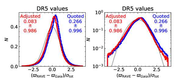
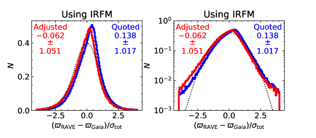
Figure 1: Comparison of Gaia DR2 parallaxes and the purely spectro-photometric parallaxes derived by BDASP for Rave  DR5 using MADERA $T_{\mathrm{eff}}$ (top) and using IRFM $T_{\mathrm{eff}}$ (bottom). The colors indicate whether we are using the parallaxes as quoted by Gaia DR2 (blue), or adjusted for a parallax zero-point of $-54\,\mu{\rm as}$, and systematic uncertainty of $43\,\mu{\rm as}$ (red). The black dotted line is a normal distribution of mean zero and standard deviation unity. The right-hand panels show the same data as the left-hand ones, but with a logarithmic y-axis to emphasize the tails of the distribution. The numbers given in the top corners of each panel are the mean and standard deviation of the values (considering only values between $-4$ and $4$).

We can compare the precision we achieve for stellar atmospheric parameters with BDASP in Rave DR6 to the precision achieved with MADERA. The most interesting of these is the precision in $\log g$, where the Gaia parallax provides the greatest value. This comparison is shown in Figure 2, and we see that we improve by more than a factor of two (median precision $0.16\,$dex for MADERA, $0.07$ dex for BDASP). The dwarf stars, which are nearby and therefore have precise parallax estimates from Gaia, dominate the narrow peak at the smaller BDASP $\log g$ uncertainties of $\sim 0.04\,{\rm dex}$ while giants make up most of the broader peak of larger $\log g$ uncertainties. We can also compare the distance uncertainty BDASP found without Gaia DR2 parallax input in Rave DR5, as compared to the distance uncertainty now. Here we find a dramatic improvement, from a typical distance uncertainty of 30 percent in DR5 to one of 4 percent in DR6. Furthermore, Gaia DR2 parallaxes are available for 99.8% of Rave spectra, as opposed to only 49% in Rave DR5/Gaia DR1. At this point the only significant gain in precision of using spectro-photometric information to derive distances for RAVE stars is for the red clump and high on the giant branch (the latter being known to be problematic for RAVE: McMillan et al., 2018). Otherwise the distance estimates are, to a fairly close approximation, derived directly from Gaia parallaxes, so it makes little difference whether these distances, or the ones derived directly from Gaia parallaxes alone are used. This reflects the extraordinary precision of Gaia DR2, and emphasizes the value of combining the Gaia data with Rave.

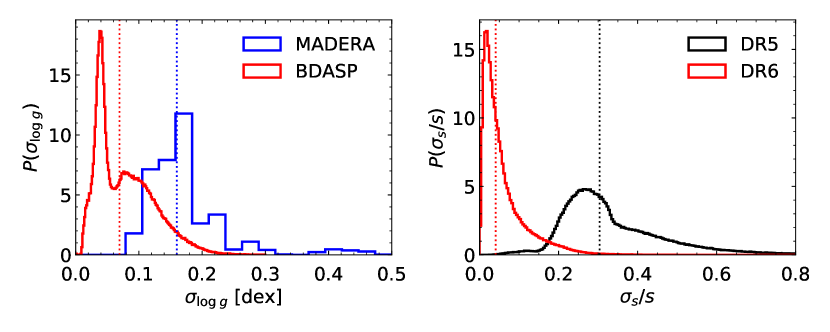
Figure 2: Histograms of quoted uncertainties, demonstrating the improved precision when including information from Gaia DR2 parallax values in the BDASP framework. Left: Comparison of the quoted $\log g$ uncertainty from MADERA alone (blue) as compared to those from BDASP (which has MADERA $\log g$ as one of its inputs: red). Right: Comparison of the relative uncertainties in distance found by BDASP in Rave DR5 (which did not have Gaia parallaxes as input: black) and DR6 (which does: red).

3.4 Asteroseismically calibrated red giant catalog

The surface gravity provided by asteroseismology ($\hbox{$\log g$}_{\rm S}$) is now widely used for testing the accuracy of the $\log g$ measured from spectroscopy. The seismic $\hbox{$\log g$}_{\rm S}$ can be easily computed starting from the scaling relations, two relations that directly connect stellar mass and radius to the effective temperature ($T_{\mathrm{eff}}$) and two seismic observables $\Delta\nu$ (average frequency separation) and $\nu_{\mathrm{max}}$(frequency of maximum oscillation power). The seismic $\hbox{$\log g$}_{\rm S}$ depends only on $T_{\mathrm{eff}}$ and $\nu_{\mathrm{max}}$, and it is defined as:

$$\hbox{$\log g$}_{\rm S}=\hbox{$\log g$}_{\odot}+\log\left(\frac{\hbox{$\nu_{\mathrm{max}}$}}{\hbox{$\nu_{\mathrm{max}}$}_{\odot}}\right)+\frac{1}{2}\log\left(\frac{\hbox{$T_{\mathrm{eff}}$}}{\hbox{$T_{\mathrm{eff}}$}_{\odot}}\right)$$ (6)

where the solar values are $\hbox{$\log g$}_{\odot}$=4.44 dex, $\hbox{$\nu_{\mathrm{max}}$}_{\odot}$= 3090$\,\mu$Hz, and $\hbox{$T_{\mathrm{eff}}$}_{\odot}=5777$ K (Huber et al., 2011).

Large spectroscopic surveys as APOGEE, Gaia-ESO, LAMOST, and GALAH observed seismic targets with the purpose of testing and calibrating, if necessary, the $\log g$ measured by their spectroscopic pipelines. Thanks to the recommissioned Kepler satellite, the K2 mission (Howell et al., 2014), Rave  had the opportunity to incorporate seismic data starting in DR5 (Kunder et al., 2017), where a set of 87 red giant stars, observed by K2 in Campaign 1, were used as calibrators and for an ad hoc calibration for red giant stars only (Valentini et al., 2017). In DR6, 699 red giants observed during the first six K2 campaigns are used (see Table 1, showing the number of targets per campaign). This allowed for an improved coverage of the parameter space (in particular, effective temperature and metallicity). We use the procedure as outlined in DR5, but use $\hbox{$T_{\mathrm{eff}}$}_{\mathrm{,IRFM}}$ as the prior for the effective temperature. We also allow a larger flexibility interval ($\pm 450\,$ K instead of 350 K as in Valentini et al. (2017). The calibration adopted in this case turned out to be very similar to the one in DR5, confirming the robustness of the method, given the larger seismic data set. For the catalog presented in the later part of this work (Section 7.3):

$${\hbox{$\log g$}_{\mathrm{S}}}=\hbox{$\log g$}_{u}-0.76^{0.80}_{0.74}\times\hbox{$\log g$}_{u}+1.98^{2.06}_{1.90}\qquad,$$ (7)

where $\hbox{$\log g$}_{u}$ is the un-calibrated $\log g$ delivered by the MADERA pipeline. Further details on the seismic and spectroscopic data analysis are presented in Valentini et al. (2020, in prep).

Asteroseismology can be also used for providing estimates of the mass of red giants, and hence their age (since the age of a red giant corresponds to the time it spent on the main sequence, and therefore its mass). In Valentini et al. (2020, in preparation) we derive mass, radius, and distance of the K2-Rave  stars using PARAM (Rodrigues et al., 2017), a Bayesian tool that infers stellar properties using both atmospheric and seismic parameters as input.

Table 1: List of the number of K2-Rave  calibrating stars in the first six K2 fields.

K2 Field	N. of Rave  Targets
C1	87
C2	116
C3	288
C4	–
C5	–
C6	208

4 Chemical abundances with GAUGUIN

The spectral region studied by RAVE contains, along with the Ca triplet, a considerable number of spectral lines that can be exploited for abundance determination of individual elements. In Boeche et al. (2011), 604 absorption lines for N I, O I, Mg I, Si I, S I, Ca I, Ti I, Ti II, Cr I, Fe I, Fe II, Co I, Ni I, Zr I, and the CN molecule could be identified in the spectra of the Sun and Arcturus, respectively. By means of a curve of growth analysis, Boeche et al. (2011) could devise an automated pipeline to measure individual abundances for seven species (Mg, Al, Si, Ca, Ti, Fe and Ni) based on an input for $T_{\mathrm{eff}}$, $\log g$ and an overall metallicity $[{\rm m}/{\rm H}]$ with an accuracy of about $\approx 0.2$ dex for abundance levels comparable to that in solar type stars. Subsequently, this code was developed further and is now publicly available under the name SP_Ace (Boeche & Grebel, 2016). The shortcoming of the method was its loss of sensitivity for abundances considerably below the solar level, and also that individual error estimates were difficult to obtain. For Rave DR6 we changed this strategy considering the following considerations:

1. Since Rave was primarily designed to be a Galactic archeology survey, and considering the limitations imposed by resolution, SNR, wavelength range and accuracy of the deduced stellar atmospheric parameters $T_{\mathrm{eff}}$ and $\log g$, our main focus is not to obtain precise measurements of individual stars but rather to obtain reliable trends for populations of stars.

2. As analyzed in detail in Kordopatis et al. (2011) and Kordopatis et al. (2013a), the Ca II wavelength range at $R\lesssim 10000$ suffers from considerable spectral degeneracies which, if not properly accounted for, can result in considerable biases of automated parameterization pipelines. Our approach, therefore, relies on the MADERA derived values for $T_{\mathrm{eff}}$, $\log g$, and $[{\rm m}/{\rm H}]$ as input values. Alternatively also the stellar atmospheric parameters derived from the BDASP pipeline could be employed as input parameter and for the convenience of the reader we provide them also in Section 7. Our preference lies, however, in the MADERA input values as they are purely spectroscopically derived and thus maximize the internal consistency between the derived atmospheric parameters and the inferred abundances.

3. To derive individual abundances of non-$\alpha$ elements (here: Fe, Al and Ni) we fit the absorption lines for individual species by varying the metallicity around the value for $[{\rm m}/{\rm H}]_{\rm DR6}$.

4. For $\alpha$-elements, however, a different approach is needed. Here, we vary the overall $[\mathrm{\alpha}/\mathrm{Fe}]$ overabundance for a given $[{\rm m}/{\rm H}]$ so to optimize the match between the Rave spectrum and that in the template library. A fit of the overall spectrum allows us to take advantage of the maximum amount of information ($\alpha-$element lines, including the Ca II triplet).

As we will illustrate in Sections 4.6 and 6.2.2, this approach is capable of providing crucial chemical information for lower metallicity stars, for which the Ca II triplet is still prominent.

The practical implementation of the aforementioned strategy employs the optimization pipeline GAUGUIN (Bijaoui et al., 2012; Guiglion et al., 2018b) to match a Rave spectrum to a pre-computed synthetic spectra grid via a Gauss-Newton algorithm.

4.1 The GAUGUIN method

GAUGUIN was originally developed in the framework of the Gaia/RVS analysis developed within the Gaia/DPAC for the estimation of the stellar atmospheric parameters (for the mathematical basis, see Bijaoui et al., 2010). For first applications, see Bijaoui et al. (2012); Recio-Blanco et al. (2016a). A natural extension of GAUGUIN’s applicability to the derivation of stellar chemical abundances was then initiated within the context of the Gaia/RVS (DPAC/Apsis pipeline, Bailer-Jones et al., 2013a), the AMBRE Project (de Laverny et al., 2013; Guiglion, 2015; Guiglion et al., 2016, 2018b), and the Gaia-ESO Survey (Gilmore et al., 2012). Currently, GAUGUIN is integrated into the Apsis pipeline at the Centre National d’Études Spatiales (CNES), for Gaia-RVS spectral analysis (Bailer-Jones et al., 2013b; Recio-Blanco et al., 2016b; Andrae et al., 2018).

GAUGUIN determines chemical abundance ratios for a given star by comparing the observed spectrum to a set of synthetic spectra. In order to both have a fast method and be able to deal with large amounts of data, it is best to avoid synthesizing model spectra on-the-fly. GAUGUIN is therefore based on a pre-computed grid of synthetic spectra, that we interpolate to the stellar atmospheric parameters of the star, in order to create a set of synthetic models for direct comparison with the observation.

The triplet of calibrated $\{\hbox{$T_{\mathrm{eff}}$},\hbox{$\log g$},\hbox{$[{\rm m}/{\rm H}]$}\}$ from MADERA is used as input stellar atmospheric parameters for GAUGUIN.

4.1.1 Preparation of the observed Rave spectra for abundance analysis

We perform an automatic adjustment of the whole radial-velocity-corrected Rave  spectral continuum provided by the SPARV pipeline (see DR6-1). For a given star defined by $T_{\mathrm{eff}}$, $\log g$, and $[{\rm m}/{\rm H}]$, we linearly interpolated a synthetic spectrum using the respective spectral grid (see next sections). Removing the line features by sigma-clipping, we performed a polynomial fit on the ratio between the observed and the interpolated spectra continua. We use a simple gradient for this polynomial fit (i.e., first order), as the best choice for the problem. Tests showed that at $R\sim 7500$ resolution, using a second- or third-order polynomial fit leads to systematic shifts of the continuum by 1.5-2.0% for typical giant-branch stars ($\hbox{$T_{\mathrm{eff}}$}<5\,000\,$K, $\hbox{$\log g$}<3$), and by 0.5-1.0% for hot stars ($\hbox{$T_{\mathrm{eff}}$}>5\,500\,$K, $\hbox{$\log g$}<3.5$), owing to the presence of the strong Calcium triplet.

We made further tests to explore the impact of a bad continuum placement, based on a first order fit. Such test were performed on synthetic spectra of an Arcturus-like (giant) star and a Sun-like (dwarf) star. We shifted the continuum by 2% for Arcturus and by 1% for the Sun. The measured abundances ($[\mathrm{\alpha}/\mathrm{Fe}]$, Ni, Al, and Fe) are then biased by approximately 0.033 dex for the dwarfs and 0.055 dex for the giants.

4.2 Abundance determination of [Fe/H], [Al/H], and [Ni/H]

In order to maintain consistency between the MADERA stellar atmospheric parameters and chemical abundances of non-$\alpha$ elements, we employed the synthetic spectral grid as used by MADERA (Section 3.1, see also Kordopatis et al., 2013a; Kunder et al., 2017). For the elemental abundance analysis we restricted the range of effective temperatures to be within $4\,000\leq\hbox{$T_{\mathrm{eff}}$}\leq 7\,000\,$K (in steps of 250 K), thus avoiding stars that are too cool (owing to considerable mismatches between spectral templates and the Rave spectrum) or too hot (with spectral features that are too weak). We kept the same ranges in $\log g$ and $[{\rm m}/{\rm H}]$ as the MADERA grid i.e., $0.5\leq\hbox{$\log g$}\leq 5.0$ (in steps of 0.5 dex) and $-5.0\leq\hbox{$[{\rm m}/{\rm H}]$}\leq 1.0$ dex in steps of 0.25 dex. The spectral resolution of the synthetic spectra matches that of the observational data ($R\sim 7\,500$), with binning of $0.35\,$Å. We refer the reader to Section 3.4 of Kordopatis et al. (2013a) for more details concerning this grid of synthetic spectra.

The intermediate-resolution and wavelength domain of the Rave spectra provides a unique scenario for determining chemical abundances, which is in synergy with the processing of the Gaia mission. In this framework, we were able to obtain chemical abundances of 3 elements: Fe, Al, and Ni. In order to get the abundance $[{\rm X}/{\rm H}]$ for each of these 3 elements, we vary for a given Rave spectrum the metallicity around the metallicity $\hbox{$[{\rm m}/{\rm H}]$}_{\rm DR6}$ at fixed $\hbox{$T_{\mathrm{eff}}$}_{\rm,DR6}$ and $\hbox{$\log g$}_{\rm DR6}$ until the best match to an absorption line of element X is achieved. In the following, we refer to the varied metallicity parameter as $\mu$. In practice, we create a 1D grid of synthentic spectra $S1_{i}(\lambda)=S(\mu_{i},\lambda)$ for 7 grid points $\mu_{i}$: the central point is obtained by a trilinear interpolation from the eight neigboring grid points in $T_{\mathrm{eff}}$,$\log g$, and $[{\rm m}/{\rm H}]$ from the MADERA 3D grid of synthetic spectra. The other six grid points of the 1D grid are then obtained by applying the same interpolation procedure to the atmospheric parameters sets with $\mu=\hbox{$[{\rm m}/{\rm H}]$}\pm 0.2$, $\hbox{$[{\rm m}/{\rm H}]$}\pm 0.4$, and $\hbox{$[{\rm m}/{\rm H}]$}\pm 0.6$, respectively, but keeping $T_{\mathrm{eff}}$ and $\log g$ unchanged. Then the best matching spectrum is found by minimizing the quadratic distance between the observed spectrum $S(\lambda)$ and and a synthetic one $S1(\mu,\lambda)$. The latter one is obtained by interpolation in $\mu$ on the 1D grid $S1_{i}(\lambda)$. The procedure is applied over a narrow wavelength range (typically from 4 to 9 pixels) around each spectral line (see Guiglion et al., 2016, and below). For each line of element X, we computed a $\chi^{2}$ between the observed spectrum and its best synthetic spectrum. We averaged those $\chi^{2}$ values, weighted by the number of pixels used for the fit, providing then a mean $\chi^{2}$. To search for the best lines, we made a careful examination of spectral features in the Rave  wavelength region. A more detailed discussion of this procedure can be found in Guiglion et al. (2018a). The resulting selection of lines for the chemical abundance analysis with GAUGUIN are given in Table 2, and have been astrophysically calibrated by Kordopatis (2011). For a given element with several spectral lines, we averaged the individual line abundance measurements thanks to a sigma-clipped mean.

Table 2: Ion, wavelength (line), excitation potential ($\chi_{e}$) and $\log gf$ values for the spectral lines used in the chemical abundance pipeline GAUGUIN (data are from Kordopatis 2011, see also Section 3.1 of the present paper.)

. Ion line [Å] $\chi_{e}$ $\log gf$ Al I $8\,772.865$ 4.022 -0.39 Al I $8\,773.897$ 4.022 -0.20 Fe I $8\,514.794$ 5.621 -2.13 Fe I $8\,515.108$ 3.018 -2.13 Fe I $8\,526.669$ 4.913 -0.71 Fe I $8\,582.257$ 2.990 -2.36 Fe I $8\,592.951$ 4.956 -0.91 Fe I $8\,611.803$ 2.845 -2.06 Fe I $8\,621.601$ 2.949 -2.47 Fe I $8\,688.624$ 2.176 -1.33 Fe I $8\,698.706$ 2.990 -3.32 Fe I $8\,699.454$ 4.955 -0.54 Fe I $8\,713.187$ 2.949 -3.08 Fe I $8\,713.208$ 4.988 -1.04 Fe I $8\,757.187$ 2.845 -2.09 Fe I $8\,763.966$ 4.652 -0.33 Ni I $8\,579.978$ 5.280 -0.94 Ni I $8\,636.995$ 3.847 -1.94 Ni I $8\,702.489$ 2.740 -3.19 Ni I $8\,770.672$ 2.740 -2.79

4.3 Determination of $[\mathrm{\alpha}/\mathrm{Fe}]$ ratios

Because $[\mathrm{\alpha}/\mathrm{Fe}]$ is not a free parameter for a given metallicity in the synthetic spectral grid used by MADERA (Section 3.1), we adopted the 2014 version of the 4D Gaia-ESO Survey (GES) synthetic spectra grid (de Laverny et al, in preparation), which provides high resolution synthetic spectra as a function of 4 input variables: $T_{\mathrm{eff}}$, $\log g$, $[{\rm m}/{\rm H}]$, and $[\mathrm{\alpha}/\mathrm{Fe}]$. The synthetic spectra grid adopted for the derivation of the $\alpha$ abundances is the one specifically computed for the Gaia-ESO Survey (see descriptions in Smiljanic et al., 2014, and Heiter et al. 2019, submitted). In summary, the grid consists of $11\,610$ 1D LTE high-resolution synthetic spectra (sampled at 0.0004 nm) for non-rotating FGKM spectral type stars, covering the Ca II triplet region. The GES atomic and molecular linelists (Heiter et al. 2019, submitted) were adopted for the computation of the synthetic spectra. The global metallicity ranges from $\hbox{$[{\rm m}/{\rm H}]$}=-5.0$ to $+1.0$ dex and five different $[\mathrm{\alpha}/\mathrm{Fe}]$ enrichments are considered for each metallicity value. The effective temperature covers the domain $3\,600\leq\hbox{$T_{\mathrm{eff}}$}\leq 8\,000\,$K (in steps of 200 K from $3\,600$ to $4\,000$K, and 250 K beyond), while the surface gravity covers the range $0.0\leq\hbox{$\log g$}\leq 5.5$ (in steps of 0.5 dex). The grid computation adopts almost the same methodology as the one used for the AMBRE Project (de Laverny et al., 2013) described in de Laverny et al. (2012). MARCS model atmospheres (Gustafsson et al., 2008) and the Turbospectrum code for radiative transfer (Alvarez & Plez, 1998; Plez, 2012) are used, together with the Solar chemical abundances of Grevesse et al. (2007). The grid also employs consistent $[\mathrm{\alpha}/\mathrm{Fe}]$ enrichments in the model atmosphere and the synthetic spectrum calculation together with an empirical law for the microturbulence parameter (Smiljanic et al., 2014, and Bergemann et al., in preparation). Plane-parallel and spherical assumptions have been used in the atmospheric structure and flux computations for dwarfs ($\hbox{$\log g$}>3.5$) and giants ($\hbox{$\log g$}\leq 3.5$), respectively.

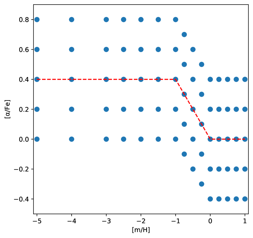
Figure 3: $[\mathrm{\alpha}/\mathrm{Fe}]$ vs. metallicity coverage of the GES synthetic spectra grid. The red dashed line shows the MADERA grid coverage used to determine stellar atmospheric parameters and Fe, Al and Ni abundances.

As mentioned previously, the overall metallicity and $[\mathrm{\alpha}/\mathrm{Fe}]$ ratios follow the same relation as Equation 1, but the grid includes extra $[\mathrm{\alpha}/\mathrm{Fe}]$ enrichments at each metallicity, as illustrated in Figure 3. The spectral resolution of the GES synthetic spectra have been degraded in order to match that of the observational data ($R\sim 7\,500$) with a binning of $0.35\,$Å.

In order to get the $[\mathrm{\alpha}/\mathrm{Fe}]$ abundance ratios, we follow the analogous procedure as in Section 4.2: we create a 1D grid $S2_{i}(\lambda)=S(\hbox{$[\mathrm{\alpha}/\mathrm{Fe}]$}_{i},\lambda)$ by trilinear interpolation from the eight neighboring grid points of the GES 4D grid of synthetic spectra to the calibrated MADERA stellar atmospheric parameters $\hbox{$T_{\mathrm{eff}}$}_{\rm,DR6}$, $\hbox{$\log g$}_{\rm DR6}$, and $\hbox{$[{\rm m}/{\rm H}]$}_{\rm DR6}$ of the underlying Rave star. The initial $[\mathrm{\alpha}/\mathrm{Fe}]$ of the input spectrum is assumed to follow Equation 1. A 1D grid with 9 elements is then created by applying the analogous interpolation to atmospheric parameters sets with $\hbox{$[\mathrm{\alpha}/\mathrm{Fe}]$}=\hbox{$[\mathrm{\alpha}/\mathrm{Fe}]$}_{\rm initial}\pm 0.1$, $\hbox{$[\mathrm{\alpha}/\mathrm{Fe}]$}_{\rm initial}\pm 0.2$, $\hbox{$[\mathrm{\alpha}/\mathrm{Fe}]$}_{\rm initial}\pm 0.3$, and $\hbox{$[\mathrm{\alpha}/\mathrm{Fe}]$}_{\rm initial}\pm 0.4$, respectively, but keeping $T_{\mathrm{eff}}$, $\log g$, and $[{\rm m}/{\rm H}]$ unchanged. We then compute the quadratic distance between the observed spectrum $S(\lambda)$ and each of the interpolated synthetic spectra of $S2_{i}(\lambda)$ over the whole spectral range. We exclude the cores of the Ca II triplet lines as they can suffer from deviations owing to NLTE effects or chromospheric emission lines depending on the spectral type. An example of such a 1D grid is shown in Figure 4, for a Rave spectrum.

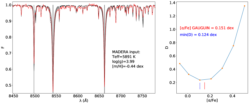
Figure 4: Example of $[\mathrm{\alpha}/\mathrm{Fe}]$ ratio measurement via GAUGUIN for the target 20070423_1650m57_114, with MADERA input. Grey zones are avoided in the fit (Ca II cores). The left hand panel shows, in black, the set of synthetic spectra interpolated to the stellar atmospheric parameters of the star, with 7 values of $[\mathrm{\alpha}/\mathrm{Fe}]$. The observed spectrum is shown in red. The right-hand panel displays the distance between the models and the observed spectrum, as a function of the $[\mathrm{\alpha}/\mathrm{Fe}]$ of each synthetic spectrum. The rough minimum of the quadratic distance (blue dashed line) is refined by the Gauss-Newton algorithm, leading to a different minimum (red line) and hence abundance. We notice that in this case only 7 models are use for the distance computation because of the grid edge effect in this metallicity regime.

For both steps, derivation of the elemental abundances of Al, Ni and Fe, as well as for the $\alpha$ overabundance, a rough minimum of the quadratic distance is given by the closest point to the true minimum (see Figure 4, right panel, dashed line). It is then refined using a Gauss-Newton algorithm (Bijaoui et al., 2012), as illustrated by the red dashed line in Figure 4. We provide a $\chi^{2}$ fit between the observed spectrum and a synthetic one, computed for the GAUGUIN abundance solution.

GAUGUIN was implemented combining C++ and IDL, allowing it to derive $60$ $[\mathrm{\alpha}/\mathrm{Fe}]$ ratios per second, and $1\,200$ individual abundances per second. For the analysis of the whole data set with GAUGUIN (normalization, abundances + errors) the overall computation time was 29 hours, on a single CPU-core.

4.4 Calibration of GAUGUIN [Fe/H], [Al/H], [Ni/H] ratios

The synthetic spectra adopted to derive [Fe/H], [Al/H], [Ni/H] ratios are calibrated with respect to the Sun and verified with respect to Arcturus and Procyon (Kordopatis et al., 2011; Kordopatis, 2011). From line-to-line, small mismatches can occur between the observed Solar and Arcturus spectra and their respective synthetic spectrum. We therefore chose to apply a zero-point correction to the GAUGUIN abundances. To do so, we determined with GAUGUIN the chemical abundances for the Sun and Arcturus, using the high resolution library of Hinkle et al. (2003), degraded to match the Rave  spectral resolution. The input stellar atmospheric parameters of both stars were chosen to be consistent with those obtained by MADERA. The MADERA zero-point correction was derived by feeding GAUGUIN with the un-calibrated stellar atmospheric parameters derived by MADERA from the Solar and Arcturus spectra: Sun {$\hbox{$T_{\mathrm{eff}}$}_{,u}=5\,578\,$K, $\hbox{$\log g$}_{u}=4.09$, $\hbox{$[{\rm m}/{\rm H}]$}_{u}=-0.24\,$dex}; Arcturus {$\hbox{$T_{\mathrm{eff}}$}_{,u}=4\,318$K, $\hbox{$\log g$}_{u}=2.04$, $\hbox{$[{\rm m}/{\rm H}]$}_{u}=-0.35\,$dex}. The averaged zero-point corrections that we apply to the GAUGUIN-derived [Fe/H], [Al/H] and [Ni/H] abundances are presented in Table 3. The $[\mathrm{Fe}/\mathrm{H}]$ corrections are minor as GAUGUIN tends to track the input metallicity very well. Arcturus zero-point abundances have been applied to giants ($\hbox{$\log g$}\leq 3.5$), while the Solar zero-point abundances have been applied to dwarfs ($\hbox{$\log g$}>3.5$), line by line. We note that such zero-point corrections will shift the global patterns in the [X/Fe]$\,vs.\,$$[\mathrm{Fe}/\mathrm{H}]$ plane, but their slope will remain mainly unchanged owing to very small $[\mathrm{Fe}/\mathrm{H}]$ corrections.

Table 3: Zero-point corrections that we added to GAUGUIN $[{\rm X}/{\rm H}]$ abundances, for the giants (Arcturus) and dwarfs (Sun).

Elem.	$\text{Corr}_{\text{Arc}}$	$\text{Corr}_{\text{Sun}}$
Fe	+0.01	+0.02
Al	-0.13	-0.17
Ni	-0.16	-0.19

4.5 Individual errors on [$\alpha$/Fe], [Fe/H], [Al/H] and [Ni/H]

We provide individual error estimates on the GAUGUIN abundance ratios, while for the previous releases only a global error was provided (Kunder et al., 2017). To do so, we considered two main sources of uncertainty: propagation of the errors of the stellar atmospheric parameters $\sigma_{p}(p\pm e_{p})$, and the internal error of GAUGUIN due to noise $\sigma_{\text{int}}(\hbox{SNR})$ (internal precision, see the adopted procedure below). We combined them in a quadratic sum and we obtained the total uncertainty of the GAUGUIN chemical abundances:

$$\sigma=\sqrt{\sigma_{p}^{2}(p\pm e_{p})+\sigma_{\text{int}}^{2}(\hbox{SNR})}.$$ (8)

We detail the way we computed $\sigma_{\text{int}}(\hbox{SNR})$ in the following section.

4.5.1 The precision of GAUGUIN [$\alpha$/Fe], [Fe/H], [Al/H] and [Ni/H] abundances

The top row of Figure 5 presents the internal precision $\sigma_{\text{int}}(\hbox{SNR})$ as a function of SNR for $[\mathrm{\alpha}/\mathrm{Fe}]$, [Al/H], [Fe/H], and [Ni/H], derived by GAUGUIN. The internal precision was characterized by taking 500 measurements of the abundance from noisy synthetic spectra of Sun-like ($\hbox{$T_{\mathrm{eff}}$}=5\,750\,$K, $\hbox{$\log g$}=4.5$, $\hbox{$[{\rm m}/{\rm H}]$}=+0.0$, $\hbox{$[\mathrm{\alpha}/\mathrm{Fe}]$}=+0.0$) and Arcturus-like stars ($\hbox{$T_{\mathrm{eff}}$}=4\,250\,$K, $\hbox{$\log g$}=1.5$, $\hbox{$[{\rm m}/{\rm H}]$}=-0.5$, $\hbox{$[\mathrm{\alpha}/\mathrm{Fe}]$}=+0.3$), adopting $\hbox{SNR}=5$ to $120$, with steps of $\Delta\hbox{SNR}=5$. We computed a simple standard deviation of the 500 abundance measurements, at a given SNR and for a given spectral line. Figure 5 clearly shows that the internal error is larger for dwarf stars than it is for giants. The overall $[\mathrm{\alpha}/\mathrm{Fe}]$ based on the overall fit of the spectrum appears to be pretty robust, with low $\sigma$ (high precision). For [Ni/H] in dwarfs, the internal error varies strongly from one spectral line to another.

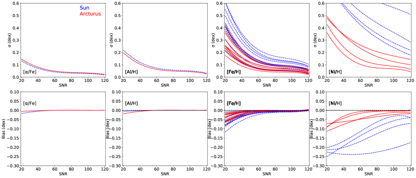
Figure 5: The internal precision (top row) of GAUGUIN and the internal accuracy (bottom row) as a function of Gaussian SNR, for the overall $[\mathrm{\alpha}/\mathrm{Fe}]$ and the individual lines of [Fe/H], [Ni/H], and [Al/H] (one curve per spectral line). The results are given for tests performed on both Solar-like stars (blue, dashed lines) and Arcturus-like stars (red, full lines).

4.5.2 The accuracy of GAUGUIN [$\alpha$/Fe], [Fe/H], [Al/H] and [Ni/H] abundances

We investigate the ability of GAUGUIN to determine accurate abundances in the presence of noise. We adopt the same strategy as in Section 4.5.1, measuring abundances in synthetic spectra of Arcturus- and Sun-like stars. The bottom panel of Figure 5 shows the bias as the difference between the average over 500 measurements of $[{\rm X}/{\rm H}]$ by GAUGUIN and the expected abundance, for individual lines. For a typical giant like Arcturus, we see that the bias tends naturally to be zero for $\hbox{SNR}>50$, except for some Ni lines which tend to settle around a bias of $0.03\,$dex at high SNR. For a Sun-like star, the bias behaves very well for Fe for $\hbox{SNR}>40$. For both stars, GAUGUIN creates no systematics for [Al/H], even at very low SNR, the single spectral line being unblended and strong even in the Sun. On the other hand, in a Sun-like star, Ni exhibits large systematics with respect to Fe and Al because of its weak spectral lines. We conclude that our GAUGUIN-derived values intrinsically do not suffer from large systematics. We point out that in dwarfs, [Ni/H] values should be treated with caution, and can suffer from large systematics, even at large SNR.

4.5.3 Total uncertainty of GAUGUIN [$\alpha$/Fe], [Fe/H], [Al/H] and [Ni/H] abundances

Figure 6 shows the total uncertainty of the GAUGUIN $[\mathrm{\alpha}/\mathrm{Fe}]$, [Fe/H], [Al/H], [Ni/H] ratios, derived using Equation 8, using MADERA stellar atmospheric parameters as input. We show only stars with a quality flag equal to ”0” (as described in Section 3.1.1). We observe that while the total uncertainties of $[\mathrm{\alpha}/\mathrm{Fe}]$ abundances are very similar between dwarfs and giants ($\sim 0.16\,$dex), the total uncertainties of the other abundances are systematically larger for dwarfs.

When discarding stars with $\hbox{SNR}<40$, we tend to remove the tail towards larger errors of the distributions. The typical errors for giants are of the order of $0.13\,$dex for Fe and Al, and $>0.2\,$dex for Ni. We give the median errors of each distribution in Table 4. We note that even at high SNR, Ni suffers from larger uncertainties for dwarf stars. We strongly recommend the reader to use the individual total errors in order to select the most reliable GAUGUIN abundances for their specific science application.

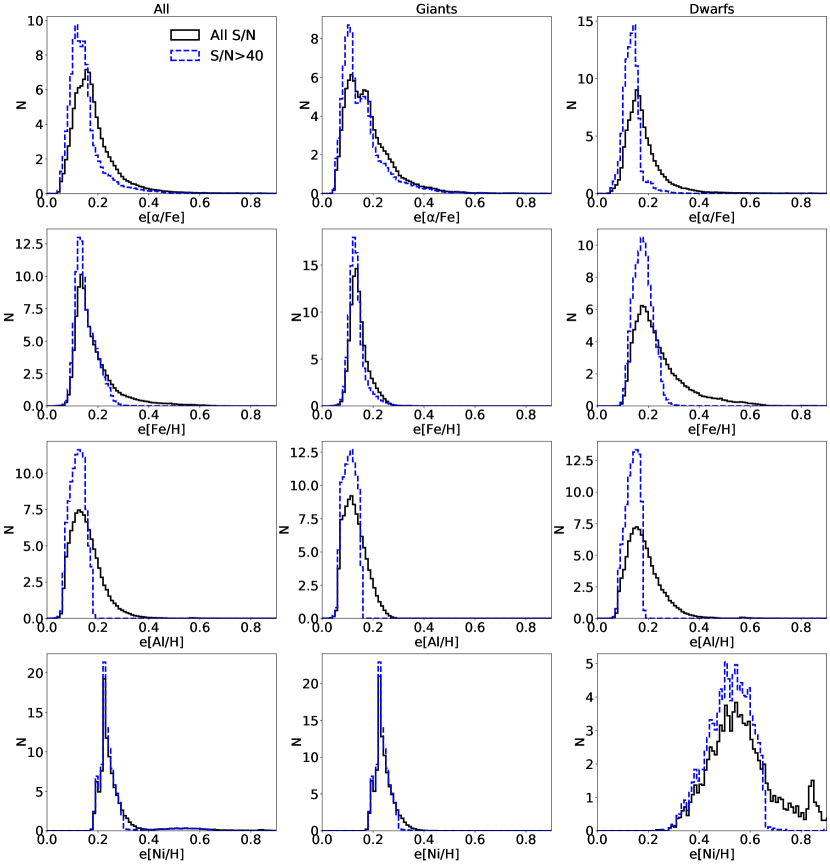
Figure 6: The distribution of total uncertainties for the $[\mathrm{\alpha}/\mathrm{Fe}]$ ratios measured by GAUGUIN, with MADERA input. Left: whole sample. Middle: giants ($\log g<3.5$). Right: dwarfs ($\log g\geq 3.5$).

Elem	SNR	All	Giants	Dwarfs
$[\mathrm{\alpha}/\mathrm{Fe}]$	all	0.16	0.16	0.17
	$>40$	0.13	0.13	0.13
$[$Fe/H$]$	all	0.16	0.14	0.21
	$>40$	0.14	0.13	0.18
$[$Al/H$]$	all	0.14	0.12	0.17
	$>40$	0.12	0.11	0.14
$[$Ni/H$]$	all	0.24	0.23	0.56
	$>40$	0.23	0.23	0.52

Table 4: Total GAUGUIN error for all elements, in the whole sample, giants and dwarfs, respectively. The error is presented adopting MADERA inputs. We refer the reader to Figure 6 for a view of the distribution.

4.5.4 Further sources of uncertainty

We conclude this discussion by testing the sensitivity of GAUGUIN-derived abundances to micro-turbulence, rotational velocity, and radial velocity.

• Micro-turbulence ($\xi$) is included in the GES synthetic spectra grid used by GAUGUIN, following a calibrated relation based on $T_{\mathrm{eff}}$, $\log g$, and $[{\rm m}/{\rm H}]$. Tests based on synthetic spectra revealed that the error on the GAUGUIN $[\mathrm{\alpha}/\mathrm{Fe}]$ due to an error of $1\,\hbox{$\mathrm{km\,s}^{-1}$}$ in $\xi$ is of the order of $0.01$ dex for both Arcturus-like and Solar-like stars. For individual [Fe/H], [Al/Fe], [Ni/H], this error reaches 0.02 dex, i.e. much smaller than the accuracy limit given by the resolution and SNR limit of the RAVE spectra (typically 0.15-0.20 dex uncertainty on chemical abundances). The effects of micro-turbulence on the chemical abundances published in DR6 are thus negligible.

• We investigate how stellar rotation affects the GAUGUIN $[\mathrm{\alpha}/\mathrm{Fe}]$ ratios, as such physical effects are not included in GAUGUIN or MADERA. We measure $[\mathrm{\alpha}/\mathrm{Fe}]$, Fe, Al, and Ni in the synthetic spectra of two Arcturus- and Solar-like stars, for which we convolved the spectra with increasing rotational velocities (from 1 to 10 $\mathrm{km\,s}^{-1}$). Our tests reveal that such neglect of rotation is reasonable, as the induced systematic errors on the $[\mathrm{\alpha}/\mathrm{Fe}]$ are only of the order of $0.009-0.017\,$dex for a typical rotational velocity of $5\,\hbox{$\mathrm{km\,s}^{-1}$}$. This error is only of the order of $0.01-0.02\,$dex for [Fe/H], [Al/H], and [Ni/H]. As before, most of the RAVE stars should fall well below this limit.

• We tested the sensitivity of GAUGUIN when the observed spectrum and the set of synthetic spectra are not in the same rest-frame. The typical accuracy of Rave’s RV is $<2\,\hbox{$\mathrm{km\,s}^{-1}$}$, corresponding to $16\%$ of a pixel. We perform the test on synthetic spectra of the Sun and Arcturus, and estimate that the error on our four abundances due to such a shift in the “observed” spectrum leads to errors of the order of $0.015\,$dex for both spectral types. We note that this error is negligible at high SNR, but tends to increase by a factor of two for $\hbox{SNR}<40$. In this regime we expect larger uncertainties in the RV determination, and for RV errors of 4-5 $\mathrm{km\,s}^{-1}$, the uncertainty on GAUGUIN abundances increases by a factor of two. We encourage the reader to filter stars with large RV uncertainties, as mentioned in Sect 6.

4.6 Sample selection and quality of fit

The internal error analysis presented above intrinsically assumes that the morphology of the observed Rave spectrum matches that of the synthetic grid. However, this condition does not necessarily need to be fulfilled, for example owing to a peculiarity of the Rave spectrum, either of an astrophysical nature (e.g., significantly deviant abundance pattern of the underlying star or shortcomings of the synthetic grid, particularly in the less studied ranges of the parameter space), or for technical reasons (improper continuum normalization e.g., owing to fringing).

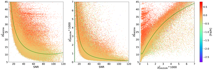
Figure 7: Left: $\chi^{2}$ values vs. SNR for the MADERA pipeline. The green line corresponds to the median values as approximated by Equation 9. The distribution is color coded by the metallicity $[{\rm m}/{\rm H}]_{\rm DR6}$. Middle: $\chi^{2}$ values vs. SNR for the $[\mathrm{\alpha}/\mathrm{Fe}]$ determination with the GAUGUIN pipeline. The green line corresponds to the median values as approximated by Equation 10. The distribution is color coded by the metallicity $[{\rm m}/{\rm H}]_{\rm DR6}$. Right: $\chi^{2}$ for the MADERA and GAUGUIN pipeline plotted against each other.

The quality of the match between an actual Rave spectrum and the synthetic grids employed by the MADERA and GAUGUIN pipeline can be characterized by the two $\chi^{2}$ values provided by the MADERA and GAUGUIN pipelines (see also Figure 7): A poor match of the MADERA pipeline will result in large residuals between the Rave and the template spectrum, which in turn will result in a poor fit of GAUGUIN and/or in excessive (and likely unphysical) deviation in $[\mathrm{\alpha}/\mathrm{Fe}]$. In addition, poor SNR will naturally also lead to unreliable determinations using MADERA and/or GAUGUIN.

Figure 7 illustrates this effect by showing, as a function of the SNR and color coded by metallicity $[{\rm m}/{\rm H}]_{\rm DR6}$, the $\chi^{2}_{\rm MADERA}$ (left) and $\chi^{2}_{\rm GAUGUIN}$ value for all objects for which GAUGUIN provides a converged solution for $[\mathrm{\alpha}/\mathrm{Fe}]$. The green line corresponds to the median $\chi^{2}$ as a function of SNR, approximated by the following two relations:

$$\chi^{2}_{{median},{\rm MADERA}}(\hbox{SNR})=\frac{10^{5}}{-1.23\,\hbox{SNR}^{2}+227\,\hbox{SNR}\ +725}$$ (9)

and

$$\chi^{2}_{{median},{\rm GAUGUIN}}(\hbox{SNR})=\frac{1}{0.232\,\hbox{SNR}^{2}+27.7\,\hbox{SNR}\ -302}\qquad,$$ (10)

for $10<\hbox{SNR}<150$. respectively. The right plot shows the $\chi^{2}$ values for MADERA and GAUGUIN against each other. The majority of the data points fall within a smooth distribution around the median value of either pipeline. Furthermore, as indicated by the right plot, usually both pipelines have a comparable quality of fit, i.e. stars for which the MADERA pipeline provides results within the main distribution of the quality of fit also fall within the main distribution for GAUGUIN. However, both pipelines show a sizeable number of stars with considerably poorer fits than average even for very high SNR values, usually associated with (MADERA-derived) very high super-solar metallicity. This is particularly prominent in the results for the MADERA pipeline. This finding is not very surprising as the aforementioned outliers predominantly correspond to very cool stars with a very dense forest of absorption lines, often also based on molecular lines, i.e. where the proper modeling of synthetic spectra and the matching to medium resolution medium SNR data is particularly challenging.

A simple and convenient way to characterize the simultaneous fit of GAUGUIN and MADERA can be defined via

$$\hbox{$\bar{\chi}^{2}$}=\mu_{\rm MADERA}\,\frac{\chi^{2}_{\rm MADERA}}{\chi^{2}_{{median},\rm MADERA}(\hbox{SNR})}+\mu_{\rm GAUGUIN}\frac{\chi^{2}_{\rm GAUGUIN}}{\chi^{2}_{{median},\rm GAUGUIN}(\hbox{SNR})},$$ (11)

with $\mu_{\rm MADERA}$ and $\mu_{\rm GAUGUIN}$ being being two arbitrary weighing factors. $\bar{\chi}^{2}$ is basically an effective $\chi^{2}$ for the combined fit, and its inverse, i.e., $Q=1/\hbox{$\bar{\chi}^{2}$}$ can be seen as a quality parameter, i.e., a low value of $\bar{\chi}^{2}$ (a high value of $Q$) corresponds to a good fit. For the following we assume $\mu_{\rm MADERA}=1.25$ and $\mu_{\rm GAUGUIN}=1$, i.e. we are a bit more restrictive with respect to the quality of the MADERA metallicity because of the poorer fits for some of the metal-rich stars.

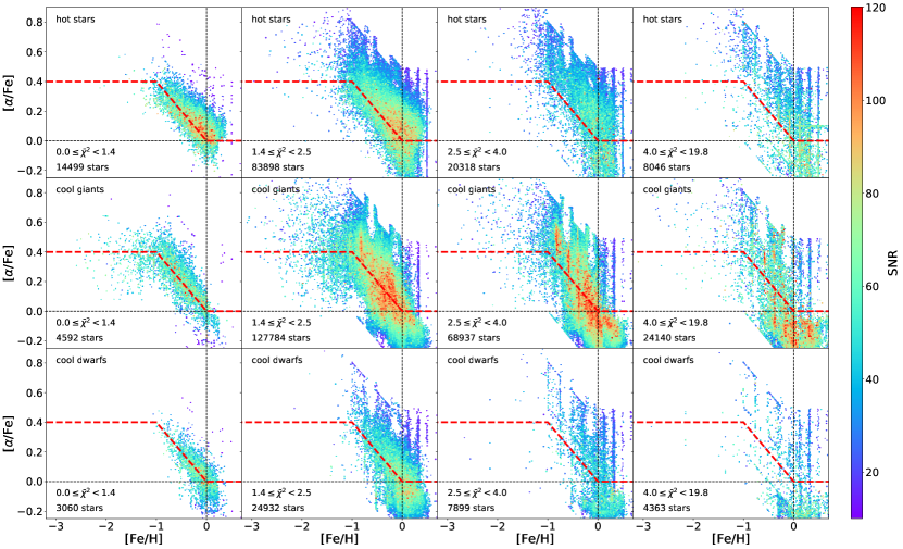
Figure 8: $[\mathrm{\alpha}/\mathrm{Fe}]$ vs. iron as a function of SNR and the quality of the fit. The top row shows hot stars ($\hbox{$T_{\mathrm{eff}}$}>5500$ K), the middle row cool giants ($\hbox{$T_{\mathrm{eff}}$}\leq 5500$ K, $\hbox{$\log g$}<3.5$), the lower row cool dwarfs ($\hbox{$T_{\mathrm{eff}}$}\leq 5500$ K, $\hbox{$\log g$}\geq 3.5$). The four columns from left to right show subsamples with a successively poorer quality parameter $\bar{\chi}^{2}$ of the GAUGUIN and MADERA fit (i.e., successively higher values). The color coding corresponds to the SNR of the spectrum.

In Figure 8 we consider the $[\mathrm{\alpha}/\mathrm{Fe}]$ vs. iron relation for 4 different bins in the quality parameter $\bar{\chi}^{2}$, namely $0\leq\hbox{$\bar{\chi}^{2}$}<1.4$, $1.4\leq\hbox{$\bar{\chi}^{2}$}<2.5$, $2.5\leq\hbox{$\bar{\chi}^{2}$}<4$, and $\hbox{$\bar{\chi}^{2}$}\geq 4$. The ($[\mathrm{Fe}/\mathrm{H}]$,$[\mathrm{\alpha}/\mathrm{Fe}]$) values are color-coded by SNR. We separate the population of stars into three categories based on the BDASP stellar parameters, hot stars ($\hbox{$T_{\mathrm{eff}}$}\ >5500$ K, top row), cool giants ($\hbox{$T_{\mathrm{eff}}$}\ >5500$ K and $\hbox{$\log g$}<3.5$, middle row), and cool dwarfs ($\hbox{$T_{\mathrm{eff}}$}\ >5500$ K and $\hbox{$\log g$}>3.5$, bottom row).

The high quality ($\hbox{$\bar{\chi}^{2}$}<1.4$) sample shows the expected behavior: for metallicities above ${\hbox{$[\mathrm{Fe}/\mathrm{H}]$}}\approx-1$, all stars follow the $[\mathrm{\alpha}/\mathrm{Fe}]$ vs $[\mathrm{Fe}/\mathrm{H}]$ relation of the Galactic disk. Owing to the scatter in the abundance determination of about 0.15 dex even for the highest quality sample, a separation into two disk components cannot obviously be seen (see, however, section 8.1). Cool dwarfs, which owing to their low luminosity are mainly in the immediate neighborhood of the Sun, mainly have abundances comparable to the Sun, hot stars that can be identified to larger distances extend the $[\mathrm{\alpha}/\mathrm{Fe}]$ vs. $[{\rm m}/{\rm H}]$ relation towards considerably lower abundances. For cool giants, the data extends well into the metal poor regime $\hbox{$[{\rm m}/{\rm H}]$}<-1$, and the transition to a constant $\alpha$ overabundance is nicely traced. Relaxing the quality criteria keeps these characteristics at first for all three populations, but increases the scatter. For the high SNR end of the distribution, fairly confined and well defined relations can still be traced. A further relaxation of the quality parameter ($\hbox{$\bar{\chi}^{2}$}>2.5$) results in populating the area near the edges of the GES grid, in particular for the lower SNR data.

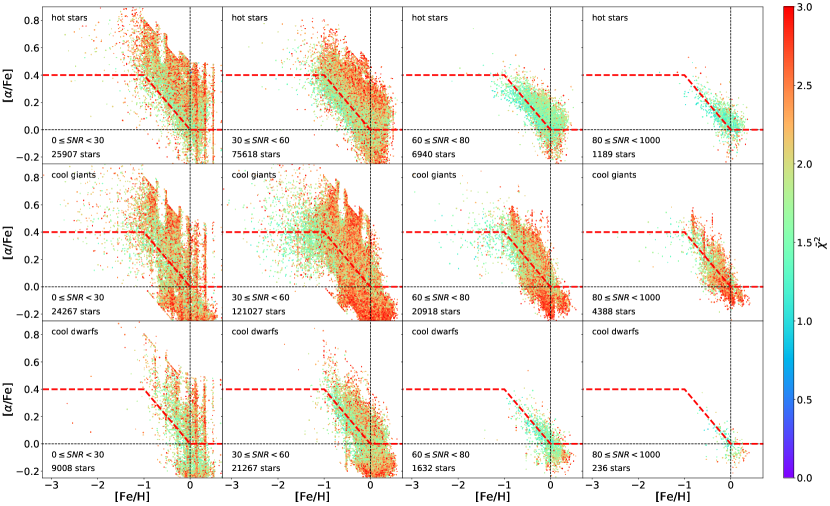
Figure 9: Same as Figure 8 but columns representing bins with increasing SNR (from left to right). The color coding corresponds to the $\bar{\chi}^{2}$ value of the fit.

The aforementioned behavior is also reflected in Figure 9, which illustrates it, now projected in bins of different SNR (and color coding by $\bar{\chi}^{2}$). In particular, it shows a systematic shift of the $[\mathrm{\alpha}/\mathrm{Fe}]$ vs. $[\mathrm{Fe}/\mathrm{H}]$ relation with decreasing SNR, with the lower SNR subset seeming to have systematically higher $[\mathrm{\alpha}/\mathrm{Fe}]$. This effect can be understood, as the pipeline reacts to the increasing noise level by interpreting this as a higher $\alpha$ abundance. Again this effect is more pronounced in situations where the match between the Rave spectrum and template is poorer.

Overall, $\hbox{$\bar{\chi}^{2}$}<2.5$ provides satisfactory results for hot stars, while for cooler stars and low SNR still some clustering at the grid boundaries, in particular at fairly negative $[\mathrm{\alpha}/\mathrm{Fe}]$ and high metallicity, can be observed. Such a quality cut also removes most targets from the first year of Rave observations that were still contaminated by light from 2nd order spectra (see DR6-1, Section 2.4). The residual presence of questionable abundance measurements at negative $[\mathrm{\alpha}/\mathrm{Fe}]$ and high metallicity can be suppressed by requiring a more stringent (lower) $\bar{\chi}^{2}$ value in particular for lower SNR values. For example, the constraint $\hbox{$\bar{\chi}^{2}$}<1.4$ for $\hbox{SNR}<40$ basically removes all stars with $\hbox{$[\mathrm{\alpha}/\mathrm{Fe}]$}<-0.1$ at $\hbox{$[\mathrm{Fe}/\mathrm{H}]$}>-0.4$. This is demonstrated in Figure 10, in which a critical threshold of $\hbox{$\bar{\chi}^{2}$}<\hbox{$\bar{\chi}^{2}$}_{\rm crit}=1.1\times\sqrt{\hbox{SNR}/10-1.5}$ is applied.

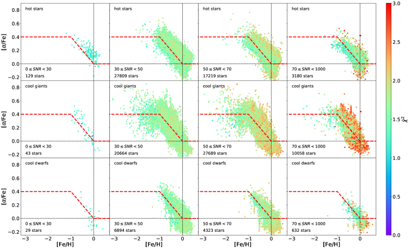
Figure 10: Same as Figure 9 but only stars that fulfill the quality criterion in Equation 11 are shown.

5 Orbits

For the convenience of users of Rave  DR6 we provide the kinematic and orbital properties corresponding to each observed star (see also Table 12 in Sec. 7.5 for a list of the derived quantities). In each case we use as input the position on the sky and proper motion found by Gaia DR2, the radial velocity found by SPARV, and the BDASP derived distance. We take the quoted uncertainty on distance, along with the radial velocity error given as hrv_error_sparv. The proper motion uncertainties are found by summing in quadrature the quoted Gaia uncertainties and an estimate of their systematic uncertainties (66 $\mu{\rm as}\,{\rm yr}^{-1}$, estimated from the small-scale spatially varying measured proper motions of quasars by Lindegren et al., 2018).

Heliocentric positions and velocities are given in the standard coordinate system used in the solar neighborhood, i.e., the X direction is towards the Galactic center ($l=0,b=0$), the Y axis is in the direction of Galactic rotation ($l=90^{\circ},b=0$), and the Z axis points at the north Galactic pole ($b=90^{\circ}$).

The orbital properties are found in the best-fitting Milky Way potential from McMillan (2017). The Sun is assumed to lie at $R_{0}=8.21\,{\rm kpc}$, where the circular velocity is $233.1\,{\rm km}\,{\rm s}^{-1}$ and at a height above the plane $z_{0}=0.014\,{\rm kpc}$ (Binney et al., 1997). The velocity of the Sun with respect to the local standard of rest is taken from Schönrich, Binney, & Dehnen (2010). We place the Sun at $\phi=0^{\circ}$ in our Galactocentric coordinate system, which (combined with the requirement that z increases towards the north Galactic pole) means that the Sun and stars of the Galactic disk have negative $v_{\phi}$, and therefore negative angular momentum around the Galaxy model’s symmetry axis. We note that since this potential is axisymmetric, the orbital parameters we derive are increasingly untrustworthy as the influence of the Galactic bar becomes more significant (e.g., within the bar’s corotation radius, now thought to be of the order $5$ to $6\,{\rm kpc}$ from the Galactic center: Sormani et al., 2015; Portail et al., 2017; Sanders et al., 2019)

The quoted values are derived as a Monte Carlo integral over the uncertainties. Many of the orbital properties have the unfortunate characteristic that a finite change in one of the measured quantities produces an infinite change in the orbital property (since a finite change in position and/or velocity can put the star on an unbound orbit which would have, for example, infinite radial action or apocentric radius), meaning that the expectation (mean) value is inevitably infinite. For this reason we describe the output of the Monte Carlo integral in terms of the median value and the difference between the median and the percentiles corresponding to $\pm 1\sigma$ (i.e. $15.9$ and $84.1$ percent) such that one can quote, for example, the energy as ${\tt Energy}^{+{\tt EnergyPlus}}_{-{\tt EnergyMinus}}$.

The values are found using the GalPot software (Dehnen & Binney, 1998), and the orbital actions $J_{r},J_{z}$ are found using the Stäckel Fudge (Binney, 2012) as packaged in agama (Vasiliev, 2019) – the third action $J_{\phi}$ is the same as the quoted value of the angular momentum.

6 Validation of Rave  DR6 parameters

The data product of large surveys like Rave is always a compromise between the quality of the individual data entry and the area and depth of the survey. This applies to design decisions (like the applied exposure time/targeted SNR) as well as to the decision which data to keep in the sample and which ones to exclude. Our policy for Rave is to provide the maximum reasonable data volume possible, which allows the user to consider the tails of the distribution function. The exact choice of the (sub)sample used for a particular case has to be made by the user based on the criteria needed for the respective science application! Here, we only can give some first guidelines/recommendations regarding the selection of proper sub samples. For a description of the various parameters in the following paragraph we refer to the tables in Section 6 of DR6-1 and Section 7 in this publication.

1. Radial Velocities: Stars with $\texttt{correlationCoeff}>10$ have a small scatter in the repeat measurements of their heliocentric radial velocity. The distribution peaks near $0.0\,$$\mathrm{km\,s}^{-1}$, and the tail toward very large velocity differences is reduced by 90% compared to the uncut sample, indicative of a high confidence measurement (see, e.g., Kordopatis et al., 2013a, and Section 6 of DR6-1). We refer to the data set defined by these criteria as the core sample, or RV.

2. Stellar atmospheric parameters: As a minimum requirement, the quality flags algo_conv_madera of the MADERA pipeline (see Section 3.1.1) should be $\neq 1$, additionally to the aforementioned criteria for the RV measurement. Higher confidence parameters (at the expense of a reduction in sample size) can be obtained by additionally requiring algo_conv_madera$\neq 2$, or even algo_conv_madera$=0$, by requiring that stellar spectra are classified as a certain type and/or by imposing constraints on the SNR.

3. Abundances: basically the same considerations apply here as for the stellar atmospheric parameters, but in addition a quality cut of $\hbox{$\bar{\chi}^{2}$}\lesssim 2.5$ should be applied, with a possibly even stronger constraint for targets with low SNR.

For the stellar parameter and abundance validation against external sources in this and the following section, we define five samples:

• Full: The full set of the Rave DR6 data base for which the pipelines deliver a result.

• RV: The subset of the full data base that fulfills the basic quality criterion for radial velocities (see above and DR6-1 Section 6).

• MD: The subset of the RV data base that fulfills the basic quality criterion for stellar parameter determination with the MADERA pipeline, i.e., $\mathtt{algo\_conv\_madera}\neq 1$.

• BD: The subset of the MD data base that has Gaia DR2 distances and for which BDASP stellar atmospheric parameters could be derived.

• Q_low: The subset of the MD data base that fulfills the basic quality criterion $\hbox{$\bar{\chi}^{2}$}<2.5$ for elemental abundance determination with the GAUGUIN pipeline.

• Q_high: The subset of the MD data base that fulfills the basic quality criterion $\hbox{$\bar{\chi}^{2}$}<\hbox{$\bar{\chi}^{2}$}_{\rm crit}(\hbox{SNR})$ (see Section 4.6) for elemental abundance determination with the GAUGUIN pipeline.

Figure 11 shows the number of objects in $I$ magnitude bins of $0.1$ (left) and the fraction of 2MASS targets in the respective magnitude bin (right) that have an corresponding Rave measurement, for each of these samples. In the bright magnitude bin of Rave ($9<I<10)$, about 55% of the 2MASS targets have a reliable RV measurement in Rave, about 50% have reliable stellar atmospheric parameters, and about 20% (15%) have an $[\mathrm{\alpha}/\mathrm{Fe}]$ estimate in the Q_low (Q_high) sample.

Where additional SNR constraints are added (e.g., to show the Kiel diagram for different SNR cuts in the next subsection), the lower limit of the SNR is added to the sample name. For example, MD40 is the subset of the RV data base that fulfills the basic quality criterion for stellar parameter determination with the MADERA pipeline and for which the individual spectra have a SNR (snr_med_sparv, defined as the inverse of the median of the error spectrum – see Section 3.2 of DR6-1) of at least 40.

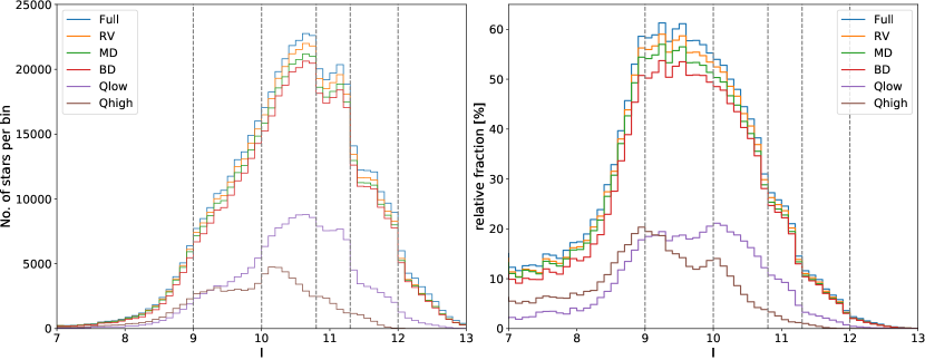
Figure 11: Left: histogram of number of objects per $I$ magnitude bins of $0.1$ for the various Rave DR6 samples as defined at the beginning of Section 6. The magnitude range used per field plate exposure are indicated with dashed lines (see DR6-1, Section 2.2). Right: completeness fraction of the respective sample relative to the number of 2MASS stars, as a function of $I$ magnitude.

The number of spectra and unique objects for the aforementioned samples are given in Table 5 and Table 6, respectively. Dwarfs and giants are divided based on their BDASP $\log g$ values, i.e., $\hbox{$\log g$}_{\rm BDASP}\leq 3.5$ for giants and $\hbox{$\log g$}_{\rm BDASP}>3.5$ for dwarfs.

Table 5: Rave subsamples (spectra) used in this publication for validation and first science applications.

Sample	RV	MADERA	BDASP	$[\mathrm{\alpha}/\mathrm{Fe}]$	Fe	Al	Ni
Full	518,387	517,821	494,695	430,142	328,317	315,036	66,778
RV	497,828	497,708	477,827	425,948	324,856	312,645	65,651
MD	480,254	480,254	460,749	410,873	313,605	302,423	64,136
BD	460,749	460,749	460,749	401,927	307,301	296,096	63,389
– dwarfs			199,047	169,792	97,737	106,510	2,746
– giants			261,702	232,135	209,564	189,586	60,643
Qlow	166,867	166,867	162,646	166,867	122,663	127,864	15,291
– dwarfs				92,446	57,530	65,700	1,286
– giants				70,200	62,080	58,882	13,834
Qhigh	121,812	121,812	118,737	121,812	106,110	106,146	24,042
– dwarfs				59,725	46,015	48,908	1,451
– giants				59,012	57,459	54,575	22,314

Table 6: Rave subsamples (unique objects) used in this publication for validation and first science applications.

Sample	RV	MADERA	BDASP	$[\mathrm{\alpha}/\mathrm{Fe}]$	Fe	Al	Ni
Full	451,783	451,358	431,060	380,319	292,196	281,379	61,824
RV	436,340	436,249	418,485	376,912	289,203	279,337	60,742
MD	423,021	423,021	405,524	365,117	280,205	271,112	59,371
BD	405,524	405,524	405,524	357,161	274,565	265,432	58,686
– dwarfs			173,514	150,487	87,205	95,476	2,572
– giants			232,147	206,788	187,429	170,010	56,118
Qlow	153,634	153,634	149,781	153,634	113,188	118,223	14,596
– dwarfs				84,502	52,563	60,266	1,196
– giants				65,311	57,857	54,973	13,239
Qhigh	110,768	110,768	107,995	110,768	96,558	96,805	22,286
– dwarfs				53,905	41,510	44,338	1,327
– giants				54,112	52,683	50,071	20,707

6.1 Kiel diagrams of the Rave DR6 catalog

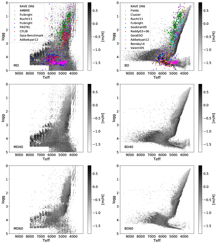
Figure 12: Kiel diagrams for MADERA (left) and BDASP (right) for various SNR levels. In the top row, the calibration sample is overplotted, color coded by the origin as given by the key in the plot.

Figure 12 shows the Rave sample defined by the different quality cuts in the $T_{\mathrm{eff}}$ vs $\log g$ plane (the “Kiel diagram”), where the blue scale is coded by the metallicity $[{\rm m}/{\rm H}]$. The quality cuts applied are (from top to bottom) for the left column (i) the MD sample, (ii) the MD40 sample, and (iii) MD60 sample, while for the right column, (i) the BD sample, (ii) the BD40 sample, and (iii) BD60 sample is shown, respectively. In the top left frame (MADERA), the stellar atmospheric parameters of the calibration sample are also plotted, color coded by their origin (see Appendix A). In the top right frame (BDASP) we also show the validation sample used below for verifying the output of the GAUGUIN pipeline.As one can see, calibration and validation samples nicely cover the most relevant areas of the Kiel diagram, namely the main sequence, turn-off stars and subgiants, and the giant branch and red clump region. For the Ruchti et al. (2011) sample, which was designed as a follow-up study of low metallicity candidates drawn from earlier Rave data releases, the shift towards higher temperature when compared to the higher-metallicity Gaia-ESO DR5 sample is clearly visible, a feature that is nicely reproduced for the MADERA and BDASP pipelines. Furthermore, the pixelization of the MADERA pipeline (for a discussion see DR4, Section 6.3) is clearly visible.

The results for the BDASP pipeline show a considerable sharpening of the distribution, with the main sequence and the position of the red clump being clearly defined. In particular, the region for $\hbox{$\log g$}>3.5$ strongly benefits from the inclusion of Gaia parallaxes, as these dwarf stars are predominantly at lower distances ($d\lesssim 0.8$ kpc) and thus benefit from the accuracy of the parallax measurement.

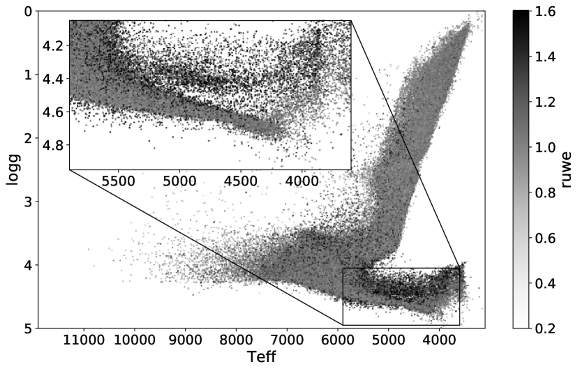
Figure 13: Kiel diagram using the BDASP stellar atmospheric parameters for the BD00 sample, color encoded by the re-normalized unit weight error (RUWE) of the Gaia DR2 astrometric solution.

For higher SNR cuts, a clearly defined sequence nearly parallel to the main sequence but shifted by about +0.2 dex in $\log g$ becomes visible. This parallel sequence is mainly a product of unresolved binaries. These binaries form a second track in the color magnitude diagram, about 0.7 mag brighter than main sequence stars of the same color. BDASP assumes every target to be a single star, and therefore finds a poor match between stars on this track and main sequence stars, instead finding close matches with pre-main-sequence stars which have lower $\log g$ at the same $T_{\mathrm{eff}}$. This explanation can be given more credence by the following observation: In Figure 13 we color code the Kiel diagram by Gaia’s re-normalized unit weight error (RUWE, Lindegren, 2018), which is an indication of the quality of the Gaia DR2 astrometric fit. We see that the RUWE is noticeably higher in the parallel sequence, which is consistent with the astrometry being perturbed by the binary motion of the stars.

We can both illustrate and verify the automated classification scheme (see Section 4 in DR6-1) by showing where stars of different classifications lie in the $\log g$ vs $T_{\mathrm{eff}}$ plane (Figure 14): The classification scheme nicely shows the transition to hot stars above a temperature of $\hbox{$T_{\mathrm{eff}}$}\approx 7000\,$K owing to the presence of strong Paschen line features, which dominate over the Ca triplet feature. On the main sequence, at effective temperatures below $5000\,$K, chromospheric emission lines become more prevalent in these cool and active stars (Žerjal et al., 2013). At temperatures below $4000\,$K, molecular lines lead to a classification of the star as cool or as having carbon features, in particular near the tip of the giant branch. A slightly pinkish color in the sequence parallel to the main sequence for temperatures above 4500 K also indicates a binary origin of stars in this part of the $\log g$ vs $T_{\mathrm{eff}}$ plane, for temperatures below 4500 K, the emission line characteristics dominates the classification also in this part of the parallel sequence.

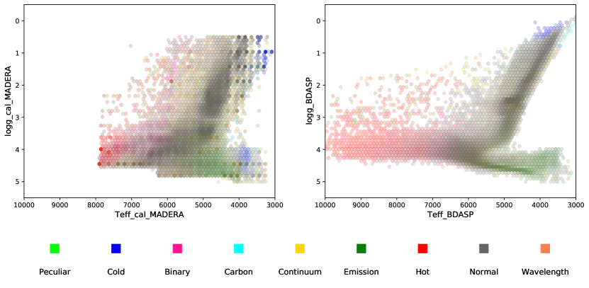
Figure 14: Kiel diagrams for MD sample (left) and the BD sample (right) color coded by the automated classification of the stars.

6.2 Validation against external observations

6.2.1 Validation of stellar atmospheric parameters

For an extensive validation of the pure spectroscopic MADERA stellar atmospheric parameters and their limitations we refer to the DR4 and DR5 publications.

Figure 15 compares $T_{\mathrm{eff}}$, $\log g$, and $[{\rm m}/{\rm H}]$ derived from each of the MADERA and BDASP pipelines for the MD20 and BD20 sample with the values derived from 1094 external high-resolution observations (see appendix A). For the BDASP sample, the metallcity $[{\rm M}/{\rm H}]$ has been scaled to $[{\rm m}/{\rm H}]$ using the inverse of equation 5. Note that this comparison is not fully independent, as some of the external data set has been used to calibrate the outcome of the MADERA pipeline (see Section 3.1, Appendix A). The effective temperatures of both methods give similar results in terms of uncertainties. However, the MADERA pipeline is more affected if low SNR Rave targets are included in the comparison (for the MD00 sample, the standard deviation for MADERA increases to 320K, while the value for BDASP remains basically unchanged). A closer inspection of the MADERA plot also reveals a tendency to somewhat overestimate the temperatures between $5000$ and $6000$ K by $\approx 250$ K. This becomes more visible when the MADERA $T_{\mathrm{eff}}$ are compared with the temperatures derived via the infrared flux temperatures (see Figure 16). As expected, no such trend is visible in the effective temperature of the BDASP pipeline, which has used $T_{\mathrm{eff,IRFM}}$ as an input value.

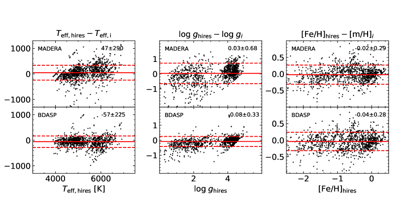
Figure 15: Comparison of the residual (defined as high-resolution observation minus Rave DR6) of the stellar parameter pipelines MADERA (top row) and BDASP (bottom row) against the value of the given stellar parameter derived from the high-resolution data. Left column: $T_{\mathrm{eff}}$, middle column: $\log g$, right column: $[{\rm m}/{\rm H}]$ (for MADERA and BDASP) and $[\mathrm{Fe}/\mathrm{H}]$ (for validation data), respectively. The solid red line indicates the average residual, the dashed red lines show the $\pm 1\sigma$ deviation and the corresponding values are shown in the upper right corner of each frame.

The surface gravities $\log g$ demonstrate the full potential of the parallax constraint from Gaia DR2. The derivation of $\log g$ has always be a major challenge for Rave because of the short wavelength interval and well known degeneracies (Kordopatis et al., 2011). The MADERA pipeline results for $\log g$ are on average unbiased, but exhibit a scatter of about 0.68 dex, while the BDASP pipeline can considerably reduce the uncertainty to only 0.33 dex and produce $\log g$ values that are unbiased, compared to asteroseismic estimates (see Section 6.4). Indeed, a comparison of the structure of the $\log g$ vs $T_{\mathrm{eff}}$ diagram with external data from the GALAH and APOGEE surveys (Section 6.3), plus the analysis of the repeat observations in Section 6.5 below, and the comparison with the asteroseismic information (Section 6.4) all lead to the conclusion that as far as $\log g$ is concerned, much of the variation between the values obtained with BDASP and the external measurements may well need to be attributed to uncertainties in the external calibration sample.

In terms of the metallicity $[{\rm m}/{\rm H}]$, both pipelines perform equally well, and indeed we recommend using the MADERA $[{\rm m}/{\rm H}]$ as the metallicity estimate, as it is the only one that is directly derived spectroscopically.

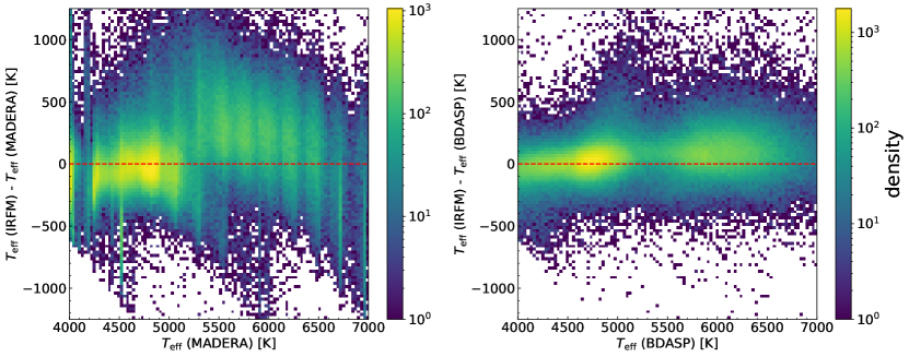
Figure 16: Comparison between the effective temperatures derived from the IRFM against those obtained with MADERA (left panel) and BDASP (right panel), for the MD20 sample. For MADERA, giants with $\hbox{$T_{\mathrm{eff}}$}<5200$ K have temperatures that agree well with IRFM temperatures, but there is a systematic offset for main-sequence/turnoff stars. The pixelization, an artifact of the Rave  stellar parameter pipeline MADERA, is apparent as vertical bands. The BDASP pipeline, which uses $T_{\mathrm{eff,IRFM}}$ as input, shows no significant systematic offsets.

6.2.2 Validation of GAUGUIN abundances

$[\mathrm{\alpha}/\mathrm{Fe}]$ ratios

Figure 17 (top row) compares the $[\mathrm{\alpha}/\mathrm{Fe}]$ ratios obtained with GAUGUIN using the stellar atmospheric parameters $T_{\mathrm{eff}}$, $\log g$, and $[\mathrm{Fe}/\mathrm{H}]$ of the calibration sample (see Section 6.2.1 and DR5 Section 7) against the $[\mathrm{\alpha}/\mathrm{Fe}]$ ratios of the calibration sample (defined as the average of [Si/Fe] and [Mg/Fe]). The abundances trace the pattern observed in the external reference stars very well, with a scatter of about 0.12 dex, and almost no bias. The bottom row of Figure 17 shows the analogous comparison when MADERA $T_{\mathrm{eff}}$, $\log g$, and $[{\rm m}/{\rm H}]$ are used as input parameters. The abundances trace the pattern observed in the external reference stars still well, with a scatter somewhat increasing for lower-metallicity stars. Outliers can be directly mapped to large differences in $T_{\mathrm{eff}}$, $\log g$, and $[{\rm m}/{\rm H}]$ between the calibration sample and the corresponding MADERA values. This is consistent with the poor $\bar{\chi}^{2}$ values for those outliers.

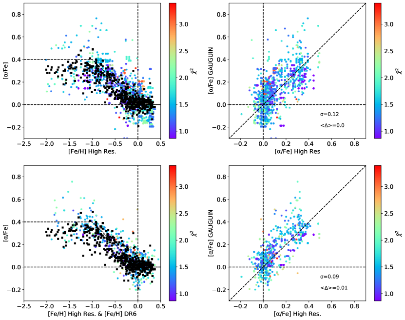
Figure 17: Top row, left panel: GAUGUIN $[\mathrm{\alpha}/\mathrm{Fe}]$ as a function of [Fe/H] (dots, color-codded with $\bar{\chi}^{2}$) computed using the stellar atmospheric parameters of the calibration sample. The black squares correspond to the calibration sample. The right panel plots the $[\mathrm{\alpha}/\mathrm{Fe}]$ ratios obtained with GAUGUIN against those of the calibration sample. Bottom row: same, but using MADERA inputs for computing GAUGUIN $[\mathrm{\alpha}/\mathrm{Fe}]$ ratios. $\Delta$ denotes the difference between the $[\mathrm{\alpha}/\mathrm{Fe}]$ ratios derived via the GAUGUIN pipeline and that derived from high-resolution observations of the reference star. The mean difference and its standard deviation are shown in the bottom right corner of the right column.

The [Fe/H], [Al/H], and [Ni/H] ratios

The top row of Figure 18 compares [Fe/H], [Al/H], and [Ni/H] obtained with the GAUGUIN pipeline against those of the calibration sample. GAUGUIN was fed with the stellar atmospheric parameters of the calibration sample. For [Fe/H], the bias seems to slightly increase towards the [Fe/H]-poor regime, with a dispersion of 0.09 dex. For [Al/H] and [Ni/H] ratios, we notice a weak scatter as well, 0.13 and 0.08, respectively. For [Ni/H] we unfortunately have only very few stars. The biases and scatters observed here can be due to several factors, such as the different linelists and spectral resolution of RAVE and the reference studies.

In the bottom panel of Figure 18, we compare the GAUGUIN [Fe/H], [Al/H], and [Ni/H] values derived with MADERA input to those of the calibration sample (same stars as in the top row). For [Fe/H] and [Al/H], we notice an increase of the scatter for the Fe-poor regime. Basically, the comparison gives fairly satisfactory results, with an increased dispersion, driven by different input stellar atmospheric parameters.

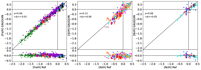
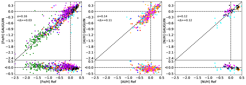
Figure 18: Top: GAUGUIN chemical abundances of [Fe/H], [Ni/H], and [Al/H] computed using calibration sample stellar atmospheric parameters, as a function of the chemical abundances of the calibration sample. We have adopted the same color code for the external sample as was used in Figure 12. $\Delta$ denotes the difference between the abundance of a given element derived via the GAUGUIN pipeline and that derived from high-resolution observations of the reference star. The mean difference and its standard deviation are shown in the upper left corner of each frame. Bottom: same, but using MADERA stellar atmospheric parameters as input for GAUGUIN.

Abundance trends in the Kiel diagram

Abundance trends for the $[\mathrm{\alpha}/\mathrm{Fe}]$, $[\text{Al/Fe}]$ and $[\text{Ni/Fe}]$ can nicely be followed by grouping them by $\log g$ and $T_{\mathrm{eff}}$ in the Kiel diagram. This is done in Figure 19 for $[\mathrm{\alpha}/\mathrm{Fe}]$ and for $[\text{Al/Fe}]$ and $[\text{Ni/Fe}]$ in Figures 20 and 21, respectively. In these diagrams we bin stars of the BD40 sample by their BDASP $\log g$ and $T_{\mathrm{eff}}$ in bins of size 1 dex and 500 K, respectively. We start with $4<\hbox{$\log g$}\leq 5$ and $4000<\hbox{$T_{\mathrm{eff}}$}\leq 4500$ in the lower right panel with $T_{\mathrm{eff}}$increasing towards the left, and $\log g$ decreasing going upwards. The leftmost plot includes all stars hotter than 7000 K. Each panel shows the $[\mathrm{\alpha}/\mathrm{Fe}]$ vs $[\mathrm{Fe}/\mathrm{H}]$ relation, and in addition show an icon of the Kiel diagram in blue, with the respective sub sample marked in red.

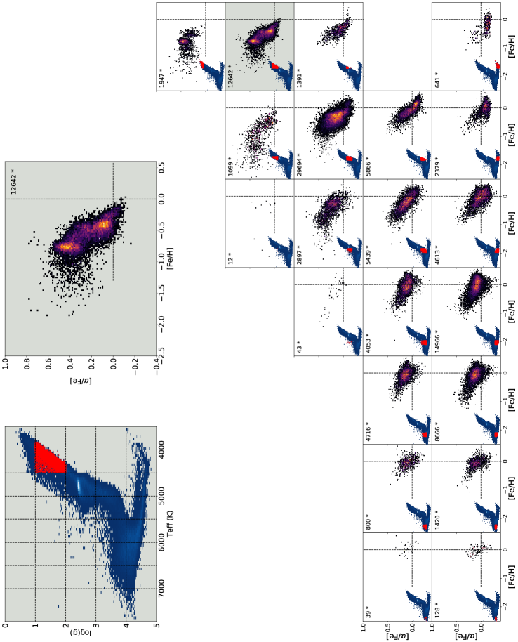
Figure 19: $[\mathrm{\alpha}/\mathrm{Fe}]$ as a function of [Fe/H] for the Q_high sample, binned in $T_{\mathrm{eff}}$ ($\Delta\hbox{$T_{\mathrm{eff}}$}=500\,$K) and $\log g$ ($\Delta\hbox{$\log g$}=1\,$dex). In each panel, we added a Kiel diagram in order to help the reader locating the subsample in the $\hbox{$T_{\mathrm{eff}}$}-\hbox{$\log g$}$ plane. For illustration purposes, the two inlays in the upper left corner magnify the subpanel for $\hbox{$T_{\mathrm{eff}}$}<4500\,$K and $1<\hbox{$\log g$}<2$. In total, $[\mathrm{\alpha}/\mathrm{Fe}]$ and $[\mathrm{Fe}/\mathrm{H}]$ abundances for $103\,474$ stars are shown.

The $[\mathrm{\alpha}/\mathrm{Fe}]$ vs $[\mathrm{Fe}/\mathrm{H}]$ relation across the $T_{\mathrm{eff}}$-$\log g$ plane is shown in Figure 19. The figure nicely demonstrate how the GAUGUIN derived abundances can track the systematically different behavior for different Galactic populations. For giants we probe predominantly the low metallicity regime, which shows a successively increasing $\alpha$ overabundance with decreasing metallicity and the transition to a plateau at $\hbox{$[\mathrm{\alpha}/\mathrm{Fe}]$}\approx 0.4$. Main sequence stars, on the other hand, mainly test the thin disk behavior of the extended solar suburb.

Indeed, while we, as demonstrated in the next section, clearly see several populations of stars in terms of their combined chemical and kinematical properties, only in very few areas in the $T_{\mathrm{eff}}$-$\log g$ plane do we simultaneously see several components, most notably at $\hbox{$T_{\mathrm{eff}}$}<5000$ K and $\hbox{$\log g$}<2$, i.e. for red giants. There is also a trend that the slope of the $\hbox{$[\mathrm{\alpha}/\mathrm{Fe}]$}-\hbox{$[\mathrm{Fe}/\mathrm{H}]$}$-relation is steeper for giants than it is on the main sequence. When comparing these findings with those of other surveys we have to alert the reader to properly take into account the different selection effects. For example APOGEE predominantly focuses on giants and has a large fraction of their targets at low Galactic latitudes (thanks to the NIR nature of this survey), while this area is almost completely excluded by the survey design of Rave. We also note that bright giants are a much rarer population in the Rave sample, reflecting the relatively bright magnitude limit of Rave compared with other ongoing surveys. Rave is basically dominated by two populations, main sequence stars and red clump stars, as indicated by the density scale in Figure 19.

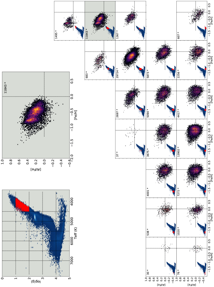
Figure 20: Same as Figure 19, but showing [Al/Fe] as a function of [Fe/H] for the Q_highsample. In total, [Al/Fe] and $[\mathrm{Fe}/\mathrm{H}]$ abundances for $96\,607$ stars are shown.

While not an $\alpha$ element, aluminum is also predominantly formed in massive stars (Thielemann & Arnett, 1985) and released to the ISM via type-II supernovae. Therefore, similar abundance trends as observed for $\alpha$ elements are expected. Indeed, while the scatter is considerably larger - we fit only very few lines in the CaT region, while for $[\mathrm{\alpha}/\mathrm{Fe}]$ we basically make use of the full spectrum - similar trends to those of $\alpha$ elements can be observed (see Figure 20), in particular a relative-to-solar over-abundance of Al for metal-poor giant stars, and a systematic trend of decreasing aluminum abundance for increasing metallicity. For the brightest red giants in our sample, as for $[\mathrm{\alpha}/\mathrm{Fe}]$, only aluminum-enriched very low metallicity stars can be found in the sample, indicative that we trace the halo and metal-weak thick disk component. A kinematical analysis of this subset (see Section 8.2) shows that these stars are indeed on highly eccentric and inclined orbits.

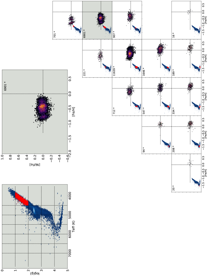
Figure 21: Same as Figure 19, but showing [Al/Fe] as a function of [Fe/H] for the Q_highsample. In total, [Ni/Fe] and $[\mathrm{Fe}/\mathrm{H}]$ abundances for $24\,135$ stars are shown.

As an iron group element, we would expect (within the accuracy expected by Rave) nickel to basically follow the same trends as the iron abundance, i.e., $\hbox{$[\mathrm{Ni}/\mathrm{Fe}]$}\approx 0$. This is indeed the case as illustrated by Figure 21, which shows systematic changes in the overall abundance as we move from red giants via red clump stars to main sequence stars, but the relative abundance between Ni and Fe basically remains constant.

6.3 Comparison of Rave  with the APOGEE and GALAH surveys

APOGEE and GALAH are two high-resolution spectroscopic campaigns currently underway. APOGEE has $R=22,500$ resolving power in the NIR, and mainly focuses on giant stars in the Galactic disk. Most of the publicly released APOGEE data cover the Northern hemisphere, so there is little overlap with Rave so far. The joint sample of Rave and APOGEE DR16 (Ahumada et al., 2019) – with the Rave quality constraints defined above and with abundances flagged by the APOGEE consortium as being reliable – amounts to 4859 objects.

GALAH is a high resolution ($R=28,000$) spectroscopic survey at optical wavelengths using the HERMES spectrograph and the 2dF fiber positioner facility at the AAO 3.9m telescope. The GALAH 2nd data release (Buder et al., 2018), published shortly before Gaia DR2, provides stellar atmospheric parameters and abundances for up to 342,682 stars in the Southern Hemisphere. The Rave and GALAH data sets have 21,534 stars in common. Of these, 13,254 stars have a high SNR (snr_med_sparv $\geq 20$) Rave spectrum and a satisfactory quality GALAH spectrum (flag_cannon $=0$). Only these stars are used in the discussion below, with the further requirement that flag_x_fe $=0$ when discussing individual element abundances $[{\rm X}/{\rm H}]$.

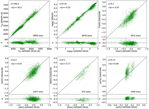
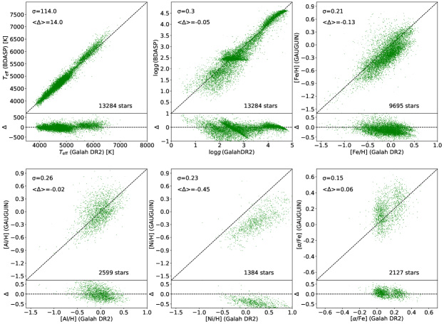
Figure 22: Upper two rows: comparison of the stellar atmospheric parameters and elemental abundances between Rave BDASP and APOGEE DR16, for the stars in common. Lower two rows: Same as the upper panels, but now for the comparisons between Rave BDASP and GALAH DR2. Element abundances for Rave were obtained with the GAUGUIN pipeline using MADERA inputs for $T_{\mathrm{eff}}$ and $\log g$. The number of stars in common is shown in the lower right corner of each panel.

It is illustrative to compare the outcome of the medium resolution Rave data with the considerably higher resolution APOGEE and GALAH data. When performing these comparisons one should, however, be aware that – unlike BDASP – neither the APOGEE nor the GALAH data pipeline has yet made use of the Gaia DR2 parallaxes. However, both surveys employed asteroseismic information from Kepler/K2 for constraining $\log g$.

Figure 22 compares $T_{\mathrm{eff}}$, $\log g$, and the abundances for Fe, Al, Ni, and $\alpha$ between Rave (BDASP) and APOGEE DR16 (upper two rows) and GALAH DR2 (lower two rows). Note that we plot all stars in common, irrespective of their possible classification. This simplification does not affect the general statistics of the comparison samples appreciably, but could be important when comparing individual objects, as discussed in DR6-1, Section 4.

The comparison shows an excellent agreement in the derived values for $\log g$ and $T_{\mathrm{eff}}$. Indeed, the advantage of having Gaia DR2 parallax information available for Rave results in $\log g$ estimates that are at least comparable to those derived with higher resolution spectroscopy. We compared Rave results also with new unpublished GALAH values of $\log g$ and $[\mathrm{Fe}/\mathrm{H}]$, which make use of Gaia astrometry. This new information makes the $\log g$ values of both datasets almost identical ($\Delta=0.03$, $\sigma=0.10$) and decreases the iron abundances for GALAH by $\sim 0.1$ dex. For some elements like Fe, Al, and $\alpha$, the trends between Rave and GALAH and between Rave and APOGEE appear qualitatively to be very similar, exhibiting a slight tilt in the residual in the sense that Rave  tends to underestimate abundances for Solar-type stars. Furthermore, unlike the Rave/APOGEE sample, the Rave/GALAH sample includes both dwarfs and giants, with each component having slightly different systematics, visible in a slight bimodality ($\hbox{$[\mathrm{Fe}/\mathrm{H}]$}>0$ vs $\hbox{$[\mathrm{Fe}/\mathrm{H}]$}<0$). Note that the expected modest decrease in $[\mathrm{Fe}/\mathrm{H}]$ derived from GALAH when the surface gravity is constrained astrometrically affects also the abundances of other elements, as [X$/$H]$=$[X$/$Fe]$+$[Fe$/$H]. As a result, the comparison presented in Figure 22 seems rather conservative, with a suggestion that Rave values could show an even better agreement with high resolution surveys when Gaia DR2 results will be used throughout. This is encouraging for future applications on medium resolution data, like those that will come from WEAVE (Dalton et al., 2018), 4MOST (de Jong et al., 2019), or the Gaia RVS spectrometer. Considering the apparent differences between the two high-resolution surveys we feel confident that our pipelines have extracted the maximum possible from the Rave spectra, given the limitation of resolution and SNR.

6.4 Comparison of Rave  stellar atmospheric parameters with asteroseismically calibrated parameters

Figure  23 compares the asteroseismic $\log g$ derived using equation 6 and $\log g$ obtained from the MADERA and BDASP pipelines. This comparison shows the impact of Gaia DR2 parallaxes on the derived stellar atmospheric parameters, which remove the $\log g$-$T_{\mathrm{eff}}$ degeneracy of the atmospheric stellar atmospheric parameters derived using only spectroscopy.

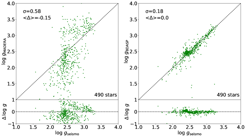
Figure 23: Comparison of the surface gravities $\log g$ derived with the MADERA (left) and BDASP (right) pipeline vs asteroseismically derived values for 490 stars of the K2 campaign.

6.5 Validation with repeat observations

A further way to validate the quality of the Rave data products is to compare the parameters derived for multiple observations of the same object (see Section 2.7 in DR6-1). In the following analysis we calculate for each property $W$ under consideration ($T_{\mathrm{eff}}$, $\log g$, $[\mathrm{\alpha}/\mathrm{Fe}]$, individual element abundances) and for each star $k$ that has $N^{k}_{\mathrm{repeat}}>1$ observations that fulfill the quality threshold, the difference between the observation $i$ ($1\leq i\leq N^{k}_{\mathrm{repeat}}$) derived properties $W_{i}^{k}$ and the mean $\bar{W}^{k}$ for the respective repeat sequence. We then analyze the distribution function of $\Delta W_{i}^{k}=W_{i}^{k}-\bar{W}^{k}$ over all stars $k$ and observations $i$. The distribution function is then approximated by a combination of two Gaussians using a least-squares fit.

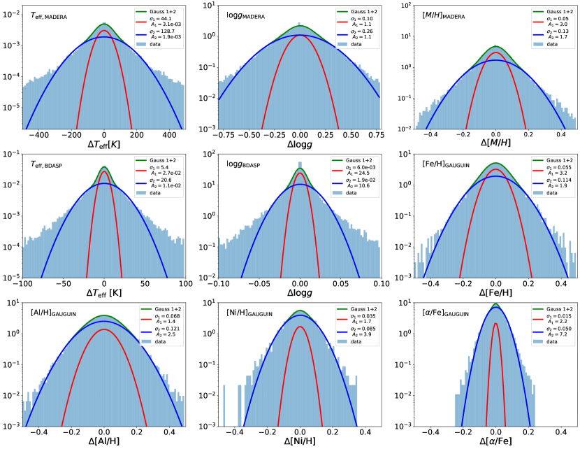
Figure 24: From upper left to lower right: Differences in the MADERA estimated $T_{\mathrm{eff}}$, MADERA estimated $\log g$, MADERA estimated $[{\rm m}/{\rm H}]$, BDASP estimated $T_{\mathrm{eff}}$, BDASP estimated $\log g$  GAUGUIN estimated $[\mathrm{Fe}/\mathrm{H}]$, $[\mathrm{Al}/\mathrm{H}]$, $[\mathrm{Ni}/\mathrm{H}]$, and $[\mathrm{\alpha}/\mathrm{Fe}]$ for stars in the MD20 and BD20 sample with more than one observation, respectively. For the $[\mathrm{\alpha}/\mathrm{Fe}]$ determination, the Q_high cut has been applied.

Figure 24 shows the distribution function for $T_{\mathrm{eff}}$, $\log g$, and the elemental abundances for the MD20/BD20 sample in addition to a fit of the distribution with two Gaussians.

Overall the distributions show very similar behaviour: a core region that is well fit by two Gaussians, plus a wide exponential wing, which includes, however, only a few percent of the overall sample. The prominence of the wing and also the width of the wider Gaussian increases if we move from high (MD40) to lower quality constraint samples (like MD00). Occasionally, a spike at $\Delta W=0$ can be observed, in particular for the MADERA pipeline, reflecting the tendency of this pipeline to assign values close to the vertices of the spectral template grid (“pixelization”). Those spikes are excluded from the fitting procedure.

The distribution for the MADERA values for $T_{\mathrm{eff}}$, $\log g$, and $[{\rm m}/{\rm H}]$, in the repeat sequence gives a result consistent with the differences between the MADERA value and the external data set, though overall the errors appear to be systematically smaller, reinforcing that a considerable uncertainty has to be assumed also for the stellar atmospheric parameters of the high-resolution sample, in particular for $\log g$. The uncertainties for the individual elements are also consistent with the errors quoted in Section 4 and 6.2.2.

The on-first-sight surprisingly small variance in the BDASP values reflects the fact that these properties are predominantly not determined by Rave spectroscopic data. BDASP uses as temperature input $T_{\mathrm{eff,IRFM}}$, which is primarily determined by photometric data (which are the same for all members of a repeat sequence) and only weakly depends on the input $\log g$ from the MADERA pipeline. Variations thus come in only via $[{\rm m}/{\rm H}]$. $\log g$ is mainly determined by Gaia DR2 parallax information in the Bayesian framework, so again only very weakly dependent on the MADERA input and thus on the spectral information.

Table 7: DR6_MADERA catalog description.

Col	Format	Units	NULL	Label	Explanations
1	char	-	N	rave_obs_id	Rave spectrum designation
2	float	K	Y	teff_madera	Effective temperature
3	float	K	Y	teff_cal_madera	Calibrated effective temperature
4	float	K	Y	teff_error_madera	Error in effective temperature
5	float	dex	Y	logg_madera	log surface gravity
6	float	dex	Y	logg_cal_madera	Calibrated log surface gravity
7	float	dex	Y	logg_error_madera	Error in log surface gravity
8	float	dex	Y	m_h_madera	Uncalibrated metallicity $\hbox{$[{\rm m}/{\rm H}]$}_{\rm u}$
9	float	dex	Y	m_h_cal_madera	Calibrated metallicity $\hbox{$[{\rm m}/{\rm H}]$}_{\rm DR6}$
10	float	dex	Y	m_h_error_madera	Error in metallicity $[{\rm m}/{\rm H}]$
11	float	-	Y	algo_conv_madera	Quality flag for MADERA [0..4]
12	float	-	Y	chisq_madera	$\chi^{2}$ of the best fit
13	float	-	Y	snr_madera	SNR  employed in the MADERA pipeline
14	float	-	Y	chisq_madera	$\chi^{2}$ of the best fit

Table 8: DR6_IRFM catalog description.

Col	Format	Units	NULL	Label	Explanations
1	char	-	N	rave_obs_id	Rave spectrum designation
2	float	K	Y	teff_irfm	Temperature from infrared flux method
3	float	K	Y	teff_error_irfm	Internal error on teff_irfm
4	float	mas	Y	rad_irfm	Angular diameter from infrared flux method
5	float	mas	Y	rad_error_irfm	Internal error on rad_irfm_ir
6	char	-	N	method_irfm	IRFM flag

Table 9: DR6_BDASP catalog description. All parameter are determined using the BDASP pipeline.

Col	Format	Units	NULL	Label	Explanations
1	char	-	N	rave_obs_id	Rave spectrum designation
2	float	pc	N	distance_bdasp	Heliocentric distance estimate
3	float	pc	N	distance_error_bdasp	Heliocentric distance uncertainty
4	float	yr	N	age_bdasp	Age estimate
5	float	yr	N	age_error_bdasp	Age uncertainty
6	float	K	N	teff_bdasp	$T_{\mathrm{eff}}$ estimate
7	float	K	N	teff_error_bdasp	$T_{\mathrm{eff}}$ uncertainty
8	float	dex	N	logg_bdasp	$\log g$ estimate
9	float	dex	N	logg_error_bdasp	$\log g$ uncertainty
10	float	$M_{\odot}$	N	mass_bdasp	Mass estimate
11	float	$M_{\odot}$	N	mass_error_bdasp	Mass uncertainty
12	float	-	N	log_a_v_bdasp	Log of extinction ($A_{V}/{\rm mag}$) estimate
13	float	-	N	log_a_v_error_bdasp	Log of extinction ($A_{V}/{\rm mag}$) uncertainty
14	float	dex	N	m_h_bdasp	[M/H] estimate
15	float	dex	N	m_h_error_bdasp	[M/H] uncertainty
16	float	mas	N	parallax_bdasp	Parallax estimate
17	float	mas	N	parallax_error_bdasp	Parallax uncertainty
18	float	mag	N	dist_mod_bdasp	Distance modulus estimate
19	float	mag	N	dist_mod_error_bdasp	Distance modulus uncertainty
20	float	mag	N	a_v_inf_prior_bdasp	Prior on extinction ($A_{V}$) at infinity used

Table 10: DR6_Seismo, the asteroseismically calibrated red giant catalog description.

Col	Format	Units	NULL	Label	Explanations
1	char	-	N	rave_obs_id	Rave spectrum designation
2	float	K	N	teff_seismo	Effective temperature
3	float	K	N	teff_error_seismo	Error in effective temperature
4	float	dex	N	logg_seismo	$\hbox{$\log g$}_{S}$
5	float	dex	N	logg_error_seismo	Uncertainty in $\hbox{$\log g$}_{S}$
6	float	dex	N	m_h_seismo	$\hbox{$[{\rm M}/{\rm H}]$}_{S}$
7	float	dex	Y	m_h_error_seismo	Uncertainty in $\hbox{$[{\rm M}/{\rm H}]$}_{S}$
8	float	dex	Y	fe_h_seismo	$\hbox{$[\mathrm{Fe}/\mathrm{H}]$}_{S}$
9	float	dex	Y	fe_h_error_seismo	Uncertainty in $\hbox{$[\mathrm{Fe}/\mathrm{H}]$}_{S}$
10	float	dex	Y	mg_h_seismo	$\hbox{$[\mathrm{Mg}/\mathrm{H}]$}_{S}$
11	float	dex	Y	mg_h_error_seismo	Uncertainty in $\hbox{$[\mathrm{Mg}/\mathrm{H}]$}_{S}$
12	float	-	Y	chisq_seismo	$\chi^{2}$ of the best fit

Table 11: DR6_GAUGUIN catalog description.

Col	Format	Units	NULL	Label	Explanations
1	char	-	N	rave_obs_id	Rave spectrum designation
2	float	dex	N	alpha_de_gauguin	$[\mathrm{\alpha}/\mathrm{Fe}]$ estimate from GAUGUIN
3	float	dex	N	alpha_fe_error_gauguin	$[\mathrm{\alpha}/\mathrm{Fe}]$ error from GAUGUIN
4	float	-	N	alpha_fe_chisq_gauguin	$\chi^{2}$ of the best fit
6	float	dex	N	fe_h_gauguin	[Fe/H] estimate from GAUGUIN
7	float	dex	N	fe_h_error_gauguin	[Fe/H] error from GAUGUIN
8	int	-	N	fe_h_nl_gauguin	Number of spectral lines used to derive [Fe/H]
9	float	-	N	fe_h_chisq_gauguin	$\chi^{2}$ of the best line fit
10	float	dex	N	al_h_gauguin	[Al/H] estimate from GAUGUIN
11	float	dex	N	al_h_error_gauguin	[Al/H] error from GAUGUIN
12	int	-	N	al_h_nl_gauguin	Number of spectral lines used to derive [Al/H]
13	float	-	N	al_h_chisq_gauguin	$\chi^{2}$ of the best line fit
14	float	dex	N	ni_h_gauguin	[Ni/H] estimate from GAUGUIN
15	float	dex	N	ni_h_error_gauguin	[Ni/H] error from GAUGUIN
16	int	-	N	ni_h_nl_gauguin	Number of spectral lines used to derive [Ni/H]
17	float	-	N	ni_h_chisq_gauguin	$\chi^{2}$ of the best line fit

7 The sixth Rave public data release: catalog presentation II

Rave DR6 spectra and the derived quantities are made available through a data base accessible via doi:10.17876/rave/dr.6/ (for details see paper DR6-1). Since key words and unquoted identifiers are case insensitive, in SQL, in general lower case identifiers are used in the data base. The two main identifiers are rave_obs_id and raveid: the former, rave_obs_id, is the unique identifier denoting the observation of a particular spectrum – the name is a composite of the observing date, field name, and fiber number allocated to the star on that occasion.

raveid is the unique identifier of the target star, the name being a composite of the targets Galactic coordinates in the J2000.0 system. Consequently, objects that have several observations have the same raveid for all, but differ in their rave_obs_id.

For convenience we also provide a set of FITS, CSV, and HDF files of the overall Rave catalog, featuring key variables sufficient for the majority of applications of the Rave survey. These data are organized in 16 files according to the pipeline employed; the content for 10 of these files is briefly described in the following paragraphs and associated tables, for the remaining 6 we refer to paper DR6-1. We avoid duplication of variable entries in the different files, with the exception of rave_obs_id, which can be used to link the contents of the various catalogs.

7.1 Which Rave DR6 data products to use

The detailed use of the Rave DR6 data products and the quality criteria to be applied depend on the particular science case under consideration. A general recommendation can thus not be made. Considering our experience working with Rave data over the past 15 years, and the various tests we performed in particular in the context of this data release, we recommend as a starting point in particular in the context of Galactic dynamics and Galactic archeology applications:

• To use the BDASP values for $\log g$, $T_{\mathrm{eff}}$, and the distance of the star, and the calibrated MADERA value for the overall metallicity $[{\rm m}/{\rm H}]$. In particular BDASP properties are recommended for the identification of subpopulations (dwarfs, giants, red-clump stars).

• For abundance ratios we recommend the $\alpha$-enhancement and Al, Fe, and Ni values derived using GAUGUIN for $\log g$, $T_{\mathrm{eff}}$, and $[{\rm m}/{\rm H}]$ taken from MADERA, as the MADERA/GAUGUIN combination provides an internally consistent pure spectroscopic framework. The use of BDASP derived parameters as input parameters for a determination of the $\alpha$-enhancement $[\mathrm{\alpha}/\mathrm{Fe}]$ should be taken with caution, as it introduces systematic inconsistencies in the templates used for the determination of $[\mathrm{\alpha}/\mathrm{Fe}]$ and the determination of the metallicity.

• For applications where a purely spectroscopically derived stellar parameter is sought for, we recommend the calibrated MADERA values for $\log g$, $T_{\mathrm{eff}}$, and $[{\rm m}/{\rm H}]$, and $\alpha$-enhancements based on MADERA input parameters.

7.2 The Rave  DR6 catalog of stellar atmospheric parameters

Stellar atmospheric parameters are derived using three pipelines and, consequently, assembled in three catalogs: DR6_MADERA (doi:10.17876/rave/dr.6/006, Table 7),
DR6_IRFM (doi:10.17876/rave/dr.6/007, Table 8), and DR6_BDASP (doi:10.17876/rave/dr.6/008, Table 9). DR6_BDASP also provides an improved distance estimate and extinction measure combining Gaia, spectroscopic and photometric data, as well as estimates for the mass and the age of the respective star based on a Bayesian isochrone comparison.

7.3 The Rave DR6 asteroseismically calibrated Red Giant catalog

The asteroseismically calibrated red giant catalog is provided in the DR6_Seismo file (doi:10.17876/rave/dr.6/013), Table 10). We recommend to use DR6_Seismo only for targets that are classfied with $\mathtt{flag1}=$‘n’ and for which the difference between $\hbox{$\log g$}_{S}$ and $\hbox{$\log g$}_{u}$ is less then 0.5 dex.

7.4 The Rave  DR6 catalog of element abundances and $\alpha$ enhancements

The abundances of the non-iron group elements (Al, Fe, and Ni) and of the $\alpha$ enhancement $[\mathrm{\alpha}/\mathrm{Fe}]$ derived with the pipeline GAUGUIN and MADERA input are provided (doi:10.17876/rave/dr.6/009, Table 11). The analogous table for BDASP input (see comment above) can be found in (doi:10.17876/rave/dr.6/010.

For backward compatibility with the DR4 and DR5 data releases, we also provide a file with chemical abundances derived using the CDR pipeline (Boeche et al., 2011) using $T_{\mathrm{eff}}$, $\log g$, and $[{\rm m}/{\rm H}]$ of the MADERA (DR6_CDR_MADERA, doi:10.17876/rave/dr.6/011) and BDASP (DR6_CDR_BDASP, doi:10.17876/rave/dr.6/012) pipeline as input, but in general recommend the use of elemental abundances from the GAUGUIN pipeline.

7.5 The Rave  DR6 catalog of orbits

DR6_Orbits (doi:10.17876/rave/dr.6/014, Table 12) contains information on the orbits of the Rave stars, obtained under the assumption of a given Milky Way mass model (Section 5).

The Rave DR6 data release is complemented by two files cross-matching Rave DR6 with Gaia DR2 (DR6_GaiaDR2, doi:10.17876/rave/dr.6/015) and with a suite of other catalogs including Tycho-2, 2MASS, WISE, APASS9, and SKYMAPPER (DR6_XMatch, doi:10.17876/rave/dr.6/016).

Table 12: DR6_Orbits catalog description.

Col	Format	Units	NULL	Label	Explanations
1	char	-	N	rave_obs_id	Rave target designation
2	float	kpc	N	helio_x	Heliocentric X position
3	float	kpc	N	helio_x_plus	– positive uncertainty
4	float	kpc	N	helio_x_minus	– negative uncertainty
5	float	kpc	N	helio_y	Heliocentric Y position
6	float	kpc	N	helio_y_plus	– positive uncertainty
7	float	kpc	N	helio_y_minus	– negative uncertainty
8	float	kpc	N	helio_z	Heliocentric Z position
9	float	kpc	N	helio_z_plus	– positive uncertainty
10	float	kpc	N	helio_z_minus	– negative uncertainty
11	float	${\rm km}\,{\rm s}^{-1}$	N	helio_vx	Heliocentric velocity in X direction
12	float	${\rm km}\,{\rm s}^{-1}$	N	helio_vx_plus	– positive uncertainty
13	float	${\rm km}\,{\rm s}^{-1}$	N	helio_vx_minus	– negative uncertainty
14	float	${\rm km}\,{\rm s}^{-1}$	N	helio_vy	Heliocentric velocity in Y direction
15	float	${\rm km}\,{\rm s}^{-1}$	N	helio_vy_plus	– positive uncertainty
16	float	${\rm km}\,{\rm s}^{-1}$	N	helio_vy_minus	– negative uncertainty
17	float	${\rm km}\,{\rm s}^{-1}$	N	helio_vz	Heliocentric velocity in Z direction
18	float	${\rm km}\,{\rm s}^{-1}$	N	helio_vz_plus	– positive uncertainty
19	float	${\rm km}\,{\rm s}^{-1}$	N	helio_vz_minus	– negative uncertainty
20	float	kpc	N	galcyl_r	Galactocentric cylindrical radius
21	float	kpc	N	galcyl_r_plus	– positive uncertainty
22	float	kpc	N	galcyl_r_minus	– negative uncertainty
23	float	kpc	N	galcyl_z	Height above the Galactic plane
24	float	kpc	N	galcyl_z_plus	– positive uncertainty
25	float	kpc	N	galcyl_z_minus	– negative uncertainty
26	float	deg	N	galcyl_phi	Galactocentric azimuth
27	float	deg	N	galcyl_phi_plus	– positive uncertainty
28	float	deg	N	galcyl_phi_minus	– negative uncertainty
29	float	${\rm km}\,{\rm s}^{-1}$	N	galcyl_vr	Velocity in Galactocentric cylindrical radial direction
30	float	${\rm km}\,{\rm s}^{-1}$	N	galcyl_vr_plus	– positive uncertainty
31	float	${\rm km}\,{\rm s}^{-1}$	N	galcyl_vr_minus	– negative uncertainty
32	float	${\rm km}\,{\rm s}^{-1}$	N	galcyl_vz	Velocity perpendicular to the Galactic plane
33	float	${\rm km}\,{\rm s}^{-1}$	N	galcyl_vz_plus	– positive uncertainty
34	float	${\rm km}\,{\rm s}^{-1}$	N	galcyl_vz_minus	– negative uncertainty
35	float	${\rm km}\,{\rm s}^{-1}$	N	galcyl_vphi	Velocity in Galactocentric azimuth
36	float	${\rm km}\,{\rm s}^{-1}$	N	galcyl_vphi_plus	– positive uncertainty
37	float	${\rm km}\,{\rm s}^{-1}$	N	galcyl_vphi_minus	– negative uncertainty
38	float	kpc	N	min_galcyl_r	Minimum Galactocentric cylindrical radius on orbit
39	float	kpc	N	min_galcyl_r_plus	– positive uncertainty
40	float	kpc	N	min_galcyl_r_minus	– negative uncertainty
41	float	kpc	N	max_galcyl_r	Maximum Galactocentric cylindrical radius on orbit
42	float	kpc	N	max_galcyl_r_plus	– positive uncertainty
43	float	kpc	N	max_galcyl_r_minus	– negative uncertainty
44	float	kpc	N	max_galcyl_z	Maximum height above the Galactic plane on orbit
45	float	kpc	N	max_galcyl_z_plus	– positive uncertainty
46	float	kpc	N	max_galcyl_z_minus	– negative uncertainty
47	float	kpc	N	min_galsph_r	Minimum Galactocentric spherical radius on orbit
48	float	kpc	N	min_galsph_r_plus	– positive uncertainty
49	float	kpc	N	min_galsph_r_minus	– negative uncertainty
50	float	kpc	N	max_galsph_r	Maximum Galactocentric spherical radius on orbit
51	float	kpc	N	max_galsph_r_plus	– positive uncertainty
52	float	kpc	N	max_galsph_r_minus	– negative uncertainty
53	float	kpc	N	mean_galcyl_r	Orbit averaged Galactocentric cylindrical radius
54	float	kpc	N	mean_galcyl_r_plus	– positive uncertainty
55	float	kpc	N	mean_galcyl_r_minus	– negative uncertainty
56	float	${\rm km}^{2}\,{\rm s}^{-2}$	N	energy	Orbital energy
57	float	${\rm km}^{2}\,{\rm s}^{-2}$	N	energy_plus	– positive uncertainty
58	float	${\rm km}^{2}\,{\rm s}^{-2}$	N	energy_minus	– negative uncertainty
59	float	${\rm kpc}\,{\rm km}\,{\rm s}^{-1}$	N	angmom	Angular momentum about Galactic $z$ axis
60	float	${\rm kpc}\,{\rm km}\,{\rm s}^{-1}$	N	angmom_plus	– positive uncertainty
61	float	${\rm kpc}\,{\rm km}\,{\rm s}^{-1}$	N	angmom_minus	– negative uncertainty
62	float	-	N	eccentricity	Eccentricity
63	float	-	N	eccentricity_plus	– positive uncertainty
64	float	-	N	eccentricity_minus	– negative uncertainty
65	float	${\rm kpc}\,{\rm km}\,{\rm s}^{-1}$	N	jr	Radial action
66	float	${\rm kpc}\,{\rm km}\,{\rm s}^{-1}$	N	jr_plus	– positive uncertainty
67	float	${\rm kpc}\,{\rm km}\,{\rm s}^{-1}$	N	jr_minus	– negative uncertainty
68	float	${\rm kpc}\,{\rm km}\,{\rm s}^{-1}$	N	jz	Vertical action
69	float	${\rm kpc}\,{\rm km}\,{\rm s}^{-1}$	N	jz_plus	– positive uncertainty
70	float	${\rm kpc}\,{\rm km}\,{\rm s}^{-1}$	N	jz_minus	– negative uncertainty

8 Science Applications

The following section presents some first science applications for Rave DR6. The main aim here is less to demonstrate particularly new results but rather to demonstrate, using well-established features, the capabilities and limits within the Rave data set for Galactic archeology applications.

8.1 Tomography of the volume probed by Rave

In a first science application we show the changes in the iron abundance, $\alpha$ enhancement, and kinematics throughout the volume probed by the Rave survey (for work with previous data releases, often employing a considerably smaller sample of stars, see, e.g., Williams et al. (2013), Boeche et al. (2013), Kordopatis et al. (2013b), Wojno et al. (2016), Wojno et al. (2018), or Carrillo et al. (2018). We employ the full Q_high sample for giants ($\hbox{$\log g$}<3.5$). BDASP stellar atmospheric parameters and abundances using GAUGUIN with MADERA input are used through this section.

The top row of Figure 25 shows a projection of Rave stars onto the $R$-$Z$ plane of the Galactocentric cylindrical coordinate system. Stars are binned using hexagonal bins of size $0.16$ kpc. The upper left plot shows the clear decrease of the average iron abundance as we move from the Galactic plane to larger heights above the Galactic plane. Simultaneously, the composition becomes more $\alpha$ enriched (second plot from the left). The change in abundances coincides with a change in kinematics: The average tangential velocity decreases (second plot from the right), while the disk is hotter, resulting in a higher radial velocity dispersion $\sigma_{R}$ (rightmost plot). The center plot in the top row shows the Galactocentric radial velocity, exhibiting a mild negative radial velocity gradient, consistent with the finding by Siebert et al. (2011b) using Rave DR3.

The next 5 rows dissect the Milky Way in slices and focus on the distribution in the X-Y plane for each of these slices. The slices are for $Z>1\,$kpc (1st row) and $Z\leq-1\,$kpc (bottom row). In between, slices for $-1<Z\leq-0.2\,$kpc (second row), $-0.2<Z\leq 0.2\,$kpc (third row), and $0.2<Z\leq 1\,$kpc (forth row) are shown, respectively. The shrinking size of the slice in the X-Y plane reflects the double-cone structure of the Rave survey volume, created by the exclusion of low Galactic latitude fields, in particular towards the Galactic center.

Each individual slice for $[\mathrm{Fe}/\mathrm{H}]$, $[\mathrm{\alpha}/\mathrm{Fe}]$, $v_{\phi}$, and $\sigma_{R}$ shows a relatively homogeneous structure, with the changes with Z as presented in the previous paragraph, reflecting the disk like structure of the Milky Way. Only the central three slices exhibit some apparent radial gradient in the iron abundance with the distance from the Sun, an immediate result again of the Rave survey geometry: owing to the double conical layout of the survey volume, stars more distant in the central slices are predominantly from larger heights above the Galactic plane and thus have on average lower abundances than stars in the immediate solar neighborhood. The middle column again shows a mild outward directed radial velocity gradient, indicative of a non-axisymmetric gravitational potential.

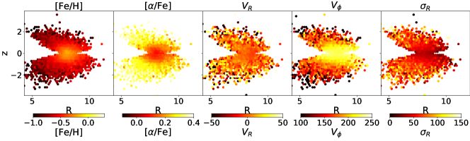
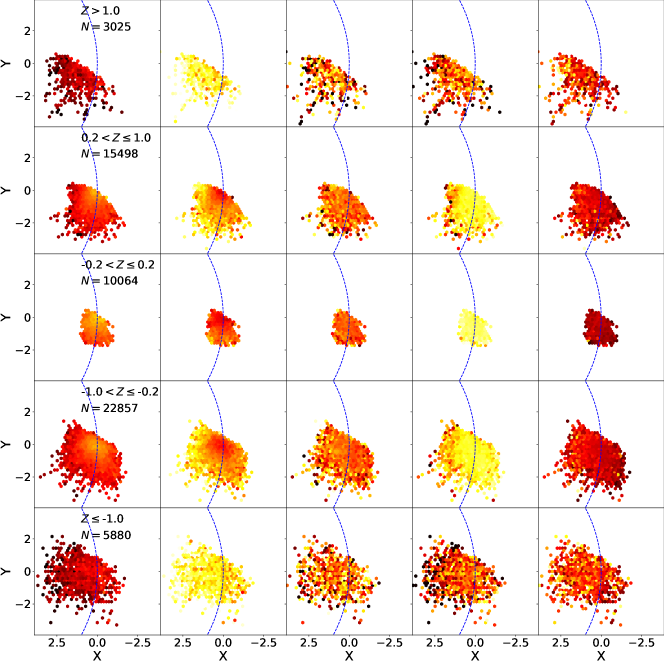
Figure 25: Tomography of the volume probed by Rave. Top row: projection into the Galactocentric R-z plane; next rows from top to bottom: slice in the X-Y plane focused on the local standard of rest (LSR) for stars with $Z>1$ kpc, $0.2<Z\leq 1.0$ kpc, $-0.2<Z\leq 0.2$ kpc, $-1<Z\leq 0.2$ kpc, and $Z\leq-1$ kpc, respectively. The columns show (from left to right) the median of hexbins of size $0.16$ kpc for the iron abundance $[\mathrm{Fe}/\mathrm{H}]$, the $\alpha$-enhancement $[\mathrm{\alpha}/\mathrm{Fe}]$, the Galactocentric radial velocity $V_{R}$, the tangential velocity $|V_{\phi}|$, and the radial velocity dispersion $\sigma_{R}$, respectively. The dotted curve in the X-Y plots indicates the solar circle.

8.2 Relation between chemical abundances and kinematics

In this section we repeat the analysis of Boeche et al. (2013) with the Rave DR6 data set. Unlike Boeche et al. (2013), we, however, only apply a very weak quality cut, namely the full Q_high giant sample with determinations of $[\mathrm{Fe}/\mathrm{H}]$ and $\hbox{$[\mathrm{\alpha}/\mathrm{Fe}]$}=($[Mg/Fe]$+$[Si/Fe]$)/2$. Consequently, the underlying sample could be increased by more than a factor of five from 9,131 in Boeche et al. (2013) to $~{}40,000$ stars, respectively.

As in Gratton et al. (2003) or in Boeche et al. (2013) we begin with a kinematical decomposition into a so-called thin-disk component, dissipative-collapse component and accretion component, based on the eccentricity $e$, the tangential velocity in cylindrical coordinates $V_{\phi}$ and the maximum altitude from the Galactic plane $\text{Z}_{\text{max}}$. The thin-disc component consists of stars with a low eccentricity ($e<0.25$) and low maximum altitude ($Z_{\text{max}}<0.8\,$kpc). The dissipative-collapse component, is composed of stars with higher eccentricity $e>0.25$, traveling higher above the Galactic plane $(\text{Z}_{\text{max}}>0.8\,$kpc), with $V_{\phi}>40\,$$\mathrm{km\,s}^{-1}$. This component is mainly composed of thick disc and halo stars. The accretion component is mainly composed of halo stars and accreted stars. We adopted the criteria $V_{\phi}<40\,$$\mathrm{km\,s}^{-1}$, meaning that such stars are slowly-rotating or even counter-rotating with respect to the Galactic disc. Based on the Q_high sample, we have at hand $39\,130$ stars of the thin disc component, $12\,354$ stars in the dissipative-collapse component, and $1\,931$ stars in the accretion component.

Figure 26 shows the $[\mathrm{\alpha}/\mathrm{Fe}]$ pattern for these three components. The thin-disc component is mainly confined at $\hbox{$[\mathrm{Fe}/\mathrm{H}]$}>-1\,$dex, and shows an increase of its $[\mathrm{\alpha}/\mathrm{Fe}]$ with decreasing $[\mathrm{Fe}/\mathrm{H}]$. The dissipative-collapse component has a large range in iron abundance, with very few metal-rich stars and extends to very low metallicities down to $\hbox{$[\mathrm{Fe}/\mathrm{H}]$}\approx-3\,$dex. Its $[\mathrm{\alpha}/\mathrm{Fe}]$ sequence is narrower, with an increased scatter towards the metal-poor end (owing to halo stars). The accretion component is mostly composed of metal-poor stars, in the range $-2.5<\hbox{$[\mathrm{Fe}/\mathrm{H}]$}<-0.5$, and is $[\mathrm{\alpha}/\mathrm{Fe}]$-rich, but no trend is observed with $[\mathrm{Fe}/\mathrm{H}]$. The thin-disc component is the most metal-rich component ($\langle{\hbox{$[\mathrm{Fe}/\mathrm{H}]$}}\rangle=-0.18\,$dex), while the dissipative-collapse component and the accretion component have an average metallicity of $\langle{\hbox{$[\mathrm{Fe}/\mathrm{H}]$}}\rangle=-0.64\,$dex and $\langle{\hbox{$[\mathrm{Fe}/\mathrm{H}]$}}\rangle=-1.16\,$dex, respectively. The mean $[\mathrm{\alpha}/\mathrm{Fe}]$ increases with decreasing metallicity, i.e., $\langle\hbox{$[\mathrm{\alpha}/\mathrm{Fe}]$}\rangle=+0.11\,$dex for the thin-disc component, $\langle\hbox{$[\mathrm{\alpha}/\mathrm{Fe}]$}\rangle=+0.26\,$dex for the dissipative-collapse component and $\langle\hbox{$[\mathrm{\alpha}/\mathrm{Fe}]$}\rangle=+0.37\,$dex for the accretion component.

In a Toomre diagram, we clearly see that the dissipative-collapse component shows typical kinematics of thick disc stars, but also halo-like kinematics (overlapping with the accretion component). We notice the presence as well of thin-disc like stars belonging to the dissipative-collapse component. The eccentricity increases with decreasing metallicity, and the dissipative-collapse component and the accretion component show considerable overlap (likely due to halo stars). We characterized the gradients of $V_{\phi}$ as a function of $[{\rm m}/{\rm H}]$ in both thin-disc and dissipative-collapse components. In the thin-disc component, we measure a weak anti-correlation ($\nabla=-6\hbox{$\mathrm{km\,s}^{-1}$}/\text{dex}$), while a strong correlation is visible in the dissipative collapse components ($\nabla=+55\hbox{$\mathrm{km\,s}^{-1}$}/\text{dex}$). Such gradients are consistent with previous works, like for example Lee et al. (2011) with SEGUE data or Wojno et al. (2018) for RAVE.

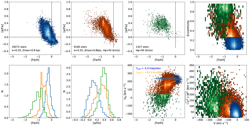
Figure 26: Top row: $[\mathrm{\alpha}/\mathrm{Fe}]$ vs. $[\mathrm{Fe}/\mathrm{H}]$ density maps of the thin-disc component (blue), the dissipative-collapse component (orange), and the accretion component (green). Furthermore the orbital eccentricity is shown against the iron abundance for the three Galactic components. Bottom row: $[\mathrm{Fe}/\mathrm{H}]$ and $[\mathrm{\alpha}/\mathrm{Fe}]$ distributions are shown, complemented by the gradient in the tangential velocity $V_{\phi}$ and the Toomre diagram.

We continue the strategy of Boeche et al. (2013) and analyze the orbits of disk giants in the $\epsilon-Z_{\max}$ plane. We first separate the giant population into 9 different bins with 3 ranges in orbital eccentricity ($0\leq\epsilon<0.2$, $0.2\leq\epsilon<0.4$, and $0.4\leq\epsilon<0.6$) and 3 ranges in maximum altitude, $Z_{\max}$, reached by a star in its orbit ($0\,\mathrm{kpc}\leq Z_{\max}<1\,\mathrm{kpc}$, $1\,\mathrm{kpc}\leq Z_{\max}<2\,\mathrm{kpc}$, and $2\,\mathrm{kpc}\leq Z_{\max}<3\,\mathrm{kpc}$). We then investigate the distributions of the iron abundance $[\mathrm{Fe}/\mathrm{H}]$ (Figure 27), of the $\alpha$ enhancement $[\mathrm{\alpha}/\mathrm{Fe}]$ (Figure 28), and of the tangential velocity $|V_{\phi}|$ (Figure 29), as well as of the mean and minimum Galactocentric cylindrical radius $R_{m}$ and $R_{\min}$ for these 9 bins (Figure 30). Stars on orbits with $\epsilon>0.6$ or $Z_{\max}>3$ kpc are not considered in these plots, as we mainly focus on the thin and thick disk.

We first concentrate on the stars in panel (a), i.e., those on orbits closest to local disk kinematics. Indeed, stars in this bin have a tangential velocity distribution that peaks near 227 $\mathrm{km\,s}^{-1}$, at a mean Galactocentric distance of about 8 kpc. The abundances peak at $\hbox{$[\mathrm{Fe}/\mathrm{H}]$}\approx-0.280$ dex (Figure 27), i.e. somewhat below the solar value and are slightly $\alpha$-enhanced ($\hbox{$[\mathrm{\alpha}/\mathrm{Fe}]$}=0.11$) compared to the immediate solar neighborhood (Figure 28). This reflects the fact that our sample consists of giant stars, which are therefore more distant than a few hundred pc. Indeed, a sample consisting of dwarf stars with the same orbital constraints exhibits a median abundance of $\hbox{$[\mathrm{Fe}/\mathrm{H}]$}=-0.06$ dex and an $\alpha$-enhancement of $\hbox{$[\mathrm{\alpha}/\mathrm{Fe}]$}=0.1$ dex.

As we go from less to more eccentric orbits (panels a $\to$ c) and from lower to higher height above the plane (panels a$\to$ g) or both (panels a$\to$ i), the distribution in the mean orbital radius $R_{m}$ and in particular in the minimum distance $R_{\mathrm{min}}$ becomes broader and more skewed (Figure 30), peaking at considerably smaller Galactocentric cylindrical radii. The median tangential velocity decreases from about 230 $\mathrm{km\,s}^{-1}$ to less than 135 $\mathrm{km\,s}^{-1}$ (panel i) as expected from the increasing asymmetric drift with increasing in velocity dispersion (see previous section). The $[\mathrm{Fe}/\mathrm{H}]$ distribution moves to successively lower values and reaches only $\hbox{$[\mathrm{Fe}/\mathrm{H}]$}\approx-0.75$ in panel i, but the abundance mixture is now considerably more $\alpha$-enriched with $\hbox{$[\mathrm{\alpha}/\mathrm{Fe}]$}\approx 0.34$ (Figure 28), indicating that the sample is increasingly dominated by thick disk and halo stars.

If we focus on the more eccentric orbital bins (c, f, and i), the distribution in velocity and radius is considerably more skewed, as expected, and the metallicity distribution exhibits a tail towards higher abundances (Figure 27). Owing to the high eccentricity, a significant fraction of the stars come from the inner disk, also resulting in a broader distribution in $[\mathrm{Fe}/\mathrm{H}]$, indicating that this is a superposition of at least two populations, a low $[\mathrm{Fe}/\mathrm{H}]$ one with all the chemical characteristics of the thick disk, and a higher $[\mathrm{Fe}/\mathrm{H}]$ one more similar to the inner thin disk. Indeed, Figure 31 shows that while samples with $\hbox{$[\mathrm{Fe}/\mathrm{H}]$}<-0.5$ dex and with $\hbox{$[\mathrm{Fe}/\mathrm{H}]$}>-0.4$ dex have little difference in their respective distribution of $R_{m}$ and $V_{\phi}$, they exhibit quite different patterns in $[\mathrm{\alpha}/\mathrm{Fe}]$, consistent with the findings in Boeche et al. (2013), but now reproduced for a much larger fraction of the Rave DR6 giant sample, as represented by the Q_high sample.

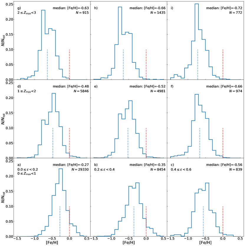
Figure 27: Distribution of iron abundance $[\mathrm{Fe}/\mathrm{H}]$ as a function of orbital parameters: stars are grouped according to their eccentricity $\varepsilon$ (from left to right) and according to their maximum height above the Galactic plane $Z_{\mathrm{max}}$ (from bottom to top). The blue dashed vertical line indicates the median of the distribution, the red dotted line corresponds to the solar value.

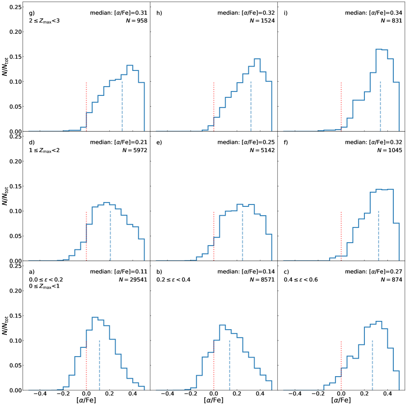
Figure 28: $\alpha$ enhancement $[\mathrm{\alpha}/\mathrm{Fe}]$ for the stellar samples shown in Figure 27. The blue dashed vertical line indicates the median of the distribution, the red dotted line corresponds to the solar value.

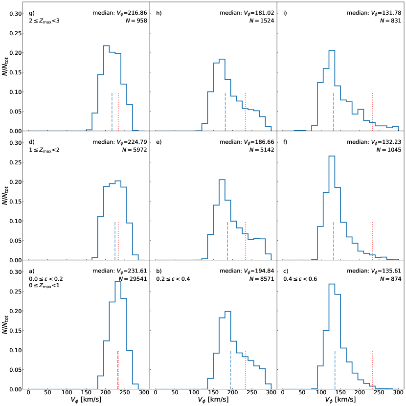
Figure 29: Distribution of tangential velocities $v_{\phi}$ for the stellar samples shown in Figure 27. The blue dashed vertical line indicates the median of the distribution, the red dotted line corresponds to the circular velocity of the LSR.

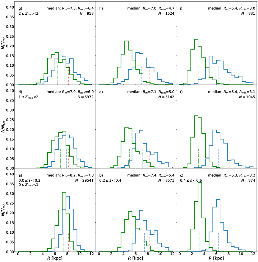
Figure 30: Distribution of the mean Galactocentric cylindrical radius $R_{m}$ (blue) and the minimum Galactocentric cylindrical radius $R_{\mathrm{min}}$ (green) for the stellar samples shown in Figure 27. The blue dashed vertical line indicates the median of the $R_{m}$ distribution, the green dashed-dotted vertical line the median of the $R_{\mathrm{min}}$ distribution, and the red dotted line the radius of the solar circle, respectively.

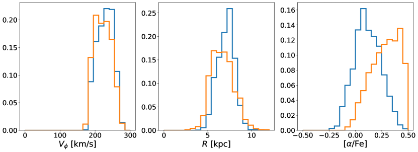
Figure 31: Distribution of $v_{\phi}$, $R_{m}$, and $[\mathrm{\alpha}/\mathrm{Fe}]$ for stars in Figure 27 panel c, separated by those with $\hbox{$[\mathrm{Fe}/\mathrm{H}]$}<-0.5$ dex (blue) and $\hbox{$[\mathrm{Fe}/\mathrm{H}]$}>-0.4$ dex (orange).

We conclude our discussion by taking a tomographic look at the $[\mathrm{\alpha}/\mathrm{Fe}]$ vs. Fe relation and its systematic changes as a function of location in the Galactic disk following the analysis of Hayden et al. (2015), which is based on higher resolution APOGEE data (see, in particular, their Figure 4). Figure 32 shows a similar representation for the RAVE DR6 Q_high giant sample. As we move away from the Galactic plane, we systematically depopulate the high metallicity branch of the disk and start populating the very metal poor and very $\alpha$ enriched region of the $[\mathrm{\alpha}/\mathrm{Fe}]$ vs Fe relation. The respective distributions are, of course, a superposition of the chemical properties of the local environment convolved with that of other regions brought in by stars on highly eccentric and/or highly inclined orbits. Thanks to the astrometry provided by Gaia DR2, we are in the position to disentangle these effects, e.g. rather than plotting the $[\mathrm{\alpha}/\mathrm{Fe}]$ vs $[\mathrm{Fe}/\mathrm{H}]$ relation at the actual position space, by using the average orbital radius (or guiding radius) $R_{m}$ and the maximum height above the Galactic plane ($Z_{\rm max}$) as the respective spatial coordinates (see Figure 33). A comparison with Figure 32 reveals that the stars currently located in the Rave volume are drawn from a considerably larger volume, showing a clear transition from the local disk to the more metal-poor disk at larger heights above the plane to the more halo-type population seen at the largest distances. Also the systematic dependence of metallicity and $\alpha$ enrichment on the eccentricity of the orbit (and/or vice versa) results in clear shifts towards metal poorer and more $\alpha$ enriched populations.

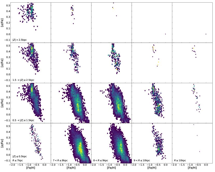
Figure 32: Tomographic plot of the $\alpha$ enhancement $[\mathrm{\alpha}/\mathrm{Fe}]$ vs. $[\mathrm{Fe}/\mathrm{H}]$ of the Q_high sample of $59,012$ giant stars, separated by Galactocentric coordinates $R$ and $Z$.

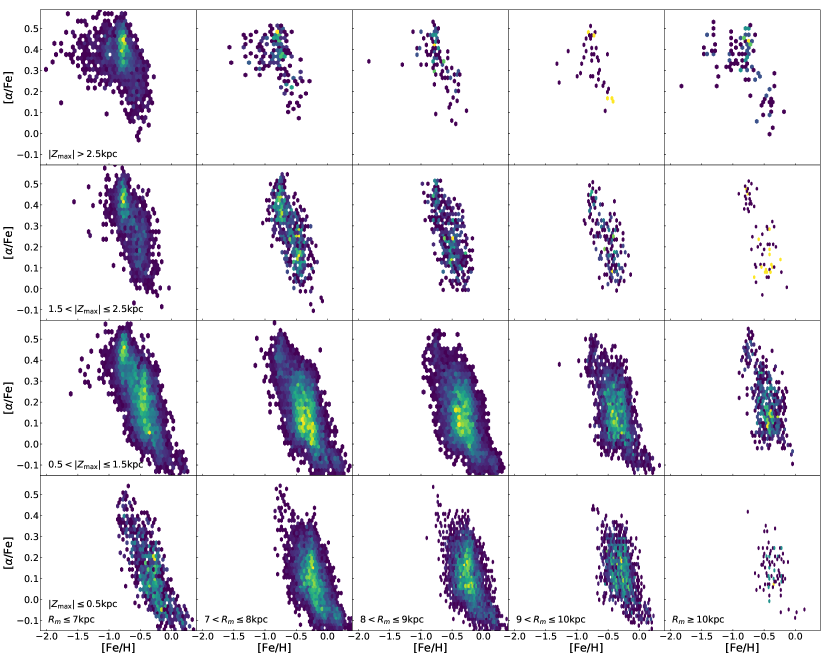
Figure 33: Same as Figure 32, but shown for the mean radius $R_{m}$ and maximum height $Z_{\rm max}$ of the stars orbit, for $58\,985$ giants.

9 Summary and conclusions

The Rave final data release concludes a more-than-15 year effort to provide a homogeneous data set for Galactic archeology studies. Rave DR6 presents spectra and radial velocities for individual stars in the magnitude range $9<I<12$ mag. The spectra cover a wavelength range of $8410-8795\,$Å at an average resolution of $R\approx 7500$. The Rave catalog can be accessed via doi.org/10.17876/rave/dr.6/001. The typical SNR of a Rave star is 40, and the typical uncertainty in radial velocity is $<2$ $\mathrm{km\,s}^{-1}$. For the majority of the 518,387 Rave spectra, reliable atmospheric parameter can be derived with two different pipelines. The MADERA pipeline, based on the algorithms of MATISSE and DEGAS, derives stellar atmospheric parameters purely spectroscopically with uncertainties in $T_{\mathrm{eff}}$, $\log g$, and $[{\rm m}/{\rm H}]$ of 300 K, 0.7 dex, and 0.2 dex, respectively. The Bayesian pipeline BDASP makes use of Gaia DR2 parallaxes, resulting in less-biased $T_{\mathrm{eff}}$ estimates (compared to photometrically derived temperatures with the infrared flux method) for temperatures between $5200-6000$ K and substantially improved estimates of $\log g$ with an uncertainty of about 0.2 dex. BDASP also provides an improved distance estimate and extinction measure combining Gaia, spectroscopic, and photometric data, as well as estimates for the mass and the age of the respective star based on isochrone fitting. The new pipeline, GAUGUIN, provides reliable $\alpha$ enhancements $[\mathrm{\alpha}/\mathrm{Fe}]$ down to low metallicity stars with $\hbox{$[{\rm m}/{\rm H}]$}\lesssim-1$ with an uncertainty of less than $0.2$ dex. Two science applications regarding the chemo-dynamical structure of the volume probed by Rave demonstrate the potential of Rave for applications in the area of Galactic archeology.

Appendix A Calibration and validation samples

As outlined in Section 3.1.2, the output of the MADERA pipeline is calibrated against a sample of reference stars in order to minimize possible systematic effects. The calibration was performed against the stellar atmospheric parameters $T_{\mathrm{eff}}$, $\log g$, and $[{\rm m}/{\rm H}]$, where for the observational data $[\mathrm{Fe}/\mathrm{H}]$ was used as a calibrator. The sample of calibration stars is detailed in Section 4 of Kordopatis et al. (2013a) and Section 6.2 of Kunder et al. (2017). This sample consists of follow-up spectroscopy of (Ruchti et al., 2011) and Fulbright (in preparation), complemented by data in the PASTEL catalog , CFLIB (Valdes et al., 2004) and Gaia benchmark stars of (Jofré et al., 2014). Since not a suitable number of Ravetargets that had literature data available could be identified for the full range of surface gravities, metallicities and effective temperatures, additional high-resolution spectra with coverage of the Rave wavelength range were binned down to Rave-resolution, analyzed with the MADERA pipeline, and added as additional calibration points. This happened as part of the work performed in pervious data releases, in particular DR4 (Kordopatis et al., 2013a). The calibration library consists of in total 1384 spectra covering a broad range of stellar atmospheric parameters in the Kiel diagram (see Figure 12).

For the validation of the chemical abundance pipeline GAUGUIN (and the pipeline by Boeche et al. (2011) for previous data releases), we compiled a list of individual elemental abundances available from high resolution data for stars in the Rave data base. These include data from Ruchti et al. (2011) (383 spectra), Fulbright (in preparation, 178 spectra),Adibekyan et al. (2012) (153 spectra), Reddy et al. (2003) (5 spectra), Reddy et al. (2006) (18 spectra), Soubiran & Girard (2005) (97 spectra), Valenti & Fischer (2005) (72 spectra), Gaia-ESO Gilmore et al. (2012) (71 spectra), and Bensby et al. (2014) (113 spectra), as well as other field (204) and cluster (75) stellar spectra as detailed in Kunder et al. (2017). Since there are a number of common target in the reference data set, the complete validation data set contains 1369 spectra for 948 unique stars. When $[\mathrm{\alpha}/\mathrm{Fe}]$ was given in the respective catalog, this value was adopted, otherwise $[\mathrm{\alpha}/\mathrm{Fe}]$ was estimated from the average of $[\mathrm{Si}/\mathrm{Fe}]$ and $[\mathrm{Mg}/\mathrm{Fe}]$. If only one of the two abundances $[\mathrm{Si}/\mathrm{Fe}]$ and $[\mathrm{Mg}/\mathrm{Fe}]$ as available, this value was used as a proxy for $[\mathrm{\alpha}/\mathrm{Fe}]$.

References

- Adibekyan et al. (2012) Adibekyan, V. Z., Sousa, S. G., Santos, N. C., et al. 2012, A&A, 545, A32, doi: 10.1051/0004-6361/201219401
- Ahumada et al. (2019) Ahumada, R., Allende Prieto, C., Almeida, A., et al. 2019, arXiv e-prints, arXiv:1912.02905. https://arxiv.org/abs/1912.02905
- Alvarez & Plez (1998) Alvarez, R., & Plez, B. 1998, A&A, 330, 1109. https://arxiv.org/abs/astro-ph/9710157
- Andrae et al. (2018) Andrae, R., Fouesneau, M., Creevey, O., et al. 2018, A&A, 616, A8, doi: 10.1051/0004-6361/201732516
- Arenou et al. (2018) Arenou, F., Luri, X., Babusiaux, C., et al. 2018, A&A, 616, A17, doi: 10.1051/0004-6361/201833234
- Asplund et al. (2005) Asplund, M., Grevesse, N., & Sauval, A. J. 2005, in Astronomical Society of the Pacific Conference Series, Vol. 336, Cosmic Abundances as Records of Stellar Evolution and Nucleosynthesis, ed. I. Barnes, Thomas G. & F. N. Bash, 25
- Bailer-Jones et al. (2013a) Bailer-Jones, C. A. L., Andrae, R., Arcay, B., et al. 2013a, A&A, 559, A74, doi: 10.1051/0004-6361/201322344
- Bailer-Jones et al. (2013b) —. 2013b, A&A, 559, A74, doi: 10.1051/0004-6361/201322344
- Bensby et al. (2014) Bensby, T., Feltzing, S., & Oey, M. S. 2014, A&A, 562, A71, doi: 10.1051/0004-6361/201322631
- Bijaoui et al. (2010) Bijaoui, A., Recio-Blanco, A., de Laverny, P., & Ordenovic, C. 2010, in ADA 6 - Sixth Conference on Astronomical Data Analysis, 9
- Bijaoui et al. (2012) Bijaoui, A., Recio-Blanco, A., De Laverny, P., & Ordenovic, C. 2012, Statistical Methodology, 9, 55
- Bijaoui et al. (2012) Bijaoui, A., Recio-Blanco, A., de Laverny, P., & Ordenovic, C. 2012, Statistical methodology, 9, 55
- Binney (2012) Binney, J. 2012, MNRAS, 426, 1324, doi: 10.1111/j.1365-2966.2012.21757.x
- Binney et al. (1997) Binney, J., Gerhard, O., & Spergel, D. 1997, MNRAS, 288, 365, doi: 10.1093/mnras/288.2.365
- Binney et al. (2014) Binney, J., Burnett, B., Kordopatis, G., et al. 2014, MNRAS, 437, 351, doi: 10.1093/mnras/stt1896
- Boeche & Grebel (2016) Boeche, C., & Grebel, E. K. 2016, A&A, 587, A2, doi: 10.1051/0004-6361/201526758
- Boeche et al. (2011) Boeche, C., Siebert, A., Williams, M., et al. 2011, AJ, 142, 193, doi: 10.1088/0004-6256/142/6/193
- Boeche et al. (2013) Boeche, C., Chiappini, C., Minchev, I., et al. 2013, A&A, 553, A19, doi: 10.1051/0004-6361/201219607
- Bressan et al. (2012) Bressan, A., Marigo, P., Girardi, L., et al. 2012, MNRAS, 427, 127, doi: 10.1111/j.1365-2966.2012.21948.x
- Buder et al. (2018) Buder, S., Asplund, M., Duong, L., et al. 2018, MNRAS, 478, 4513, doi: 10.1093/mnras/sty1281
- Burnett & Binney (2010) Burnett, B., & Binney, J. 2010, MNRAS, 407, 339, doi: 10.1111/j.1365-2966.2010.16896.x
- Carrillo et al. (2018) Carrillo, I., Minchev, I., Kordopatis, G., et al. 2018, MNRAS, 475, 2679, doi: 10.1093/mnras/stx3342
- Casagrande et al. (2006) Casagrande, L., Portinari, L., & Flynn, C. 2006, MNRAS, 373, 13, doi: 10.1111/j.1365-2966.2006.10999.x
- Casagrande et al. (2010) Casagrande, L., Ramírez, I., Meléndez, J., Bessell, M., & Asplund, M. 2010, A&A, 512, A54, doi: 10.1051/0004-6361/200913204
- Casagrande et al. (2014) Casagrande, L., Portinari, L., Glass, I. S., et al. 2014, MNRAS, 439, 2060, doi: 10.1093/mnras/stu089
- Cropper et al. (2018) Cropper, M., Katz, D., Sartoretti, P., et al. 2018, A&A, 616, A5, doi: 10.1051/0004-6361/201832763
- Dalton et al. (2018) Dalton, G., Trager, S., Abrams, D. C., et al. 2018, in Society of Photo-Optical Instrumentation Engineers (SPIE) Conference Series, Vol. 10702, Ground-based and Airborne Instrumentation for Astronomy VII, 107021B
- de Jong et al. (2019) de Jong, R. S., Agertz, O., Berbel, A. A., et al. 2019, The Messenger, 175, 3, doi: 10.18727/0722-6691/5117
- de Laverny et al. (2013) de Laverny, P., Recio-Blanco, A., Worley, C. C., et al. 2013, The Messenger, 153, 18
- de Laverny et al. (2012) de Laverny, P., Recio-Blanco, A., Worley, C. C., & Plez, B. 2012, A&A, 544, A126, doi: 10.1051/0004-6361/201219330
- De Silva et al. (2015) De Silva, G. M., Freeman, K. C., Bland-Hawthorn, J., et al. 2015, MNRAS, 449, 2604, doi: 10.1093/mnras/stv327
- Dehnen & Binney (1998) Dehnen, W., & Binney, J. 1998, MNRAS, 294, 429, doi: 10.1046/j.1365-8711.1998.01282.x
- Epchtein et al. (1997) Epchtein, N., de Batz, B., Capoani, L., et al. 1997, The Messenger, 87, 27
- Freeman & Bland-Hawthorn (2002) Freeman, K., & Bland-Hawthorn, J. 2002, ARA&A, 40, 487, doi: 10.1146/annurev.astro.40.060401.093840
- Gaia Collaboration et al. (2016a) Gaia Collaboration, Prusti, T., de Bruijne, J. H. J., et al. 2016a, A&A, 595, A1, doi: 10.1051/0004-6361/201629272
- Gaia Collaboration et al. (2016b) Gaia Collaboration, Brown, A. G. A., Vallenari, A., et al. 2016b, A&A, 595, A2, doi: 10.1051/0004-6361/201629512
- Gaia Collaboration et al. (2018) —. 2018, A&A, 616, A1, doi: 10.1051/0004-6361/201833051
- Gilmore et al. (2012) Gilmore, G., Randich, S., Asplund, M., et al. 2012, The Messenger, 147, 25
- Górski et al. (2005) Górski, K. M., Hivon, E., Banday, A. J., et al. 2005, ApJ, 622, 759, doi: 10.1086/427976
- Graczyk et al. (2019) Graczyk, D., Pietrzyński, G., Gieren, W., et al. 2019, ApJ, 872, 85, doi: 10.3847/1538-4357/aafbed
- Gratton et al. (2003) Gratton, R. G., Carretta, E., Desidera, S., et al. 2003, A&A, 406, 131, doi: 10.1051/0004-6361:20030754
- Grevesse (2008) Grevesse, N. 2008, Communications in Asteroseismology, 157, 156
- Grevesse et al. (2007) Grevesse, N., Asplund, M., & Sauval, A. J. 2007, Space Sci. Rev., 130, 105, doi: 10.1007/s11214-007-9173-7
- Guiglion (2015) Guiglion, G. 2015, PhD thesis, Ecole Doctorale de Sciences Fondamentales et Appliquées, Université Nice Sophia Antipolis - UFR Sciences
- Guiglion et al. (2018a) Guiglion, G., Chiappini, C., Valentini, M., & Steinmetz, M. 2018a, Research Notes of the American Astronomical Society, 2, 212, doi: 10.3847/2515-5172/aaf0fa
- Guiglion et al. (2018b) Guiglion, G., de Laverny, P., Recio-Blanco, A., & Prantzos, N. 2018b, A&A, 619, A143, doi: 10.1051/0004-6361/201833782
- Guiglion et al. (2016) Guiglion, G., de Laverny, P., Recio-Blanco, A., et al. 2016, A&A, 595, A18, doi: 10.1051/0004-6361/201628919
- Gustafsson et al. (2008) Gustafsson, B., Edvardsson, B., Eriksson, K., et al. 2008, A&A, 486, 951, doi: 10.1051/0004-6361:200809724
- Hambly et al. (2001) Hambly, N. C., MacGillivray, H. T., Read, M. A., et al. 2001, MNRAS, 326, 1279, doi: 10.1111/j.1365-2966.2001.04660.x
- Hayden et al. (2015) Hayden, M. R., Bovy, J., Holtzman, J. A., et al. 2015, ApJ, 808, 132, doi: 10.1088/0004-637X/808/2/132
- Hinkle et al. (2003) Hinkle, K., Wallace, L., Livingston, W., et al. 2003, in Cambridge Workshop on Cool Stars, Stellar Systems, and the Sun, Vol. 12, The Future of Cool-Star Astrophysics: 12th Cambridge Workshop on Cool Stars, Stellar Systems, and the Sun, ed. A. Brown, G. M. Harper, & T. R. Ayres, 851–856
- Høg et al. (2000) Høg, E., Fabricius, C., Makarov, V. V., et al. 2000, A&A, 355, L27
- Howell et al. (2014) Howell, S. B., Sobeck, C., Haas, M., et al. 2014, PASP, 126, 398, doi: 10.1086/676406
- Huber et al. (2011) Huber, D., Bedding, T. R., Stello, D., et al. 2011, ApJ, 743, 143, doi: 10.1088/0004-637X/743/2/143
- Hunter (2007) Hunter, J. D. 2007, Computing in Science & Engineering, 9, 90, doi: 10.1109/MCSE.2007.55
- Jofré et al. (2019) Jofré, P., Heiter, U., & Soubiran, C. 2019, ARA&A, 57, 571, doi: 10.1146/annurev-astro-091918-104509
- Jofré et al. (2014) Jofré, P., Heiter, U., Soubiran, C., et al. 2014, A&A, 564, A133, doi: 10.1051/0004-6361/201322440
- Khan et al. (2019) Khan, S., Miglio, A., Mosser, B., et al. 2019, arXiv e-prints. https://arxiv.org/abs/1904.05676
- Kordopatis (2011) Kordopatis, G. 2011, PhD thesis, Université de Nice Sophia Antipolis, CNRS, Observatoire de la Côte d’Azur, Cassiopée UMR 6202, BP 4229, 06304 Nice, France
- Kordopatis et al. (2011) Kordopatis, G., Recio-Blanco, A., de Laverny, P., et al. 2011, A&A, 535, A106, doi: 10.1051/0004-6361/201117372
- Kordopatis et al. (2013a) Kordopatis, G., Gilmore, G., Steinmetz, M., et al. 2013a, AJ, 146, 134, doi: 10.1088/0004-6256/146/5/134
- Kordopatis et al. (2013b) Kordopatis, G., Gilmore, G., Wyse, R. F. G., et al. 2013b, MNRAS, 436, 3231, doi: 10.1093/mnras/stt1804
- Kunder et al. (2017) Kunder, A., Kordopatis, G., Steinmetz, M., et al. 2017, AJ, 153, 75, doi: 10.3847/1538-3881/153/2/75
- Kupka et al. (2000) Kupka, F. G., Ryabchikova, T. A., Piskunov, N. E., Stempels, H. C., & Weiss, W. W. 2000, Baltic Astronomy, 9, 590, doi: 10.1515/astro-2000-0420
- Lee et al. (2011) Lee, Y. S., Beers, T. C., An, D., et al. 2011, ApJ, 738, 187, doi: 10.1088/0004-637X/738/2/187
- Lindegren (2018) Lindegren, L. 2018, Re-normalising the astrometric chi-square in Gaia DR2, Gaia technical note, GAIA-C3-TN-LU-LL-124-01
- Lindegren et al. (2018) Lindegren, L., Hernández, J., Bombrun, A., et al. 2018, A&A, 616, A2, doi: 10.1051/0004-6361/201832727
- Majewski et al. (2011) Majewski, S. R., Zasowski, G., & Nidever, D. L. 2011, ApJ, 739, 25, doi: 10.1088/0004-637X/739/1/25
- Majewski et al. (2017) Majewski, S. R., Schiavon, R. P., Frinchaboy, P. M., et al. 2017, AJ, 154, 94, doi: 10.3847/1538-3881/aa784d
- McMillan (2017) McMillan, P. J. 2017, MNRAS, 465, 76, doi: 10.1093/mnras/stw2759
- McMillan et al. (2018) McMillan, P. J., Kordopatis, G., Kunder, A., et al. 2018, MNRAS, 477, 5279, doi: 10.1093/mnras/sty990
- Michalik et al. (2015) Michalik, D., Lindegren, L., & Hobbs, D. 2015, A&A, 574, A115, doi: 10.1051/0004-6361/201425310
- Mink & Kurtz (1998) Mink, D. J., & Kurtz, M. J. 1998, in Astronomical Society of the Pacific Conference Series, Vol. 145, Astronomical Data Analysis Software and Systems VII, ed. R. Albrecht, R. N. Hook, & H. A. Bushouse, 93
- Nordström et al. (2004) Nordström, B., Mayor, M., Andersen, J., et al. 2004, A&A, 418, 989, doi: 10.1051/0004-6361:20035959
- Oliphant (2006) Oliphant, T. E. 2006, A guide to NumPy, Vol. 1 (Trelgol Publishing USA)
- Plez (2012) Plez, B. 2012, Turbospectrum: Code for spectral synthesis, Astrophysics Source Code Library. http://ascl.net/1205.004
- Portail et al. (2017) Portail, M., Gerhard, O., Wegg, C., & Ness, M. 2017, MNRAS, 465, 1621, doi: 10.1093/mnras/stw2819
- Recio-Blanco et al. (2006) Recio-Blanco, A., Bijaoui, A., & de Laverny, P. 2006, MNRAS, 370, 141, doi: 10.1111/j.1365-2966.2006.10455.x
- Recio-Blanco et al. (2016a) Recio-Blanco, A., de Laverny, P., Allende Prieto, C., et al. 2016a, A&A, 585, A93, doi: 10.1051/0004-6361/201425030
- Recio-Blanco et al. (2016b) —. 2016b, A&A, 585, A93, doi: 10.1051/0004-6361/201425030
- Reddy et al. (2006) Reddy, B. E., Lambert, D. L., & Allende Prieto, C. 2006, MNRAS, 367, 1329, doi: 10.1111/j.1365-2966.2006.10148.x
- Reddy et al. (2003) Reddy, B. E., Tomkin, J., Lambert, D. L., & Allende Prieto, C. 2003, MNRAS, 340, 304, doi: 10.1046/j.1365-8711.2003.06305.x
- Rodrigues et al. (2017) Rodrigues, T. S., Bossini, D., Miglio, A., et al. 2017, MNRAS, 467, 1433, doi: 10.1093/mnras/stx120
- Ruchti et al. (2011) Ruchti, G. R., Fulbright, J. P., Wyse, R. F. G., et al. 2011, ApJ, 743, 107, doi: 10.1088/0004-637X/743/2/107
- Sahlholdt & Silva Aguirre (2018) Sahlholdt, C. L., & Silva Aguirre, V. 2018, MNRAS, 481, L125, doi: 10.1093/mnrasl/sly173
- Salaris et al. (1993) Salaris, M., Chieffi, A., & Straniero, O. 1993, ApJ, 414, 580, doi: 10.1086/173105
- Sanders et al. (2019) Sanders, J. L., Smith, L., & Evans, N. W. 2019, arXiv e-prints, arXiv:1903.02009. https://arxiv.org/abs/1903.02009
- Schlegel et al. (1998) Schlegel, D. J., Finkbeiner, D. P., & Davis, M. 1998, ApJ, 500, 525, doi: 10.1086/305772
- Schönrich et al. (2010) Schönrich, R., Binney, J., & Dehnen, W. 2010, MNRAS, 403, 1829, doi: 10.1111/j.1365-2966.2010.16253.x
- Schönrich et al. (2019) Schönrich, R., McMillan, P., & Eyer, L. 2019, arXiv e-prints, arXiv:1902.02355. https://arxiv.org/abs/1902.02355
- Siebert et al. (2011a) Siebert, A., Williams, M. E. K., Siviero, A., et al. 2011a, AJ, 141, 187, doi: 10.1088/0004-6256/141/6/187
- Siebert et al. (2011b) Siebert, A., Famaey, B., Minchev, I., et al. 2011b, MNRAS, 412, 2026, doi: 10.1111/j.1365-2966.2010.18037.x
- Skrutskie et al. (2006) Skrutskie, M. F., Cutri, R. M., Stiening, R., et al. 2006, AJ, 131, 1163, doi: 10.1086/498708
- Smiljanic et al. (2014) Smiljanic, R., Korn, A. J., Bergemann, M., et al. 2014, A&A, 570, A122, doi: 10.1051/0004-6361/201423937
- Sormani et al. (2015) Sormani, M. C., Binney, J., & Magorrian, J. 2015, MNRAS, 454, 1818, doi: 10.1093/mnras/stv2067
- Soubiran & Girard (2005) Soubiran, C., & Girard, P. 2005, A&A, 438, 139, doi: 10.1051/0004-6361:20042390
- Stassun & Torres (2018) Stassun, K. G., & Torres, G. 2018, ApJ, 862, 61, doi: 10.3847/1538-4357/aacafc
- Steinmetz (2003) Steinmetz, M. 2003, in Astronomical Society of the Pacific Conference Series, Vol. 298, GAIA Spectroscopy: Science and Technology, ed. U. Munari, 381
- Steinmetz et al. (2006) Steinmetz, M., Zwitter, T., Siebert, A., et al. 2006, AJ, 132, 1645, doi: 10.1086/506564
- Steinmetz et al. (2020) Steinmetz, M., Matijevic, G., Enke, H., et al. 2020, arXiv e-prints, arXiv:2002.04377. https://arxiv.org/abs/2002.04377
- Thielemann & Arnett (1985) Thielemann, F. K., & Arnett, W. D. 1985, ApJ, 295, 604, doi: 10.1086/163403
- Tody (1993) Tody, D. 1993, in Astronomical Society of the Pacific Conference Series, Vol. 52, Astronomical Data Analysis Software and Systems II, ed. R. J. Hanisch, R. J. V. Brissenden, & J. Barnes, 173
- Žerjal et al. (2013) Žerjal, M., Zwitter, T., Matijevič, G., et al. 2013, ApJ, 776, 127, doi: 10.1088/0004-637X/776/2/127
- Valdes et al. (2004) Valdes, F., Gupta, R., Rose, J. A., Singh, H. P., & Bell, D. J. 2004, ApJS, 152, 251, doi: 10.1086/386343
- Valenti & Fischer (2005) Valenti, J. A., & Fischer, D. A. 2005, ApJS, 159, 141, doi: 10.1086/430500
- Valentini et al. (2013) Valentini, M., Morel, T., Miglio, A., Fossati, L., & Munari, U. 2013, in European Physical Journal Web of Conferences, Vol. 43, European Physical Journal Web of Conferences, 03006
- Valentini et al. (2017) Valentini, M., Chiappini, C., Davies, G. R., et al. 2017, A&A, 600, A66, doi: 10.1051/0004-6361/201629701
- Valentini et al. (2018) Valentini, M., Chiappini, C., Bossini, D., et al. 2018, arXiv e-prints. https://arxiv.org/abs/1808.08569
- Vasiliev (2019) Vasiliev, E. 2019, MNRAS, 482, 1525, doi: 10.1093/mnras/sty2672
- Wes McKinney (2010) Wes McKinney. 2010, in Proceedings of the 9th Python in Science Conference, ed. Stéfan van der Walt & Jarrod Millman, 56 – 61
- Williams et al. (2013) Williams, M. E. K., Steinmetz, M., Binney, J., et al. 2013, MNRAS, 436, 101, doi: 10.1093/mnras/stt1522
- Wojno et al. (2016) Wojno, J., Kordopatis, G., Steinmetz, M., et al. 2016, MNRAS, 461, 4246, doi: 10.1093/mnras/stw1633
- Wojno et al. (2018) —. 2018, MNRAS, 477, 5612, doi: 10.1093/mnras/sty1016
- Yanny et al. (2009) Yanny, B., Rockosi, C., Newberg, H. J., et al. 2009, AJ, 137, 4377, doi: 10.1088/0004-6256/137/5/4377
- Zhao et al. (2012) Zhao, G., Zhao, Y.-H., Chu, Y.-Q., Jing, Y.-P., & Deng, L.-C. 2012, Research in Astronomy and Astrophysics, 12, 723, doi: 10.1088/1674-4527/12/7/002
- Zinn et al. (2018) Zinn, J. C., Pinsonneault, M. H., Huber, D., & Stello, D. 2018, arXiv e-prints, arXiv:1805.02650. https://arxiv.org/abs/1805.02650
- Zwitter et al. (2008) Zwitter, T., Siebert, A., Munari, U., et al. 2008, AJ, 136, 421, doi: 10.1088/0004-6256/136/1/421