Course notes
Geometric Algebra for Computer Graphics
SIGGRAPH 2019

1 The question

What is the best representation for doing euclidean geometry on computers? This question is a fundamental one for practitioners of computer graphics, as well as those working in computer vision, 3D games, virtual reality, robotics, CAD, animation, geometric processing, discrete geometry, and related fields. While available programming languages change and develop with reassuring regularity, the underlying geometric representations tend to be based on vector and linear algebra and analytic geometry (VLAAG for short), a framework that has remained virtually unchanged for 100 years. These notes introduce projective geometric algebra (PGA) as a modern alternative for doing euclidean geometry and shows how it compares to VLAAG, both conceptually and practically. In the next section we develop a basis for this comparison by drafting a wishlist for doing euclidean geometry.

Why fix it if it’s not broken?. The standard approach (VLAAG) has proved itself to be a robust and resilient toolkit. Countless engineers and developers use it to do their jobs. Why should they look elsewhere for their needs? On the other hand, long-time acquaintance and habit can blind craftsmen to limitations in their tools, and subtly restrict the solutions that they look for and find. Many programmers have had an “aha” moment when learning how to use the quaternion product to represent rotations without the use of matrices, a representation in which the axis and strength of the rotation can be directly read off from the quaternion rather than laboriously extracted from the 9 entries of the matrix, and which offers better interpolation and numerical integration behavior than matrices.

2 Wish list for doing geometry

In the spirit of such “aha!” moments we propose here a feature list for doing euclidean geometry. We believe all developers will benefit from a framework that:

• is coordinate-free,

• has a uniform representation for points, lines, and planes,

• can calculate “parallel-safe” meet and join of these geometric entities,

• provides compact expressions for all classical euclidean formulas and constructions, including distances and angles, perpendiculars and parallels, orthogonal projections, and other metric operations,

• has a single, geometrically intuitive form for euclidean motions, one with a single representation for operators and operands,

• provides automatic differentiation of functions of one or several variables,

• provides a compact, efficient model for kinematics and rigid body mechanics,

• lends itself to efficient, practical implementation, and

• is backwards-compatible with existing representations including vector, quaternion, dual quaternion, and exterior algebras.

3 Structure of these notes

In the rest of these notes we will introduce geometric algebra in general and PGA in particular, on the way to showing that PGA in fact fulfills the above feature list. The treatment is devoted to dimensions $n=2$ and $n=3$, the cases of most practical interest, and focuses on examples; readers interested in theoretical foundations are referred to the bibliography. Sect. 4 presents an “immersive” introduction to the subject in the form of three worked-out examples of PGA in action. Sect. 5 begins with a short historical account of PGA followed by a bare-bones review of the mathematical prerequisites. This culminates in Sect. 6 where geometric algebra and the geometric product are defined and introduced. Sect. 7 then delves into PGA for the euclidean plane, written $\mathbf{P}(\mathbb{R}^{*}_{2,0,1})$, introducing most of its fundamental features in this simplified setting. Sect. 8 introduces PGA for euclidean 3-space, focusing on the crucial role of lines, leading up to the Euler equations for rigid body motion in PGA. Sect. 9 describes the native support for automatic differentiation. Sect. 10 briefly discusses implementation issues. Sect. 11 compares the results with alternative approaches, notably VLAAG, concluding that PGA is a universal solution that includes within it most if not all of the existing alternatives. Finally Sect. 12 provides an overview of available resources for interested readers who wish to test PGA for themselves.

4 Immersive introduction to geometric algebra

The main idea behind geometric algebra is that geometric primitives behave like numbers – for example, they can be added and multiplied, can be exponentiated and inverted, and can appear in algebraic equations and functions. The resulting interplay of algebraic and geometric aspects produces a remarkable synergy that gives geometric algebra its power and charm. Each flat primitive – point, line, and plane – is represented by an element of the algebra. The magic lies in the geometric product defined on these elements.

We’ll define this product properly later on – to start with we want to first give some impressions of what it’s like and how it behaves.

4.1 Familiar components in a new setting

To begin with it’s important to note that many features of PGA are already familiar to many graphics programmers:.

• It is based on homogeneous coordinates, widely used in computer graphics,

• it contains within it classical vector algebra,

• as well as the quaternion and dual quaternion algebras, increasingly popular tools for modeling kinematics and mechanics, and

• the exterior algebra, a powerful structure that models the flat subspaces of euclidean space.

In the course of these notes we’ll see that PGA in fact resembles a organism in which each of these sub-algebras first finds its true place in the scheme of things.

Other geometric algebra approaches. Other geometric algebras have been proposed for doing euclidean geometry, notably conformal geometric algebra (CGA). Interested readers are referred to the comparison article [Gun17b], which should shed light on the choice to base these notes on PGA.

Before turning to the formal details we present three examples of PGA at work, solving tasks in 3D euclidean geometry, to give a flavor of actual usage. Readers who prefer a more systematic introduction can skip over to Sect. 5.

4.2 Example 1: Working with lines and points in 3D

Task: Given a point $\mathbf{P}$ and a non-incident line ${\mathbf{\Pi}}$ in $\mathbf{E}^{3}$, find the unique line ${\mathbf{\Sigma}}$ passing through $\mathbf{P}$ which meets ${\mathbf{\Pi}}$ orthogonally.

   
 

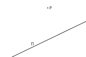
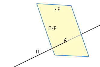
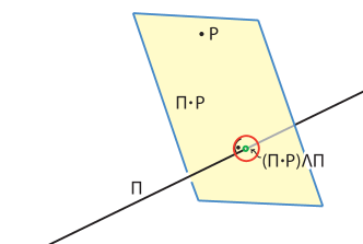
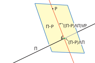
Figure 1: Geometric construction in PGA.

In PGA, geometric primitives such as points, lines, and planes, are represented by vectors of different grades, as in an exterior algebra. A plane is a 1-vector, a line is a 2-vector, and a point is a 3-vector. (A scalar is a 0-vector; we’ll meet 4-vectors in Sect. 4.4). Hence the algebra is called a graded algebra.

Each grade forms a vector space closed under addition and scalar multiplication. An element of the GA is called a multivector and is the sum of such $k$-vectors. The grade-$k$ part of a multivector $\mathbf{M}$ is written $\langle\mathbf{M}\rangle_{k}$. The geometric relationships between primitives is expressed via the geometric product that we want to experience in this example. The geometric product ${\mathbf{\Pi}}\mathbf{P}$, for example, of a line ${\mathbf{\Pi}}$ (a 2-vector) and a point $\mathbf{P}$ (a 3-vector) consists two parts, a 1-vector and a 3-vector. We write this as:

$${\mathbf{\Pi}}\mathbf{P}=\langle{\mathbf{\Pi}}\mathbf{P}\rangle_{1}+\langle{\mathbf{\Pi}}\mathbf{P}\rangle_{3}$$

1. $\langle{\mathbf{\Pi}}\mathbf{P}\rangle_{1}$ is the plane perpendicular to ${\mathbf{\Pi}}$ passing through $\mathbf{P}$. As the lowest-grade part of the product, it is written as ${\mathbf{\Pi}}\cdot\mathbf{P}$.

2. $\langle{\mathbf{\Pi}}\mathbf{P}\rangle_{3}$ is the normal direction to the plane spanned by ${\mathbf{\Pi}}$ and $\mathbf{P}$. We won’t need it for this exercise.

The sought-for line ${\mathbf{\Sigma}}$ can then be constructed as shown in Fig. 1:

1. ${\mathbf{\Pi}}\cdot\mathbf{P}$ is the plane through $\mathbf{P}$ perpendicular to ${\mathbf{\Pi}}$,

2. The point $({\mathbf{\Pi}}\cdot\mathbf{P})\wedge{\mathbf{\Pi}})$ is the meet ($\wedge$) of ${\mathbf{\Pi}}\cdot\mathbf{P}$ with ${\mathbf{\Pi}}$,

3. The line ${\mathbf{\Sigma}}:=(({\mathbf{\Pi}}\cdot\mathbf{P})\wedge{\mathbf{\Pi}})\vee\mathbf{P}$ is the join ($\vee$) of this point with $\mathbf{P}$.

The meet ($\wedge$) and joint ($\vee$) operators are part of the exterior algebra contained in the geometric algebra and are discussed in more detail below in Sect. 5.7.

The next two examples show how euclidean motions (reflections, rotations, translations) are implemented in PGA.

4.3 Example 2: A 3D Kaleidoscope

     

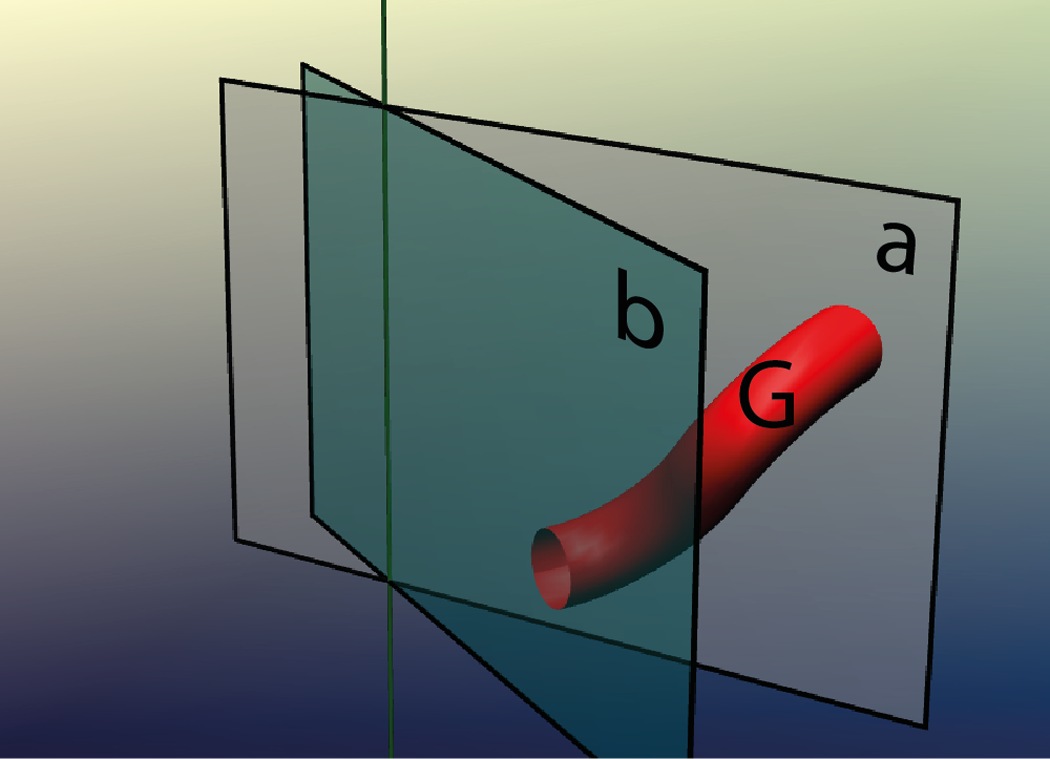
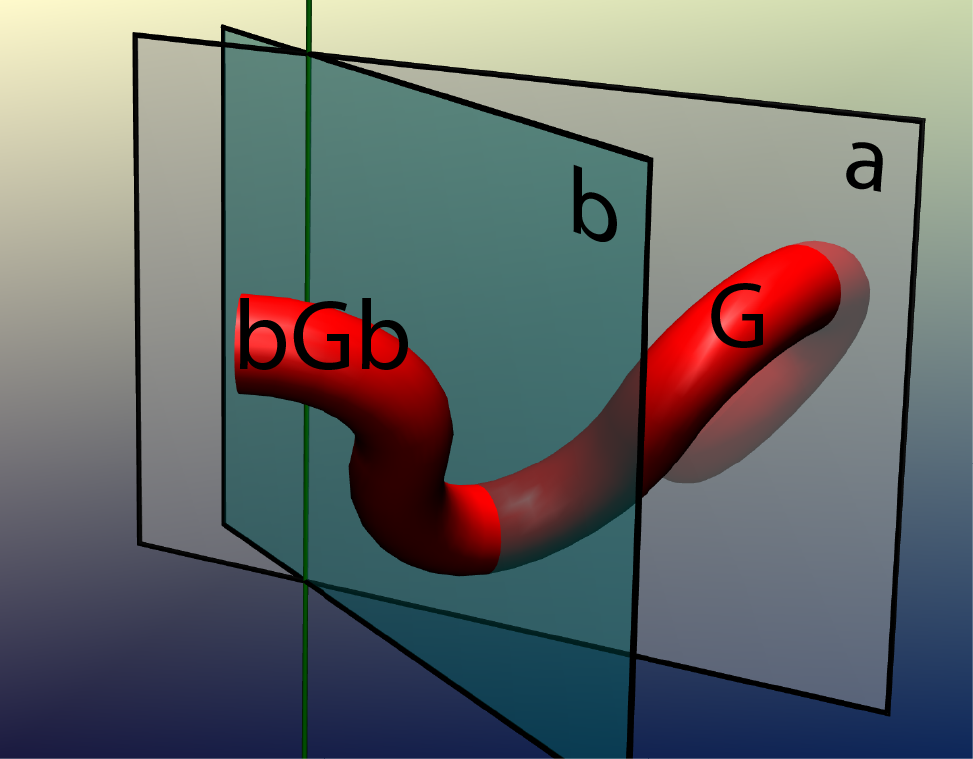
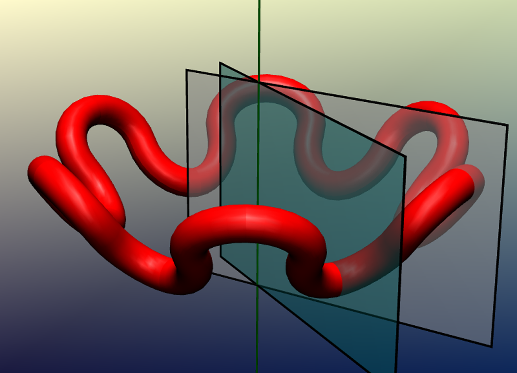
Figure 2: Creating a 3D kaleidoscope in PGA using sandwich operators.

Task: A $k$-kaleidoscope is a pair of mirror planes $\mathbf{a}$ and $\mathbf{b}$ in $\mathbf{E}^{3}$ that meet at an angle $\frac{\pi}{k}$. Given some geometry $\mathbf{G}$ generate the view of $\mathbf{G}$ seen in the kaleidoscope.

In PGA, $\mathbf{a}$ is a 1-vector. We can and do normalize this 1-vector to satisfy $\mathbf{a}^{2}=1$, where $\mathbf{a}^{2}$ is the geometric product of $\mathbf{a}$ with itself. The geometric reflection in plane $\mathbf{a}$ is implemented in PGA by the “sandwich” operator $\mathbf{a}\mathbf{G}\mathbf{a}$ (where $\mathbf{G}$ may be any $k$-vector – plane, line or point). See Fig. 2. The left-most image shows the setup, where $\mathbf{G}$ is a red tube (modeled by some combination of 1-, 2-, and 3-vectors) stretching between the two planes. The middle image shows the result of applying the sandwich $\mathbf{b}\mathbf{G}\mathbf{b}$ to the geometry (behind plane $\mathbf{a}$ one can also see $\mathbf{a}\mathbf{G}\mathbf{a}$, unlabeled). The fact that $\mathbf{a}^{2}=1$ is consistent with the fact that repeating a reflection yields the identity. The right image shows the result of applying all possible alternating products of the two reflections $\mathbf{a}$ and $\mathbf{b}$ to $\mathbf{G}$ (e. g., $\mathbf{b}\mathbf{a}\mathbf{G}\mathbf{a}\mathbf{b}$, etc.). Since the mirrors meet at the angle $\frac{\pi}{6}$, this process closes up in a ring consisting of 12 copies of $\mathbf{G}$. (To be precise, $(\mathbf{a}\mathbf{b})^{6}=(\mathbf{b}\mathbf{a})^{6}=1$).

Readers familiar with quaternions may recognize a similarity to the quaternion sandwich operators that implement 3D rotations – but here the basic sandwiches implement reflections. The next example derives sandwich operators for rotations without using reflections.

4.4 Example 3: A continuous 3D screw motion

Task: Represent a continuous screw motion in 3D.

The general orientation-preserving isometry of $\mathbf{E}^{3}$ is a screw motion, that rotates around a unique fixed line (the axis) while translating parallel to it. The ratio of the translation distance to the angle of rotation (in radians) is called the pitch of the screw motion. A rotation has pitch 0, and translation has pitch “$\infty$”.

     

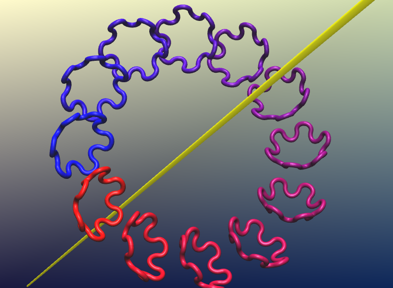
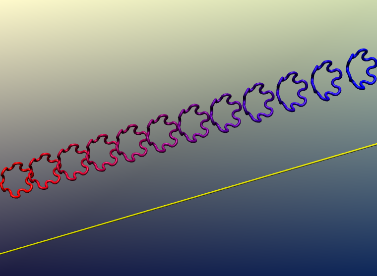
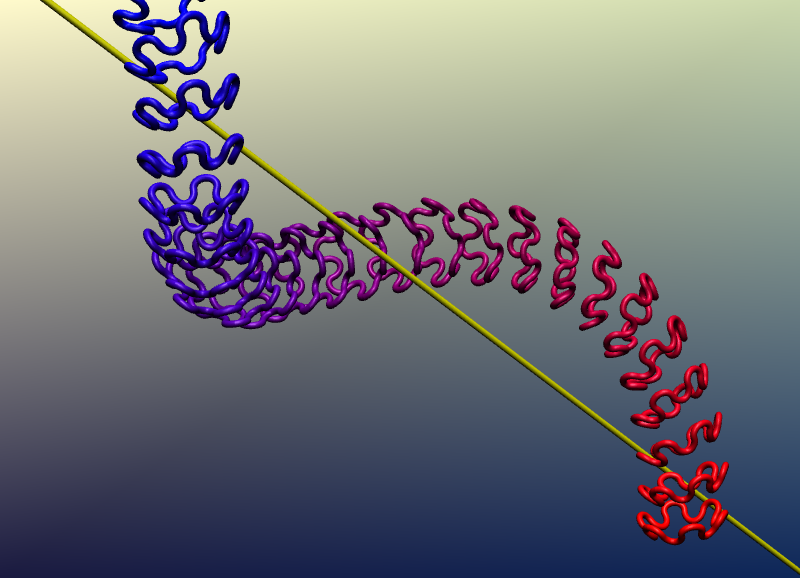
Figure 3: Continuous rotation, translation, and screw motion in PGA by exponentiating a bivector.

The previous example already contains rotations: a reflection in a plane $\mathbf{a}$ followed by a reflection in a second plane $\mathbf{b}$ (i. e., $\mathbf{b}(\mathbf{a}\mathbf{G}\mathbf{a})\mathbf{b}$) is a rotation around their common line by twice the angle between them, in this case $\frac{\pi}{3}$. Here we use a different approach to obtain a desired rotation directly from its axis of rotation. A line in $\mathbf{E}^{3}$, passing through the point $\mathbf{P}$ with direction vector $\mathbf{V}$, is given by the join operation ${\mathbf{\Omega}}:=\mathbf{P}\vee\mathbf{V}$ (yellow line in Fig. 3). We can and do normalize ${\mathbf{\Omega}}$ to satisfy ${\mathbf{\Omega}}^{2}=-1$. (Where ${\mathbf{\Omega}}^{2}$ means multiply ${\mathbf{\Omega}}$ by itself using the geometric product.) To obtain the rotation around ${\mathbf{\Omega}}$ of angle $\alpha$ define the motor $e^{t{\mathbf{\Omega}}}$. The exponential function is evaluated using the geometric product in the formal power series of $e(x)$; it behaves like the imaginary exponential $e^{ti}$ since ${\mathbf{\Omega}}^{2}=-1$. The sandwich operator $e^{t{\mathbf{\Omega}}}\mathbf{G}e^{-t{\mathbf{\Omega}}}$ implements the continuous rotation around ${\mathbf{\Omega}}$ applied to $\mathbf{G}$, parametrized by $t$. At $t=0$ it is the identity; and at $t=\frac{\alpha}{2}$ it represents the rotation of angle $\alpha$ around ${\mathbf{\Omega}}$. See the left image above, which shows the result for a sequence of $t$-values between $0$ and $\pi$. Readers familiar with the quaternion representation of rotations should recognize the similarity of these formulas. This isn’t accidental – see Sect. 11.3.4 below.

To obtain instead a translation in the direction of ${\mathbf{\Omega}}$, we used a different line, obtained by applying the polarity operator of PGA to ${\mathbf{\Omega}}$ to produce ${\mathbf{\Omega}}^{\perp}$. ${\mathbf{\Omega}}^{\perp}$ is the orthogonal complement of ${\mathbf{\Omega}}$, an ideal line, or so-called “line at infinity”. It consists of all directions perpendicular to ${\mathbf{\Omega}}$. If ${\mathbf{\Omega}}$ is thought of as a vertical axis, then ${\mathbf{\Omega}}^{\perp}$ is the horizon line. The orthogonal complement is obtained in PGA by multiplying by a special 4-vector, the unit pseudoscalar $\mathbf{I}$: ${\mathbf{\Omega}}^{\perp}:={\mathbf{\Omega}}\mathbf{I}$. A continuous translation in the direction of ${\mathbf{\Omega}}$ is then given by a sandwich with the translator $e^{t{\mathbf{\Omega}}^{\perp}}$. See the middle image above.

Let the pitch of the screw motion be $p\in\mathbf{R}$. Then the desired screw motion is given by a sandwich operator with the motor $e^{t({\mathbf{\Omega}}+p{\mathbf{\Omega}}^{\perp})}$. This motion can be factored as the product of a pure rotation and a pure translation in either order:

$$e^{t({\mathbf{\Omega}}+p{\mathbf{\Omega}}^{\perp})}=e^{t{\mathbf{\Omega}}}e^{tp{\mathbf{\Omega}}^{\perp}}=e^{tp{\mathbf{\Omega}}^{\perp}}e^{t{\mathbf{\Omega}}}$$

. See image on the right above.

We hope these examples have whetted your appetite to explore further. We now turn to a quick exposition of the history of PGA followed by a modern formulation of its mathematical foundations.

5 Mathematical foundations

5.1 Historical overview

Both the standard approach to doing euclidean geometry and the geometric algebra approach described here can be traced back to 16th century France. The analytic geometry of René Descartes (1596-1650) leads to the standard toolkit used today based on Cartesian coordinates and analytic geometry. His contemporary and friend Girard Desargues (1591-1661), an architect, confronted with the riddles of the newly-discovered perspective painting, invented projective geometry, containing additional, so-called ideal, points where parallel lines meet. Projective geometry is characterized by a deep symmetry called duality, that asserts that every statement in projective geometry has a dual partner statement, in which, for example, the roles of point and plane, and of join and intersect, are exchanged. More importantly, the truth content of a statement is preserved under duality. We will see below that duality plays an important role in PGA.

Mathematicians in the 19th century (Cayley and Klein) showed how, using an algebraic structure called a quadratic form, the euclidean metric could be built back into projective space. (The same technique also worked to model the newly discovered non-euclidean metrics of hyperbolic and elliptic geometry in projective space.) This Cayley-Klein model of metric geometry forms an essential foundation of PGA. While these developments were underway in geometry, William Hamilton and Herman Grassmann discovered surprising new algebraic structures for geometry. All these dramatic developments flowed together into William Clifford’s invention of geometric algebra in 1878 ([Cli78]). We now turn to studying from a modern perspective the ingredients of geometric algebra.

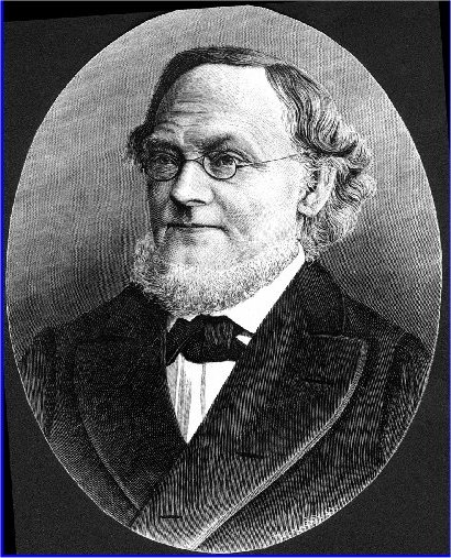
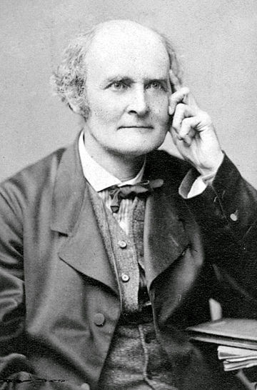
Figure 4: Important figures in the development of PGA (l. to r.): Hermann Grassmann (1809-1877), Arthur Cayley (1821-1895), Felix Klein (1849-1925), William Clifford (1845-1879).

5.2 Vector spaces

We assume that the reader is familiar with the concept of a real vector space of dimension $n$, where $n$ is the cardinality of a maximal linearly independent set of elements, called vectors. Vectors are often thought of as $n$-tuples of numbers: these arise through the choice of a basis for the vector space, and represent the coordinates of that vector with respect to the basis. A vector space is closed under addition and scalar multiplication. For each vector space $\mathbf{V}$ there exists an isomorphic dual vector space $\mathbf{V}^{*}$, consisting of dual vectors, or co-vectors. A co-vector $\mathbf{\theta}$ is a linear functional that can be evaluated at a vector $\mathbf{v}$ to produce a real number: $\langle\mathbf{\theta},\mathbf{v}\rangle\in\mathbb{R}$. This evaluation map is bilinear. It is not an inner product, that is defined on pairs of vectors. See the next section below.

Example.. When $n=3$, $\mathbf{v}$ can be interpreted as a line through the origin and $\mathbf{\theta}$, as a plane through the origin, and $\langle\mathbf{\theta},\mathbf{v}\rangle\in\mathbb{R}=0\leftrightarrow\mathbf{v}$ lies in the plane $\mathbf{\theta}$.

5.3 Normed vector spaces

A real vector space $\mathbf{V}$ of dimension $n$ has no way to measure angles or distances between elements. For that, introduce a symmetric bilinear form $B:\mathbf{V}\times\mathbf{V}\rightarrow\mathbb{R}$. $B$ is a map satisfying

1. $B(\alpha\mathbf{u}_{1}+\beta\mathbf{u}_{2},\mathbf{v})=\alpha B(\mathbf{u}_{1},\mathbf{v})+\beta B(\mathbf{u}_{2},\mathbf{v})$ (bilinearity), and

2. $B(\mathbf{u},\mathbf{v})=B(\mathbf{v},\mathbf{u})$ (symmetry).

A symmetric bilinear form $B$ can be rewritten as an inner product on vectors: $\mathbf{u}\cdot\mathbf{v}:=B(\mathbf{u},\mathbf{v})$ and used to define a norm, or length-function, on vectors: $\|\mathbf{u}\|:=\sqrt{|{\mathbf{u}\cdot\mathbf{u}}|}$. $\mathbb{R}^{n}$ is a normed vector space. The next section classifies symmetric bilinear forms.

5.4 Sylvester signature theorem

Symmetric bilinear forms of dimension $n$ can be completely characterized by three positive integers $(p,m,z)$ satisfying $p+m+z=n$. Sylvester’s Theorem asserts that for any such $B$ there is a unique choice of $(p,m,z)$ and a basis $\{\mathbf{e}_{i}\}$ for $\mathbf{V}$ such that

1. $\mathbf{e}_{i}\cdot\mathbf{e}_{j}=0$ for $i\neq j$ (orthogonal basis), and

2. $$\mathbf{e}_{i}\cdot\mathbf{e}_{i}=\begin{cases}1&\leavevmode\nobreak\ \text{for}\leavevmode\nobreak\ 1\leq i\leq p\\ -1&\leavevmode\nobreak\ \text{for}\leavevmode\nobreak\ p<i\leq p+m\leavevmode\nobreak\ \leavevmode\nobreak\ \leavevmode\nobreak\ \leavevmode\nobreak\ \leavevmode\nobreak\ \leavevmode\nobreak\ \leavevmode\nobreak\ \text{(normalized basis)}\\ 0&\leavevmode\nobreak\ \text{for}\leavevmode\nobreak\ p+m<i\leq n\end{cases}$$

Example. Taking $n=3$ and $(p,m,z)=(3,0,0)$ we arrive at the familiar euclidean vector space $\mathbb{R}^{3}$ with norm $\|(x,y,z)\|=\sqrt{x^{2}+y^{2}+z^{2}}$ where $(x,y,z)$ are coordinates in an orthonormal basis.

5.5 Euclidean space $\mathbf{E}^{n}$

We can transform the vector space $\mathbb{R}^{n}$ into the metric space $\mathbf{E}^{n}$ by identifying each vector of the former (also the zero vector $O$) with a point of the latter. Then define a distance function on the resulting points with $d(\mathbf{P},\mathbf{Q}):=\|\mathbf{P}-\mathbf{Q}\|$. This distance function produces a differentiable manifold $\mathbf{E}^{n}$ whose tangent space at every point is $\mathbb{R}^{n}$.

Terminology alert. When we say doing euclidean geometry we are referring to the geometry of euclidean space $\mathbf{E}^{n}$, not the euclidean vector space $\mathbb{R}^{n}$. The elements of $\mathbf{E}^{n}$ are points, those of $\mathbb{R}^{n}$ are vectors; the motions of $\mathbf{E}^{n}$ include translations and rotations, those of $\mathbb{R}^{n}$ are rotations preserving the origin $O$. $\mathbf{E}^{n}$ is intrinsically more complex than $\mathbb{R}^{n}$: the tangent space at each point is $\mathbb{R}^{n}$. See [Gun17b], §4, for a deeper analysis of this issue. We will see that euclidean PGA includes both $\mathbf{E}^{n}$ and $\mathbb{R}^{n}$ in an organic whole.

5.6 The tensor algebra of a vector space

Vector spaces have linear subspaces. The subspace structure is mirrored in the algebraic structure of the exterior algebra defined over the vector space. To define the exterior algebra cleanly, we need first to introduce the tensor algebra $T(\mathbf{V})$ over $\mathbf{V}$. This algebra is generated by multiplying arbitrary sequences of vectors together to generate a graded algebra. This product is called the tensor product and is written $\otimes$. It is bilinear. The tensor product of $k$ vectors is called a $k$-vector. The $k$-vectors form a vector space $T^{k}$. $T^{0}$ is the underlying field $\mathbb{R}$. $T(\mathbf{V})$ can be written as the direct sum of these vector spaces:

$$T=\bigoplus_{i=0}^{\infty}T^{k}$$

Obviously this is a very big and somewhat unwieldy structure, but necessary for a clean definition of important algebras below.

Example $n=2$. The tensor algebra of a 2-dimensional vector space with basis $\{\mathbf{u},\mathbf{v}\}$ has the basis:

• $T^{0}$: $\{\mathbf{1}\}$

• $T^{1}$: $\{\mathbf{u},\mathbf{v}\}$

• $T^{2}$:$\{\mathbf{u}\otimes\mathbf{u},\mathbf{u}\otimes\mathbf{v},\mathbf{v}\otimes\mathbf{u},\mathbf{v}\otimes\mathbf{v}\}$

• $T^{3}$:$\{\mathbf{u}\otimes\mathbf{u}\otimes\mathbf{u},\mathbf{u}\otimes\mathbf{u}\otimes\mathbf{v},\mathbf{u}\otimes\mathbf{v}\otimes\mathbf{u},\mathbf{u}\otimes\mathbf{v}\otimes\mathbf{v},\mathbf{v}\otimes\mathbf{u}\otimes\mathbf{u},\mathbf{v}\otimes\mathbf{u}\otimes\mathbf{v},\mathbf{v}\otimes\mathbf{v}\otimes\mathbf{u},\mathbf{v}\otimes\mathbf{v}\otimes\mathbf{v}\}$

• etc.

5.7 Exterior algebra of a vector space

The exterior algebra is obtained from the tensor algebra by declaring elements of the form $\mathbf{v}\otimes\mathbf{v}$ (where $\mathbf{u}$ and $\mathbf{v}$ are 1-vectors), to be equivalent to 0, that is, squares of 1-vectors vanish. By bilinearity, this implies

$$(\mathbf{u+v})\otimes(\mathbf{u+v})=\mathbf{u}\otimes\mathbf{u}+\mathbf{v}\otimes\mathbf{v}+\mathbf{u}\otimes\mathbf{v}+\mathbf{v}\otimes\mathbf{u}\cong 0$$

implying $\mathbf{u}\otimes\mathbf{v}\cong-\mathbf{v}\otimes\mathbf{u}$ since $\mathbf{u}\otimes\mathbf{u}\cong 0$ and $\mathbf{v}\otimes\mathbf{v}\cong 0$. Thus the quotient product is anti-symmetric on 1-vectors. The resulting quotient algebra is called the exterior algebra and its product is the exterior or wedge product, written as $\mathbf{X}\wedge\mathbf{Y}$. The product is associative, anti-symmetric on 1-vectors and distributes over addition. In general, the wedge of a $k$-vector $\mathbf{X}$ and an $m$-vector $\mathbf{Y}$ will vanish $\iff\mathbf{X}$ and $\mathbf{Y}$ are linearly-dependent subspaces, otherwise it is the $(k+m)$-vector representing the subspace span of $\mathbf{X}$ and $\mathbf{Y}$.

The exterior algebra $G(\mathbf{V})$ mirrors the subspace structure of $\mathbf{V}$. Two $k$-vectors $\mathbf{v}$ and $\alpha\mathbf{v}$ that are non-zero multiples of each other represent the same subspace but have different weights, or intensities. $G(\mathbf{V})$ is finite-dimensional since any $m$-vector in the tensor algebra with $m>n$ vanishes in the exterior algebra since any product of $n+1$ basis 1-vectors will have a repeated factor, and this is equivalent to 0. It can be written as a direct sum of its non-vanishing grades:

$$G(\mathbf{V})=\bigoplus_{i=0}^{n}{{\bigwedge}^{i}}$$

The dimension of each grade is given by $dim\left(\bigwedge^{k}\right)=\binom{n}{k}$, so the total dimension of the algebra is $\Sigma_{i=0}^{n}\binom{n}{k}=2^{n}$.

Example $n=2$. The exterior algebra of a 2-dimensional vector space with basis $\{\mathbf{u},\mathbf{v}\}$ is a 4-dimensional graded algebra:

• $\bigwedge^{0}$: $\{\mathbf{1}\}$

• $\bigwedge^{1}$: $\{\mathbf{u},\mathbf{v}\}$

• $\bigwedge^{2}$: $\{\mathbf{u}\wedge\mathbf{v}\}$

Exterior algebras were, like so many other results in this field, discovered by Hermann Grassmann ([Gra44]) and are sometimes called Grassmann algebras.

5.8 The dual exterior algebra

Important for PGA: the dual vector space $\mathbf{V}^{*}$ generates its own exterior algebra $G(\mathbf{V^{*}})=G^{*}(\mathbf{V})$. The standard exterior algebra represents the subspace structure based on subspace join, where the 1-vectors are vectors (or lines through the origin). The dual exterior algebra represents the subspace structure “turned on its head”: the 1-vectors represent hyperplanes through the origin and the wedge operation is subspace meet. The principle of duality ensures that these two approaches are completely equivalent and neither a priori is to be preferred. Each construction produces a separate exterior algebra. The dual exterior algebra is important for PGA.

The next step on our way to PGA is projective geometry.

5.9 Projective space of a vector space

An $n$-dimensional real vector space $\mathbf{V}$ can be projectivized to produce $(n-1)$ dimensional real projective space $\mathbb{R}{P^{n-1}}$. This is a quotient space constuction as in the case of the exterior algebra. Here the equivalence relation on vectors of $\mathbf{V}$ is

$$\mathbf{u}\cong\mathbf{v}\leftrightarrow\exists\lambda\neq 0\in\mathbb{R}\leavevmode\nobreak\ \leavevmode\nobreak\ \text{such that}\leavevmode\nobreak\ \leavevmode\nobreak\ \mathbf{u}=\lambda\mathbf{v}$$

One sometimes says, the points of $\mathbb{R}{P^{n}}$ are the lines through the origin of $\mathbf{V}$.

Example. $\mathbb{R}{P^{2}}$ is called the projective plane. We consider it as arising from projectivizing $\mathbb{R}^{3}$ (although the norm on $\mathbb{R}^{3}$ plays no role in the construction). Take $\mathbb{R}^{3}$ with standard basis $\{\mathbf{e}_{0},\mathbf{e}_{1},\mathbf{e}_{2}$ vectors pointing in the $x$-, $y$-, and $z$-directions, resp.) Each point $\mathbf{P}$ of the $z=1$ plane represents the line through the origin obtained by joining $\mathbf{P}$ to the origin. Hence $\mathbf{P}$ corresponds to a point of $\mathbb{R}{P^{2}}$. The only points of $\mathbb{R}{P^{2}}$ not accounted for in this way arise from lines through the origin lying in the $z=0$ plane, since such lines don’t intersect the $z=1$ plane. However in projective geometry they correspond to points; it is useful to speak of ideal points of $\mathbb{R}{P^{2}}$ where these lines intersect the plane $z=1$. The intersection of parallel planes yields in the same way an ideal line. The interplay of euclidean and ideal elements in PGA is essential to its effectiveness.

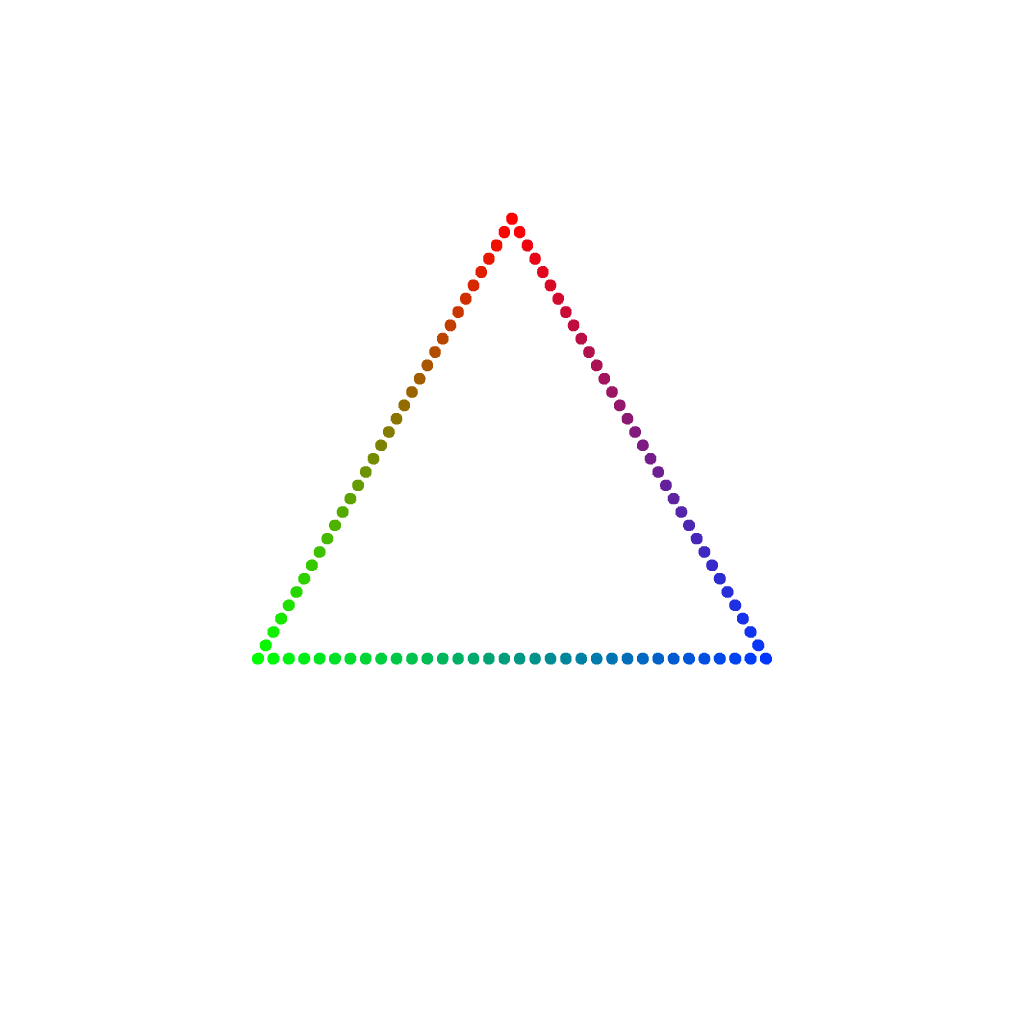
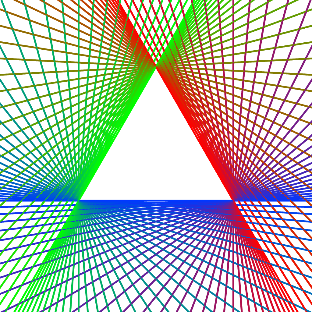
Figure 5: Traversing the boundary of a triangle (left) and a trilateral (right).

Example of duality in $\mathbb{R}{P^{2}}$. Because duality plays an essential role in PGA, we include an example here to show how it works. Following the pattern established in the $19^{th}$ century literature we use a two-column format to present, on the left, a geometric configuration in the projective plane and, on the right, its dual configuration. Dualized terms have been highlighted in color. Fig. 5 illustrates this example.

A triangle is determined by three points, called its vertices. The pair-wise joining lines of the vertices are the sides of the triangle. To traverse the boundary of the triangle, move a point from one vertex to the next vertex along their common side, then take a turn and continue moving along the next side. Continue until arriving back at the original vertex.

A trilateral is determined by three lines, called its sides. The pair-wise intersection points of the sides are the vertices of the trilateral. To traverse the boundary of the trilateral, rotate a line from one side to the next around their common vertex, then shift over and continue rotating round the next vertex. Continue until arriving back at the original side.

Perhaps you can experience that the left-hand example is somehow more familiar than the right-hand side. After all, we learn about triangles in school, not trilaterals. This seems to be related to the fact that we think of points as being the basic elements of geometry (and reality) out of which other elements (lines, planes) are built. We’ll see below in Sect. 6.4 however that PGA in important respects challenges us to think in the right-hand mode.

Why projectivize? Working in projective space guarantees that the meet of parallel lines and planes, as well as the join of euclidean and ideal elements, are handled seamlessly, without “special casing” – one of the features on our initial wish-list. Furthermore we’ll see that only in projective space can we represent translations.

5.10 Projective exterior algebras

The same construction applied to create $\mathbb{R}{P^{n}}$ from $\mathbf{V}$ can be applied to the Grassmann algebras $G(\mathbf{V})$ and $G^{*}(\mathbf{V})$ to obtain projective exterior algebras. We denote these projectivized versions as $\mathbf{P}(G(\mathbf{V}))$ and $\mathbf{P}(G^{*}(\mathbf{V})$. Here we use an $(n+1)$-dimensional $\mathbf{V}$ so that we obtain $\mathbb{R}{P^{n}}$ by projectivizing. The resulting exterior algebras mirror the subspace structure of $\mathbb{R}{P^{n}}$: 1-vectors in $G$ represent points in $\mathbf{P}(G)$, 2-vectors represent lines, etc., and $\wedge$ is projective join. In the dual algebra $G^{*}$, 1-vectors are hyperplanes ($(n-1)$-dimensional subspaces), and $n$-vectors represent points, while $\wedge$ is the meet operator. More generally: in a standard projective exterior algebra $\mathbf{P}(G)$, the elements of grade $k$ for $k=1,2,...n$, represent the subspaces of dimension $k-1$. For example, for $n=2$, the 1-vectors are points, and the 2-vectors are lines. The graded algebra also has elements of grade 0, the scalars (the real numbers $\mathbb{R}$); and elements of grade $(n+1)$ (the highest non-zero grade), the pseudoscalars.

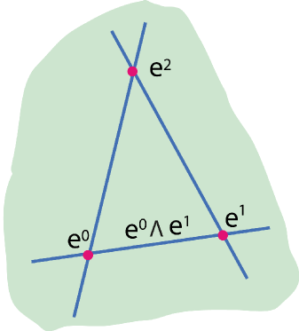
Figure 6: Left: The plane $\mathbf{e}^{0}\wedge\mathbf{e}^{1}\wedge\mathbf{e}^{2}$ (green) created by joining 3 points in $\mathbf{P}(G)$, the standard exterior algebra (written with raised indices). Right: The meeting point $\mathbf{e}_{0}\wedge\mathbf{e}_{1}\wedge\mathbf{e}_{2}$ (green) of three planes in $\mathbf{P}(G^{*})$, the dual exterior algebra (written with lowered indices).

Example.Fig. 6 shows how the wedge product of three points in $\mathbf{P}(G)$ is a plane, while the wedge product of three planes in $\mathbf{P}(G^{*})$ is a point. Notice the use of subscripts and superscripts to distinguish between the two algebras.

5.10.1 Dimensions of projective subspaces

It’s important for what follows to clarify the notion of the dimension of a subspace. We are accustomed to say that a point in $\mathbb{R}{P^{n}}$ is a 0-dimensional subspace. This is indeed the case in the context of the standard exterior algebra where points are represented by 1-vectors. Then all other linear subspaces are built up out of the 1-vectors by wedging (joining) points together. The dimension counts how many 1-vectors are needed to generate a subspace. For example, a line (2-vector) can be represented as the join of two points $\ell=\mathbf{A}\wedge\mathbf{B}$. $\ell$ is 1-dimensional since there is a one-parameter set of points incident with the line, given by $\alpha\mathbf{A}+\beta\mathbf{B}$ where only the ratio $\alpha:\beta$ matters. A line considered as a set of incident points is called a point range. In general, if you wedge together $k$ linearly independent points you obtain a $k-1$-dimensional subspace. For let $\mathbf{X}=\mathbf{P}_{1}\wedge...\wedge\mathbf{P}_{k}$. Then $\mathbf{X}\wedge\mathbf{P}=0\iff\mathbf{P}\cong\alpha_{1}\mathbf{P}_{1}+...+\alpha_{k}\mathbf{P}_{k}$ for real constants $\{\alpha_{i}\}$. Since we are working in projective space, this is a $(k-1)$-dimensional set of points ($\{\alpha_{i}\}\equiv\beta\{\alpha_{i}\}$ for non-zero $\beta$).

When we apply this reasoning to the dual exterior algebra, we are led to the surprising conlusion that a plane (a 1-vector) is 0-dimensional, since all the other linear subspaces are built up from planes by the meet operation. That is, in the dual algebra planes are simple and indivisible, just as a point in the standard algebra is. A line (2-vector) is the meet of two planes $\ell=\mathbf{a}\wedge\mathbf{b}$. $\ell$ is 1-dimensional since there is a one-parameter set of planes incident with the line, given by $\alpha\mathbf{a}+\beta\mathbf{b}$ where only the ratio $\alpha:\beta$ matters. A line considered as a set of incident planes is called a plane pencil. It’s the form you get if you spin a plane around one of its lines. The meet of three planes is a point. The set of all planes incident with the point is 2-dimensional, called a plane bundle, etc. To think in this way you have to overcome certain habits that associate dimension with extensive “size”.

Take-away. The dimension of a geometric primitive depends on whether it is viewed in the standard exterior algebra or the dual exterior algebra. The 1-vectors serve as the “building block” in both cases. For example, in the standard algebra a point is 0-dimensional, simple, and indivisible. In the dual algebra, however, it is two-dimensional, since it is created by wedging together three planes, or, what is the same, there is a two-parameter family of planes incident with it.

5.10.2 Poincaré duality

Every geometric entity $x$ (e.g., point, line, plane) occurs once in each exterior algebra, say as $\mathbf{x}\in\mathbf{P}(G)$ and as $\mathbf{x}^{*}\in\mathbf{P}(G^{*})$. The Poincaré duality map $J:\mathbf{P}(G)\rightarrow\mathbf{P}(G^{*})$ is defined by $\mathbf{x}\rightarrow\mathbf{x}^{*}$. It is essentially an identity map, sometimes called the “dual coordinates” map. In particular it is invertible. When often use $J$ for both maps when there is no danger of confusion. $J$ is a grade-reversing map, that is a vector space isomorphism $\bigwedge^{k}\leftrightarrow\bigwedge^{n+1-k}$ for all $k$. See [Gun11a] §2.3.1 for details.

5.10.3 The regressive product

Using $J$, it’s possible to “import” the outer product from one algebra into the the other. This imported product is sometimes called the regressive product to distinguish it from the native wedge product. For example, it possible to define a join operator $\vee$ in $\mathbf{P}(G^{*})$ by

$$\mathbf{X}\vee\mathbf{Y}:=J^{-1}(J(\mathbf{X})\wedge J(\mathbf{Y}))$$

where the $\wedge$ on the right-hand side is that of the algebra $\mathbf{P}(G)$. In this way, join and meet are available within a single algebra. We’ll see below in Sect. 6.4 why this is important for PGA . We write the outer product of $\mathbf{P}(G^{*})$, the meet operator, as $\wedge$, and the join operator, imported from $\mathbf{P}(G)$, as $\vee$. That’s easy to remember due to their similarity to the set operations $\cap$ and $\cup$.

References. The above mathematical prerequisites can be well-studied on Wikipedia in the articles on: vector space, bilinear form, quadratic form, tensor algebra, exterior algebra, and projective space. We turn now to the geometric product and associated geometric product.

6 Geometric product and geometric algebra

The exterior algebra of $\mathbb{R}{P^{n}}$ answers questions regarding incidence (meet and join) of projective subspaces. That’s an important step and yields uniform representation of points, lines, and planes as well as a “parallel-safe” meet and join operators, both features from our wish-list.

However the exterior algebra knows nothing about measurement, such as angle and distance, crucial to euclidean geometry. To overcome this we refine the equivalence relation that we used to produce the exterior algebra from the tensor algebra T. Instead of requiring that $\mathbf{v}\otimes\mathbf{v}\cong 0$ we require that

$$\mathbf{v}\otimes\mathbf{v}-B(\mathbf{v},\mathbf{v})\cong 0$$

where $B$ is a symmetric bilinear form, that is $\mathbf{v}\otimes\mathbf{v}$ is equivalent to a scalar but not necessarily to 0 as in an exterior algebra. We define the geometric algebra with inner product $B$ to be the quotient of the tensor algebra by this new equivalence relation. Since this relation encodes an inner product on vectors, the geometric product contains more information than the exterior product. We write the geometric product using simple juxtaposition: $\mathbf{X}\mathbf{Y}$.

Since the square of every 1-vector reduces to a scalar (0-vector), we obtain the same finite-dimensional graded algebra structure for the geometric algebra as for the exterior algebra, described in Sect. 5.7. In fact, as we now show, one can also construct the geometric algebra by extending the exterior algebra.

Alternative formulation.. Define the geometric product of two 1-vectors $\mathbf{u}$ and $\mathbf{v}$ to be

$$\mathbf{u}\mathbf{v}:=\mathbf{u}\cdot\mathbf{v}+\mathbf{u}\wedge\mathbf{v}$$

where $\cdot$ is the inner product associated to $B$ and $\wedge$ is the wedge product in the associated exterior algebra. (I. e., skip the tensor algebra formulation entirely.) Then it’s possible to show that this geometric product has a unique extension to the whole graded algebra that agrees with the geometric product obtained above using the more abstract tensor product construction.

Connection to exterior algebra. The geometric algebra reduces to the exterior algebra when $B$ is trivial: $B(\mathbf{u},\mathbf{v})=0$, equivalent to a signature of $(0,0,n)$.

6.1 Projective geometric algebra

In order to apply the Cayley-Klein construction for modeling metric spaces such as euclidean space, we work in projective space. That is, we interpret the geometric product in a projective setting just as we did with the wedge product in the projectivized exterior algebra. We call the result a projective geometric algebra or PGA for short. It uses $(n+1)$-dimensional coordinates to model $n-$ dimensional euclidean geometry. The standard geometric algebra based on $\mathbf{P}(G)$ with signature $(p,m,z)$ is denoted $\mathbf{P}(\mathbb{R}_{p,m,z})$. The dual version of the same (based on $\mathbf{P}(G^{*})$) is written $\mathbf{P}(\mathbb{R}^{*}_{p,m,z})$.

Remark. PGA is actually a whole family of geometric algebras, one for each signature; the rest of these notes concern finding and exploring the member of this family that models euclidean geometry. We often write “PGA” for this one algebra – we sometimes use the more precise “EPGA” for ”euclidean” PGA to avoid confusion.

6.2 Geometric algebra basics

In general, the geometric product of a $k$-vector and an $m$-vector is a sum of components of different grades, each expressing a different geometric aspect of the product, as in the geometric product of two 1-vectors above. A general element containing different grades is called a multivector. A multivector $\mathbf{M}$ can be written then as a sum of different grades: $\mathbf{M}=\sum_{i=0}^{n}\langle\mathbf{M}\rangle_{i}$. For example, we can write the above geometric product of two 1-vectors as: $\mathbf{a}\mathbf{b}:=\langle\mathbf{a}\mathbf{b}\rangle_{0}+\langle\mathbf{a}\mathbf{b}\rangle_{2}$. The product of two multivectors can be reduced to a sum of products of single-grade vectors, so we concentrate our discussions on the latter.

The highest grade part of the product is the $(k+m)$-grade part, and coincides with the $\wedge$ product in the exterior algebra. All the other parts of the product involve some “contraction” due to the square of a 1-vector reducing to a scalar (0-vector), which drops the dimension of the product down by two for each such square. We define the lowest-grade part of the geometric product of a $k$-vector and an $m$-vector to be the inner product and write $\mathbf{a}\cdot\mathbf{b}$ (it does not have to be a scalar!). It has grade $|k-m|$.

We will occasionally also need the commutator product $\mathbf{X}\times\mathbf{Y}:=\frac{1}{2}(\mathbf{X}\mathbf{Y}-\mathbf{Y}\mathbf{X})$, the so-called anti-symmetric part of the geometric product. A $k$-vector which can be written as the product of 1-vectors is called a simple $k$-vector. Note that then all the 1-vectors are orthogonal to each other and the product is equal to the wedge product of the 1-vectors. Any multi-vector can be written as a sum of simple $k$-vectors. We sometimes call 2-vectors bivectors, and 3-vectors, trivectors.

We’ll also need the reverse operator $\widetilde{\mathbf{X}}$, that reverses the order of the products of 1-vectors in a simple $k$-vector. If the simple $k$-vector is $\mathbf{X}$, then the reverse $\widetilde{\mathbf{X}}=(-1)^{k\choose 2}\mathbf{X}$. The exponent counts how many “neighbor flips” are required to reverse a string with $k$ characters (since for orthogonal 1-vectors $\mathbf{a}$ and $\mathbf{b}$, $\mathbf{b}\mathbf{a}=-\mathbf{a}\mathbf{b}$).

We first explore the algebra $\mathbf{P}(\mathbb{R}_{3,0,0})$ in order to warm up in a familiar setting.

6.3 Example: Spherical geometry via $\mathbf{P}(\mathbb{R}_{3,0,0})$

This is the projectivized geometric algebra of $\mathbb{R}^{3}$, the familiar 3D euclidean vector space. Take an orthonormal basis $\{\mathbf{e}_{0},\mathbf{e}_{1},\mathbf{e}_{2})$. Then a general 1-vector is given by $\mathbf{u}=x\mathbf{e}_{0}+y\mathbf{e}_{1}+z\mathbf{e}_{2}$. It satisfies $\mathbf{u}^{2}=x^{2}+y^{2}+z^{2}=\|\mathbf{u}\|^{2}$. The set of 1-vectors satisfying $\|\mathbf{u}\|=1$ forms the unit sphere (whereby $\mathbf{u}$ and $-\mathbf{u}$ represent the same projective point in the algebra). We saw above, the product of two normalized 1-vectors is given by $\mathbf{u}\mathbf{v}:=\mathbf{u}\cdot\mathbf{v}+\mathbf{u}\wedge\mathbf{v}$. Here $\mathbf{u}\cdot\mathbf{v}=\cos{\alpha}$ where $\alpha$ is the angle between the spherical points $\mathbf{u}$ and $\mathbf{v}$, and $\mathbf{u}\wedge\mathbf{v}$ is the line (2-vector) spanned by the points (represented by a great circle joining the points.)

An orthonormal basis for the 2-vectors is given by

$$\{\mathbf{E}_{0}:=\mathbf{e}_{1}\mathbf{e}_{2},\leavevmode\nobreak\ \mathbf{E}_{1}:=\mathbf{e}_{2}\mathbf{e}_{0},\leavevmode\nobreak\ \mathbf{E}_{2}:=\mathbf{e}_{0}\mathbf{e}_{1}\}$$

These are three mutually perpendicular great circles. The unit pseudo-scalar is $\mathbf{I}:=\mathbf{e}_{012}:=\mathbf{e}_{0}\mathbf{e}_{1}\mathbf{e}_{2}$. Multiplication of either a $1$- or $2$-vector with $\mathbf{I}$ produces the orthogonal complement $\mathbf{X}^{\perp}$ of the argument $\mathbf{X}$. That is, $\mathbf{u}^{\perp}=\mathbf{u}\mathbf{I}$ is the great circle that forms the “equator” to the “pole” point represented by $\mathbf{u}$; $\mathbf{U}\mathbf{I}$ for a 2-vector $\mathbf{U}$ produces the polar point of the “equator” represented by $\mathbf{U}$. The complete $8x8$ multiplication table is shown in Table 1.

Exercise.. Check in the multiplication table that the products $\mathbf{e}_{i}\mathbf{I}=\mathbf{E}_{i}$ and $\mathbf{E}_{i}\mathbf{I}=-\mathbf{e}_{i}$ for $i\in\{1,2,3\}$ and verify that these results confirm that multiplication by $\mathbf{I}$ is the “orthogonal complement” operator.

	$\mathbf{1}$	$\mathbf{e}_{0}$	$\mathbf{e}_{1}$	$\mathbf{e}_{2}$	$\mathbf{E}_{0}$	$\mathbf{E}_{1}$	$\mathbf{E}_{2}$	$\mathbf{I}$
$\mathbf{1}$	$\mathbf{1}$	$\mathbf{e}_{0}$	$\mathbf{e}_{1}$	$\mathbf{e}_{2}$	$\mathbf{E}_{0}$	$\mathbf{E}_{1}$	$\mathbf{E}_{2}$	$\mathbf{I}$
$\mathbf{e}_{0}$	$\mathbf{e}_{0}$	$1$	$\mathbf{E}_{2}$	$-\mathbf{E}_{1}$	$\mathbf{I}$	$-\mathbf{e}_{2}$	$\mathbf{e}_{1}$	$\mathbf{E}_{0}$
$\mathbf{e}_{1}$	$\mathbf{e}_{1}$	$-\mathbf{E}_{2}$	$\mathbf{1}$	$\mathbf{E}_{0}$	$\mathbf{e}_{2}$	$\mathbf{I}$	$-\mathbf{e}_{0}$	$\mathbf{E}_{1}$
$\mathbf{e}_{2}$	$\mathbf{e}_{2}$	$\mathbf{E}_{1}$	$-\mathbf{E}_{0}$	$\mathbf{1}$	$-\mathbf{e}_{1}$	$\mathbf{e}_{0}$	$\mathbf{I}$	$\mathbf{E}_{2}$
$\mathbf{E}_{0}$	$\mathbf{E}_{0}$	$\mathbf{I}$	$-\mathbf{e}_{2}$	$\mathbf{e}_{1}$	$-\mathbf{1}$	$-\mathbf{E}_{2}$	$\mathbf{E}_{1}$	$-\mathbf{e}_{0}$
$\mathbf{E}_{1}$	$\mathbf{E}_{1}$	$\mathbf{e}_{2}$	$\mathbf{I}$	$-\mathbf{e}_{0}$	$\mathbf{E}_{2}$	$-\mathbf{1}$	$-\mathbf{E}_{0}$	$-\mathbf{e}_{1}$
$\mathbf{E}_{2}$	$\mathbf{E}_{2}$	$-\mathbf{e}_{1}$	$\mathbf{e}_{0}$	$\mathbf{I}$	$-\mathbf{E}_{1}$	$\mathbf{E}_{0}$	$-\mathbf{1}$	$-\mathbf{e}_{2}$
$\mathbf{I}$	$\mathbf{I}$	$\mathbf{E}_{0}$	$\mathbf{E}_{1}$	$\mathbf{E}_{2}$	$-\mathbf{e}_{0}$	$-\mathbf{e}_{1}$	$-\mathbf{e}_{2}$	$-\mathbf{1}$

Table 1: Multiplication table for $\mathbf{P}(\mathbb{R}_{3,0,0})$, the geometric algebra of the sphere.

Exercise. Show that the angle $\alpha$ between two normalized 2-vectors (great circles) in $\mathbf{P}(\mathbb{R}_{3,0,0})$ is given by $\alpha=\cos^{-1}{(\mathbf{U}\cdot\mathbf{V})}$.

Exercise. Verify that the elements $\{1,\mathbf{e}_{12},\mathbf{e}_{20},\mathbf{e}_{01}\}$ generates a sub-algebra of $\mathbf{P}(\mathbb{R}_{3,0,0})$ that is isomorphic to Hamilton’s quaternion algebra $\mathbb{H}$ generated by $\{1,i,j,k\}$.

Exercise. Find as many formulas of spherical geometry/trigonometry as you can within $\mathbf{P}(\mathbb{R}_{3,0,0})$.

Exercise. $\mathbf{P}(\mathbb{R}^{*}_{3,0,0})$ is the same algebra as above but uses the dual construction where the 1-vectors are lines (great circles). Show that it also provides a model for spherical geometry, one in which the $\mathbf{U}\cdot\mathbf{V}=\cos{\alpha}$ for normalized 1-vectors $\mathbf{U}$ and $\mathbf{V}$ meeting at angle $\alpha$.

The above discussion gives a rudimentary demonstration of how the signature $(3,0,0)$ leads to a model of spherical geometry in both the standard and dual constructions

We now turn to the question of which member of the PGA family models the euclidean plane. That is, we need to determine a signature and, possibly, choose between the standard and dual construction. The existence of parallel lines in euclidean geometry plays an essential role in this search.

6.4 Determining the signature for euclidean geometry

We saw that the inner product of 1-vectors in $\mathbf{P}(\mathbb{R}^{*}_{3,0,0})$ can be used to compute the angle between two lines in spherical geometry. What does the analogous question in the euclidean plane yield? Let

$$a_{0}x+b_{0}y+c_{0}=0,\leavevmode\nobreak\ \leavevmode\nobreak\ \leavevmode\nobreak\ \leavevmode\nobreak\ \leavevmode\nobreak\ \leavevmode\nobreak\ \leavevmode\nobreak\ a_{1}x+b_{1}y+c_{1}=0$$

be two oriented lines which intersect at an angle $\alpha$. We can assume without loss of generality that the coefficients satisfy ${a_{i}^{2}+b_{i}^{2}=1}$. Then it is not difficult to show that $a_{0}a_{1}+b_{0}b_{1}=\cos{\alpha}$. One can observe for example that the direction of line $i$ is $(-b_{i},a_{i})$ and calculate the angle of these direction vectors.

Figure 7: Angles of euclidean lines.

The superfluous coordinate. The third coordinate of the lines makes no difference in the angle calculation! Indeed, translating a line changes only its third coordinate, leaving the angle between the lines unchanged. Refer to Fig. 7 which shows an example involving a general line and a pair of horizontal lines. Choose a basis for the (dual) projective plane so that $\mathbf{e}_{1}$ corresponds to the line $x=0$, $\mathbf{e}_{2}$ to $y=0$, and $\mathbf{e}_{0}$ to $z=0$. Then the line given by $ax+by+c=0$ corresponds to the 1-vector $c\mathbf{e}_{0}+a\mathbf{e}_{1}+b\mathbf{e}_{2}$. If the geometric product of two such 1-vectors is to produce $a_{1}a_{2}+b_{1}b_{2}$ then the signature has to be $(2,0,1)$. Hence the proper PGA for $\mathbf{E}^{2}$ is $\mathbf{P}(\mathbb{R}^{*}_{2,0,1})$. Such a signature, or metric, is called degenerate since $z\neq 0$.

Reminder: The $*$ in the name says that the algebra is built on $\mathbf{P}(G^{*})$, the dual exterior algebra, since the inner product is defined on lines instead of points. A similar argument applies in dimension $n$, yielding the signature $(n,0,1)$ for $\mathbf{E}^{n}$. $\mathbf{P}(\mathbb{R}_{n,0,1})$ models a qualitatively different metric space called dual euclidean space.

Degenerate metric: asset or liability? PGA’s development reflects the fact that much of the existing literature on geometric algebras deals only with non-degenerate metrics, reflecting widespread prejudices regarding degenerate metrics. (See [Gun17b] for a thorough analysis and refutation of these misconceptions.) After long experience we are convinced that the degenerate metric, far from being a liability, is an important part of PGA’s success – exactly the degenerate metric models the metric relationships of euclidean geometry faithfully (see [Gun17b], §5.3).

7 PGA for the euclidean plane: $\mathbf{P}(\mathbb{R}^{*}_{2,0,1})$

We give now a brief introduction to PGA by looking more closely at euclidean plane geometry. Readers can find more details in [Gun17a]. The approach presented here can be carried out in a coordinate-free way ([Gun17a], Appendix). But for an introduction it’s easier and also helpful to refer occasionally to coordinates. The coordinates we’ll use are sometimes called affine coordinates for euclidean geometry. We add an extra coordinate to standard $n$-dimensional coordinates. For $n=2$:

• Point: $(x,y)\rightarrow(x,y,1)$

• Direction: $(x,y)\rightarrow(x,y,0)$

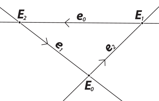
Figure 8: Fundamental triangle of coordinate system.

A perspective figure of the basis elements is shown in Fig. 8. The basis 1-vector $\mathbf{e}_{0}$ represents the ideal line, sometimes called the “line at infinity” and written $\omega$ to remind us that it is defined in a coordinate-free way. $\mathbf{e}_{1}$ and $\mathbf{e}_{2}$ represent the coordinate lines $x=0$ and $y=0$, resp. These basis vectors satisfy $\mathbf{e}_{0}^{2}=0$ and $\mathbf{e}_{1}^{2}=\mathbf{e}_{2}^{2}=1$, consistent with the signature $(2,0,1)$. Note that by orthogonality, $\mathbf{e}_{i}\mathbf{e}_{j}=\mathbf{e}_{i}\wedge\mathbf{e}_{j}$ when $i\neq j$. A basis for the 2-vectors is given by the products (i. e., intersection points) of these orthogonal basis lines:

$$\mathbf{E}_{0}:=\mathbf{e}_{1}\mathbf{e}_{2},\leavevmode\nobreak\ \leavevmode\nobreak\ \leavevmode\nobreak\ \mathbf{E}_{1}:=\mathbf{e}_{2}\mathbf{e}_{0},\leavevmode\nobreak\ \leavevmode\nobreak\ \leavevmode\nobreak\ \mathbf{E}_{2}:=\mathbf{e}_{0}\mathbf{e}_{1}$$

whereby $\mathbf{E}_{0}$ is the origin, $\mathbf{E}_{1}$ and $\mathbf{E}_{2}$ are the $x$- and $y-$ directions (ideal points), resp. They satisfy $\mathbf{E}_{0}^{2}=-1$ while $\mathbf{E}_{1}^{2}=\mathbf{E}_{2}^{2}=0$. That is, the signature on the 2-vectors is more degenerate: $(1,0,2)$. Finally, the unit pseudoscalar $\mathbf{I}:=\mathbf{e}_{0}\mathbf{e}_{1}\mathbf{e}_{2}$ represents the whole plane and satisfies $\mathbf{I}^{2}=0$. The full 8x8 multiplication table of these basis elements can be found in Table 2.

Exercise. 1) For a 1-vector $\mathbf{m}=a\mathbf{e}_{1}+b\mathbf{e}_{2}+c\mathbf{e}_{0}$, $\mathbf{m}^{2}=a^{2}+b^{2}$. 2) For a 2-vector $\mathbf{P}=x\mathbf{E}_{1}+y\mathbf{E}_{2}+z\mathbf{E}_{0}$, $\mathbf{P}^{2}=-z^{2}$.

	$\mathbf{1}$	$\mathbf{e}_{0}$	$\mathbf{e}_{1}$	$\mathbf{e}_{2}$	$\mathbf{E}_{0}$	$\mathbf{E}_{1}$	$\mathbf{E}_{2}$	$\mathbf{I}$
$\mathbf{1}$	$\mathbf{1}$	$\mathbf{e}_{0}$	$\mathbf{e}_{1}$	$\mathbf{e}_{2}$	$\mathbf{E}_{0}$	$\mathbf{E}_{1}$	$\mathbf{E}_{2}$	$\mathbf{I}$
$\mathbf{e}_{0}$	$\mathbf{e}_{0}$	$0$	$\mathbf{E}_{2}$	$-\mathbf{E}_{1}$	$\mathbf{I}$	$0$	$0$	$0$
$\mathbf{e}_{1}$	$\mathbf{e}_{1}$	$-\mathbf{E}_{2}$	$\mathbf{1}$	$\mathbf{E}_{0}$	$\mathbf{e}_{2}$	$\mathbf{I}$	$-\mathbf{e}_{0}$	$\mathbf{E}_{1}$
$\mathbf{e}_{2}$	$\mathbf{e}_{2}$	$\mathbf{E}_{1}$	$-\mathbf{E}_{0}$	$\mathbf{1}$	$-\mathbf{e}_{1}$	$\mathbf{e}_{0}$	$\mathbf{I}$	$\mathbf{E}_{2}$
$\mathbf{E}_{0}$	$\mathbf{E}_{0}$	$\mathbf{I}$	$-\mathbf{e}_{2}$	$\mathbf{e}_{1}$	$-\mathbf{1}$	$-\mathbf{E}_{2}$	$\mathbf{E}_{1}$	$-\mathbf{e}_{0}$
$\mathbf{E}_{1}$	$\mathbf{E}_{1}$	$0$	$\mathbf{I}$	$-\mathbf{e}_{0}$	$\mathbf{E}_{2}$	$0$	$0$	$0$
$\mathbf{E}_{2}$	$\mathbf{E}_{2}$	$0$	$\mathbf{e}_{0}$	$\mathbf{I}$	$-\mathbf{E}_{1}$	$0$	$0$	$0$
$\mathbf{I}$	$\mathbf{I}$	$0$	$\mathbf{E}_{1}$	$\mathbf{E}_{2}$	$-\mathbf{e}_{0}$	$0$	$0$	$0$

Table 2: Multiplication table for the geometric product in $\mathbf{P}(\mathbb{R}^{*}_{2,0,1})$

7.1 Normalizing $k$-vectors

From the previous exercise, the square of any $k$-vector is a scalar. When it is non-zero, the element is said to be euclidean, otherwise it is ideal. Just as with euclidean vectors in $\mathbb{R}^{n}$, it’s possible and often preferable to normalize simple $k$-vectors. Euclidean $k$-vectors can be normalized by the formula

$$\widehat{\mathbf{X}}:=\cfrac{\mathbf{X}}{\sqrt{|\mathbf{X}^{2}|}}$$

Then $\widehat{\mathbf{X}}$ satisfies $\mathbf{X}^{2}=\pm 1$.

For a euclidean line $\mathbf{a}$, the element $\widehat{\mathbf{a}}:=\dfrac{\mathbf{a}}{\sqrt{\mathbf{a}^{2}}}$ represents the same line but is normalized so that $\widehat{\mathbf{a}}^{2}=1$. A euclidean point $\mathbf{P}=x\mathbf{E}_{1}+y\mathbf{E}_{2}+\mathbf{E}_{0}$ is normalized and satisfies $\mathbf{P}^{2}=-1$. This gives rise to a standard norm on euclidean $k$-vectors $\mathbf{X}$ that we write $\|\mathbf{X}\|$.

7.1.1 The ideal norm

Such a normalization is not possible for ideal elements, since these satisfy $\mathbf{X}^{2}=0$. It turns out that there is a “natural” non-zero norm on ideal elements that arises by requiring that the inner product of any 2 $(n-1)$-dimensional ideal flats should be the same as the inner product between any two euclidean $n$-dimensional flats whose intersections with the ideal plane are these two ideal flats. For example, when $n=2$ this means that the inner product of ideal points is the same as the inner product of any pair of lines meeting the ideal line in these points. The reader can check that this is well-defined by recalling that moving a line parallel to itself does not change its angle to other lines.

If the two lines are $a_{i}\mathbf{e}_{1}+b_{i}\mathbf{e}_{2}+c_{i}\mathbf{e}_{0})$ their inner product is $(a_{0}a_{1}+b_{0}b_{1})$ and their ideal points are $a_{i}\mathbf{E}_{01}+b_{i}\mathbf{E}_{02}$. In order for the inner product of these two lines to be $(a_{0}a_{1}+b_{0}b_{1})$ it’s clear that the signature on the ideal line has to be $(2,0,0)$, and in general, $(n,0,0)$. In this way the set of ideal elements are given the structure of an $(n-1)$-dimensional dual PGA with signature $(n,0,0)$, the standard positive definite metric of $\mathbb{R}^{n}$: ideal points are identical with euclidean vectors, a fact already recognized by Clifford [Cli73]. In the projective setting we say that the ideal plane has an elliptic metric.

In fact, rather than starting with the euclidean planes and deducing the “induced” inner product on ideal lines as sketched above, it is also possible to start with this inner product on the ideal elements and “extend” it onto the euclidean elements (i. e., the inner product of two euclidean lines is defined to be the inner product of their two ideal points). This approach to the ideal norm is sketched in the appendix of [Gun17a].

In the case of $n-2$, this yields an ideal norm with the following properties.

• Point In terms of the coordinates introduced above, for an ideal point $\mathbf{V}=x\mathbf{E}_{1}+y\mathbf{E}_{2}$, $\|\mathbf{V}\|_{\infty}:=\sqrt{x^{2}+y^{2}}$. A coordinate-free definition of the ideal norm of an ideal point $\mathbf{V}$ is given by $\|\mathbf{V}\|_{\infty}:=\|\mathbf{V}\vee\mathbf{P}\|$ for any normalized euclidean point $\mathbf{P}$.

• Line The ideal norm for an ideal line $\mathbf{m}=c\mathbf{e}_{0}$ is given by $\|\mathbf{m}\|_{\infty}:=c$. This can be obtained in a coordinate-free way via the formula $\|\mathbf{m}\|_{\infty}=\mathbf{m}\vee\mathbf{P}$ where $\mathbf{P}$ is any normalized euclidean point. Using the $\vee$ operator instead of $\wedge$ produces a scalar directly instead of a pseudoscalar with the same numerical value.

• Pseudoscalar We can also consider the pseudoscalar as an ideal element since since $\mathbf{I}^{2}=0$. The ideal norm for a pseudoscalar $a\mathbf{I}$ is $\|a\mathbf{I}\|_{\infty}=a$.

Note that the ideal norms for lines and pseudoscalars are signed magnitudes. This is due to the fact that they belong to 1-dimensional subspaces that allow such a coordinate-free signed magnitude (based on the single generator). To distinguish them from traditional (non-negative) norms we call them numerical values but use the same notation $\|...\|_{\infty}$ for both.

7.1.2 Ideal norm via Poincaré duality

Another neat way to compute the ideal norm is provided by Poincaré duality. The discussion of Poincaré duality above in Sect. 5.10 took place at the level of the Grassmann algebra. It’s possible to consider this map to be between geometric algebras, in this case, $J:\mathbf{P}(\mathbb{R}^{*}_{2,0,1})\rightarrow\mathbf{P}(\mathbb{R}_{2,0,1})$. We leave it as an exercise for the reader to verify that for ideal $\mathbf{x}\in\mathbf{P}(\mathbb{R}^{*}_{2,0,1})$, $\|\mathbf{x}\|_{\infty}=\|J(\mathbf{x})\|$ (where by sleight-of-hand the scalar on the right-hand side is interpreted as a scalar in $\mathbf{P}(\mathbb{R}^{*}_{2,0,1})$). That is, the ideal norm in the euclidean plane is the ordinary norm in the dual euclidean plane. Naturally the same holds for arbitrary dimension. Whether this “trick” has a deeper meaning remains a subject of research.

We will see that the two norms – euclidean and ideal – harmonize remarkably with each other, producing polymorphic formulas – formulas that produce correct results for any combination of euclidean and ideal arguments. The sequel presents numerous examples.

Weight of a vector. Regardless of the type of norm, if an element satisfies $\|\mathbf{X}\|=d\in\mathbb{R}$, we say it has weight $d$. The normed elements have weight 1. A typical computation requires that the arguments are normalized; the weight of the result then gives important insight into the calculation. That means, we don’t work strictly projectively, but use the weight to distinguish between elements that are projectively equivalent. We will see this below, in the section on 2-way products. In the discussions below, we assume that all the arguments have been normalized with the appropriate norm since, just as in $\mathbb{R}^{n}$, it simplifies many formulas.

7.2 Examples: Products of pairs of elements in 2D

We get to know the geometric product better by considering basic products. We consider first multiplication by the pseudoscalar $\mathbf{I}$, then turn to products of pairs of normalized euclidean points and lines. It may be helpful to refer to the multiplication table (Table 2) while reading this section. Also, consult Fig. 9 which illustrates many of the products discussed below. A fuller discussion can be found in [Gun17a].

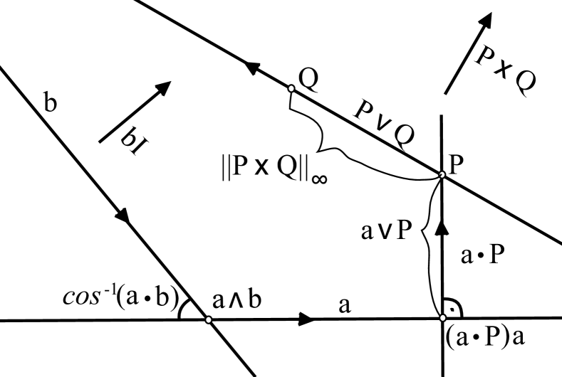
Figure 9: Selected geometric products of pairs of simple vectors.

Multiplication by the pseudoscalar. Multiplication by the pseudoscalar $\mathbf{I}$ maps a $k$-vector onto its orthogonal complement with respect to the euclidean metric. For a euclidean line $\mathbf{a}$, $\mathbf{a}^{\perp}:=\mathbf{a}\mathbf{I}$ is an ideal point perpendicular to the direction of $\mathbf{a}$. For a euclidean point $\mathbf{P}$, $\mathbf{P}^{\perp}:=\mathbf{P}\mathbf{I}$ is the ideal line $\mathbf{e}_{0}$. Multiplication by $\mathbf{I}$ is also called the polarity on the metric quadric, or just the polarity operator.

Product of two euclidean lines. We saw above that this product can be used as the starting point for the geometric product:

$$\mathbf{a}\mathbf{b}=\mathbf{a}\cdot\mathbf{b}+\mathbf{a}\wedge\mathbf{b}$$

$\mathbf{a}\cdot\mathbf{b}=\langle\mathbf{a}\mathbf{b}\rangle_{0}=\cos{\alpha}$, where $\alpha$ is the oriented angle between the two lines ($\pm 1$ when they coincide or are parallel), while $\mathbf{a}\wedge\mathbf{b}=\langle\mathbf{a}\mathbf{b}\rangle_{2}$ is their intersection point. If we call the normalized intersection point $\mathbf{P}$ (using the appropriate norm), then $\langle\mathbf{a}\mathbf{b}\rangle_{2}=(\sin{\alpha})\mathbf{P}$ when the lines intersect and $\langle\mathbf{a}\mathbf{b}\rangle_{2}=d_{ab}\mathbf{P}$ when the lines are parallel and are separated by a distance $d_{ab}$. Here we see the remarkable functional polymorphism mentioned earlier, reflecting the harmonious interaction of the two norms.

Product of two euclidean points.

$$\mathbf{P}\mathbf{Q}=\langle\mathbf{P}\mathbf{Q}\rangle_{0}+\langle\mathbf{P}\mathbf{Q}\rangle_{2}=-1+d_{PQ}\mathbf{V}$$

The inner product of any two normalized euclidean points is -1. This illustrates the degeneracy of the metric on points: every other point yields the same inner product with a given point! The grade-2 part is more interesting: it is the direction (ideal point) perpendicular to the joining line $\mathbf{P}\vee\mathbf{Q}$. It’s easy to verify that $\langle\mathbf{P}\mathbf{Q}\rangle_{2}=\mathbf{P}\times\mathbf{Q}$. $\mathbf{V}$ in the formula is the normalized form of $\mathbf{P}\times\mathbf{Q}$. Then the formula shows that the distance $d_{PQ}$ between the two points satisfies $d_{PQ}=\|\mathbf{P}\times\mathbf{Q}\|_{\infty}$: while the inner product of two points cannot be used to obtain their distance, $\langle\mathbf{P}\mathbf{Q}\rangle_{2}$ can. Here are two further formulas that yield this distance: $d_{PQ}=\|\mathbf{P}\vee\mathbf{Q}\|=\|\mathbf{P}-\mathbf{Q}\|_{\infty}$.

Product of euclidean point and euclidean line. This yields a line and a pseudoscalar, both of which contain important geometric information:

$$\mathbf{a}\mathbf{P}=\langle\mathbf{a}\mathbf{P}\rangle_{1}+\langle\mathbf{a}\mathbf{P}\rangle_{3} =\mathbf{a}\cdot\mathbf{P}+\mathbf{a}\wedge\mathbf{P}$$

$$=\mathbf{a}_{P}^{\perp}+d_{aP}\mathbf{I}$$

Here $\mathbf{a}_{P}^{\perp}:=\mathbf{a}\cdot\mathbf{P}$ is the line passing through $\mathbf{P}$ perpendicular to $\mathbf{a}$, while the pseudoscalar part has weight $d_{aP}$, the euclidean distance between the point and the line. Note that this inner product is anti-symmetric: $\mathbf{P}\cdot\mathbf{a}=-\mathbf{a}\cdot\mathbf{P}$.

Practice in thinking dually: more about $\mathbf{a}\cdot\mathbf{P}$. You might be wondering, why is $\mathbf{a}\cdot\mathbf{P}$ a line through $\mathbf{P}$ perpendicular to $\mathbf{a}$? This is a good opportunity to practice thinking in the dual algebra. We are used to thinking of lines as being composed of points. That however is only valid in the standard algebra $\mathbf{P}(G)$. In the dual algebra, we have to think of points as being composed of lines! The 1-vectors (lines) are the building blocks; they create points via the meet operator. A point “consists” of the lines that pass through it – called the line pencil in $\mathbf{P}$. This is analogous to thinking of a line as consisting of all the points that lie on it – called the point range on the line. Consider $\mathbf{a}\cdot\mathbf{P}$ in this light.

When $\mathbf{P}$ lies on $\mathbf{a}$ then we can write $\mathbf{P}=\mathbf{a}\mathbf{b}$ for the orthogonal line $\mathbf{b}$ through $\mathbf{P}$. Then $\mathbf{a}\mathbf{P}=\mathbf{a}\mathbf{a}\mathbf{b}=\mathbf{b}$ since $\mathbf{a}^{2}=1$. Hence the claim is proven. When $\mathbf{P}$ does not lie on $\mathbf{a}$ the multiplication removes the line through $\mathbf{P}$ parallel to $\mathbf{a}$ from the grade-1 part of the product, leaving as before the line $\mathbf{b}$ orthogonal to $\mathbf{a}$. We leave the details as an exercise for the reader. (Hint: any line parallel to $\mathbf{a}$ is of the form $\mathbf{a}+k\mathbf{e}_{0}$.) This example shows why the inner product is often called a contraction since it reduces the dimension by removing common subspaces.

Remarks regarding 2-way products. In the above results, you can also allow one or both of the arguments to be ideal; one obtains in all cases meaningful, “polymorphic” results. We leave this as an exercise for the interested reader. Interested readers can consult [Gun17a]. The above formulas have been collected in Table 3. Note that the formulas assume normalized arguments.

After this brief excursion into the world 2-way products, we turn our attention to 3-way products with a repeated factor. First, we look at products of the form $\mathbf{XXY}$ (where $\mathbf{X}$ and $\mathbf{Y}$ are either $1$- or $2$-vectors). Applying the associativity of the geometric product produces “formula factories”, yielding a wide variety of important geometric identities. Secondly, products of the form $\mathbf{aba}$ for 1-vectors $\mathbf{a}$ and $\mathbf{b}$ are used to develop an elegant representation of euclidean motions in PGA based on so-called sandwich operators. [Gun17a] contains more about general 3-way products in $\mathbf{P}(\mathbb{R}^{*}_{2,0,1})$.

7.3 Formula factories through associativity

First recall that for a normalized euclidean point or line, $\mathbf{X}^{2}=\pm 1$. Use this and associativity to write

$$\mathbf{Y}=\pm(\mathbf{X}\mathbf{X})\mathbf{Y}=\pm\mathbf{X}(\mathbf{X}\mathbf{Y})$$

where $\mathbf{Y}$ is also a normalized euclidean $1$- or $2$-vector. The right-hand side yields an orthogonal decomposition of $\mathbf{Y}$ in terms of $\mathbf{X}$. Associativity of the geometric product shows itself here to be a powerful tool. These decompositions are not only useful in their own right, they provide the basis for a family of other constructions, for example, “the point on a given line closest to a given point”, or “the line through a given point parallel to a given line” (see also Table 3).

Note that the grade of the two vectors can differ. We work out below three orthogonal projections. As in the above discussions, we assume the given points and lines have been normalized, so their coefficients carry unambiguous metric information.

   

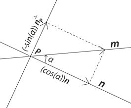
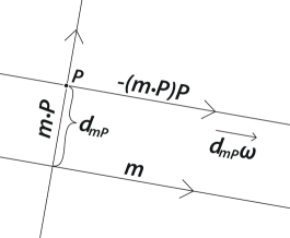
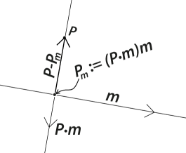
Figure 10: Orthogonal projections (l. to r.):, line $\mathbf{m}$ onto line $\mathbf{n}$, line $\mathbf{m}$ onto point $\mathbf{P}$, point $\mathbf{P}$ onto line $\mathbf{m}$.

Project line onto line. Assume both lines are euclidean and they they intersect in a euclidean point. Multiply

$$\mathbf{m}\mathbf{n}=\mathbf{m}\cdot\mathbf{n}+\mathbf{m}\wedge\mathbf{n}$$

with $\mathbf{n}$ on the right and use $\mathbf{n}^{2}=1$ to obtain

$$\mathbf{m} =(\mathbf{m}\cdot\mathbf{n})\mathbf{n}+(\mathbf{m}\wedge\mathbf{n})\mathbf{n}$$

$$=(\cos{\alpha})\mathbf{n}+(\sin{\alpha})\mathbf{P}\mathbf{n}$$

$$=(\cos{\alpha})\mathbf{n}-(\sin{\alpha})\mathbf{n}^{\perp}_{\mathbf{P}}$$

In the second line, $\mathbf{P}$ is the normalized intersection point of the two lines. Thus one obtains a decomposition of $\mathbf{m}$ as the linear combination of $\mathbf{n}$ and the perpendicular line $\mathbf{n}^{\perp}_{\mathbf{P}}$ through $\mathbf{P}$. See Fig. 10, left.

Exercise. If the lines are parallel one obtains $\mathbf{m}=\mathbf{n}+d_{\mathbf{m}\mathbf{n}}\omega$.

Project line onto point. Multiply $\mathbf{m}\mathbf{P}=\mathbf{m}\cdot\mathbf{P}+\mathbf{m}\wedge\mathbf{P}$ with $\mathbf{P}$ on the right and use $\mathbf{P}^{2}=-1$ to obtain

$$\mathbf{m} =-(\mathbf{m}\cdot\mathbf{P})\mathbf{P}-(\mathbf{m}\wedge\mathbf{P})\mathbf{P}$$

$$=-\mathbf{m}^{\perp}_{\mathbf{P}}\mathbf{P}-(d_{\mathbf{m}\mathbf{P}}\mathbf{I})\mathbf{P}$$

$$=\mathbf{m}^{||}_{\mathbf{P}}-d_{\mathbf{m}\mathbf{P}}\mathbf{\omega}$$

In the third equation, $\mathbf{m}^{||}_{\mathbf{P}}$ is the line through $\mathbf{P}$ parallel to $\mathbf{m}$, with the same orientation. Thus one obtains a decomposition of $\mathbf{m}$ as the sum of a line through $\mathbf{P}$ parallel to $\mathbf{m}$ and a multiple of the ideal line. Note that just as adding an ideal point (“vector”) to a point translates the point, adding an ideal line to a line translates the line. See Fig. 10, middle.

Project point onto line. Finally one can project a point $\mathbf{P}$ onto a line $\mathbf{m}$. One obtains thereby a decomposition of $\mathbf{P}$ as $\mathbf{P}_{m}$, the point on $\mathbf{m}$ closest to $\mathbf{P}$, plus a vector perpendicular to $\mathbf{m}$. See Fig. 10, right.

7.4 Representing isometries as sandwiches

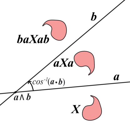
Figure 11: The reflection in the line $\mathbf{a}$ followed by reflection in line $\mathbf{b}$.

Three-way products of the form $\mathbf{a}\mathbf{b}\mathbf{a}$ for euclidean 1-vectors $\mathbf{a}$ and $\mathbf{b}$ turn out to represent the reflection of the line $\mathbf{b}$ in the line $\mathbf{a}$, and form the basis for an elegant realization of euclidean motions as sandwich operators. We sketch this here.

Let $\mathbf{a}$ and $\mathbf{b}$ be normalized 1-vectors representing different lines. Then

$$\mathbf{a}\mathbf{b}\mathbf{a} =\mathbf{a}(\mathbf{b}\mathbf{a})=\mathbf{a}(\mathbf{b}\cdot\mathbf{a}+\mathbf{b}\wedge\mathbf{a})$$

$$=\cos(\alpha)\mathbf{a}+\mathbf{a}(\mathbf{b}\wedge\mathbf{a})$$

$$=\cos(\alpha)\mathbf{a}+\sin(\alpha)\mathbf{a}\mathbf{P}$$

$$=\cos(\alpha)\mathbf{a}+\sin(\alpha)\mathbf{a}\cdot\mathbf{P}$$

$$=\cos(\alpha)\mathbf{a}+\sin(\alpha)\mathbf{a}^{\perp}_{\mathbf{P}}$$

We use the symmetry of the inner product in line 2. In line 3 we replace $\mathbf{a}\wedge\mathbf{b}$ with the normalized point $\mathbf{P}$ and weight $\sin{\alpha}$. Line 4 is justified by the fact that $\mathbf{a}\wedge\mathbf{P}=0$, and line 5 uses the definition of $\mathbf{a}^{\perp}_{\mathbf{P}}$. Compare this with the orthogonal decomposition for $\mathbf{b}$ obtained above in Sect. 10:

$$\mathbf{b}=\cos(\alpha)\mathbf{a}-\sin(\alpha)\mathbf{a}^{\perp}_{\mathbf{P}}$$

Using the fact that $\mathbf{a}^{\perp}_{\mathbf{P}}$ is a line perpendicular to $\mathbf{a}$ leads to the conclusion that $\mathbf{a}\mathbf{b}\mathbf{a}$ must be the reflection of $\mathbf{b}$ in $\mathbf{a}$, since the reflection in $\mathbf{a}$ is the unique linear map fixing $\mathbf{a}$ and $\omega$ and mapping $\mathbf{a}^{\perp}_{\mathbf{P}}$ to $-\mathbf{a}^{\perp}_{\mathbf{P}}$. (Exercise Prove that $\mathbf{a}\omega\mathbf{a}=-\omega$.) We call this the sandwich operator corresponding to $\mathbf{a}$ since $\mathbf{a}$ appears on both sides of the expression. It’s not hard to show that for a euclidean point $\mathbf{P}$, $\mathbf{a}\mathbf{P}\mathbf{a}$ is the reflection of $\mathbf{P}$ in the line $\mathbf{a}$. Similar results apply in higher dimensions: the same sandwich form for a reflection works regardless of the grade of the “meat” of the sandwich.

Operation	PGA
Intersection point of two lines	$\mathbf{a}\wedge\mathbf{b}$
Angle of two intersecting lines	$\cos^{-1}(\mathbf{a}\cdot\mathbf{b})$
	$\sin^{-1}(\|\mathbf{a}\wedge\mathbf{b}\|)$
Distance of two $||$ lines	$\|\mathbf{a}\wedge\mathbf{b}\|_{\infty}$
Joining line of two points	$\mathbf{P}\vee\mathbf{Q}$
$\perp$ direction to join of two points	$\mathbf{P}\times\mathbf{Q}$
Distance between two points	$\|\mathbf{P}\vee\mathbf{Q}\|$,$\leavevmode\nobreak\ \leavevmode\nobreak\ \|\mathbf{P}\times\mathbf{Q}\|_{\infty}$
Oriented distance point to line	$\|\mathbf{a}\wedge\mathbf{P}\|$
Angle of ideal point to line	$\sin^{-1}{(\|\mathbf{a}\wedge\mathbf{P}\|_{\infty})}$
Line through point $\perp$ to line	$\mathbf{P}\cdot\mathbf{a}$
Nearest point on line to point	$(\mathbf{P}\cdot\mathbf{a})\mathbf{a}$
Line through point $||$ to line	$(\mathbf{P}\cdot\mathbf{a})\mathbf{P}$
Oriented area of triangle $ABC$	$\frac{1}{2}(\mathbf{A}\vee\mathbf{B}\vee\mathbf{C})$
Length of closed loop $\mathbf{P}_{1}\mathbf{P}_{2}...\mathbf{P}_{n}$	$\Sigma_{i=1}^{n}\|\mathbf{P}_{i}\vee\mathbf{P}_{i+1}\|$
Oriented area of closed loop $\mathbf{P}_{1}\mathbf{P}_{2}...\mathbf{P}_{n}$	$\|\Sigma_{i=1}^{n}(\mathbf{P}_{i}\vee\mathbf{P}_{i+1})\|$
Reflection in line ($\mathbf{X}=$ point or line)	$\mathbf{a}\mathbf{X}\mathbf{a}$
Rotation around point of angle $2\alpha$	$\mathbf{R}\mathbf{X}\widetilde{\mathbf{R}}\leavevmode\nobreak\ \leavevmode\nobreak\ (\mathbf{R}:=e^{\alpha\mathbf{P}}$)
Translation by $2d$ in direction $\mathbf{V}^{\perp}$	$\mathbf{T}\mathbf{X}\widetilde{\mathbf{T}}\leavevmode\nobreak\ \leavevmode\nobreak\ (\mathbf{T}:=1+d{\mathbf{V}})$
Motor moving line $\mathbf{a}_{1}$ to $\mathbf{a}_{2}$	$1+\widehat{\mathbf{a}_{2}\mathbf{a}_{1}}$
Logarithm of motor $\mathbf{g}$	$\cos^{-1}(\langle\mathbf{g}\rangle_{0})\widehat{\langle\mathbf{g}\rangle_{2}}$

Table 3: A sample of geometric constructions and formulas in the euclidean plane using PGA (assuming normalized arguments, all arguments euclidean unless otherwise stated).

Rotations and translations. It is well-known that all isometries of euclidean space are generated by reflections. The sandwich $\mathbf{b}(\mathbf{a}\mathbf{X}\mathbf{a})\mathbf{b}$ represents the composition of reflection in line $\mathbf{a}$ followed by reflection in line $\mathbf{b}$. See Fig. 11. When the lines meet at angle $\frac{\alpha}{2}$, this is well-known to be a rotation around the point $\mathbf{P}$ through of angle $\alpha$. $\mathbf{R}:=\mathbf{a}\mathbf{b}=\cos{\frac{\alpha}{2}}+\sin{\frac{\alpha}{2}}\mathbf{P}$ by the above formula. The rotation can be expressed as $\mathbf{R}\mathbf{X}\widetilde{\mathbf{R}}$. (Here, $\widetilde{\mathbf{R}}$ is the reversal of $\mathbf{R}$, obtained by writing all products in the reverse order. When $\mathbf{R}$ is normalized, it’s also the inverse of $\mathbf{R}$.)

When $\mathbf{a}$ and $\mathbf{b}$ are parallel, $\mathbf{R}$ generates the translation in the direction perpendicular to the two lines, of twice the distance between them – once again, PGA polymorphism in action. A product of $k$ euclidean 1-vectors is called a $k$-versor; hence the sandwich operator is sometimes called a versor form for the isometry. When $\mathbf{R}$ is normalized so that $\mathbf{R}\widetilde{\mathbf{R}}=1$, it’s called a motor. A motor is either a rotator (when its fixed point is euclidean) or a translator (when it’s ideal).

Exponential form for motors. Motors can be generated directly from the normalized center point $\mathbf{P}$ and angle of rotation $\alpha$ using the exponential form

$$\mathbf{R}=e^{\frac{\alpha}{2}\mathbf{P}}=\cos{\frac{\alpha}{2}}+\sin{\frac{\alpha}{2}}\mathbf{P}$$

. This is another standard technique in geometric algebra: The exponential behaves like the exponential of a complex number since, as we noted above, a normalized euclidean point satisfies $\mathbf{P}^{2}=-1$. When $\mathbf{P}$ is ideal ($\mathbf{P}^{2}=0$), the same process yields a translation through distance $d$ perpendicular to the direction of $\mathbf{P}$, by means of the formula $\mathbf{T}=e^{\frac{d}{2}\mathbf{P}}=1+\frac{d}{2}\mathbf{P}$.

Motor moving one line to another. Given two lines $\mathbf{l}_{1}$ and $\mathbf{l}_{2}$, there is a unique direct isometry that moves $\mathbf{l}_{1}$ to $\mathbf{l}_{2}$ and fixes their intersection point $\mathbf{P}:=\mathbf{l}_{1}\wedge\mathbf{l}_{2}$. Indeed, we know that when $\mathbf{P}$ is euclidean and the angle of intersection is $\alpha$, the product $\mathbf{g}:=\mathbf{l}_{2}\mathbf{l}_{1}$ is a motor that rotates by $2\alpha$ around the intersection point $\mathbf{l}_{1}\wedge\mathbf{l}_{2}$. Hence the desired motor can be written $\sqrt{\mathbf{g}}$. (Exercise. When $\mathbf{g}$ has been normalized to satisfy $\|\mathbf{g}\|=1$, then $\sqrt{\mathbf{g}}=\widehat{1+\mathbf{g}}$. [Hint: The proof is similar to that of the statement: Given $P=(\cos{t},\sin{t})$ and $Q=(1,0)$ on the unit circle, $\dfrac{P+Q}{2}$ lies on the angle bisector of central angle $POQ$.]) This result is true also when $\mathbf{P}$ is ideal.

This concludes our treatment of the euclidean plane.Table 3 contains an overview of formulas available in $\mathbf{P}(\mathbb{R}^{*}_{2,0,1})$, most of which have been introduced in the above discussions. We are not aware of any other frameworks offering comparably concise and polymorphic formulas for plane geometry.

8 PGA for euclidean space: $\mathbf{P}(\mathbb{R}^{*}_{3,0,1})$

If you have followed the treatment of plane geometry using PGA, then you are well-prepared to tackle the 3D version $\mathbf{P}(\mathbb{R}^{*}_{3,0,1})$. Naturally in 3D one has points, lines, and planes, with the planes taking over the role of lines in 2D (as dual to points); the lines represent a new, middle element not present in 2D. With a little work one can derive similar results to the ones given above for 2-way products, for orthogonal decompositions, and for isometries. For example, $\mathbf{a}\cdot\mathbf{b}$ is the angled between two planes $\mathbf{a}$ and $\mathbf{b}$. A look at the tables of formulas for 3D (Table 4, Table 5) confirms that many of the 2D formulas reappear, with planes substituting for lines. If you re-read Examples 4.3 and 4.4 now you should understand much better how 3D isometries are represented in PGA, based on what you’ve learned about 2D sandwiches.

Notation and foundations. We continue to use large roman letters for points. Dual to points, planes are now written with small roman letters. Lines (and in general 2-vectors) are written with large Greek letters. Now $\mathbf{e}_{0}$ is an ideal plane instead of ideal line, and there are three ideal points $\mathbf{E}_{1}$, $\mathbf{E}_{2}$ and $\mathbf{E}_{3}$ representing the $x$-, $y$-, and $z$-directions instead of just three. Bivectors have 6 coordinates corresponding to the six intersection lines of the four basis planes. The lines $\mathbf{e}_{01},\mathbf{e}_{02},\mathbf{e}_{03}$ are ideal lines, and represent the intersections of the 3 euclidean basis planes with the ideal plane. The lines $\mathbf{e}_{23},\mathbf{e}_{31},\mathbf{e}_{12}$ are lines through the origin in the $(x,y,z)$-directions, resp. Hence, every bivector can be trivially written as the sum of an ideal line and a line through the origin.

In the interests of space, we leave it to the reader to confirm the similarities of the 3D case to the 2D case. We focus our energy for the remainder of this section on one important difference to 2D: bivectors of $\mathbf{P}(\mathbb{R}^{*}_{3,0,1})$, which, as we mentioned above, have no direct analogy in $\mathbf{P}(\mathbb{R}^{*}_{2,0,1})$.

Operation	formula
Intersection line of two planes	$\mathbf{a}\wedge\mathbf{b}$
Angle of two intersecting planes	$\cos^{-1}(\mathbf{a}\cdot\mathbf{b})$
	$\sin^{-1}(\|\mathbf{a}\wedge\mathbf{b}\|)$
Distance of two $||$ planes	$\|\mathbf{a}\wedge\mathbf{b}\|_{\infty}$
Joining line of two points	$\mathbf{P}\vee\mathbf{Q}$
Intersection point of three planes	$\mathbf{a}\wedge\mathbf{b}\wedge\mathbf{c}$
Joining plane of three points	$\mathbf{P}\vee\mathbf{Q}\vee\mathbf{R}$
Intersection of line and plane	${\mathbf{\Omega}}\wedge\mathbf{a}$
Joining plane of point and line	$\mathbf{P}\vee{\mathbf{\Omega}}$
Distance from point to plane	$\|\mathbf{a}\wedge\mathbf{P}\|$
Angle of ideal point to plane	$\sin^{-1}{(\|\mathbf{a}\wedge\mathbf{P}\|_{\infty})}$
$\perp$ line to join of two points	$\mathbf{P}\times\mathbf{Q}$
Distance of two points	$\|\mathbf{P}\vee\mathbf{Q}\|$,$\leavevmode\nobreak\ \leavevmode\nobreak\ \|\mathbf{P}\times\mathbf{Q}\|_{\infty}$
Line through point $\perp$ to plane	$\mathbf{P}\cdot\mathbf{a}$
Project point onto plane	$(\mathbf{P}\cdot\mathbf{a})\mathbf{a}$
Project plane onto point	$(\mathbf{P}\cdot\mathbf{a})\mathbf{P}$
Plane through line $\perp$ to plane	${\mathbf{\Omega}}\cdot\mathbf{a}$
Project line onto plane	$({\mathbf{\Omega}}\cdot\mathbf{a})\mathbf{a}$
Project plane onto line	$({\mathbf{\Omega}}\cdot\mathbf{a}){\mathbf{\Omega}}$
Plane through point $\perp$ to line	$\mathbf{P}\cdot{\mathbf{\Omega}}$
Project point onto line	$(\mathbf{P}\cdot{\mathbf{\Omega}}){\mathbf{\Omega}}$
Project line onto point	$(\mathbf{P}\cdot{\mathbf{\Omega}})\mathbf{P}$
Line through point $\perp$ to line	$((\mathbf{P}\cdot{\mathbf{\Omega}}){\mathbf{\Omega}})\vee\mathbf{P}$
Oriented volume of tetrahedron $ABCD$	$\frac{1}{3}\|\mathbf{A}\vee\mathbf{B}\vee\mathbf{C}\vee\mathbf{D}\|$
Area of triangle mesh $M$	$\frac{1}{2}\sum\limits_{\Delta_{i}\in M}\|\hat{\mathbf{P}}_{i1}\vee\hat{\mathbf{P}}_{i2}\vee\hat{\mathbf{P}}_{i3}\|$
Volume of closed triangle mesh $M$	$\frac{1}{3}\|(\sum\limits_{\Delta_{i}\in M}\hat{\mathbf{P}}_{i1}\vee\hat{\mathbf{P}}_{i2}\vee\hat{\mathbf{P}}_{i3})\|_{\infty}$

Table 4: A sample of geometric constructions and formulas in 3D using PGA (assuming normalized arguments).

Operation	formula
Common normal line to $\mathbf{\Omega}_{1},\mathbf{\Omega}_{2}$	$\widehat{\mathbf{\Omega}_{1}\times\mathbf{\Omega}_{2}}$
Angle $\alpha$ between $\mathbf{\Omega}_{1},\mathbf{\Omega}_{2}$	$\alpha=\cos^{-1}{(\hat{\mathbf{\Omega}}_{1}\cdot\hat{\mathbf{\Omega}}_{2})}$
Distance between $\mathbf{\Omega}_{1},\mathbf{\Omega}_{2}$	$d_{\mathbf{\Omega}_{1}\mathbf{\Omega}_{2}}={\csc{\alpha}\,{(\hat{\mathbf{\Omega}}_{1}\vee\hat{\mathbf{\Omega}}_{2})}}$
Refl. in plane ($\mathbf{X}=$ pt, ln, or pl)	$\mathbf{a}\mathbf{X}\mathbf{a}$
Rotation with axis ${\mathbf{\Omega}}$ by angle $2\alpha$	$\mathbf{R}\mathbf{X}\widetilde{\mathbf{R}}\leavevmode\nobreak\ \leavevmode\nobreak\ (\mathbf{R}:=e^{\alpha{\mathbf{\Omega}}}$)
Translation by $2d$ in direction $\mathbf{V}$	$\mathbf{T}\mathbf{X}\widetilde{\mathbf{T}}\leavevmode\nobreak\ \leavevmode\nobreak\ (\mathbf{T}:={(\mathbf{E}_{0}\vee d\mathbf{V})\mathbf{I}})$
Screw with axis ${\mathbf{\Omega}}$ and pitch $p$	$\mathbf{S}\mathbf{X}\widetilde{\mathbf{S}}\leavevmode\nobreak\ \leavevmode\nobreak\ (\mathbf{S}:=e^{t(1+p\mathbf{I}){\mathbf{\Omega}}})$
Logarithm of motor $\mathbf{m}$	$\mathbf{b}=\langle\mathbf{m}\rangle_{2},s=\sqrt{-\mathbf{b}\cdot\mathbf{b}},p=\frac{-\mathbf{b}\wedge\mathbf{b}}{2s}$
	$\widehat{\mathbf{b}}=\frac{s-p}{s^{2}}\mathbf{b}$
	$\log\mathbf{m}=\big{(}\tan^{-1}(\frac{s}{\langle\mathbf{m}\rangle_{0}})+\frac{p}{\langle\mathbf{m}\rangle_{0}}\big{)}\widehat{\mathbf{b}}$

Table 5: More formulas in 3D using PGA focused on motors and bivectors.

8.1 Simple and non-simple bivectors in 3D

In $\mathbf{P}(\mathbb{R}^{*}_{2,0,1})$, all $k$-vectors are simple, that is, they can be written as the product of $k$ 1-vectors. This is no longer the case in $\mathbf{P}(\mathbb{R}^{*}_{3,0,1})$. A simple bivector ${\mathbf{\Sigma}}$ in 3D is the geometric product of two perpendicular planes ${\mathbf{\Sigma}}=\mathbf{p}_{1}\wedge\mathbf{p}_{2}$ and represents their intersection line. Then clearly ${\mathbf{\Sigma}}\wedge{\mathbf{\Sigma}}=0$. Let ${\mathbf{\Sigma}}_{1}$ and ${\mathbf{\Sigma}}_{2}$ be two simple bivectors that represent skew lines. We claim that the bivector sum ${\mathbf{\Sigma}}:={\mathbf{\Sigma}}_{1}+{\mathbf{\Sigma}}_{2}$ is a non-simple. First note that since ${\mathbf{\Sigma}}_{1}$ and ${\mathbf{\Sigma}}_{2}$ are skew, they are linearly independent, implying ${\mathbf{\Sigma}}_{1}\wedge{\mathbf{\Sigma}}_{2}\neq 0$. Then, using bilinearity and symmetry of the wedge product (on bivectors!), one obtains directly ${\mathbf{\Sigma}}\wedge{\mathbf{\Sigma}}=2{\mathbf{\Sigma}}_{1}\wedge{\mathbf{\Sigma}}_{2}\neq 0$. We saw above however that a simple 2-vector ${\mathbf{\Sigma}}$ satisfies ${\mathbf{\Sigma}}\wedge{\mathbf{\Sigma}}=0$. Hence ${\mathbf{\Sigma}}$ must be non-simple. In fact, as the next section shows, most bivectors are non-simple.

Exponentials of simple bivectors. In the sequel we will need to know the exponential of a simple bivector. The situation is exactly analogous to the 2D case handled above and yields: For a simple euclidean bivector ${\mathbf{\Omega}}$, $e^{\alpha}{\mathbf{\Omega}}=\cos{\alpha}+\sin{\alpha}{\mathbf{\Omega}}$. For a simple ideal bivector ${\mathbf{\Omega}}_{\infty}$, $e^{d{\mathbf{\Omega}}_{\infty}}=1+d{\mathbf{\Omega}}_{\infty}$.

8.1.1 The space of bivectors and Plücker’s line quadric

As noted above, the space of bivectors $\bigwedge^{2}$ is spanned by the 6 basis elements $\mathbf{e}_{ij}:=\mathbf{e}_{i}\mathbf{e}_{j}$ and forms a 5-dimensional projective space $\mathbf{P}(\bigwedge^{2})$. From the above discussion we can see the condition that a bivector ${\mathbf{\Omega}}$ is a line can be written as ${\mathbf{\Omega}}\wedge{\mathbf{\Omega}}=0$. (In terms of coordinates, the bivector $\Sigma a_{ij}\mathbf{e}_{ij}$ is a line $\iff$ $a_{01}a_{23}+a_{02}a_{31}+a_{03}a_{12}=0$.) This defines the Plücker quadric $\mathcal{L}$, a 4D quadric surface (with signature $(3,3,0)$) sitting inside $\mathbf{P}(\bigwedge^{2})$, and giving rise to the well-known Plücker coordinates for lines. Points not on the quadric are non-simple bivectors, also known as linear line complexes. Consult Figure 12. Linear line complexes were first introduced by [Möb37] in his early studies of statics under the name null systems.

8.1.2 Product of two euclidean lines

Here we present an account of the geometric product of two euclidean lines. Justifications for the claims made can be found in the subsequent sections. Let the two lines be ${\mathbf{\Omega}}$ and ${\mathbf{\Sigma}}$. Assume they are euclidean and normalized, i.e., ${\mathbf{\Omega}}\wedge{\mathbf{\Sigma}}\neq 0$ and ${\mathbf{\Omega}}^{2}={\mathbf{\Sigma}}^{2}=-1$. Two euclidean lines determine in general a unique third euclidean line that is perpendicular to both, call it ${\mathbf{\Pi}}$. Consult Fig. 12, right. ${\mathbf{\Omega}}{\mathbf{\Sigma}}$ consists of 3 parts, of grades 0, 2, and 4:

$${\mathbf{\Omega}}{\mathbf{\Sigma}} =\langle{\mathbf{\Omega}}{\mathbf{\Sigma}}\rangle_{0}+\langle{\mathbf{\Omega}}{\mathbf{\Sigma}}\rangle_{2}+\langle{\mathbf{\Omega}}{\mathbf{\Sigma}}\rangle_{4}$$

$$={\mathbf{\Omega}}\cdot{\mathbf{\Sigma}}+{\mathbf{\Omega}}\times{\mathbf{\Sigma}}+{\mathbf{\Omega}}\wedge{\mathbf{\Sigma}}$$

$$=\cos{\alpha}+(\sin{\alpha}{\mathbf{\Pi}}+d\cos{\alpha}{\mathbf{\Pi}}^{\perp})+d\sin{\alpha}\mathbf{I}$$

$\alpha$ is the angle between ${\mathbf{\Omega}}$ and ${\mathbf{\Sigma}}$, viewed along the common normal ${\mathbf{\Pi}}$; $d$ is the distance between the two lines measured along ${\mathbf{\Pi}}$ (0 when the lines intersect). $d\sin{\alpha}$ is the volume of a tetrahedron determined by unit length segments on ${\mathbf{\Omega}}$ and ${\mathbf{\Sigma}}$. Finally, ${\mathbf{\Omega}}\times{\mathbf{\Sigma}}$ is a weighted sum of ${\mathbf{\Pi}}$ and ${\mathbf{\Pi}}^{\perp}$. The appearance of ${\mathbf{\Pi}}^{\perp}$ is not so surprising, as it is also a “common normal” to ${\mathbf{\Omega}}$ and ${\mathbf{\Sigma}}$, but as an ideal line, is easily overlooked.

Does ${\mathbf{\Omega}}{\mathbf{\Sigma}}$ have a geometric meaning? Consider sandwich operators with bivectors, that is, products of the form ${\mathbf{\Omega}}\mathbf{X}\widetilde{{\mathbf{\Omega}}}$ for simple euclidean ${\mathbf{\Omega}}$. Such a product is called a turn since it is a half-turn around the axis ${\mathbf{\Omega}}$ (see below, Sect. 8.1.5). And, in turn, the turns generate the full group $E^{+}(3)$ of direct euclidean isometries ([Stu91]. A little reflection shows that the composition of the two turns ${\mathbf{\Omega}}{\mathbf{\Sigma}}$ will be a screw motion that rotates around the common normal ${\mathbf{\Pi}}$ by $2\alpha$ while translating by $2d$ in the direction from ${\mathbf{\Sigma}}$ to ${\mathbf{\Omega}}$ (the translation is a “rotation” around ${\mathbf{\Pi}}^{\perp}$). This is analogous to the product of two reflections meeting at angle $\alpha$ discussed above in Sect. 7.4.

Analogous to the 2D case, we can easily calculate the motor that carries ${\mathbf{\Sigma}}$ exactly onto ${\mathbf{\Omega}}$. This is given by $\sqrt{{\mathbf{\Omega}}{\mathbf{\Sigma}}}=\widehat{\left(\cfrac{1+{\mathbf{\Omega}}{\mathbf{\Sigma}}}{2}\right)}$.

The case of two intersecting lines. If the two lines are not skew, they have a common point and a common plane and are linearly dependent: ${\mathbf{\Omega}}\wedge{\mathbf{\Sigma}}=0$. The common plane is given by $({\mathbf{\Omega}}\wedge\mathbf{e}_{0})\vee{\mathbf{\Sigma}}$; the common point $\mathbf{P}$ by $\mathbf{P}=(({\mathbf{\Pi}}\wedge\mathbf{e}_{0})\vee{\mathbf{\Omega}})\wedge{\mathbf{\Sigma}}$ where ${\mathbf{\Pi}}=\langle{\mathbf{\Omega}}{\mathbf{\Sigma}}\rangle_{2}$ is the common normal.

We turn now to a rather detailed discussion of the structure and behavior of non-simple bivectors. Readers with limited time and interest in such a treatment are encouraged to skip ahead to Sect. 9.

 

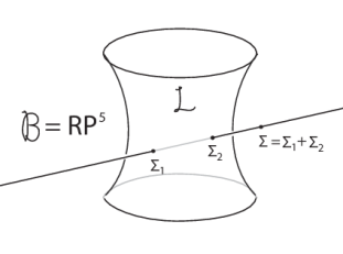
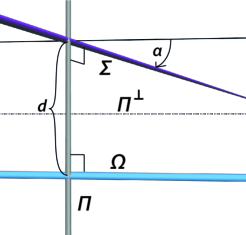
Figure 12: Left:The space of lines sits inside the space of 2-vectors as a quadric surface $\mathcal{L}$. Right: Product of two skew lines ${\mathbf{\Omega}}$ and ${\mathbf{\Sigma}}$ involving the common normals ${\mathbf{\Pi}}$ (euclidean) and ${\mathbf{\Pi}}^{\perp}$ (ideal).

8.1.3 The axis of a bivector

In 2D we used the following formula to normalize a 1- or 2-vector:

$$\widehat{\mathbf{X}}=\cfrac{\mathbf{X}}{\sqrt{|\mathbf{X}^{2}|}}$$

This was made easy since $\mathbf{X}^{2}$ in all cases was a real number. A non-simple euclidean bivector satisfies ${\mathbf{\Theta}}^{2}={\mathbf{\Theta}}\cdot{\mathbf{\Theta}}+{\mathbf{\Theta}}\wedge{\mathbf{\Theta}}=s+p\mathbf{I}$ with $s,p\neq 0$. Since it’s euclidean, $s<0$. We saw above in Sect. 8.1 that $p\neq 0\iff{\mathbf{\Theta}}$ is non-simple. A number of the form $s+p\mathbf{I}$ for $s,t\in\mathbb{R}$ is called a dual number. If we want to normalize a bivector using a formula like the one above, then we have to be able to find the square root of dual numbers.

For a dual number $d=s+p\mathbf{I},s>0,p\neq 0$, define the square root

$$\sqrt{s+p\mathbf{I}}=\sqrt{s}+\cfrac{p}{2\sqrt{s}}\mathbf{I}$$

and verify that it deserves the name. Define

$$\|{\mathbf{\Theta}}\|=u+v\mathbf{I}:=\sqrt{-({\mathbf{\Theta}}\cdot{\mathbf{\Theta}}+{\mathbf{\Theta}}\wedge{\mathbf{\Theta}}})$$

Then $\widehat{{\mathbf{\Theta}}}:=\|{\mathbf{\Theta}}\|^{-1}{\mathbf{\Theta}}$ and $\widehat{{\mathbf{\Theta}}}^{2}=-1$. We write ${\mathbf{\Theta}}$ in terms of $\widehat{{\mathbf{\Theta}}}$:

$${\mathbf{\Theta}} =\|{\mathbf{\Theta}}\|\widehat{{\mathbf{\Theta}}}=(u+v\mathbf{I})\widehat{{\mathbf{\Theta}}}$$

$$=u\widehat{{\mathbf{\Theta}}}+v\widehat{{\mathbf{\Theta}}}^{\perp}$$

That is, we have decomposed the non-simple bivector as the sum of a euclidean line $\widehat{{\mathbf{\Theta}}}$ and its orthogonal line $\widehat{{\mathbf{\Theta}}}^{\perp}$. It is easy to verify that $\widehat{{\mathbf{\Theta}}}\times\widehat{{\mathbf{\Theta}}}^{\perp}=0$ so that the two bivectors commute. We now apply this to computing the exponential of a bivector that we need below in Sect. 13.

Remarks on the axis pair. Note that $\widehat{{\mathbf{\Theta}}}$ is not a normalized vector in the traditional sense since it is no longer projectively equivalent to the original bivector. Indeed, it arises by multiplying the latter by a dual number, not a real number. The euclidean axis has a special geometric significance that will prove to be very useful in the analysis of motors that follows.

Terminology. We call $\widehat{{\mathbf{\Theta}}}$ the euclidean axis and $\widehat{{\mathbf{\Theta}}}^{\perp}$ the ideal axis of the non-simple bivector ${\mathbf{\Theta}}$. Together they form the axis pair of the bivector. The euclidean axis however is primary since the ideal axis can be obtained from it by polarizing: $\widehat{{\mathbf{\Theta}}}\mathbf{I}$, but not vice-versa.

8.1.4 The exponential of a non-simple bivector

The existence of an axis pair for an non-simple bivector is the key to understanding its exponential. Applying the decomposition of ${\mathbf{\Theta}}=u\widehat{{\mathbf{\Theta}}}+v\widehat{{\mathbf{\Theta}}}^{\perp}$ as an axis pair we can write

$$e^{{\mathbf{\Theta}}}=e^{v\widehat{{\mathbf{\Theta}}}+v\widehat{{\mathbf{\Theta}}}^{\perp}}$$

Since ${\mathbf{\Theta}}$ and ${\mathbf{\Theta}}^{\perp}$ commute (see above), the exponent of the sum is the product of the exponents:

$$e^{{\mathbf{\Theta}}}=e^{u\widehat{{\mathbf{\Theta}}}+v\widehat{{\mathbf{\Theta}}}^{\perp}}=e^{u\widehat{{\mathbf{\Theta}}}}e^{v\widehat{{\mathbf{\Theta}}}^{\perp}}=e^{v\widehat{{\mathbf{\Theta}}}^{\perp}}e^{u\widehat{{\mathbf{\Theta}}}}$$

where the third equality also follows from commutivity. We can then apply what we know about the exponential of simple bivectors from Sect. 8.1 to obtain:

$$e^{{\mathbf{\Theta}}} =(\cos{u}+\sin{u}\widehat{{\mathbf{\Theta}}})(1+v\widehat{{\mathbf{\Theta}}}\mathbf{I})$$ (1)

$$=\cos{u}+\sin{u}\widehat{{\mathbf{\Theta}}}+v\cos{u}\widehat{{\mathbf{\Theta}}}\mathbf{I}-v\sin{u}\mathbf{I}$$ (2)

$$=(\cos{u}-v\sin{u}\mathbf{I})+(\sin{u}+v\cos{u}\mathbf{I})\widehat{{\mathbf{\Theta}}}$$ (3)

We will apply this formula below when we compute the logarithm of a motor $\mathbf{m}$.

8.1.5 Bivectors and motions

Simple bivectors, simple motions. We saw in the discussion of 2D PGA that bivectors (points) play an important role in implementing euclidean motions: every rotation (translation) can be implemented by exponentiating a euclidean (ideal) point to obtain a motor. This was a consequence of the fact that sandwiches with 1-vectors (lines) implement reflections and even compositions of reflections generate all direct isometries. The same stays true in 3D: a sandwich with a plane (1-vector) implements the reflection in that plane. Composing two such reflections generates a direct motion (rotation/translation around the intersection line) that is represented by a 3D motor, completely analogous to the 2D case. Using the formula for the exponential of a simple bivector from Sect. 8.1, we derive the formulas for the rotator around a simple euclidean bivector ${\mathbf{\Omega}}$ by angle $\alpha$: $e^{\frac{\alpha}{2}{\mathbf{\Omega}}}=\cos{\frac{\alpha}{2}}+\sin{\frac{\alpha}{2}}{\mathbf{\Omega}}$. The translator $e^{\frac{d}{2}{\mathbf{\Omega}}_{\infty}}=1+\frac{d}{2}{\mathbf{\Omega}}_{\infty}$ produces a translation of length $d$ perpendicular to the ideal line ${\mathbf{\Omega}}_{\infty}$.

Non-simple bivectors, screw motions. But there are other possibilities in 3D for direct motions than just rotations and translations. The generic motion is a screw motion that composes a rotation around a 3D line, called its axis, with a translation in the direction of the line. To be precise, the axis of a screw motion is the unique euclidean line fixed by the screw motion. The motion is further characterized by its pitch, which is the ratio of the angle turned (in radians) to the distance translated.

8.1.6 The motor group

Every direct isometry is the result of composing an even number of reflections: hence such a motor lies in the even sub-subalgebra, consisting of elements of even grade and written $\mathbf{P}(\mathbb{R}^{*+}_{3,0,1})$. An element $\mathbf{m}$ of the even sub-algebra is a motor if it satisfies $\mathbf{m}\widetilde{\mathbf{m}}=1$; such elements form a group, written $\mathfrak{M}_{3,0,1}\subset\mathbf{P}(\mathbb{R}^{*+}_{3,0,1})$ called the motor group. The motor group is more generally called the Spin group of the geometric algebra. It’s a 2:1 cover of the direct Euclidean group $E^{+}(3)$ since $\mathbf{m}$ and $-\mathbf{m}$ yield the same isometry. Elements of the form $e^{{\mathbf{\Omega}}},{\mathbf{\Omega}}\in\bigwedge^{2}$ are in $\mathfrak{M}_{3,0,1}$ since $\widetilde{e^{\mathbf{\Omega}}}=e^{\widetilde{{\mathbf{\Omega}}}}=e^{-{\mathbf{\Omega}}}$ and $e^{\mathbf{\Omega}}e^{-{\mathbf{\Omega}}}=1$. Fig. 13 illustrates the various inclusions involved among the algebra, the even algebra, the motor group, the dual numbers, and the bivectors. For example, a normalized simple bivector is also a motor: used as a sandwich, it produces a rotation of $\pi$ radians around the line it represents.

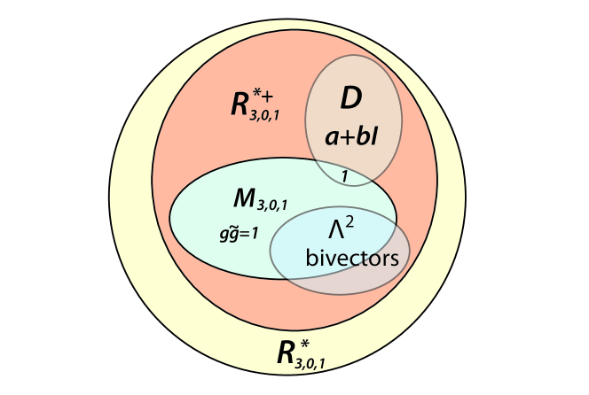
Figure 13: Venn diagram showing the inclusion relationships of the algebra $\mathbf{P}(\mathbb{R}^{*}_{3,0,1})$, its even subalgebra $\mathbf{P}(\mathbb{R}^{*+}_{3,0,1})$, the dual numbers $\mathbb{D}$, the motor group $\mathfrak{M}_{3,0,1}$, and the bivectors $\bigwedge^{2}$.

Calculating the logarithm of a motor. The logarithm ${\mathbf{\Theta}}$ of a motor $\mathbf{m}$ is an algebra element that satisfies $\mathbf{m}=e^{{\mathbf{\Theta}}}$. We now show how to find such a logarithm. We know the normalized motor $\mathbf{m}$ contains only even-grade parts:

$$\mathbf{m} =\langle\mathbf{m}\rangle_{0}+\langle\mathbf{m}\rangle_{2}+\langle\mathbf{m}\rangle_{4}$$ (4)

$$=s_{1}+{\mathbf{\Theta}}+p_{1}\mathbf{I}$$ (5)

$$=(s_{1}+p_{1}\mathbf{I})+(s_{2}+p_{2}\mathbf{I})\widehat{{\mathbf{\Theta}}}$$ (6)

In the last line we have substituted ${{\mathbf{\Theta}}}=\|{\mathbf{\Theta}}\|\widehat{{\mathbf{\Theta}}}$ (see above Sect. 8.1.3). Comparing coefficients in Eq. 3 and Eq. 6 we see that we have an overdetermined system: from the four quantities $\{s_{1},p_{1},s_{2},p_{2}\}$ we have to deduce the two parameters $\{u,v\}$. This leads to the following values for $u$ and $v$:

$$u:=\tan^{-1}(s_{2},s_{1}),\leavevmode\nobreak\ v:=\cfrac{p_{2}}{s_{1}} \leavevmode\nobreak\ \leavevmode\nobreak\ \leavevmode\nobreak\ \leavevmode\nobreak\ \text{for}\leavevmode\nobreak\ s_{1}\neq 0$$ (7)

$$u:=\tan^{-1}(-p_{1},p_{2}),\leavevmode\nobreak\ v:=\cfrac{-p_{1}}{s_{2}}$$ otherwise (8)

Note that either $s_{1}\neq 0$ or $s_{2}\neq 0$ since otherwise $\mathbf{m}^{2}=0$. Then

$$e^{(u+v\mathbf{I})\widehat{{\mathbf{\Theta}}}}=\mathbf{m}$$

$(u+v\mathbf{I})\widehat{{\mathbf{\Theta}}}$ is the logarithm of $\bf{m}$. It is unique except for adding multiples of $2\pi$ to $u$. The pitch of the screw motion is given by the proportion $v:u$. The logarithm shows that $\mathbf{m}$ can be decomposed as

$$e^{u\widehat{{\mathbf{\Theta}}}}e^{v\widehat{{\mathbf{\Theta}}}^{\perp}}$$

that is, the composition (in either order) of a rotation through angle $2u$ around the axis $\widehat{{\mathbf{\Theta}}}$ and a translation of distance $2v$ around the polar axis $\widehat{{\mathbf{\Theta}}}^{\perp}$.

Axis of bivector or axis of screw motion? These formulas make clear that the two uses of axis that we have encountered are actually the same. The axis pair of a screw motion (considered as the unique pair of invariant lines) is the axis pair of its bivector part.

Connection to Lie groups and Lie algebras. By establishing the logarithm function (unique up to multiples of $2\pi$), we have established that the exponential map $\exp:\bigwedge^{2}\rightarrow\mathfrak{M}_{3,0,1}$ is invertible. Hence we are justified in identifying $\mathfrak{M}_{3,0,1}$ as a Lie group and $\bigwedge^{2}$ as its Lie algebra, and can apply the well-developed Lie theory to this aspect of PGA.

This concludes our introductory treatment of the geometric product in $\mathbf{P}(\mathbb{R}^{*}_{3,0,1})$. We turn now to its formulation of rigid body mechanics, whose essential features were already known to Plücker and Klein in terms of 3D line geometry ([Zie85]).

8.2 Kinematics and Mechanics in $\mathbf{P}(\mathbb{R}^{*}_{3,0,1})$

Here we give a very abbreviated overview of the treatment of kinematics and rigid body mechanics in PGA in the form of a bullet list.

1. Kinematics deal with continuous motions in $\mathbf{E}^{3}$, that is, paths in $\mathfrak{M}_{3,0,1}$. Let $\mathbf{g}(t)$ be such a path describing the motion of a rigid body.

2. There are two coordinate systems for a body moving with $\mathbf{g}$: body and space. An entity $\mathbf{x}$ can be represented in either: $\mathbf{X}_{c}$/$\mathbf{X}_{s}$ represents body/space frame.

3. The velocity in the body ${\mathbf{\Omega}}_{c}:=\widetilde{\mathbf{g}}\dot{\mathbf{g}}$; in space, ${\mathbf{\Omega}}_{s}:=\dot{\mathbf{g}}\widetilde{\mathbf{g}}$. ${\mathbf{\Omega}}_{c}$ and ${\mathbf{\Omega}}_{s}$ are bivectors.

4. A, the inertia tensor of the body, is a 6D symmetric bilinear form

   $$J^{-1}(\text{{A}}({\mathbf{\Omega}}_{c}))={\mathbf{\Pi}}_{c}\leavevmode\nobreak\ \leavevmode\nobreak\ \leavevmode\nobreak\ \text{and}\leavevmode\nobreak\ \leavevmode\nobreak\ \leavevmode\nobreak\ {\mathbf{\Omega}}_{c}=\text{{A}}^{-1}(J({\mathbf{\Pi}}_{c}))$$

   where ${\mathbf{\Pi}}_{c}$ is the momentum in the body and $J$ is Poincaré duality map.

5. The kinetic energy $E$ satisfies $E={\mathbf{\Omega}}_{c}\wedge{\mathbf{\Pi}}_{c}$.

6. Let $\mathbf{\Phi}_{c}$ represent the external forces in body frame. Then $\dot{E}=-2\mathbf{\Phi}_{c}\vee{\mathbf{\Omega}}_{c}$.

7. The work done can be computed as

   $$w(t)=E(t)-E(0)=\int_{0}^{t}{\dot{E}ds}=-2\int_{0}^{t}{\mathbf{\Phi}_{c}\vee{\mathbf{\Omega}}_{c}ds}$$

8. The Euler equations of motion for the of the motion free top one obtains the following Euler equations of motion:

   $$\dot{\mathbf{g}} =\mathbf{g}{\mathbf{\Omega}}_{c}$$ (9)

   $$\dot{{\mathbf{\Omega}}}_{c} =\mathbf{A}^{-1}(\mathbf{\Phi}_{c}+2\mathbf{A}({\mathbf{\Omega}}_{c})\times{\mathbf{\Omega}}_{c})$$ (10)

Theoretical discussion. The traditional separation of both velocities and momenta into linear and angular parts disappears completely in PGA, further evidence of its polymorphicity. The special, awkward role assigned to the coordinate origin in the calculation of angular quantities (moment of a force, etc.) along with many mysterious cross-products likewise disappear.

What remains are unified velocity and momentum bivectors that represent geometric entities with intuitive significance. We have already above seen how the velocity can be decomposed into an axis pair that completely describes the instantaneous motion at time $t$. Similar remarks are valid also for momentum and force bivectors. We focus on forces now but everything we say also applies to momenta. The simple bivector representing a simple force is the line carrying the force; the weight of the bivector is the intensity of the force. A force couple is a simple force carried by an ideal line (like a translation is a “rotation” around an ideal line). Systems of forces that do not reduce to a simple bivector can be decomposed into an axis pair exactly as the velocity bivector above, combining a simple force with an orthogonal force couple. This axis pair has to be interpreted however in a dynamical, not kinematical, setting. Further discussion lies outside the scope of these notes.

Practical discussion. The above Euler equations equations behave particularly well numerically: the solution space has 12 dimensions (the isometry group is 6D and the momentum space (bivectors) also) while the integration space has 14 dimensions ($\mathbf{P}(\mathbb{R}^{*+}_{3,0,1})$ has dimension 8 and the space of bivectors has 6). Normalizing the computed motor $\mathbf{g}$ brings one directly back to the solution space. In traditional matrix approaches as well as the CGA approach ([LLD11]), the co-dimension of the solution space within the integration space is much higher and leads typically to the use Lagrange multipliers or similar methods to maintain accuracy. This advantage over VLAAG and CGA is typical of the PGA approach for many related computing challenges.

See [Gun11b] or [Gun11a], Ch. 9, for details on rigid body mechanics in $\mathbf{P}(\mathbb{R}^{*}_{3,0,1})$. For a compact, playable PGA implementation see [Ken17a].

9 Automatic differentiation

[HS87] introduces the term “geometric calculus” for the application of calculus to geometric algebras, and shows that it offers an attractive unifying framework in which many diverse results of calculus and differential geometry can be integrated. While a treatment of geometric calculus lies outside the scope of these notes, we want to present a related result to give a flavor of what is possible in this direction.

We have already met above, in Sect. 8.1.3, the 2-dimensional sub-algebra of $\mathbf{P}(\mathbb{R}^{*}_{n,0,1})$ consisting of scalars and pseudoscalars known as the dual numbers. It can be abstractly characterized by the fact that $1^{2}=1$ while $\mathbf{I}^{2}=0$. Already Eduard Study, the inventor of dual numbers, realized that they can be used to do automatic differentiation ([Stu03], Part II, §23). A modern reference describes how [Wik]:

Forward mode automatic differentiation is accomplished by augmenting the algebra of real numbers and obtaining a new arithmetic. An additional component is added to every number which will represent the derivative of a function at the number, and all arithmetic operators are extended for the augmented algebra. The augmented algebra is the algebra of dual numbers.

This extension can be obtained by beginning with the monomials. Given $p_{k}(x)=x^{k}$, define

$$p_{k}(x+y\mathbf{I}):=(x+y\mathbf{I})^{k}=x^{k}+nx^{n-1}y\mathbf{I}$$

All higher terms disappear since $\mathbf{I}^{2}=0$. Setting $y=1$ we obtain

$${p}_{k}(x+\mathbf{I})=p_{k}(x)+\dot{p}_{k}(x)\mathbf{I}$$

That is, the scalar part is the original polynomial and the pseudoscalar, or dual, part is its derivative. In general if $u$ is a function $u(x)$ with derivative $\dot{u}$, then

$$p_{k}(u+\dot{u}\mathbf{I})=p_{k}(u)+\dot{p}_{k}(u)\mathbf{I}$$

Thus, the coefficient of $\mathbf{I}$ tracks the derivative of $p_{k}$. Extend these definitions to polynomials by additivity in the obvious way. Since the polynomials are dense in the analytic functions, the same “dualization” can be extended to them and one obtains in this way robust, exact automatic differentiation. One can also handle multivariable functions of $n$ variables, using the $(n)$ ideal $n-$vectors $E_{i}$ for $i>0$ (representing the ideal directions of euclidean $n$-space) as the nilpotent elements instead of $\mathbf{I}$. For a live JavaScript demo see [Ken17a].

10 Implementation issues

Our description would be incomplete without discussion of the practical issues of implementation. This has been the focus of much work and there exists a well-developed theory and practice for general geometric algebra implementations to maintain performance parity with traditional approaches. See [Hil13]. PGA presents no special challenges in this regard; in fact, it demonstrates clear advantages over other geometric algebra approaches to euclidean geometry in this regard ([Gun17b]). For a full implementation of PGA in JavaScript ES6 see Steven De Keninck’s ganja.js project on GitHub [Ken17b] and the interactive example set at [Ken17a].

PGA	VLAAG
Unified representation for points, lines, and planes based on a graded exterior algebra; all are “equal citizens” in the algebra.	The basic primitives are points and vectors and all other primitives are built up from these. For example, lines in 3D sometimes parametric, sometimes w/ Plücker coordinates.
Projective exterior algebra provides robust meet and join operators that deal correctly with parallel entities.	Meet and join operators only possible when homogeneous coordinates are used, even then tend to be ad hoc since points have distinguished role and ideal elements rarely integrated.
Unified, high-level treatment of euclidean (“finite”) and ideal (“infinite”) elements of all dimensions. Unifies e.g. rotations and translations, simple forces and force couples.	Points (euclidean) and vectors (ideal) have their own rules, user must keep track of which is which; no higher-dimensional analogues for lines and planes.
Unified representation of isometries based on sandwich operators which act uniformly on points, lines, and planes.	Matrix representation for isometries has different forms for points, lines, and planes.
Same representation for operator and operand: $\mathbf{m}$ is the plane as well as the reflection in the plane.	Matrix representation for reflection in $\mathbf{m}$ is different from the vector representing the plane.
Compact, universal expressive formulas and constructions based on geometric product (see Tables 3, 4, and 5) valid for wide range of argument types and dimensions.	Formulas and constructions are ad hoc, complicated, many special cases, separate formulas for points/lines/planes, for example, compare [Gla90].
Well-developed theory of implementation optimizations to maintain performance parity.	Highly-optimized libraries, direct mapping to current GPU design.
Automatic differentiation of real-valued functions using dual numbers.	Numerical differentiation

Table 6: A comparison of PGA with the standard VLAAG approach.

11 Comparison

Table 6 encapsulates the foregoing results in a feature-by-feature comparison with the standard (VLAAG) approach. It establishes that PGA fulfills all the features on our wish-list in Sec. 2, while the standard approach offers almost none of them. (For a proof that PGA is coordinate-free, see the Appendix in [Gun17a].)

11.1 Conceptual differences

How can we characterize conceptually the difference of the two approaches leading to such divergent results?

• First and foremost: VLAAG is point-centric: other geometric primitives of VLAAG such as lines and planes are built up out of points and vectors. PGA on the other hand is primitive-neutral: the exterior algebra(s) at its base provide native support for the subspace lattice of points, lines and planes (with respect to both join and meet operators).

• Secondly, the projective basis of PGA allows it to deal with points and vectors in a unified way: vectors are just ideal points, and in general, the ideal elements play a crucial role in PGA to integrate parallelism, which typically has to be treated separately in VLAAG. The existence of the ideal norm in PGA goes beyond the purely projective treatment of incidence, producing polymorphic metric formulas that, for example, correctly handle two intersecting lines whether they intersect or are parallel (see above Sect. 7.2).

• The representation of isometries using sandwich operators generated by reflections in planes (or lines in 2D) can be understood as a special case of this “compact polymorphicity”: the sandwich operator $\mathbf{g}\mathbf{X}\tilde{\mathbf{g}}$ works no matter what $X$ is, the same representation works whether it appears as operator or as operand, and rotations and translations are handled in the same way.

11.2 The expressiveness of PGA

All these conceptual differences contribute to the astounding richness of the PGA syntax in comparison to VLAAG, a richness exemplified in the formulas of tables 3, 4, and 5. Each of the conceptual differences in the above list can be thought of as a set of distinctions that are embedded in a unified form within the PGA syntax: points/lines/planes, euclidean/ideal, operator/operand, etc. This leads to having many more basic expressions for modeling geometry than in VLAAG, and they all combine meaningfully with each other. To the best of our knowledge these formula collections establish PGA as the “world champion” among all existing frameworks for euclidean geometry with respect to compactness, completeness, and polymorphicity. Compare [Gla90] for selected VLAAG analogs. Readers who know of a competitive formula collection are urged to drop the author an email with a pointer to it. We also expect that there are more formulas waiting to be discovered (after all, here we’ve only considered the 2-way products and a small subset of the 3-way products).

Non-euclidean metrics. The expressiveness of PGA takes on a wider dimension when we recall that PGA is actually a family of geometric algebras. We have focused attention here on euclidean PGA. The other members of the family model non-euclidean spaces, notably, spherical and hyperbolic space. Simply by specifying a different value for $\mathbf{e}_{0}^{2}$, these other PGA’s can also be accessed. Many of the formulas and constructions included in these notes can be applied unchanged to these other metric spaces (for example, the treatment of rigid body mechanics included above is metric-neutral in this sense, as are many of the constructions in the tables) or with minor and instructive differences with respect to EPGA. The example of spherical geometry in Sect. 6.3 illustrates the power of this approach. [Gun11a] develops all its PGA results in the setting of all three classical metrics.

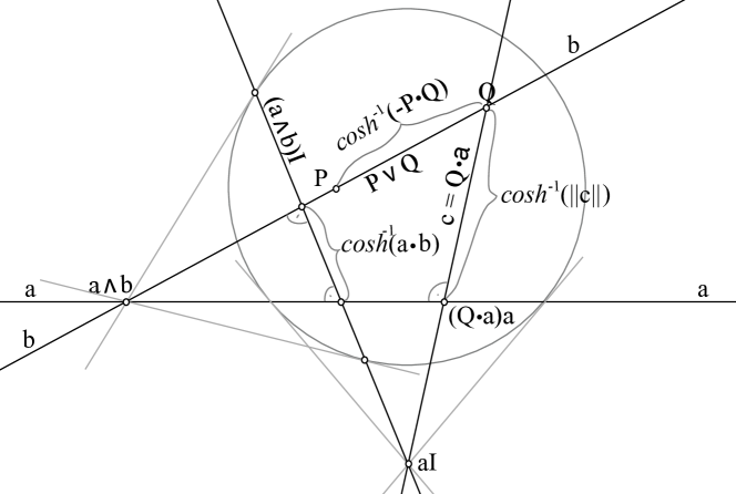
Figure 14: Doing geometry in the hyperbolic plane using the PGA $\mathbf{P}(\mathbb{R}^{*}_{2,1,0})$.

11.3 The universality of PGA

The previous section highlighted the structural advantages enjoyed by PGA over VLAAG. We strengthen this argument in this section by showing that alternate approaches to euclidean geometry are largely present already in PGA as parts of the whole.

11.3.1 Vector algebra

The previous section has already suggested that VLAAG can be seen less as a direct competitor to PGA than as a restricted subset. Indeed, restricting attention to the vector space of $n$-vectors (sometimes written $\bigwedge^{n}$) in PGA essentially yields standard vector algebra. Define the “points” to be euclidean $n$-vectors ($\mathbf{P}^{2}\neq 0$) and “vectors” to be ideal $n$-vectors ($\mathbf{P}^{2}=0$). All the rules of vector algebra can be then derived using the vector space structure of $\bigwedge^{n}$ equipped with the standard and ideal PGA norms (assuming normalized arguments as usual). The absence of the geometric product in this context makes clear why VLAAG is so much “smaller” than PGA.

Unified $\mathbb{R}^{n}$ and $\mathbf{E}^{n}$. This embedding of vector algebra in PGA also comes with a nice geometric intuition absent in traditional vector algebra: the vectors make up the ideal plane bounding the euclidean space of points, i. e., points and vectors make up a connected, unified space (topologically equivalent to projective space $\mathbb{R}{P^{n}}$). Furthermore, intuitions developed in vector algebra such as “Adding a vector to a point translates the point.” have natural extensions in PGA: adding an ideal line (plane) to a euclidean line (plane) translates the line (plane) parallel to itself. Such patterns are legion.

11.3.2 Linear algebra and analytic geometry

Note that PGA is fully compatible with the use of linear algebra. A linear map on the 1-vectors has induces linear maps on all grades of the algebra that can be automatically computed and applied. The big difference to VLAAG is that linear algebra no longer is needed to implement euclidean motions – a role for which it is not particularly well-suited. We envision the development of an analytic geometry based on the full extent of PGA, not just on the small subset present in VLAAG, and would have at its disposal the geometric calculus sketched in Sect. 9. Traditional analytic geometry would make up a small subset of this extended analytic geometry, like vector algebra makes up a small part of PGA proper.

11.3.3 Exterior algebra

The underlying graded algebra structure of PGA can be thought of as being inherited from the exterior algebra. The wedge product is just the highest grade part of the geometric product, and implements the meet operator in PGA. The join operator is available from the dual exterior algebra via Poincaré duality (see Sect. 5.10).

11.3.4 Quaternions and dual quaternions

Many aspects of PGA are present in embryonic form in quaternions and dual quaternions, but they only find their full expression and utility when embedded in the full algebra PGA. Indeed, the quaternion and dual quaternion algebras are isomorphically embedded in the even sub-algebra $\mathbf{P}(\mathbb{R}^{*+}_{n,0,1})$ for $n\geq 3$.

Integrated with points and planes. The advantage of the embedding in PGA are considerable. The full algebraic structure of PGA provides a much richer environment than these quaternion algebras alone. At the most basic level, quaternion and dual quaternion sandwich operators only model direct isometries; the embedding in PGA reveals how they arise naturally as even compositions of the reflections provided by sandwiches with 1-vectors. Furthermore, few of the formulas in Tables 3, 4, and 5 are available in the quaternion algebras alone since the latter only have natural representations for primitives of even grade (essentially bivectors for $n=2$ and $n=3$). For example, in PGA, you can apply all sandwiches to geometric primitives of any grade. In contrast, one of the “mysteries” of contemporary dual quaternion usage is that there are separate ad hoc representations for points, lines, and planes and slightly different forms of the sandwich operator for each in order to be able to apply euclidean direct isometries. These eccentricities disappear when, as in PGA, there are native representations for points and planes, see [Gun17b], §3.8.1.

Demystifying $\epsilon$ and the legacy of William Clifford. The PGA embedding clears up other otherwise mysterious aspects of current dual quaternion practice. Consider the dual unit $\epsilon$ satisfying $\epsilon^{2}=0$. In the embedding map, it maps to the pseudoscalar $\mathbf{I}$ of the algebra (for details see [Gun11a], §7.6), perhaps tarnishing the mystique but replacing it with a deeper understanding of the genesis of the dual quaternions. It is also here worth noting that William Clifford invented both dual quaternions (or biquaternions as he called them) and geometric algebra. That he did not also discover their happy reunion in EPGA is most likely due to his early death at age 34. At the time of his death neither the dual construction of the exterior algebra nor the degenerate metric (both necessary ingredients of eucidean PGA) had been introduced to the study of geometric algebras.

12 Conclusion

We have established that euclidean PGA fulfills the developers’ wish list with which we began these notes, offering numerous advantages over the existing VLAAG approach. The natural next question for interested developers is, what is involved in migrating to PGA from one of the alternatives discussed above? In fact, the use of homogeneous coordinates and the inclusion of quaternions, dual quaternions, and exterior algebra in PGA means that many practitioners already familiar with these tools can expect a gentle learning curve. Furthermore, the availability of a JavaScript implementation on GitHub ([Ken17b]) and the existence of platforms such as Observable notebooks [Bos18] means that interested users, equipped with the attached “cheat sheets” for 2D and 3D PGA, can quickly get to work to prototype and share their applications. Readers who would like to deepen their understanding of the underlying mathematics are referred to the literature [Gun11c], [Gun11a], [Gun17b], [Gun17a]. We intend also to establish an on-line presence for PGA that will facilitate the exchange of information among the community of users, that we will announce at the course meeting in Los Angeles in July 2019.

References

- [Bos18] Mike Bostock. Observable notebooks: a reactive JavaScript environment, 2018. https://observablehq.com.
- [Cli73] William Clifford. A preliminary sketch of biquaternions. Proc. London Math. Soc., 4:381–395, 1873.
- [Cli78] William Clifford. Applications of Grassmann’s extensive algebra. American Journal of Mathematics, 1(4):pp. 350–358, 1878.
- [Gla90] Andrew S. Glassner. Useful 3d geometry. In Andrew S. Glassner, editor, Graphics Gems, pages 297–300. Academic Press, 1990.
- [Gra44] Hermann Grassmann. Ausdehnungslehre. Otto Wigand, Leipzig, 1844.
- [Gun11a] Charles Gunn. Geometry, Kinematics, and Rigid Body Mechanics in Cayley-Klein Geometries. PhD thesis, Technical University Berlin, 2011. http://opus.kobv.de/tuberlin/volltexte/2011/3322.
- [Gun11b] Charles Gunn. On the homogeneous model of euclidean geometry. In Leo Dorst and Joan Lasenby, editors, A Guide to Geometric Algebra in Practice, chapter 15, pages 297–327. Springer, 2011.
- [Gun11c] Charles Gunn. On the homogeneous model of euclidean geometry: Extended version. http://arxiv.org/abs/1101.4542, 2011.
- [Gun17a] Charles Gunn. Doing euclidean plane geometry using projective geometric algebra. Advances in Applied Clifford Algebras, 27(2):1203–1232, 2017. http://arxiv.org/abs/1501.06511.
- [Gun17b] Charles Gunn. Geometric algebras for euclidean geometry. Advances in Applied Clifford Algebras, 27(1):185–208, 2017. http://arxiv.org/abs/1411.6502.
- [Hil13] Dieter Hildebrand. Fundamentals of Geometric Algebra Computing. Springer, 2013.
- [HS87] David Hestenes and Garret Sobczyk. Clifford Algebra to Geometric Calculus. Fundamental Theories of Physics. Reidel, Dordrecht, 1987.
- [Ken17a] Steven De Keninck. Ganja coffeeshop, 2017. https://enkimute.github.io/ganja.js/examples.
- [Ken17b] Steven De Keninck. Ganja: Geometric algebra for javascript, 2017. https://github.com/enkimute/ganja.js.
- [LLD11] Anthony Lasenby, Robert Lasenby, and Chris Doran. Rigid body dynamics and conformal geometric algebra. In Leo Dorst and Joan Lasenby, editors, Guide to Geometric Algebra in Practice, chapter 1, pages 3–25. Springer, 2011.
- [Möb37] A. F. Möbius. Lehrbuch der Statik. Göschen, Leibzig, 1837.
- [Stu91] Eduard Study. Von den Bewegungen und Umlegungen. Mathematische Annalen, 39:441–566, 1891.
- [Stu03] Eduard Study. Geometrie der Dynamen. Tuebner, Leibzig, 1903.
- [Wik] Wikipedia. https://en.wikipedia.org/wiki/Automatic_differentiation.
- [Zie85] Renatus Ziegler. Die Geschichte Der Geometrischen Mechanik im 19. Jahrhundert. Franz Steiner Verlag, Stuttgart, 1985.