Relaxation time of a polymer glass stretched at very large strains

Abstract

The polymer relaxation dynamic of a sample, stretched up to the stress hardening regime, is measured, at room temperature, as a function of the strain $\lambda$ for a wide range of the strain rate $\dot{\gamma}$, by an original dielectric spectroscopy set up. The mechanical stress modifies the shape of the dielectric spectra mainly because it affects the dominant polymer relaxation time $\tau$, which depends on $\lambda$ and is a decreasing function of $\dot{\gamma}$. The fastest dynamics is not reached at yield but in the softening regime. The dynamics slows down during the hardening, with a progressive increase of $\tau$. A small influence of $\dot{\gamma}$ and $\lambda$ on the relative dielectric strength cannot be excluded.

Mechanical and dynamical properties of polymers are intensively studied, due to their fundamental and technological importance Ferry (1980). When strained at a given strain rate, beyond the elastic regime in which the stress is proportional to strain, glassy polymers exhibit a maximum in the stress-strain curves (yield point) at a strain of a few percents Nielsen and Landel (1994) and the deformation becomes irreversible (see Fig.1). At larger strains, depending on the history of the sample Meijer and Govaert (2003), the stress drops (strain-softening regime) before reaching a plateau corresponding to plastic flow. Strain-hardening may then occur at even larger strains, depending on the molecular weight and on the cross-linking of the polymer Meijer and Govaert (2005). The key new insights obtained either by numerical simulations Hoy and Robbins (2006); Hoy and O’Hern (2010); Hoy (2011) or experiments Van Melick et al. (2003); Govaert et al. (2008); Senden et al. (2010); Jatin et al. (2014) are that strain hardening appears to be controlled by the same mechanisms that control plastic flow Chui and Boyce (1999); Hasan and Boyce (1993); Hoy and Robbins (2009); Ge and Robbins (2010). However the microscopic mechanisms leading to such a mechanical behavior are not fully understood Kramer (2005); Hoy (2016). For example it is unclear to what extent the relaxation dynamics in polymer glasses is modified when the sample is stretched into the plastic region (see for example refs.Nicolas et al. (2018); Conca et al. (2017); Jaiswal et al. (2016); Roth (2016)).

The purpose of this letter is to bring new insight into this problem by presenting the results of experiments in which we performed dielectric spectroscopy of polymer samples stretched till the strain hardening regime. Dielectric spectroscopy, allows the investigation of the dynamics of relaxation processes by means of the polarization of molecular dipoles. It is directly sensitive to polymer mobility and probes directly the segmental motion. It can be used to quantify the mobile fraction of polymers. Measuring the dielectric response of polymers in situ had been pioneered by Venkataswamy et al. Venkatasway et al. (1982). It is complementary to other techniques, such as Nuclear Magnetic Resonance Loo et al. (2000) and the diffusion of probe molecules Ediger (2000); Bending et al. (2014); Hebert et al. (2015), used to study the molecular dynamics of polymers under stress. The dielectric spectroscopy has already been used in combination with mechanical deformation to study the dynamics in the amorphous phase of polymer under stress Kalfus et al. (2012); Perez-Aparicio et al. (2016).

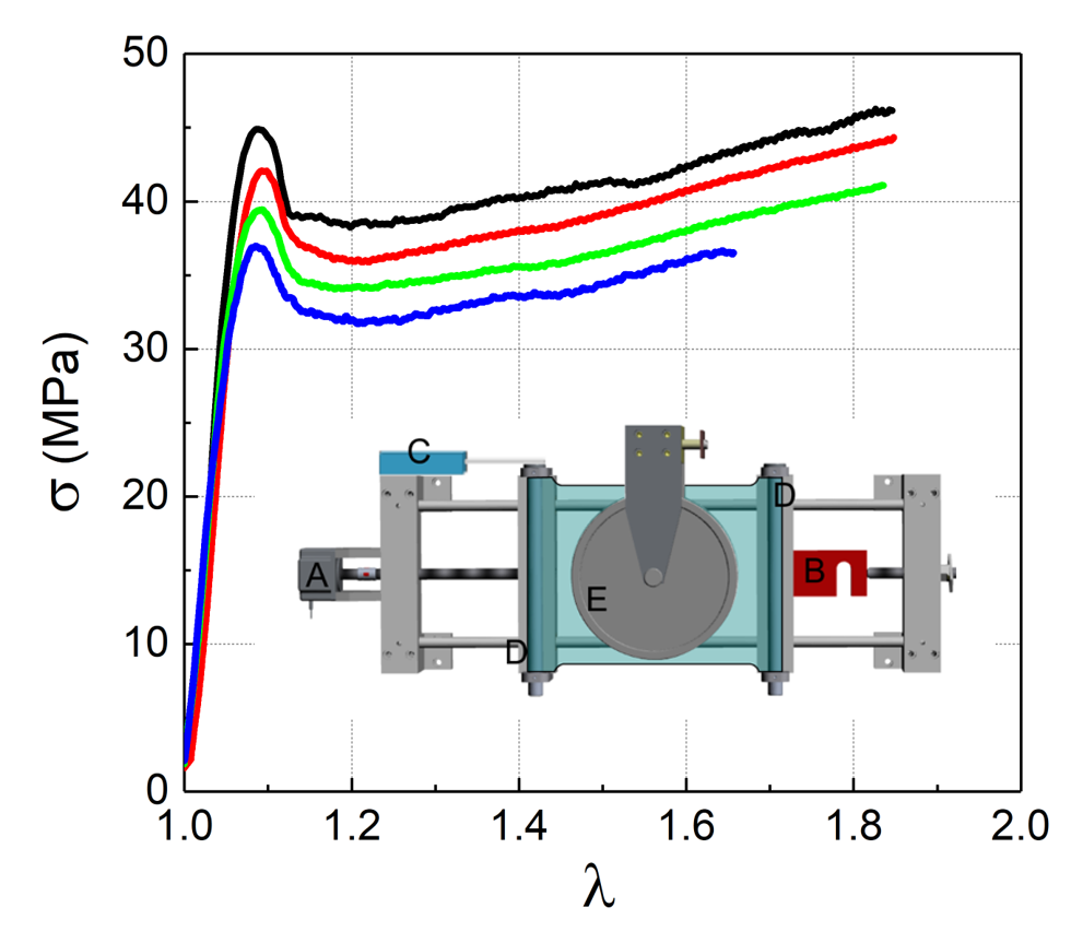
Figure 1: Stress evolution over a wide range of $\lambda$ at several constant strain rates : $2.5\times 10^{-3}s^{-1}$ (black), $2.5\times 10^{-4}s^{-1}$ (red), $2.5\times 10^{-5}s^{-1}$ (green) and $2.5\times 10^{-6}s^{-1}$ (blue). Several identical specimens have been measured for each strain rate. Inset: tensile machine for dielectric measurements under stress : motor (A), load cell (B), linear transducer (C), sample fastening cylinders with the stretched polymer film (D) and electrodes (E) connected to the dielectric spectrometer (not sketched).

The results of these experiments were limited to the yield point whereas the experimental studies of the microscopic behavior and processes during strain hardening are more scarce.

In this letter we present the results obtained by our original experimental apparatus which can measure with high accuracy the evolution of the Dielectric Spectrum(DS) of a sample stretched, till the strain hardening regime, at different strain rates. Thus we can precisely compare the $\text{DS}_{s}$obtained as a function of stress at room temperature with those (named $\text{DS}_{T}$) obtained as a function of temperature in an unstressed sample. This comparison allows us to extract useful informations on the relaxation dynamics under stress at various strain rates. Our experimental results bring new important informations because they clearly show an acceleration of the dynamics which reaches a maximum in the softening regions. Instead the molecular mobility slows down again during the strain hardening regimes.

Our experimental setup is composed by a home-made dielectric spectrometer coupled with a tensile machine for uniaxial stretching of films Pérez-Aparicio et al. (2015); Perez-Aparicio et al. (2016). The scheme of the experimental setup is presented in the inset of Fig. 1. More details are given in Annex I.1.

The dielectric measurements are performed by confining the polymer film between two disc-shaped electrodes of 10 cm diameter. The good contact between the electrodes and the sample, during the whole experiment, is assured by an aqueous gel, which has very low electrical resistivity compared to the sample. We checked that the gel does not perturb the sample response because water absorption in our samples is only 0.2% and by comparing the response in the presence of the aqueous gel and in the presence of mineral oil Pérez-Aparicio et al. (2015).

Dielectric spectroscopy allows the investigation of the dielectric response of a material as a function of the angular frequency $\omega$. It is expressed by the complex dielectric permittivity or dielectric constant: $\varepsilon(\omega)=\varepsilon^{\prime}(\omega)-i\varepsilon^{\prime\prime}(\omega)$, with $\varepsilon^{\prime}(\omega)$ the real component of the dielectric constant which is related to the electric energy stored by the sample, and $\varepsilon^{\prime\prime}(\omega)$ the imaginary component which indicates the energy losses. The loss tangent is $\text{tn}\delta(\omega)=\tan\delta(\omega)=\varepsilon^{\prime\prime}(\omega)/\varepsilon^{\prime}(\omega)$, where $\delta$ is the phase shift between the electric field applied for measuring $\varepsilon$ and the measured dielectric polarization.

We investigated an extruded film MAKROPOL^® DE 1-1 000000 (from BAYER) based on Makrolon^® polycarbonate (PC) with a $T_{g}$ of about 150 ^∘C. The sample sheets had a thickness of 125 $\mu$m. The tensile experiments are performed at $T=25^{\circ}$C much below $T_{g}$. We fixed four different strain rates: $2.5\times 10^{-3}$ s^-1, $2.5\times 10^{-4}$ s^-1, $2.5\times 10^{-5}$ s^-1 and $2.5\times 10^{-6}$ s^-1. Typical strain curves at the different strain rates are plotted in Fig.1. Initially, the stress increases almost linearly up to its maximum (yield stress) which is reached at $\lambda\simeq 1.08$. The stress decreases after the yield strain softening regime for $1.09<\lambda<1.2$. For $\lambda>1.2$, the material is inside the strain hardening regime, where the force increases up to the film crack.

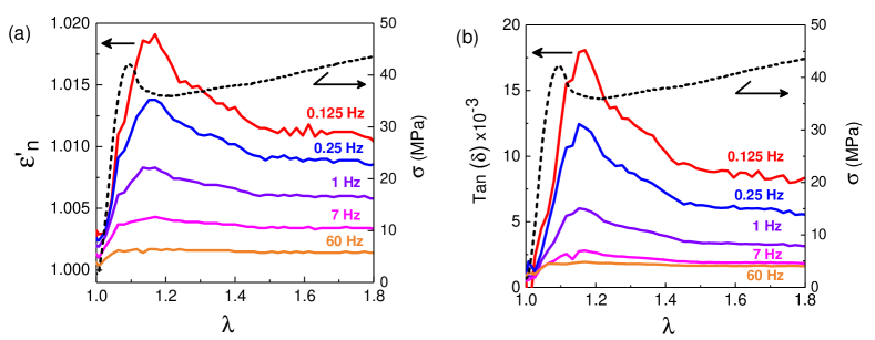
Figure 2: Dependence on $\lambda$ of ${\varepsilon^{\prime}_{n}}$ (a) and $\text{tn}\delta$ (b) measured at several frequencies during the stretching experiment at $\dot{\gamma}=2.5\times 10^{-4}s^{-1}$. In both panels the solid lines (left hand ordinate) represent ${\varepsilon^{\prime}_{n}}$(a) and $\text{tn}\delta$(b) as a function of $\lambda$, whereas the dashed line (right hand ordinate) show the corresponding evolution of the stress, which reveals that the low frequency components of $\text{DS}_{s}$have a maximum in the softening regime of the polymer film.

In this article we focus on the measurement at $\lambda>1.09$ being the results at $\lambda\leq 1.08$ already discussed in Perez-Aparicio et al. (2016). For each value of the strain rate the measurement of the dielectric and mechanical properties have been repeated on at least 3 samples, in order to check the reproducibility of the results. The maximum fluctuations of the results observed in different samples is at most $11\%$. In order to compensate for the change of the thickness of the sample we study ${\varepsilon^{\prime}_{n}}(f)=\varepsilon^{\prime}(f,\lambda)/\varepsilon^{\prime}(400Hz,\lambda)$ because above 400Hz the only effect of the applied stress on the dielectric measurement is related to the change of the sample thickness induced by the large applied stress. The quality of this compensation can be checked looking at Figs.2 where we plot ${\varepsilon^{\prime}_{n}}(f,\lambda)$ and $\text{tn}\delta(f,\lambda)$ measured at various frequencies as a function of $\lambda$. We clearly see that the effect of the stretching on the DS decreases a lot by increasing the measuring frequency and it almost disappears at $60$Hz. This means that ${\varepsilon^{\prime}_{n}}$ cancels the dependence of the sample thickness $d(\lambda)$ and correctly estimates the variation of $\varepsilon$ induced by the strain. This figure also shows that both ${\varepsilon^{\prime}_{n}}$ and $\text{tn}\delta$ reach the maximum in the softening regime then they decrease and remain constant in the hardening regimes. Fig.3 shows that the effect of the strain on $\varepsilon$ increases with $\dot{\gamma}$ as already shown in ref.Perez-Aparicio et al. (2016).

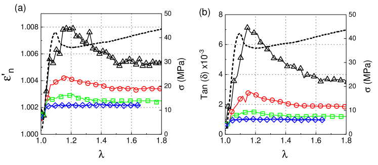
Figure 3: Normalized real part ${\varepsilon^{\prime}_{n}}$ (a) and $\text{tn}\delta$ (b) as a function of $\lambda$ measured at $7$Hz for different strain rates : $2.5\times 10^{-3}s^{-1}$ (black triangles), $2.5\times 10^{-4}s^{-1}$ (red circles), $2.5\times 10^{-5}s^{-1}$ (green squares) and $2.5\times 10^{-6}s^{-1}$ (blue diamonds).

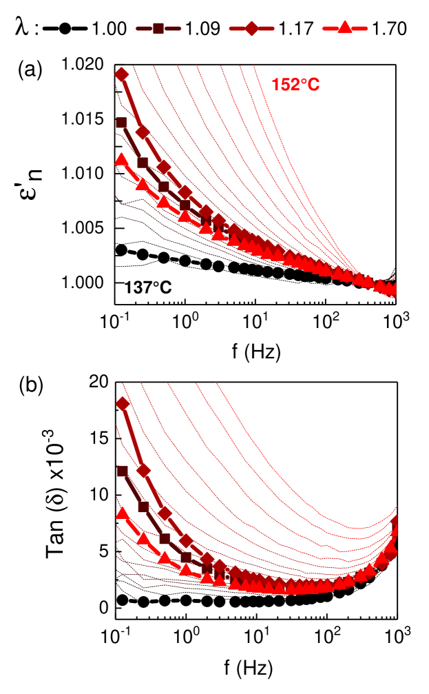
Figure 4: The normalized real part ${\varepsilon^{\prime}_{n}}$ (a) and $\text{tn}\delta$ (b) as a function of frequency measured, at $T=25^{\circ}$C, during a stretching experiment at $2.5\times 10^{-4}s^{-1}$ at different values of the strain : $\lambda=1.00$ (equilibrium), $\lambda=1.08$ (plastic yield), $\lambda=1.17$ (softening regime) and $\lambda=1.70$ (hardening regime). In the background, continuous orange lines represent ${\varepsilon^{\prime}_{n}}$ (a) and $\text{tn}\delta$ (b) measured at $\lambda=1$ in the temperature range between $137^{\circ}C$, (bottom orange curve) and $152^{\circ}C$ (top orange curve) at $1^{\circ}C$ increment Perez-Aparicio et al. (2016).

It is useful to study the evolution of the whole $\text{DS}_{s}$measured at $\dot{\gamma}=2.5\times 10^{-4}s^{-1}$ for which the effect of the strain on $\varepsilon$ is very pronounced (see Fig.2) and at the same time the measure lasts enough time to have a good low frequency resolution of the DS. Figures 4 show ${\varepsilon^{\prime}_{n}}(f)$ and $\text{tn}\delta(f)$ as a function of frequency measured at various $\lambda$ at $\dot{\gamma}=2.5\times 10^{-4}s^{-1}$. The $\text{DS}_{s}$recorded during the tensile test are compared to the $\text{DS}_{T}$, i.e. the DS measured as a function of temperature in the unstressed sample. This figure summarizes one the most important findings of this investigation, that we will explain. First we notice that the low frequency part of $\text{DS}_{s}$has roughly the same amplitude as $\text{DS}_{T}$measured at temperatures close to $T_{g}$. However the $\text{tn}\delta(f)$ of $\text{DS}_{s}$and of $\text{DS}_{T}$have a very different dependence on $f$ indicating that a simple relationship between $\dot{\gamma}$ and an effective temperature ( presented in several articles Guan et al. (2010); Chen and Schweizer (2011); Hebert et al. (2015); Perez-Aparicio et al. (2016, 2016)) cannot be easily established as we discuss later on. However in Figs.4,2 we notice several other important results. We clearly see that in the stressed sample the maximum amplitude of ${\varepsilon^{\prime}_{n}}(f)$ and $\text{tn}\delta$ at low frequencies is not reached at the yield but in the softening regime at $\lambda=1.17$ and most importantly the amplitude of $\text{DS}_{s}$decreases in the hardening regime at $\lambda=1.70$. This is a new and totally unexpected result, i.e. the effect of the strain on the dielectric constant is not monotonous.

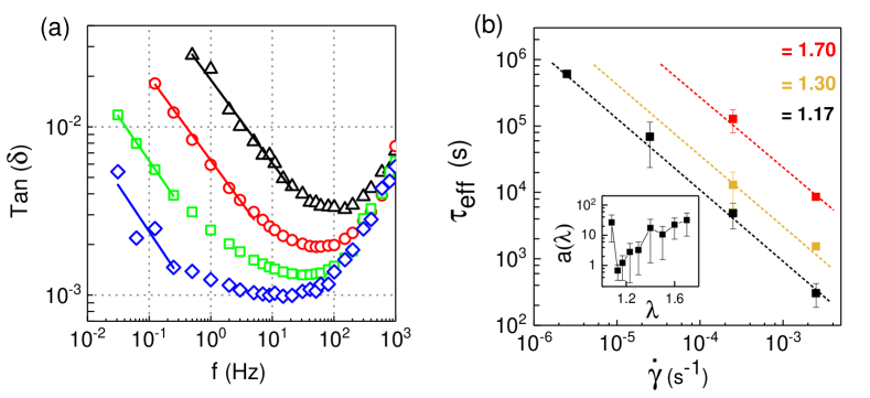
Figure 5: (a) Dependence on frequency of $\text{tn}\delta$, measured in the softening regime $\lambda=1.17$, at different $\dot{\gamma}$: $2.5\times 10^{-3}s^{-1}$ (black triangles), $2.5\times 10^{-4}s^{-1}$ (red circles), $2.5\times 10^{-5}s^{-1}$ (green squares) and $2.5\times 10^{-6}s^{-1}$ (blue diamonds). The low frequency parts of each curve are fitted by a power law (straight lines) $\text{tn}\delta=1/(\omega\tau_{eff})^{\beta}$ The time scale $\tau_{eff}$ depends on $\dot{\gamma}$ but the scaling power $\beta=0.50\pm 0.05$ is found to be constant within experimental errors. (b) The fitted time scale $\tau_{eff}$ as a function of the strain rate $\dot{\gamma}$ measured at several strains: $\lambda=1.17$ (softening regime), $\lambda=1.30$ and $\lambda=1.70$ (hardening regime). The relaxation time follows the law $\tau_{eff}=a(\lambda)/\dot{\gamma}$ (dashed lines) with the coefficient $a(\lambda)$ plotted in the inset.

In order to have a more detailed description of these experimental observations, we study the behavior of $\text{tn}\delta(f,\lambda,\dot{\gamma})$, which is not affected by any geometrical effect. We plot, in Fig.5, $\text{tn}\delta(f)$ versus frequency measured at $\lambda=1.17$ at various $\dot{\gamma}$. We notice that the low frequency parts decrease as a power law which can be fitted with $\text{tn}\delta(\omega)=1/(\omega\tau_{eff})^{\beta}$ where $\tau_{eff}$ and $\beta$ are fitting parameters and $\omega=2\pi f$. We find that $\beta\simeq 0.50\pm 0.05$ is independent of $\dot{\gamma}$ (continuous lines in Fig.5a), with an accuracy of about $10\%$ . The measured time scale $\tau_{eff}$, which is a function of $\dot{\gamma}$ and $\lambda$, is plotted in Fig.5b). Looking at this figure we see that with a very good accuracy $\tau_{eff}=a(\lambda)/\dot{\gamma}$ where $a(\lambda)$ has a minimum at $\lambda\simeq 1.17$ in the stress softening regime.

We can consider the power law behavior of $\text{tn}\delta$ as the high frequency part of the Cole-Cole (Havriliak-Negami) model Havriliak and Negami (1966) for the $\alpha$ peak of the dielectric constant. Indeed, calling $\tau$ the characteristic time of the $\alpha$ peak, at frequencies $\omega>>1/\tau$ the Cole-Cole model takes the form:

$${\varepsilon^{\prime}\over\varepsilon_{\infty}}-1\simeq{(\varepsilon_{o}-\varepsilon_{\infty})\over\varepsilon_{\infty}}\ \ {\cos(\beta\pi/2)\over(\omega\tau)^{\beta}}$$ (1)

and

$$\text{tn}\delta\simeq{(\varepsilon_{o}-\varepsilon_{\infty})\over\varepsilon_{\infty}}\ \ {\sin(\beta\pi/2)\over(\omega\tau)^{\beta}}$$ (2)

where $\varepsilon_{\infty}$ and $\varepsilon_{o}$ are respectively the high and low frequency dielectric constants. In our experiment $\beta\simeq 0.5$ thus the two equations become:

$${\varepsilon^{\prime}\over\varepsilon_{\infty}}-1\simeq{(\varepsilon_{o}-\varepsilon_{\infty})\over\varepsilon_{\infty}}\ \ {1\over(2\omega\tau)^{1/2}},$$ (3)

$$\text{tn}\delta\simeq{(\varepsilon_{o}-\varepsilon_{\infty})\over\varepsilon_{\infty}}\ \ {1\over(2\omega\tau)^{1/2}}.$$ (4)

These two equations show that $\text{tn}\delta\simeq({\varepsilon^{\prime}\over\varepsilon_{\infty}}-1)$ which is rather well verified by the experimental data for all $\lambda$. This indicates that they are a rather good model of the dielectric constant under stress. Using eq.4, we identify the fitting parameter as $\tau_{eff}=2\tau/\Delta^{2}$ where $\Delta={(\varepsilon_{o}-\varepsilon_{\infty})/\varepsilon_{\infty}}$. At this level we cannot distinguish whether the increase of $\varepsilon^{\prime}$ and $\text{tn}\delta$ is induced by a decreasing of $\tau$ or an increase of the relative dielectric strength $\Delta$Frohlich (1958).

We suppose first that the stress has no influence on $\tau$ but only on $\Delta$. Keeping for $\tau$ the value of the unstressed sample we can estimate the value of $\Delta$ under stress from the previous expression $\Delta=\sqrt{2\tau/\tau_{eff}}$. To give a lower bound on the value of $\tau$ at $22^{o}C$ we rely upon the high temperature measurements of the dielectric properties of PC and on the estimation based on the WLF law Huang and McKenna (2001); Perez-Aparicio et al. (2016). For example at $T=130^{o}C$, which is the minimum temperature at which the WLF law for PC can be tested, one finds using WLF $\tau\simeq 10^{7}s$. Thus, as $\tau$ increases by lowering temperature, we simply assume that at $T=22^{o}C$, $\tau>10^{7}s$, which, in addition, is coherent with the fact that our samples are more than one year old Struik (1978).
From the data of fig.5b) we obtain $\tau_{eff}\simeq 1/\dot{\gamma}$ at $\lambda=1.17$. Thus in the hypothesis of constant $\tau$, we find $\Delta>7$ at $\dot{\gamma}=2.5\times 10^{-6}$ and $\Delta>223$ at $\dot{\gamma}=2.5\times 10^{-3}s^{-1}$. This value is 1000 times larger than that of the unstressed sample for which $\Delta\simeq 0.12$. This is nonphysical because $\Delta$ cannot change of such a large amount even at very large strain (see refs.Frohlich (1958); Yee and Smith (1981); Hernández et al. (2013) and appendix I.2). Therefore one has to conclude that, although a small increase of the $\Delta$ cannot be excluded, the observations cannot be explained without a decreasing of $\tau$ with the mechanical stress, i.e. an acceleration of the dynamics, which agrees with other experimental results based on other techniques and other polymers Ediger (2000); Lee et al. (2009); Bending et al. (2014). Using our data we can estimate $\tau\simeq 0.5\Delta^{2}a(\lambda)/\dot{\gamma}$, assuming that $\Delta=0.2$, i.e. keeping fix the value of the unstressed sample. At $\lambda=1.17$ we see that $a(\lambda)\simeq 1$ and using $\dot{\gamma}=2.5\times 10^{-3}$ one finds $\tau=8s$, which implies that one would not observe a clear power law at the highest strain rate because the approximation $\omega>>1/\tau$ will be not fully satisfied for the low frequencies of our frequency range. Therefore at the highest $\dot{\gamma}$, one concludes that $\tau>>8$ s and $\Delta>0.2$. At this point we can safely say that the main effect of the strain is a reduction of $\tau$ of several orders of magnitude although a small influence on $\Delta$ is necessary for the consistency of the observations.

Finally we compare these results with those that one extracts from the values $\text{tn}\delta(f)$ measured in the unstressed sample at different temperatures. In the range $137^{o}C<T<152^{o}C$, where we observe an overlap of $\text{DS}_{s}$and $\text{DS}_{T}$in fig.2 the $\text{tn}\delta(f)$ has a power law dependence on $f$ but the exponent $\beta$ is a function of temperature: specifically $0.25<\beta<0.35$ for $137^{o}C<T<152^{o}C$. The observation that the $\beta$ exponent measured under stress is larger than the one measured in the unstressed sample at temperature close to $T_{g}$, has important consequences. Indeed in the Cole-Cole expression the smallest is the value of the exponent $\beta$ the broadest is the distribution of relaxation times. Thus we conclude that our measurements are compatible with a narrowing of the distribution of relaxation times under stress observed in refs.Lee et al. (2009); Bending et al. (2014) with other techniques in other polymers.

Let us point out that in the frequency window of our measurements there are no other relaxations which may influence the results. The beta relaxation is not affected by the stress because $\text{DS}_{s}$does not change above 400Hz. The gamma relaxation time is at very high frequencies at room temperature (see refYee and Smith (1981)) Structural changes that might also influence the results are absent. Indeed we checked by Differential Scanning Calorimetry (DSC) that polycarbonate does not crystallize under strain in the range considered here. Microscopic damaging may also contribute to the dielectric response. It has been shown that damaging occurs indeed during the strain hardening regime, but the volume fraction corresponding to these damages is very small ($<10^{-4}$ for cellulose acetate Charvet et al. (2019) and for polycarbonate Djukic (2020)) and the corresponding perturbation regarding the interpretation of the results is negligible.

Summarizing, we have studied the $\text{DS}_{s}$of a sample of polycarbonate at room temperature submitted to an applied stress at different strain rates covering three order of magnitude range. In our frequency window we observe that, with respect to the unstressed sample, $\text{tn}\delta$ increases at low frequencies as a function of $\dot{\gamma}$, whereas at high frequencies it remains unchanged. The increase is not monotonous and reaches its maximum in the softening regime. From the data we extract an effective time scale $\tau_{eff}\propto 1/\dot{\gamma}$ which depends on $\lambda$ and reaches its minimum in the softening regime to increase again in the hardening. We have also shown that the distribution of relaxation times is narrower under stress than in the unstressed sample at $T$ close to $T_{g}$. The large variation of $\tau_{eff}$ cannot be explained only by the increase of the $\Delta$, but it implies that the stress induces a shift towards high frequencies of the $\alpha$ peak without influencing the high frequency part of the DS. Thus we confirm that the stress accelerates the polymer dynamics as already observed in other experiments Loo et al. (2000); Bending et al. (2014); Kalfus et al. (2012); Hebert et al. (2015); Perez-Aparicio et al. (2016); Ediger (2000), which were limited to the yield points. We have extended the analysis to high values of strain in a polymer which presents stress hardening, finding two very important and unexpected results. Firstly the smallest $\tau_{eff}$ is not reached at yield but in the stress softening regime (see Figs.2,3). Secondly the stress hardening regime is associated to a progressive increase of the effective relaxation time $\tau_{eff}=2\tau/\Delta^{2}$. This increase may again be due either to an increase of $\tau$ or to a decrease of $\Delta$ of at least a factor of 3 (see fig.5), which, on the basis of the previous arguments, is too large. Furthermore this decrease of $\Delta$ will imply a non monotonous dependence of $\Delta$ as a function of $\lambda$, which contradicts previous measurements Hernández et al. (2013); Vogt et al. (1990). Specifically in ref. Vogt et al. (1990) the authors measured by NMR a segmental orientation for stretched polycarbonate at room temperature, observing a monotonous increase of the orientational order parameter, whereas we observe a non monotonous behaviour of $\tau_{eff}$ versus $\lambda$. Thus it is conceivable to say that such a behavior is induced by an increase of $\tau$ in the hardening regime.

As a conclusion our experimental results impose strong constrains on the theoretical models on strain softening and hardening.

I Appendix

I.1 Experimental methods

The mechanical part is composed by two cylinders (21 cm long, 1.6 cm of diameter) used to fasten the sample, a load cell of 2000 N capacity, a precision linear transducer to measure the strain over a range of 28 cm, and a brushless servo motor with a coaxial reducer. This device allows the investigation of polymer film samples of a maximum width of 21 cm. We use dog-bone shaped sheets with the effective dimensions of the area under deformation of 16X16 cm², in order to focus the deformation of the film between the electrodes used to measure the DS. The sample is stretched at fixed relative strain rate $\dot{\gamma}=\frac{d}{dt}(L/L_{o})$ Where $L(t)$ is the length of the stretched sample and $L_{o}$ the initial length at zero applied force $F$. Measurements are performed at room temperature at constant $\dot{\gamma}$, till a stretch ratio $\lambda=L(t)/L_{0}$ of about 1.8 (80 % strain) is reached. The force $F(\lambda)$ applied to the sample is measured during all the experiment by a load cell. The value of the applied stress is defined as $\sigma=F(\lambda)/(W_{o}\ d_{o})$ where $W_{o}$ and $d_{o}$ are the initial width and thickness of the sample.

We use an innovative dielectric spectroscopy technique (see ref. Pérez-Aparicio et al. (2015)), which allows the simultaneous measurement of the dielectric properties in a four orders of magnitude frequency window chosen in the range of $10^{-2}-10^{3}$ Hz. This multi-frequency experiment is very useful in the study of transient phenomena such as polymer films deformation (see Pérez-Aparicio et al. (2015) for more details), because it gives the evolution of the DS on a wide frequency range instead of a single frequency. Specifically the device measures the complex impedance of the capacitance $C$ formed by the electrodes and the sample. In all the frequency range the device has an accuracy better than $1\%$ on the measure of $C$ and it can detect values of $\text{tn}\delta$ smaller than $10^{-4}$. The real part of the dielectric constant of the sample is $\varepsilon^{\prime}=Cd(\lambda)/(S\varepsilon_{o})$ where $S$ is the electrode surface, $\varepsilon_{o}$ the vacuum dielectric constant and $d(\lambda)$ the thickness of the sample whose dependence on $\lambda$ must be taken into account to correctly estimate the value of $\varepsilon^{\prime}$. This compensation is not necessary for $\text{tn}\delta(f)$ because it does not depend on the geometry being the ratio of $\varepsilon^{\prime\prime}/\varepsilon^{\prime}$.

I.2 Kirkwood factor

The low frequency dielectric constant $\varepsilon_{o}$ is related to $\epsilon_{\infty}$ via the Kirkwood factor $g=1+z<\cos\theta_{i,j}>$ where $<.>$ stands for mean value, $\theta_{i,j}$ is the angle between dipole i and dipole j, and $z$ is the number of relevant nearest dipoles, which is usually taken to be about $10\$ (see ref. Frohlich (1958)). Specifically one finds that $\varepsilon_{o}=\varepsilon_{\infty}+A\ g$ where $A$ is a material dependent factor. Therefore using this relationship, the quantity $\Delta$ defined in the text becomes: $\Delta=\varepsilon_{o}/\varepsilon_{\infty}-1=Ag/\varepsilon_{\infty}$.

We notice that, independently of the probability distribution of $\theta_{i,j}$, the value of $<\cos\theta_{i,j}>$ is limited between $0$ and $1$ and as a consequence $1<g<11$. This means that, being $\Delta=0.2$ in the unstressed sample, the maximum value of $\Delta$ under stress is $\Delta=2.2$. This value is much smaller than the values of $\Delta$ estimated in the main text in order to explain the observations, assuming that only $\Delta$ is affected by the strain. Thus on the basis of the experimental data, we have to conclude that $\tau$ decreases in the stressed sample, i.e. the dynamics accelerates under strain. However this acceleration is associated to a small increase of $\Delta$ as we discuss in the main text.

^∗ Present address of Riad Sahli: INM-Leibniz Institute for New Materials, 66123, Saarbr$\ddot{\textrm{u}}$cken, Germany

References

- Ferry (1980) J. D. Ferry, Viscoelastic Properties of Polymers (John Wiley and Sons, Inc., 1980).
- Nielsen and Landel (1994) L. E. Nielsen and R. F. Landel, Mechanical Properties of Polymers and Composites (Marcel Dekker, New York, 1994).
- Meijer and Govaert (2003) H. E. H. Meijer and L. E. Govaert, Macromolecular Chemistry and Physics 204, 274 (2003).
- Meijer and Govaert (2005) H. E. H. Meijer and L. E. Govaert, Progress in Polymer Science 30, 915 (2005).
- Hoy and Robbins (2006) R. S. Hoy and M. O. Robbins, The American Physical Society Division of polymer Physics 44, 3487 (2006).
- Hoy and O’Hern (2010) R. S. Hoy and C. S. O’Hern, Physical Review E 82 (2010).
- Hoy (2011) R. S. Hoy, Journal of polymer science. Part B. Polymer physics 49, 979 (2011).
- Van Melick et al. (2003) H. G. H. Van Melick, H. E. H. Meijer, and L. E. Govaert, Polymer 44, 2493 (2003).
- Govaert et al. (2008) L. E. Govaert, T. A. P. Engels, M. Wendlandt, T. A. Tervoort, and U. W. Suter, Journal of polymer science. Part B. Polymer physics 46, 2475 (2008).
- Senden et al. (2010) D. J. A. Senden, J. A. W. van Dommelen, and L. E. Govaert, Journal of Polymer Science Part B: Polymer Physics 48, 1483 (2010).
- Jatin et al. (2014) Jatin, V. Sudarkodi, and S. Basu, International Journal of Plasticity 56, 139 (2014).
- Chui and Boyce (1999) C. Chui and M. C. Boyce, Macromolecules 32, 3795 (1999).
- Hasan and Boyce (1993) O. A. Hasan and M. C. Boyce, Polymer 34, 5085 (1993).
- Hoy and Robbins (2009) R. S. Hoy and M. O. Robbins, Polymer Physics 47, 1406 (2009).
- Ge and Robbins (2010) T. Ge and M. O. Robbins, Journal of Polymer Science Part B: Polymer Physics 48, 1473 (2010).
- Kramer (2005) E. J. Kramer, Journal of polymer science. Part B. Polymer physics 43, 3369 (2005).
- Hoy (2016) R. S. Hoy, Polymer Glasses. Chapter: Modeling strain hardening in polymer glasses using molecular simulations. pp 425-450 (Taylor and Francis Group: Boca Raton, Edited by Connie B. Roth, 2016).
- Nicolas et al. (2018) A. Nicolas, E. Ferrer, K. Martens, and J. L. Barrat, Rev. Mod. Phys. , 045006 (2018).
- Conca et al. (2017) L. Conca, A. Dequidt, P. Sotta, and D. R. Long, Macromolecules 50, 9456 (2017).
- Jaiswal et al. (2016) P. K. Jaiswal, I. Procaccia, C. Rainone, and M. Singh, Phys. Rev. Lett. , 085501 (2016).
- Roth (2016) C. B. Roth, Polymer Glasses (Taylor and Francis Group: Boca Raton, 2016).
- Venkatasway et al. (1982) K. Venkatasway, K. Ard, and C. L. Beatty, Polymer Engineering and Science 22, 961 (1982).
- Loo et al. (2000) L. S. Loo, R. E. Cohen, and K. K. Gleason, 288, 116119 (2000).
- Ediger (2000) M. D. Ediger, Annu. Rev. Chem. 51, 99 (2000).
- Bending et al. (2014) B. Bending, K. Christison, J. Ricci, and M. D. Ediger, Macromolecules 47, 800 (2014).
- Hebert et al. (2015) K. Hebert, B. Bending, J. Ricci, and M. D. Ediger, Macromolecules 48, 6736 (2015).
- Kalfus et al. (2012) J. Kalfus, A. Detwiler, and A. J. Lesser, Macromolecules 45, 4839 (2012).
- Perez-Aparicio et al. (2016) R. Perez-Aparicio, D. Cottinet, C. Crauste-Thibierge, L. Vanel, P. Sotta, J.-Y. Delannoy, D. R. Long, and S. Ciliberto, Macromolecules 49, 3889 (2016).
- Pérez-Aparicio et al. (2015) R. Pérez-Aparicio, C. Crauste-Thibierge, D. Cottinet, M. Tanase, P. Metz, L. Bellon, A. Naert, and S. Ciliberto, Review of Scientific Instruments 86, 044702 (2015).
- Guan et al. (2010) P. Guan, M. Chen, and T. Egami, Phys. Rev. Lett. 104, 205701 (2010).
- Chen and Schweizer (2011) K. Chen and K. S. Schweizer, Macromolecules 44, 3988 (2011).
- Havriliak and Negami (1966) S. Havriliak and S. Negami, Journal of Polymer Science Part C-Polymer Symposium , 99+ (1966).
- Frohlich (1958) Frohlich, Theory of Dielectics, Dielectric Donstant and Dielectric Loss (Oxford University Press, London, 1958).
- Huang and McKenna (2001) D. Huang and G. B. McKenna, The Journal of Chemical Physics 114, 5621 (2001).
- Struik (1978) L. C. E. Struik, Physical Aging in Amorphous Polymers and Other Materials (Elsevier, Amsterdam,, 1978).
- Yee and Smith (1981) A. F. Yee and S. A. Smith, Macromolecules 14, 54 (1981).
- Hernández et al. (2013) M. Hernández, A. Sanz, A. Nogales, T. A. Ezquerra, , and M. López-Manchado, Macromolecules , 3176 (2013).
- Lee et al. (2009) H.-N. Lee, K. Paeng, S. F. Swallen, and M. D. Ediger, Science 323, 231 (2009).
- Charvet et al. (2019) A. Charvet, P. Sotta, C. Vergelati, and D. R. Long, Macromolecules 52, 6613 (2019).
- Djukic (2020) S. Djukic, PhD thesis (to be defended in Lyon, 2020).
- Vogt et al. (1990) V.-D. Vogt, M. Dettenmaier, H. Spiess, and M. Pietralla, Colloid Polym. Sci. 268, 22 (1990).