Asymptotic preserving schemes for the FitzHugh-Nagumo transport equation with strong local interactions
Abstract
This paper is devoted to the numerical approximation of the spatially extended FitzHugh-Nagumo transport equation with strong local interactions based on a particle method. In this regime, the time step can be subject to stability constraints related to the interaction kernel. To avoid this limitation, our approach is based on higher-order implicit-explicit numerical schemes. Thus, when the magnitude of the interactions becomes large, this method provides a consistent discretization of the macroscopic reaction-diffusion FitzHugh-Nagumo system. We carry out some theoretical proofs and perform several numerical experiments that establish a solid validation of the method and its underlying concepts.
Key words : Particle methods Spectral methods Vlasov-like equations AMS 65M75 35K57 35Q92
1 Introduction
The FitzHugh–Nagumo (FHN) system [18], [28], models the pulse transmission in animal nerve axons and allows to describe complicated interactions of neurons in large neural networks. More precisely, we consider a network composed of neurons interacting with each other, where each one is labeled by , and endowed with a parameter for standing for the constant spatial position in the network. The FHN system accounts for the variations of the membrane potential of a neuron coupled to an auxiliary variable called the adaptation variable. It can be written as follows for all ,
| (1.1) |
where and are given constants, with a fixed parameter whereas is a scaling small parameter describing the intensity of local interactions between neurons. For all and for all , the connectivity kernel only depends on the relative distance between neurons and is given by
where . This scaling with respect to means that when goes to zero, space interactions are highly dominated by local ones compared to long range correlations. In the rest of this article, we assume that the connectivity kernel is nonnegative and rapidly vanishing at infinity, hence we introduce the following quantities,
| (1.2) |
which will play an important role later. A typical example for is a Gaussian function, or the indicator function in a compact set.
In [8], we proved that as the number of neurons goes to infinity and for , the set of neurons at time and position can be described by a distribution function solution of a mean-field equation,
| (1.3) |
with and given by
| (1.4) |
Here, we want to construct numerical solutions of (1.3)–(1.4) using particle methods, which consist in approximating the distribution function by a finite number of macro-particles. The trajectories of these particles are determined from the characteristic curves corresponding to the (1.3). Indeed, for any initial data with finite second moments in and , the solution of (1.3)–(1.4) is uniquely determined as the push-forward of by the flow of the characteristic system of equations associated to (1.3)–(1.4), which can be written for and as
| (1.5) |
Then we denote by the flow , with , hence the solution of (1.3)–(1.4) is given by
| (1.6) |
where is our notation for a push-forward, that is, for any test-function and ,
We also define for all and the following macroscopic quantities,
| (1.7) |
so that is the average neuron density in the network at time and location , and is the average pair membrane potential - adaptation variable. Therefore, we observe that may be written with respect to the macroscopic quantities and as
| (1.8) |
where denotes the standard convolution product in .
An important issue in the numerical simulation of (1.5) is that when the parameter is small, the numerical error of a classical time explicit scheme may become large. For instance with an explicit Euler scheme, the error may behave as , where is the time step, hence the scheme is not appropriate for . Here we want to design a numerical scheme which is less sensitive to this parameter in order to keep a control on the numerical error when .
Before describing and analyzing a class of numerical methods for (1.3)–(1.4) in the presence of strong local space interactions (), we first briefly expound what may be expected from the continuous model in the limit .
On the one hand, by integrating (1.3) with respect to , we observe that for all
and moreover we suppose that it does not depend neither on , so that with
| (1.9) |
On the other hand, using (1.8), we observe that
| (1.10) |
Hence, multiplying (1.3) by (resp. ) and integrating with respect to and using (1.10), we get a time evolution equation for the macroscopic quantities as
| (1.11) |
Of course, this system is not closed since the right hand side of the equation on again depends on the distribution function . However, in the regime of strong local interactions [9], that is, in the limit , the singular term in indicates that the distribution function converges towards a Dirac distribution in centered in . Then applying a Taylor expansion of the solution , the right hand side of (1.11) gives rise to a diffusive operator for the spatial interactions at zeroth order with respect to . It yields that converges towards a limit pair satisfying the FHN reaction-diffusion system,
| (1.12) |
where is defined in (1.2). We refer to [9] for more details on this asymptotic analysis.
We now come to our main concern in the present article and seek after a numerical method that is able to capture these expected asymptotic properties, even when numerical discretization parameters are kept independent of hence are not adapted to the stiffness degree of the space interactions. Our objective enters in the general framework of so-called Asymptotic Preserving (AP) schemes, first introduced and widely studied for dissipative systems as in [22], [24]. Yet, in opposition with collisional kinetic equations in hydrodynamic or diffusion limits, transport equations like (1.3) involve of course some stiffness in time but it is also crucial to take care of the space discretization in order to capture the correction terms of the non-local operator . By many respects this makes the identification of suitable schemes much more challenging.
One of the interest of the study of AP schemes is to numerically determine a rate of convergence of the transport equation (1.3) as the parameter goes to . Thus, we can compare this numerical rate of convergence with what we derived in the continuous framework in [9].
In [8], the author proposed a numerical approximation to (1.3)–(1.4) using a standard particle method. However, as the parameter goes to , that is when the range of interactions between neurons shrinks and their amplitude grows, the time step and spatial grid size have to tend to zero too, hence the scheme cannot be consistent with the limit system (1.12) in the limit . In a different context [16], [17], F. Filbet & L. M. Rodrigues developed a particle method for the Vlasov-Poisson system with a strong external magnetic field, which is able to capture accurately the non stiff part of the evolution while allowing for coarse discretization parameters.
Here, we show how this approach may be extended to transport equations like (1.3) to deal with the time discretization. However, it is not sufficient since an appropriate space discretization technique is mandatory to capture the diffusive operator in (1.12) in the limit . In [5], the authors apply a spectral collocation method to provide numerical approximations of reaction-diffusion equations, with fractional spatial diffusion. Their method obviously can also be applied for local diffusions as in the FitzHugh-Nagumo reaction-diffusion system (1.12). On the other hand, the spectral collocation method also provides numerical approximations of differential equations with integral terms. For example, in [29], [11], [12], [14] and [15], the authors use fast spectral methods for the non-local Boltzmann operator, which lead to compute the time evolution of Fourier coefficients of the solution instead of the solution itself. Therefore, this approach considerably simplifies the computation of the integral collision term and may be applied in our context. Moreover, we will show that a suitable formulation allows to perform a Taylor expansion of the solution in the Fourier space and to recover a consistent discretization of the macroscopic system (1.12) in the limit , which guarantee the asymptotic preserving property. Finally, another difficulty in our framework is to prove the convergence when vanishes of the nonlinear term in (1.5) involving the cubic function . The idea to circumvent this issue is to use, as in the continuous framework [9], the stiff term in (1.5), which stands for the interactions between neurons throughout the network to prove that the solution converges towards a Dirac mass in , that is all the membrane potential of the neurons at position are synchronized. Thus, it is possible to identify the asymptotic of the nonlinear term in (1.5). We will show that the particle approximation of the distribution in is particularly well suited to achieve this.
The rest of the paper is organized as follows. In Section 2, we present the particle method for the transport equation (1.3)–(1.4) and propose an appropriante time discretization technique in order to preserve the correct asymptotic when . Then, we provide first and second order schemes and verify the consistency when tends to zero. Finally, in Section 3, we present some numerical simulations to illustrate our results, and to study the dynamics of (1.3)–(1.4) with different different sets of parameters and different heterogeneous neuron densities.
2 A numerical scheme for the FitzHugh-Nagumo transport equation
This section is devoted to the construction of the numerical schemes for (1.3)- (1.4). We first focus on the discretization of the nonlocal operator in (1.4), for which we propose a spectral collocation method based on the discrete fast Fourier method. Then, we treat the transport equation (1.3) using a particle method for the microscopic variable and provide first and second order semi-implicit schemes for the time discretization. This algorithm is constructed in order to get a consistent approximation in the limit .
For sake of clarity, we drop the dependence with respect to on the distribution function and on the non-local operator .
2.1 Computation of the Non-local operator
We first look for an approximation of the operator given in (1.4). In view of applying a Fourier spectral method in space, we write as
Then we define a truncated operator in the following way.
Lemma 2.1.
Suppose that , where is the ball of radius centered at the origin and choose . Then, for any , is solution of
where for any ,
| (2.1) |
where denotes the characteristic function in the ball .
Proof.
Actually the operator can be seen as convolution products between and the connectivity kernel , that is,
where is given by
| (2.2) |
In the sequel, we choose for simplicity such that , and consider a set of equidistant points with where is an even integer. An efficient strategy to approximate this nonlocal term is the spectral or spectral collocation methods [20, 29]. We suppose that the density and the macroscopic membrane potential are both known at the mesh points , then we compute an approximation of the Fourier coefficients for as,
and get a trigonometric polynomial
Therefore, we substitute this polynomials in (2.2), which yields a discrete operator given by
| (2.3) |
where is given by
| (2.4) |
and is the expansion coefficient depending on the connectivity kernel
| (2.5) |
Finally the approximation of the operator is provided by
| (2.6) |
Let us focus on the computation of the kernel modes for any fixed parameter . In the spirit of [29] for the Boltzmann equation, our purpose is to prove that these coefficients can be computed as one-dimensional integrals, so that we can store them in an array, but also to compute the asymptotic limit when in order to ensure that the scheme is consistent and stable when .
Using the change of variable , for and , we get:
where
Then, changing the variable into , we get
To complete the computation of the function , we have to study separately each possible value for the spatial dimension .
One-dimensional case: .
Since , it is straightforward to check that for any ,
hence we get:
Two-dimensional case: .
Let and . In this case, setting , then using spherical coordinates, we have
where is the Bessel function of order , defined with
Consequently, we get
Three-dimensional case: .
Let and . Hence, setting , and then using spherical coordinates, we get
where . Thus, the kernel mode is given by
Now let us investigate the asymptotic behavior of the discrete operator when . To this approach we set the space of trigonometric polynomial of degree in each direction, defined as [6]
equipped with the classical norm , which satisfies for any
and for any and , we also have
Finally we define by the projection operator from to such that , for all .
Proposition 2.2.
Let and consider a connectivity kernel satisfying (1.2) with
| (2.7) |
Then, for all , there exists a positive constant , depending on , such that for all ,
| (2.8) |
Moreover for any trigonometric polynomial , we have
| (2.9) |
Proof.
On the one hand, for any , we perform a Taylor expansion of at and using the assumptions (2.7) on , it yields
On the other hand, we have
Gathering these results and using (1.2), there exists a constant , depending on , such that
Then, we consider and for , we substitute the latter result in the expression (2.4) of , it yields for each
Thus, from the definition of (2.3), we know that and get
∎
2.2 Particle/Spectral methods for (1.3)
We now consider the transport equation (1.3) and apply a standard particle method. This kind of numerical scheme was first introduced by Harlow [19] for the numerical computation of specific problems in fluid dynamics, and precisely mathematically studied later [31]. Thus a large diversity of particle methods were developed for the simulation in fluid mechanics and plasma physics (see for instance [16], [17] and references therein). The method consists in approximating the solution to (1.3) with a sum of Dirac masses centered in a finite number of solutions of the characteristic system (1.5). These solutions stand for some particles characterized by a pair membrane potential-adaptation variable .
In our case, since the transport equation (1.3) involves a high dimensional space , a particle method seems to be the most natural approach. Moreover, although the cost of the simulation increases with the number of particles considered, this kind of method has already shown its efficiency to describe complex dynamics in plasma physics and fluid dynamics.
We approximate the solution to the transport equation (1.3) at each point ,
where , stands for the Dirac measure, and for any , is the solution of the spatially discretized characteristic system which can be written as follows, and
| (2.10) |
with a given initial data for and is the projection operator on . Moreover, we define the macroscopic potential at each point , as
| (2.11) |
From these macroscopic quantities, it is then possible to compute the discrete operator given in (2.6), where (2.10)–(2.11) are solved at each mesh point .
2.3 Time discretization
The time discretization of (2.10) is the key point to get an asymptotic preserving scheme. The basic idea is do develop numerical methods that preserve the asymptotic limits () from the microscopic to the macroscopic models in the discrete setting. Contrary to multi-physics domain decomposition methods, the asymptotic preserving schemes only solve the microscopic equations avoiding the coupling of different models. This approach generates automatically macroscopic solvers when, in the asymptotic regime, the small time and space scales are not resolved numerically. This idea can be illustrated in Figure 2.1.
Suppose, we start with a microscopic model , which depends on a parameter , characterizing the small scale. As , the model is approximated by a macroscopic model , which is independent of . We want to design a discretization of , where is the numerical parameter (mesh size and time step). If the asymptotic limit , as (with a fixed ), exists, then it is denoted by . Furthermore when is a stable and consistent approximation of , then the scheme is called asymptotic preserving. Error on an asymptotic preserving scheme is obtained from the following argument. Typically, we consider and , corresponding for instance to (1.3)-(1.4) and its asymptotic model (1.12), we expect formally [9],
| (2.12) |
Then we assume that is an -order approximation of for a fixed . Due to the presence of the small parameter , a classical numerical analysis typically gives the following error estimates
| (2.13) |
which blows-up when . Hence, the main issue of the asymptotic preserving analysis is to establish the discrete counterpart of the asymptotic analysis (2.12), that is, for a fixed ,
| (2.14) |
and in the limit ,
| (2.15) |
Clearly, if we add up the error estimates (2.12), (2.14) and (2.15), by the triangle inequality, we have
| (2.16) |
By comparing the two error estimates (2.13) and (2.16), it yields
showing that when , the error does not blow-up. This formal argument applies to any asymptotic preserving schemes, although a rigorous proof will be problem dependent, based on the regularity of the solution to and the specific scheme .
Now, the aim is to apply this strategy to (2.10), which corresponds to the characteristic curves of (1.3)-(1.4). We have to be especially careful about the stiff nonlocal terms in (1.5), where the small parameter appears. We cannot use a fully explicit scheme, which does not provide an AP-scheme unless , whereas a fully implicit time discretization would be too costly because of the spectral collocation method for the nonlocal terms.
Therefore, our strategy consists in applying implicit-explicit numerical scheme, and to treat as an additional unknown of the system. In the following, we consider and for all , we set .
In this section, we propose a first and a second order time discretization scheme and prove some consistency properties when is fixed and (see Proposition 2.3 and 2.5 ) corresponding to the error estimate in (2.14) and when is fixed and (see Lemma 2.4 and 2.6) corresponding to the error estimates in (2.13).
A first order semi-implicit scheme
We propose a first order semi-implicit scheme, that is for any time step and any particle index , we approximate solution of (2.10) by given by the following system
| (2.17) |
where denotes an approximation of the macroscopic membrane potential. Using the linearity of and the fact that , the system (2.17) yields that . Moreover, since the projection is linear, and according to its definition (2.3), we get that the right term in the first equation in (2.17) reads
On the one hand, let us emphasize that the stiff term, for , is treated implicitly but can be solved exactly whereas other terms, nonlinear with respect to , are considered explicitly. Formally speaking, when tends to zero, at each point , , the microscopic potential converges to .
On the other hand, the macroscopic membrane potential might be given by (2.11) from the values . Unfortunately, this approach would not give the correct asymptotic behavior of the macroscopic membrane potential when . Indeed, as goes to , the first equation in (2.17) formally gives for all and :
which is the expected limit, but the non linear term does not converge to .
Therefore, we consider as an additional variable solution of the following scheme
Observe here that the nonlinear term is computed implicitly from whereas the stiff term is now explicit.
Now, we define a numerical parameter as , where and let us show the consistency of the numerical scheme (2.17)–(2.3) in the limit as for a fixed numerical parameter .
Proposition 2.3 (Consistency when ).
Let be a fixed parameter and consider a connectivity kernel satisfying (1.2), (2.7) and a neuron density satisfying (1.9) at each grid point , . For all , and , let us assume that the triplet given by (2.17)–(2.3) is uniformly bounded with respect to . Then we define
and for all , converges to , as goes to , solution of
| (2.19) |
Proof.
For any and , we denote by the solution of (2.17)–(2.3) computed at the grid points . Since this sequence, abusively labeled by , is uniformly bounded, there exists a sub-sequence, still labeled in the same manner, which converges to when .
On the one hand using the scheme (2.17) on , we may write
and pass to the limit with respect to , it yields that for any ,
Then, applying Proposition 2.2 to , we have , when goes to , that is, for any
Furthermore, applying again Proposition 2.2 to , we also get
hence for any and , the limit does no depend on and is given by
Now we consider given by
and apply the second relation in (2.17), it gives by linearity of ,
Passing to the limit , we get an equation on the limit given by
On the other hand, we start from (2.3) and again apply Proposition 2.2, it yields that
whereas
Gathering these latter results, we get that when goes to zero,
Therefore the limit is solution of
Finally, since the limit point is uniquely determined, actually all the sequence converges. ∎
Now, let us investigate the consistency error of the numerical scheme (2.17)–(2.3) as the parameter goes to , for a fixed parameter like in (2.13). Let us note the flow of the characteristic system (1.5), and the macroscopic potential as defined in (1.7). From the numerical scheme (2.17)–(2.3), we write the system in the form for all :
where . We define the consistency error as
| (2.20) |
where is the classical norm.
Lemma 2.4 (Consistency in the limit ).
Let be a fixed parameter and consider satisfying (1.2), and satisfying (1.9) and such that where . We suppose that the solution of (1.3)–(1.4) is differentiable twice with respect to time and there exists a constant , independent of , such that in ,
Consider the scheme (2.17)–(2.3) and the consistency error in (2.20). Then, there exists another positive constant , independent of and , such that for all ,
Proof.
According to (1.3) and (1.5), we get that there exists a positive constant independent of such that for all and ,
Thus, from a Taylor expansion of the solution to (1.5) and the first equation of (1.11), the consistency error can be bounded as
with the non stiff terms
and the stiff term
First of all, for the first term, since second and fourth order moments of in and are uniformly bounded with respect to , we directly get that
for some positive constant . Then, in order to treat the second term, we use the estimate from Theorem 2.12 in [20] which yields that for all , there exists a constant such that
Since the initial data are regular enough, we get that there exists a positive constant independent of such that for all and ,
This leads to the estimate
for some positive constant . As for the third term, we decompose it as follows:
The first term can be treated as previously with the estimate from [20]. Then, the second term is of order . Finally, the third term corresponds to an approximation of the integral term with the rectangle rule, hence it is of order . Consequently, we get that
for some positive constant . As for the final term , we notice that for all ,
Therefore, we want to use the estimate form [20] here again. This gives us that there exists a positive constant such that
Consequently, gathering the previous results, we get that there exists a positive constant independent of and such that if is small enough,
∎
The lack of uniform bounds, with respect to and , on the numerical solution does not allow us to complete the rigorous analysis of the asymptotic preserving scheme (2.17)–(2.3). Furthermore, Proposition 2.3 only gives a convergence result without any error estimate as in (2.14). However, Proposition 2.3 indicates that in the limit , the numerical scheme (2.17)–(2.3) becomes a first order explicit time approximation with respect to of the reaction-diffusion system (1.12), hence it constitutes together with Lemma 2.4 a first direction to provide a proof of the asymptotic preserving property (2.16).
A second order implicit-explicit Runge-Kutta scheme
Now let us adapt the previous strategy to a second order implicit-explicit Runge-Kutta scheme for the system (2.10). We propose a combination of Heun’s method for the explicit part, and an A-stable second order singly diagonally implicit Runge-Kutta (SDIRK) method for the implicit part. According to the classification from [1], we call it H-SDIRK2 (2,2,2).
For all and , we apply a first stage,
| (2.21) |
Hence we compute the additional variable solution of the following scheme
| (2.22) | |||
with
Then, we set
and compute the second stage with a semi-implicit step on ,
| (2.23) |
Moreover, is given by
where and
Finally, we get the numerical solution at time through
| (2.25) |
Now, we prove an analogous result to Proposition 2.3 for the numerical scheme (2.21)–(2.25) as the parameter goes to with a fixed numerical parameter given by , where , and .
Proposition 2.5 (Consistency when ).
Let to be fixed and consider a connectivity kernel satisfying (1.2), (2.7) and a neuron density satisfying (1.9) at each grid point , . For all , and , let us assume that the triplet given by (2.21)–(2.25) is uniformly bounded with respect to . Then we define
and for all , converges to , as goes to , solution of
| (2.26) |
where the second stage is given by
| (2.27) |
where , . The next time step is given by
| (2.28) |
Proof.
We fix a time step , a set of equidistant points and . Then we denote by the solution of (2.21)–(2.25). Up to a sub-sequence, converges to when , hence we proceed exactly as in Proposition 2.3 and set
Thus, we prove that corresponds to the solution of the first stage (2.26) and we have
Furthermore, we treat the second stage in the same manner for any and , the limit does not depend on and is given by
Passing to the limit as in (2.3) and in the second equation in (2.23), it yields that satisfies (2.27) and finally (2.28). ∎
Let us notice that the present strategy can be applied to a large class of second order schemes and can also be extended to a third order semi-implicit scheme. We refer to [1] for the detailed description of the schemes.
Now, let us investigate the consistency with respect to the numerical parameter .
Lemma 2.6 (Consistency ).
Let be a fixed parameter and consider satisfying (1.2), and satisfying (1.9) and such that where . We suppose that the solution of (1.3)–(1.4) is differentiable twice with respect to time and there exists a constant , independent of , such that in ,
Consider the scheme (2.21)–(2.25) and the consistency error in (2.20). Then, there exists another positive constant , independent of and , such that for all ,
Proof.
The proof uses the same tools as in the proof of Lemma 2.4. ∎
As in the previous section, Proposition 2.5 indicates that in the limit , the numerical scheme (2.21)–(2.25) becomes a second order explicit time approximation with respect to of the reaction-diffusion system (1.12). Applying Lemma 2.6, we may conjecture that the asymptotic preserving property (2.16) is satisfied.
In the following section, we provide some numerical evidences on this issue.
3 Numerical simulations
In this section, we provide examples of numerical computations to validate and compare the different time discretization schemes (2.17)–(2.3) and (2.21)–(2.25) introduced in the previous section.
First of all, we focus on the order of accuracy when is fixed and the numerical parameter goes to zero. Then we study the behaviour of the numerical solutions for a fixed and in the limit , to show the convergence towards the solutions of the approximations (2.19) and (2.26)–(2.28) of the reaction-diffusion system (1.12).
Then, we display some simulations of the behaviour of a solution of (1.3)–(1.4) with a heterogeneous neuron density, and finally, we show some two-dimensional dynamics.
Throughout this section, except for the first subsection, we fix the parameter of the nonlinearity to and the other constants to and , expect in the first subsection. This framework corresponds to the “excitable” regime of the well-known FHN reaction-diffusion system (3.5). Therefore, the system only admits one steady state which is the stable fixed point , and according to [7], is small enough so that the solution of (3.5) exhibits slow/fast dynamics like traveling pulses.
Moreover, as for the connectivity kernel, we use the following truncated gaussian function
| (3.1) |
with such that we have in (1.2),
3.1 Order of accuracy in the numerical parameters
In this subsection, we aim to verify the order of accuracy of our numerical methods proposed in Section 2 with respect to the numerical parameters , when it goes to zero. We consider a simplified version of the nonlocal transport equation (1.3) with and , that is, for and
| (3.2) |
with given by
Consequently, in this configuration, we have , and the solution of (1.3)–(1.4) is given by where is the unique solution of the following reaction-diffusion equation for and ,
Thus, the parameter determines the rate of convergence of towards the stable state . Since the term is now linear, the macroscopic equation on is also linear (even if the equation on is not) and we can exhibit an explicit solution using a Fourier transform in space. It yields that,
where we choose the parameter , and the scaling parameter . The domain in space is taken to be . We compute an approximation of the error on the macroscopic quantity at each time step
with . In Table 1 and 2, we report the numerical error for different values of at fixed time for the numerical schemes (2.17)–(2.3) (first table) and (2.21)–(2.25) (second table). A linear regression yields that these numerical methods seems to be respectively first and second order in . Therefore, with this parametrization, the order of accuracy corresponds to the one given by the time discretization, whereas the error due to the spectral discretization is negligible.
| error for (2.17)–(2.3) | Order | |
|---|---|---|
| 1.e-01 | 5.48e-04 | XXX |
| 5.e-02 | 2.73e-04 | 1.63 |
| 2.e-02 | 1.09e-04 | 1.00 |
| 1.e-02 | 5.47e-05 | 1.00 |
| 5.e-03 | 2.73e-05 | 1.00 |
| 2.e-03 | 1.09e-05 | 1.00 |
| 1.e-03 | 5.47e-06 | 1.00 |
| 5.e-04 | 2.73e-06 | 1.00 |
| error for (2.21)–(2.25) | Order | |
|---|---|---|
| 1.e-01 | 1.23e-07 | XXX |
| 5.e-02 | 3.56e-08 | 2.69 |
| 2.e-02 | 8.35e-09 | 2.02 |
| 1.e-02 | 2.07e-08 | 2.01 |
| 5.e-03 | 5.01e-09 | 2.01 |
| 2.e-03 | 1.23e-09 | 2.01 |
| 1.e-03 | 2.95e-10 | 2.01 |
| 5.e-04 | 2.95e-10 | 2.00 |
3.2 Order of accuracy in
We again consider the transport equation (1.3)–(1.4), with the initial data
| (3.3) |
with
In this configuration, we get and the solution of the transport equation (1.3) is again a Dirac mass in centered in , solution of the nonlocal reaction-diffusion system for and ,
| (3.4) |
The purpose is now to study the asymptotic when the scaling parameter goes to . It is expected that the macroscopic quantities converge towards the solution of the reaction-diffusion FHN system (1.12), which reads as follows when , for and ,
| (3.5) |
To investigate this asymptotic, we compute an approximation of the relative entropy given at any time as
| (3.6) |
as goes to .
Here again, we approach with a rectangle rule. In [9], it is proven that for any , tends to as goes to with a rate of convergence larger than . However, when and for compactly supported , the rate of convergence is formally equal to .
Furthermore, since the solution of the transport equation is a Dirac mass in , we take . Then, we choose and for the time and space discretization.
 |
 |
 |
| (a) | (b) | (c) |
| with (2.17)–(2.3) | Order | |
|---|---|---|
| 5 | 1.21 | |
| 2 | 1.73 | XX |
| 1 | 9.16e-01 | XX |
| 5.e-01 | 2.60e-01 | 1.82 |
| 2.e-01 | 4.17e-02 | 1.92 |
| 1.e-01 | 1.04e-02 | 1.95 |
| 5.e-02 | 2.60e-03 | 1.97 |
| 2.e-02 | 4.17e-04 | 1.98 |
| 1.e-02 | 1.04e-04 | 1.98 |
| 5.e-03 | 2.62e-05 | 1.99 |
| 2.e-03 | 4.24e-06 | 1.99 |
| 1.e-03 | 8.65e-07 | 2.00 |
| with (2.21)–(2.25) | Order | |
|---|---|---|
| 5 | 1.21 | |
| 2 | 1.73 | XX |
| 1 | 9.13e-01 | XX |
| 5.e-01 | 2.59e-01 | 1.83 |
| 2.e-02 | 4.15e-02 | 1.93 |
| 1.e-01 | 1.04e-02 | 1.95 |
| 5.e-02 | 2.59e-03 | 1.97 |
| 2.e-02 | 4.15e-04 | 1.98 |
| 1.e-02 | 1.03e-04 | 1.98 |
| 5.e-03 | 2.59e-04 | 1.99 |
| 2.e-03 | 6.94e-05 | 1.99 |
| 1.e-03 | 1.74e-05 | 1.99 |
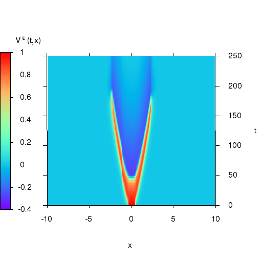
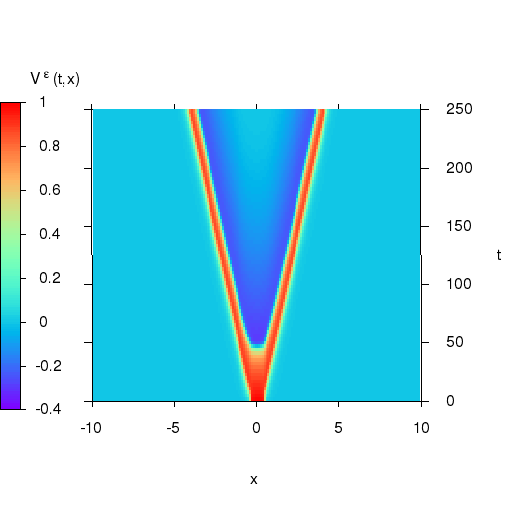
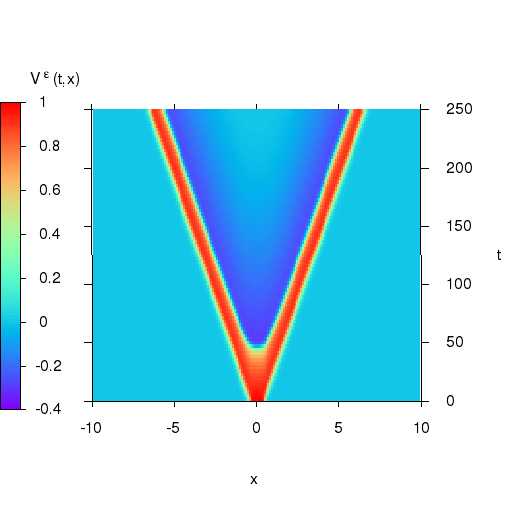
In Figure 3.1, we show the spatio-temporal profile of the mean membrane potential computed from the solution of the transport equation (1.3) for (panel (a)), (panel (b)) and (panel (c)). It shows that depending on the value of , the solution presents dramatically different dynamics. If is too large compared to the width of the considered interval, as in the case (a), two symmetric waves start to propagate, but quickly disappear, and then converges to everywhere as time goes on. On the contrary, for smaller values of as in the cases (b) and (c), that is , the function has the shape of two symmetric counter-propagating traveling pulses. This is typically the kind of slow/fast dynamics expected for the solution of (3.5) according to [7] with this set of parameters. Moreover, it seems that the speed of propagation of these waves decreases as grows, since in the case (b), the speed of propagation of these traveling pulses is slightly less than in the case (c).
Then, we display in Table 3 and 4, the numerical approximations of at fixed time for several values of for the first order (left table) and the second order (right table) numerical schemes. Since the behavior of is too different from its limit for smaller values of , we display linear regressions only from the line corresponding to . These linear regressions yield that seems to be approximately of order two in for both numerical schemes, which corresponds to the one obtained by formal computations for the continuous problem [9].
Notice that the second order numerical scheme (2.21)–(2.25) represents a negligible improvement for the speed of convergence of as goes to . A key issue in numerical analysis is to perform a similar study on the discrete solution as the one we performed on the continuous problem [9] in order to establish the asymptotic preserving property of the scheme.
3.3 Heterogeneous neuron density
In the spirit of [3, 4], the study of propagating waves in neural networks with spatial heterogeneities seems to be a fruitful topic. This subsection is therefore devoted to the illustration of the behaviour of the solution of the numerical scheme (2.17)–(2.3) with a non constant neuron density function . We choose the initial datum
with where the density is a smooth approximation of and is chosen as
| (3.7) |
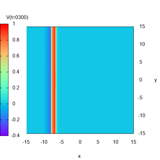
The domain in space is taken to be , discretized using points in each spatial coordinate and particles per cell. It is expected that a wave will propagate initially from the left hand side in the homogeneous density of neurons. Then in the center of the domain, the density becomes inhomogeneous, which will perturb the wave propagation front. In Figure 3.2, we propose different scenario depending on the scaling parameter . We display the profile of the solution at time , and for , and . Clearly, the amplitude of the scaling parameter has an influence on the shape of the pulse but also on the speed of propagation.
First of all, the scrolling wave does not propagate through the ball , since the neuron density is too weak. Then, we can observe that as grows small, the speed of propagation and the width of the scroll wave increase. Thus, the heterogeneity does not have exactly the same effect. For and for example, the width of the gap in the neuron density is too large compared to the width of the traveling pulse. Therefore, the scroll wave breaks at its middle, and then recomposes once the heterogeneity is passed. Then, for smaller values of , as , the traveling pulse starts to wrap the area where it cannot propagate before breaking and recomposing.
 |
 |
 |
 |
 |
 |
 |
 |
 |
| (a) | (b) | (c) |
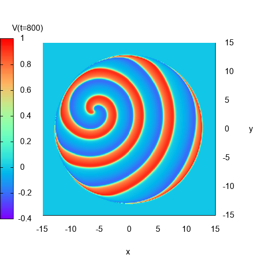
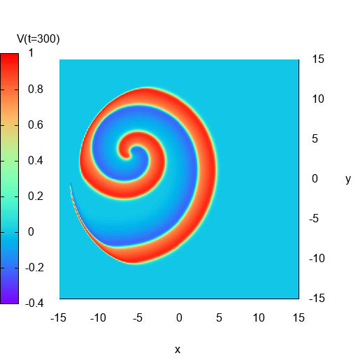
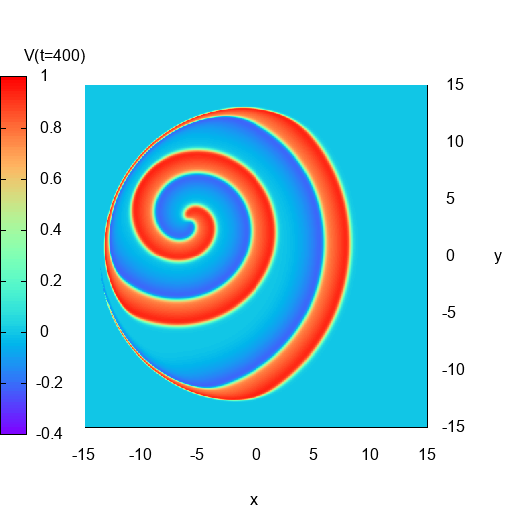
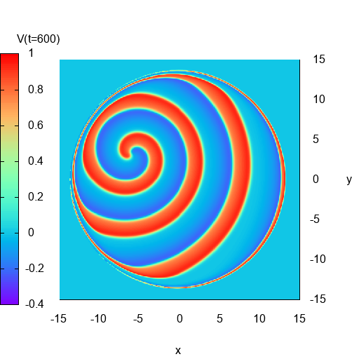
3.4 Rotating spiral waves
A spiral wave in the broadest sense is a rotating wave traveling outward from a center. Such spiral waves have been observed in many biological systems [33], [27], such as mammalian cerebral cortex [21]. Although circular waves were predicted from early models of cortical activity [2], true spiral wave formation has been already obtained in numerical simulations of reaction-diffusion systems such as the Wilson–Cowan system [32, 5].
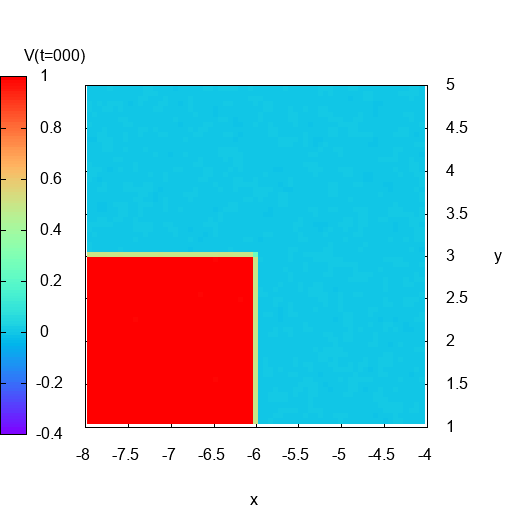
In this section, we present numerical evidence for stable spiral waves considering the transport equation (1.3)–(1.4). We choose the initial datum [5]
with where the density is a smooth approximation of the characteristic function on the disk centered in with radius , whereas is chosen as
| (3.8) |
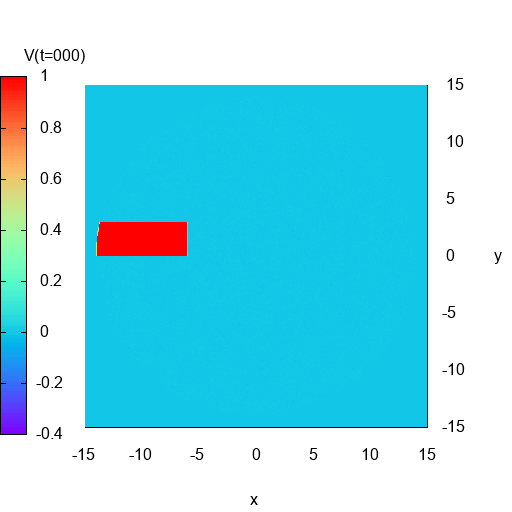
Here the trivial state is perturbed by setting the lower-left quarter of the domain to and the upper half part to , which allows the initial condition to curve and rotate clockwise generating the spiral pattern. The domain in space is taken to be , discretized using points in each spatial coordinate and particles per cell.
 |
 |
| (a) | (c) |
 |
 |
| (c) | (d) |
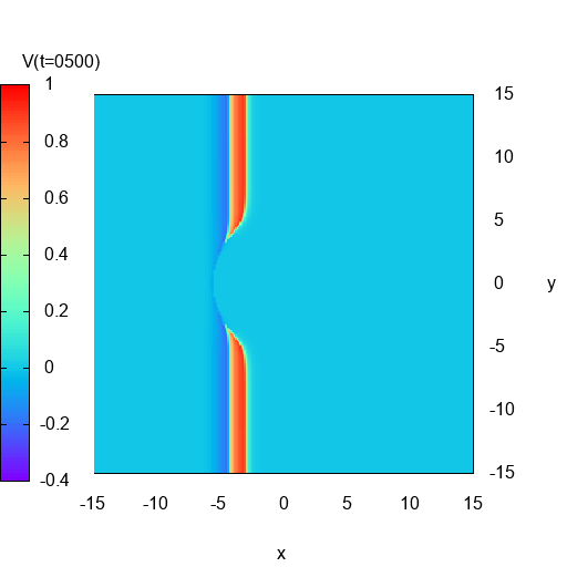
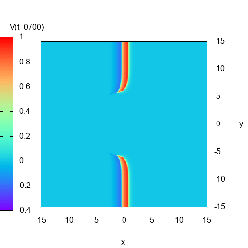
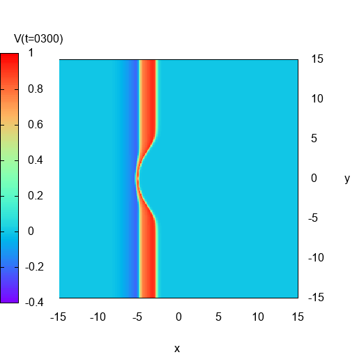
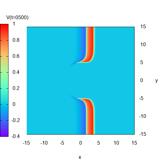
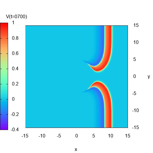
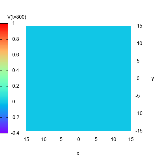
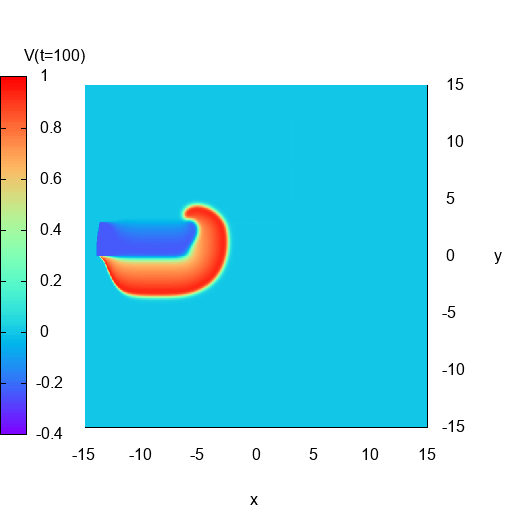
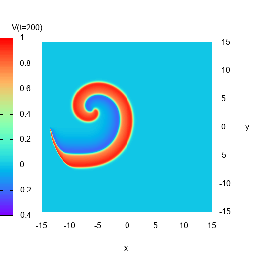
We first perform several computations changing the value of the scaling parameter and report in Figure 3.3, the profile of the numerical solution obtained using the second order scheme (2.21)–(2.23) at the final time of the simulation . On the one hand, when , we observe that the initial wave first propagates into the domain, then it is damped and the solution converges to the stable steady state when times goes on (see Figure 3.3 (a) at time ). On the other hand, when becomes smaller , the solution evolves in a different manner. Indeed, the initial wave propagates into the physical domain where , and a spiral wave appears at time , where a traveling pulse emerges and propagates from the bottom left quarter of the domain, towards the bottom right quarter, which creates a rotating spiral wave at larger time. For these values of , the shape of the solution is very sensitive to (see for instance and in Figure 3.3). Finally, when , a spiral wave appears and it seems that the solution is not anymore sensitive to .
 |
 |
 |
| (a) | (b) | (c) |
 |
 |
 |
| (d) | (e) | (f) |
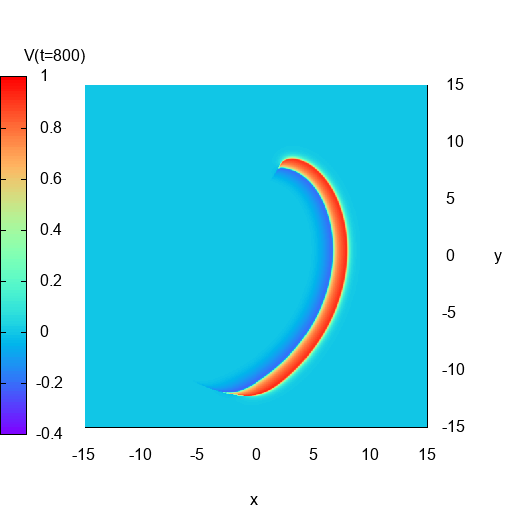
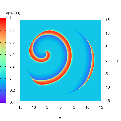
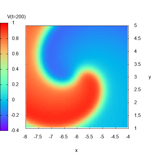
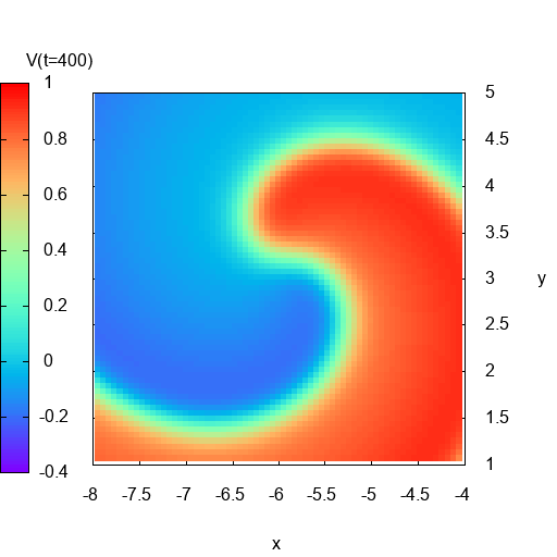
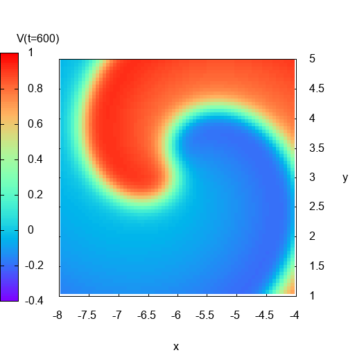
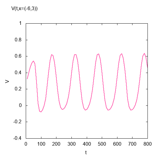
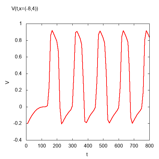
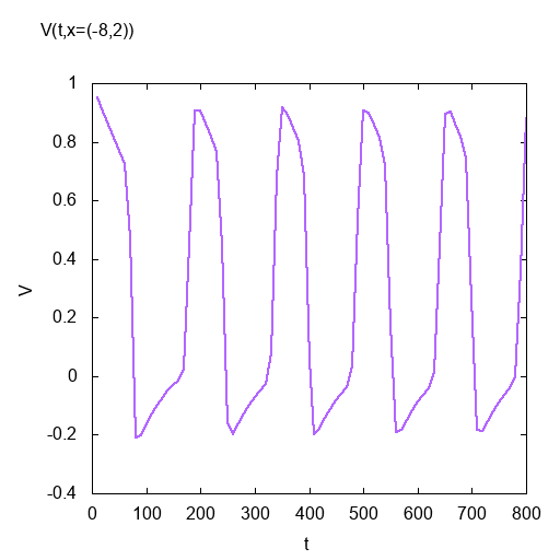
In Figure 3.4, we report the numerical results for at different time . It illustrates how the spiral wave is generated from the initial data: a traveling pulse appears and begins to rotate clockwise, while the waves propagate up to the edge of the region where . Moreover, it seems that once the spiral wave has appeared, its speed of rotation remains constant (see in (e) and (f) in Figure 3.4). Furthermore, in Figure 3.5, we report a zoom in the region where the traveling pulse appears. We observe that the center of the spiral moves and oscillates around a point. Finally in Figure 3.6, we propose the time evolution of the solution at different points , and . Close to the point , around which the spiral oscillates, time oscillations appear with an amplitude between and whereas in the neighboring points, different oscillations appear with a larger amplitude. Observe that at and , the time oscillations look the same but are shifted.
 |
 |
| (a) | (b) |
 |
 |
| (c) | (d) |
 |
 |
 |
| (a) | (b) | (c) |
4 Conclusion
In the present paper we have proposed a class of semi-implicit time discretization techniques for particle simulations to (1.3)–(1.4) coupled with a spectral collocation method for the space discretization. The main feature of our approach is to guarantee the accuracy and stability on slow scale variables even when the amplitude of local interactions becomes large, thus allowing a capture of the correct behavior with a large time step with respect to . Even on large time simulations the obtained numerical schemes also provide an acceptable accuracy on the membrane potential when , whereas fast scales are automatically filtered when the time step is large compared to .
As a theoretical validation we have proved that under some stability assumptions on numerical approximations, the slow part of the approximation converges when to the solution of a limiting scheme for the asymptotic evolution, that preserves the initial order of accuracy. Yet a full proof of uniform accuracy remains to be carried out in the frame of the continuous case [9]. The main challenge is to rigorously study the stability of the numerical solution for an appropriate norm and to find a bound uniformly with respect to and .
Acknowledgements
The authors acknowledge support from ANITI (Artificial and Natural Intelligence Toulouse Institute) Research Chair and the project ChaMaNe (ANR-19-CE40-0024).
References
- [1] S. Boscarino, F. Filbet and G. Russo, High order semi-implicit schemes for time dependent partial differential equations, J. Sci. Comput., 68 (3), (2016), pp. 975–1001.
- [2] R. L. Beurle, Properties of a mass of cells capable of regenerating pulses, Philos. Trans. R. Soc. London B, Biol. Sci. 240 (669), (1956) pp. 55–94.
- [3] P. C. Bressloff, Traveling fronts and wave propagation failure in an inhomogeneous neural network, Physica D, 155, (2001), pp. 83–100.
- [4] P. C. Bressloff, From invasion to extinction in heterogeneous neural fields , The Journal of Mathematical Neuroscience, 2, (2001).
- [5] A. Bueno-Orovio, K. Burrage and D. Kay, Fourier spectral methods for fractional-in-space reaction-diffusion equations, BIT, 54 (4), (2014), pp. 937–954.
- [6] C. Canuto, M. Y. Hussaini, A. Quarteroni and T.A. Zang, Spectral Methods in Fluid Dynamics, Berlin, Springer-Verlag (1987).
- [7] G. Carpenter, A geometric approach to singular perturbation problems with application to nerve impulse equations, J. Differential Equations, 23, (1977), pp. 335–367.
- [8] J. Crevat, Mean-field limit of a spatially-extended FitzHugh-Nagumo neural network, Kinetic & Related Models, 12 (6), (2019), pp. 1329–1358.
- [9] J. Crevat, Diffusive limit of a spatially-extended kinetic FitzHugh-Nagumo model, Mathematical Models and Methods in Applied Sciences, 30 (2020), no. 5, pp. 957–990.
- [10] P. Degond, Asymptotic-Preserving Schemes for Fluid Models of Plasma, Panoramas et synthèses, 39-40, (2013), pp. 1–90.
- [11] F. Filbet and G. Russo, High order numerical methods for the space non-homogeneous Boltzmann equation. J. Comput. Phys. 186 (2003), no. 2, pp. 457–-480.
- [12] F. Filbet, C. Mouhot and L. Pareschi, Solving the Boltzmann equation in . SIAM J. Sci. Comput. 28 (2006), no. 3, pp. 1029-–1053.
- [13] F. Filbet and S. Jin, An Asymptotic Preserving Scheme for the ES-BGK model of the Boltzmann equation, J. Sci. Computing, 46 (2), (2011), pp. 204–224.
- [14] F. Filbet, J. Hu and S. Jin, A numerical scheme for the quantum Boltzmann equation with stiff collision terms. ESAIM Math. Model. Numer. Anal. 46 (2012), no. 2, pp. 443–463.
- [15] F. Filbet, L. Pareschi and Th. Rey, On steady-state preserving spectral methods for homogeneous Boltzmann equations. C. R. Math. Acad. Sci. Paris, 353 (2015), no. 4, pp. 309–-314.
- [16] F. Filbet and L. M. Rodrigues, Asymptotically stable particle-in-cell methods for the Vlasov-Poisson system with a strong external magnetic field, SIAM J. Numer. Analysis, 54, (2016), pp. 1120–1146.
- [17] F. Filbet and L. M. Rodrigues, Asymptotically preserving particle-in-cell methods for inhomogeneous strongly magnetized plasmas, SIAM J. Numer. Analysis, 55 (2017), pp. 2416-2443.
- [18] R. FitzHugh, Impulses and physiological sates in theoretical models of nerve membrane, Biophysical journal, 1, (1961), pp. 445–466.
- [19] F.H. Harlow. The particle-in-cell computing method for fluid dynamics. Method in Computational Physics, 3, (1964), pp. 319–343.
- [20] J. S. Hesthaven, S. Gottlieb and D. Gottlieb. Spectral methods for time-dependent problems. Cambridge University Press, (2007).
- [21] X. Huang, X. Wu, J. Liang, K. Takagaki, X. Gao and J.Y. Wu, Spiral wave dynamics in neocortex. Neuron, 68 (5), (2010), pp. 978–990.
- [22] S. Jin, Efficient asymptotic-preserving (AP) schemes for some multiscale kinetic equations, SIAM J. Sci. Comput., 21 (2), (1999), pp. 441–454.
- [23] S. Jin, L. Pareschi and G. Toscani, Diffusive relaxation schemes for multiscale discrete-velocity kinetic equations, SIAM J. Numer. Anal., 35 (6), (1998), pp. 2405–2439.
- [24] A. Klar, An asymptotic-induced scheme for nonstationary transport equations in the diffusive limit, SIAM J. Numer. Anal., 35 (3), (1998), pp. 1073–1094.
- [25] V.I. Krinsky and A.S. Mikhailov, Rotating spiral waves in excitable media: the analytical results, Physica D, 9, (1983), pp. 346–371.
- [26] P. Lafitte and G. Samaey, Asymptotic-preserving Projective Integration Schemes for Kinetic Equations in the Diffusion Limit, SIAM Journal on Scientific Computing, 34 (2), (2012), pp. A579–A602.
- [27] J. D. Murray, Mathematical biology II: spatial models and biomedical applications, New York: Springer (2003).
- [28] J. Nagumo, S. Arimoto and S. Yoshizawa, An active pulse transmission line simulating nerve axon, Proceedings of the IRE, 50, (1962), pp. 2061–2070.
- [29] L. Pareschi and G. Russo, Numerical Solution of the Boltzmann Equation I: Spectrally Accurate Approximation of the Collision Operator, SIAM J. Numer. Analysis, 37 (4), (2000), pp. 1217–1245.
- [30] L. Pareschi and G. Russo, Efficient asymptotic preserving deterministic methods for the Boltzmann equation, Models and Computational Methods for Rarefied Flows, Lecture Series held at the von Karman Institute, Rhode St. Genèse, Belgium, 24 -28 January (2011).
- [31] P.A.Raviart, An analysis of particle methods, ”Numerical methods in fluid dynamics”, Springer, (1983), pp. 243–324.
- [32] H. R. Wilson and J. D. Cowan, Excitatory and inhibitory interactions in localized populations of model neurons Biophys J. 12, (1972), pp. 1-–24.
- [33] A. T. Winfree, The geometry of biological time, New York: Springer (2001).