Can preferential concentration of finite-size particles in plane Couette turbulence be reproduced with the aid of equilibrium solutions?

Abstract

This work employs for the first time invariant solutions of the Navier-Stokes equations to study the interaction between finite-size particles and near-wall coherent structures. We consider horizontal plane Couette flow and focus on Nagata’s upper-branch equilibrium solution (Nagata, 1990) at low Reynolds numbers where this solution is linearly stable. When adding a single heavy particle with a diameter equivalent to 2.5 wall units (one twelfth of the gap width), we observe that the solution remains stable and is essentially unchanged away from the particle. This result demonstrates that it is technically feasible to utilize exact coherent structures in conjunction with particle-resolved DNS. While translating in the streamwise direction, the particle migrates laterally under the action of the quasi-streamwise vortices until it reaches the region occupied by the low-speed streak, where it attains a periodic state of motion – independent of its initial position. As a result of the ensuing preferential particle location, the time-average streamwise particle velocity differs from the plane-average fluid-phase velocity at the same wall-distance as the particle center, as previously observed in experiments and in numerical data for fully turbulent wall-bounded flows. Additional constrained simulations where the particle is maintained at a fixed spanwise position while freely translating in the other two directions reveal the existence of two equilibria located in the low-speed and in the high-speed streak, respectively, the former being an unstable point. A parametric study with different particle to fluid density ratios is conducted which shows how inertia affects the spanwise fluctuations of the periodic particle motion. Finally, we discuss a number of potential future investigations of solid particle dynamics which can be conducted with the aid of invariant solutions (exact coherent structures) of the Navier-Stokes equations.

1 Introduction

In many natural and technical systems the interaction between fluid flow and solid particles plays an important role. Examples are the most diverse: in nature it ranges from blood flow to volcanic eruptions, whereas in industrial applications a classical example is the combustion of pulverized coal. In such systems, one aspect that is of primordial importance is the spatial distribution of the dispersed phase. It can significantly affect various quantities of practical interest, such as particle dispersion, inter-particle collision statistics, mean relative velocities and turbulence enhancement/attenuation. Nevertheless, to the present day, our understanding of the fundamental process behind structure formation in the particulate phase or about turbulence modulation due to particles is still incomplete.

A typical approach to understand fluid-particle interaction consists of analyzing data from direct numerical simulations (DNS). These analyses are often performed a posteriori and consist in operations like spatial filtering or conditional averaging in an attempt to extract the key mechanisms that govern fluid-particle interaction. Approaches of this kind have led to new observations and have advanced the knowledge on this topic quite considerably in the past decades. For example, in wall-bounded flows, heavy particles moving near a solid wall tend to concentrate in the low-speed regions and form streamwise aligned streaks. This particle preferential concentration has been observed in numerous experimental and numerical investigations, (e.g., Refs. (Yung et al., 1989; Rashidi et al., 1990; Hetsroni & Rozenblit, 1994; Kaftori et al., 1995; Niño & Garcia, 1996; Pan & Banerjee, 1997; Uhlmann, 2008; García-Villalba et al., 2012)), and it is known to depend on particle size and density. Kidanemariam et al. (2013) performed particle-resolved DNS of horizontal turbulent channel flow with a very dilute set of particles having a diameter equivalent to 7 wall units and a submerged weight which essentially restricted them to a position in contact with the lower bounding wall. Through conditional averaging they found that there is a significant statistical correlation between spanwise particle velocity and the presence of a nearby quasi-streamwise vortex with the corresponding sign of rotation. This statistical argument explains the migration to low-speed streaks which are typically flanked by counter-rotating streamwise vortices; as a consequence, the average streamwise particle velocity is lower than the mean fluid velocity at the same wall-distance due to the preferential particle concentration in low-speed regions. Despite the success of such statistical approaches it is not always straightforward to extract the salient features of a fully turbulent flow field from massive DNS data-sets, and to link the relevant flow structures to the observed particle dynamics.

An alternative to the above methods is to consider surrogate flow-fields instead of fully-developed turbulence. This has the obvious advantage of making the analysis of particle motion conceptually easier, although at the risk of being less relevant to the fully turbulent state of interest. Along this line, Maxey (2002) used a cellular flow to investigate the clustering properties of small spherical particles, and Reeks et al. (2006) considered randomized Taylor-Green vortex flow to elucidate the random uncorrelated particle motion. Of equal interest is the work of Bergougnoux et al. (2014), who set up experimentally a cellular flow to investigate the influence of vortical structures upon the settling of small particles.

Another way to simplify the problem, which has to the best of our knowledge not yet been explored, is to investigate particle motion in flow fields that are invariant solutions to the Navier-Stokes equations. These solutions are widely believed to be of relevance to full turbulence, as some of them are able to reproduce statistical features of turbulent flows; cf. Kawahara et al. (2012) for a review about the significance of invariant solutions to turbulence, and van Veen (2019) for a review on the history of invariant solutions in turbulence. Invariant solutions range from simple fixed points (equilibrium states), which are time invariant in some suitable frame of reference, to more complex and dynamic flow fields that recur at a fixed time period (periodic orbits). Solutions of this type have been found in various flow configurations, such as plane Couette flow (Nagata, 1990), plane Poiseuille flow (Waleffe, 2001), Hagen-Poiseuille flow (Faisst & Eckhardt, 2003), or square-duct flow (Uhlmann et al., 2010; Okino et al., 2010). In the present contribution we focus on plane Couette flow, which on one hand is a wall-bounded flow with far-reaching applications, and for which, on the other hand, well-known solutions exist.

Equilibrium states for plane Couette flow have traditionally been found through homotopy techniques, i.e. by embedding the problem of interest into a generalized configuration: Nagata (1990) used spanwise rotation, Clever & Busse (1992) resorted to wall heating, and Waleffe (1998) imposed an artificial body force. Nagata’s solution originates from a saddle-node bifurcation at a finite Reynolds number, and it can be continued along a lower and an upper solution branch, both of which extend to high-Reynolds numbers. The upper branch of the solution is believed to be of relevance for the turbulent state: the coherent structures embedded therein, i.e. a pair of counter-rotating streamwise vortices flanking a wavy low-speed streak, emulate well the coherent structures typically found in the turbulent buffer layer, and the velocity profiles of these solutions also resemble those typically found in turbulent wall-bounded flows (Jiménez et al., 2005). Let us mention in passing that periodic orbits containing a full regeneration cycle of vortices and velocity streaks have been detected in plane Couette flow by Kawahara & Kida (2001) and others.

Thus, some of the known invariant solutions, more specifically equilibrium solutions, provide exact coherent structures that are of relevance to turbulence, like an apparatus in a laboratory that would contain some of the main ingredients of turbulence (Kerswell, 2005), albeit typically at low Reynolds number. This unique trait is appealing for the study of the effects of coherent vortices on particle dynamics, as it makes the problem more amenable by untangling turbulence and isolating its building blocks. However, this approach is technically not trivial as the presence of a solid phase can disturb the equilibrium state and lead to re-laminarization or transition to turbulence. In a first step towards introducing the concepts of invariant solutions into the study of finite-size particle motion, the present work considers the question whether simple invariant solutions seeded with finite-size particles can be used to study the interaction between finite-size particles and true turbulence. To this end, we address the following specific questions in the context of plane Couette flow:

1. How long can equilibrium solutions be observed once finite-size particles have been added?

2. Do equilibrium solutions seeded with finite-size particles exhibit preferential particle concentration?

In Section 2 we describe the flow configuration, present the numerical methodology, and define the physical and numerical parameters of this study. In the sequence (Section 3), we compute a set of equilibrium solutions and study their stability. Finally, in Section 4, we add finite-size particles to these plane Couette flow equilibria and study the ensuing temporal evolution of the system.

2 Numerical Set-up

2.1 Flow configuration and parameters

We consider plane Couette flow with two parallel walls, which are separated by a distance $2h$, and extend in the $x$ and $z$ directions by $\mathcal{L}_{x}$ and $\mathcal{L}_{z}$, such that the physical domain is defined as $\boldsymbol{\Omega}=[0,\mathcal{L}_{x}]\times[-h,h]\times[0,\mathcal{L}_{z}]$ (cf. Fig. 1). The walls move in the $x$-direction with speed $U$, and their counter movement induces shear and drives the flow. A gravitational field $\mathbf{g}$ acts in the negative wall normal direction with intensity $g$.

The fluid motion is governed by the incompressible Navier-Stokes equations, viz.

$$\nabla\cdot\mathbf{u}_{f}=0,$$ (1)

$$\frac{\partial\mathbf{u}_{f}}{\partial t}+(\mathbf{u}_{f}\cdot\nabla)\,\mathbf{u}_{f}=-\frac{1}{\rho_{f}}\nabla p+\nu\nabla^{2}\mathbf{u}_{f},$$ (2)

where, $\mathbf{u}_{f}=(u_{f},v_{f},w_{f})$ is the fluid velocity, $p$ is the hydrodynamic pressure, $\nu$ is the kinematic viscosity of the fluid and $t$ denotes time. The flow field $\mathbf{u}_{f}$ satisfies a no-slip boundary condition at the two solid walls and at the fluid/particle interface. The flow field is assumed periodic in the $x$ and $z$ directions with streamwise and spanwise wavelengths $\lambda_{x}=\mathcal{L}_{x}$ and $\lambda_{z}=\mathcal{L}_{z}$, respectively.

The motion of the solid-phase, which is formed of finite-size spherical particles of diameter $D_{p}$ and density $\rho_{p}$, is governed by the Newton-Euler equations for the motion of rigid bodies:

$$\rho_{p}V_{p}\dfrac{\mbox{d}{\mathbf{u}_{p}}}{\mbox{d}{t}}=\rho_{f}\oint_{\partial S}\boldsymbol{\tau}\cdot\mathbf{n}\,\mathrm{d}\sigma+(\rho_{p}-\rho_{f})V_{p}\mathbf{g},$$ (3)

$$I_{p}\dfrac{\mbox{d}{\boldsymbol{\omega}_{p}}}{\mbox{d}{t}}=\rho_{f}\oint_{\partial S}\mathbf{r}\times(\boldsymbol{\tau}\cdot\mathbf{n})\mathrm{d}\sigma.$$ (4)

Here $\mathbf{u}_{p}=(u_{p},v_{p},w_{p})$ is the linear particle velocity, $\boldsymbol{\omega}_{p}$ is the angular particle velocity, $\boldsymbol{\tau}=-p\,\mathbf{I}+2\nu(\mathbf{u}_{f}+\mathbf{u}_{f}^{T})$ is the hydrodynamic stress with $\mathbf{I}$ the identity tensor and $\mathbf{r}$ the position vector with respect to the particle’s centroid. The vector normal to the fluid-solid interface $\partial S$ is denoted by $\mathbf{n}$, and the volume and the moment of inertia of the particles are $V_{p}$ and $I_{p}$, respectively. At the fluid/particle interface $\partial S$, a no-slip boundary condition is imposed through an immersed boundary method as further explained in Section 2.2.3 and in Appendix A. Particle-wall contact is assumed to be frictionless, as in the DNS of Kidanemariam et al. (2013). Particles can, therefore, slide without additional tangential stress along the horizontal walls.

In its most general form, our numerical experiments involve a total of $9$ control parameters that need to be prescribed: $\{\rho_{p},\rho_{f},\nu,\mathcal{L}_{x},\mathcal{L}_{z},h,D_{p},U,g\}$. This specific set may be combined into a group of $6$ independent non-dimensional numbers. These are taken as the dimensionless geometrical dimensions $\mathcal{L}_{x}/h$ and $\mathcal{L}_{z}/h$, the Reynolds number based on the absolute wall speed and on half of the wall separation $Re=Uh/\nu$, the density ratio $\rho_{p}/\rho_{f}$, the non-dimensional particle diameter $D_{p}/h$ and the Galileo number $Ga=u_{g}D_{p}/\nu$, where $u_{g}=\sqrt{(\rho_{p}/\rho_{f}-1)gD_{p}}$ is the gravitational velocity.

The box-averaged energy dissipation rate $\mathcal{E}_{D}$, is defined as

$$\mathcal{E}_{D}=\frac{h^{2}}{U^{2}}\langle\boldsymbol{\omega}_{f}\cdot\boldsymbol{\omega}_{f}\rangle_{xyz},$$ (5)

where $\boldsymbol{\omega}_{f}$ denotes the fluid vorticity, and $\langle\,\cdot\,\rangle_{xyz}$ is the spatial average over the three spatial directions. Note that the dissipation defined in (Eq. 5) is normalized such that the laminar flow solution yields $\mathcal{E}_{D}=1$. The instantaneous wall shear stress, averaged over each of the two wall planes, is defined as:

$$\tau_{w,l}=\rho_{f}\nu\,\frac{\partial\langle u_{f}\rangle_{xz}}{\partial y}\Bigr{|}_{y=-h}\quad\text{and}\quad\tau_{w,u}=\rho_{f}\nu\,\frac{\partial\langle u_{f}\rangle_{xz}}{\partial y}\Bigr{|}_{y=+h}$$ (6)

where $\langle\,\cdot\,\rangle_{xz}$ denotes the two-dimensional spatial averaging operator. By defining the mean friction velocity as $u_{\tau}=\sqrt{(\tau_{w,l}+\tau_{w,u})/(2\rho_{f})}$, the viscous lengthscale is given by $\delta_{\nu}=\nu/u_{\tau}$, and the friction-velocity-based Reynolds number is $Re_{\tau}=u_{\tau}h/\nu$. Henceforth the standard notation with a “$+$” superscript refers to quantities normalized with these viscous wall units. The bulk velocity is defined as

$$u_{b}=\frac{1}{h}\int_{0}^{h}\langle u_{f}\rangle_{xz}(y)\mathop{}\!\mathrm{d}{y}\,,$$ (7)

which lets us define a bulk flow time scale $\tau_{b}=h/u_{b}$.

The responsiveness of particles to fluid forcing is typically measured through the Stokes number, i.e. the ratio between particle and fluid time scales. Taking the particle response time based on the Stokes drag $\tau_{p}=D_{p}^{2}\rho_{p}/(18\nu\rho_{f})$, we define a first Stokes number based on bulk time units $St_{b}=\tau_{p}/\tau_{b}$ and a second Stokes number $St^{+}=\tau_{p}/\tau_{\nu}$ based on the viscous time-scale $\tau_{\nu}=\delta_{\nu}/u_{\tau}$.

Spatial fluctuations of flow quantities around the wall-parallel plane average are defined as follows, e.g. for the fluid velocity: $\mathbf{u}_{f}^{\prime}=\mathbf{u}_{f}-\langle\mathbf{u}_{f}\rangle_{xz}$. From these we define second moments such as the box-averaged kinetic energy of the fluctuations $K=\langle\mathbf{u}_{f}^{\prime}\cdot\mathbf{u}_{f}^{\prime}\rangle_{xyz}/2$, and the plane-averaged velocity variances, e.g. in the streamwise direction $\langle u_{f}^{\prime}u_{f}^{\prime}\rangle_{xz}$. We will also employ time-averaging which is indicated through the use of the operator $\langle\,\cdot\,\rangle_{t}$ with the averaging interval being made more precise below.

2.2 Numerical methods

The numerical approach employed in this study involves three different methodologies based on separate code frameworks. First, we use a Newton-Raphson solver to find equilibrium solutions of the Navier-Stokes equations in plane Couette flow. Second, the stability of the equilibrium states are tested with the aid of a pseudo-spectral DNS solver. Third, a DNS finite-difference code coupled with the Newton/Euler equations of rigid particle motion is employed for time marching equilibrium solutions seeded with finite-size particles. In the following we briefly describe the different numerical methods.

2.2.1 Equilibrium solutions

Equilibrium solutions are solenoidal velocity fields $\mathbf{u}_{f}^{eq}$ that satisfy the condition ${\partial{\mathbf{u}_{f}^{eq}}}/{\partial{t}}=0$ in Eq. 2 for a given $Re$, $\lambda_{x}$ and $\lambda_{z}$. The present methodology is essentially equivalent to the one of Ehrenstein & Koch (1991) which uses the Laplacian of the wall-normal velocity perturbation and the wall-normal vorticity perturbation as unknowns, and which employs Fourier series expansions and Chebyshev polynomials for the spatial discretization. The resulting non-linear set of equations is solved iteratively through a Newton-Raphson method. In order to track solutions in the $Re$, $\lambda_{x}$ and $\lambda_{z}$ parameter space, an arc-length continuation method is employed (Keller, 1977). The numerical code used in this part of the study is the same as used in Jiménez et al. (2005), and we refer the reader to the latter reference for more details.

2.2.2 Stability analysis

In order to investigate the stability of equilibrium solutions (in the absence of solid particles) we perform a time-stepping-based stability analysis where white noise is added to $\mathbf{u}_{f}^{eq}$, and the disturbed velocity field is advanced in time by a pseudo-spectral DNS code. If the disturbances are amplified in time, the parameter point is regarded as unstable. On the other hand, if the disturbances are damped in time, the parameter point is considered stable. The white noise that is added to each degree of freedom is of the form $A\exp(I\theta)$, where $I$ is the unit imaginary number, $\theta\in[0,2\pi]$ is a random phase and $A$ is the amplitude of the disturbance. The employed numerical algorithm is as described by Kim et al. (1987). It solves the governing equations using again a pressure-free formulation, where the dependent variables are the Laplacian of the wall-normal velocity and the wall-normal vorticity. The unknowns are expanded with Fourier/Chebyshev series, and a three-step low-storage Runge-Kutta scheme is used for time integration. The code is essentially the same as the one used in Jiménez & Pinelli (1999) with slight modifications for the Couette flow boundary conditions.

2.2.3 Interface-resolved particulate flow solver

In order to solve the set of equations (Eq. 1-Eq. 4) for the coupled motion of fluid and particles we resort to an immersed boundary technique. A body force term $\mathbf{f}^{ibm}$ is introduced on the right-hand-side of the momentum equation (Eq. 2) which is formulated such that the no-slip condition is enforced at the particle surface. The specific formulation is the one proposed by Uhlmann (2005) which is reproduced in appendix Appendix A for convenience. A standard fractional step method is employed, and the spatial gradients are discretized through central, second-order finite-differences on a staggered mesh. The temporal discretization is performed with a Crank-Nicolson scheme for the viscous terms and a three-step Runge-Kutta scheme for advection. The particle motion (Eq. 3-Eq. 4) is explicitly coupled to the solution of the Navier-Stokes equations (Eq. 1-Eq. 2). The Poisson equation for the pseudo-pressure is solved with the aid of a multigrid technique; the Helmholtz problems for the velocity prediction are solved with an approximate factorization technique. The numerical code uses three-dimensional Cartesian domain decomposition for parallelism on distributed memory systems. The particle-wall interaction is treated with a simple repulsive force method (Glowinski et al., 1999), as in the DNS study of Kidanemariam et al. (2013); no tangential (frictional) contact force is imposed. For the two-phase flow simulations the computational grid is uniform and isotropic due to requirements for consistency of the immersed boundary method. This condition is however relaxed for the single-phase simulations. The numerical algorithm is described in detail in Uhlmann (2005) and has been used in a number of previous studies, e.g. (Uhlmann, 2008; Kidanemariam et al., 2013; Uhlmann & Doychev, 2014; Chouippe & Uhlmann, 2015).

3 Tracking Equilibrium Solutions

Before considering particulate flows, we need to establish the relevant single-phase equilibrium solutions as well as their stability properties.

3.1 Nagata’s solutions

We restrict our search to Nagata-like solutions as these have been extensively studied in the literature. We consider solutions with different values of the Reynolds number $Re$, and with different fundamental wavenumbers $\lambda_{x}$ and $\lambda_{z}$. For this purpose we use two different computational domains $\boldsymbol{\Omega}_{1}$ and $\boldsymbol{\Omega}_{2}$, the latter one being twice as large in both the streamwise and the spanwise direction (cf. Tab. 1).

First we have continued one of Nagata’s solutions previously used in Jiménez et al. (2005) with respect to the fundamental wavelengths $\lambda_{x}$ and $\lambda_{z}$ until it matched the size of the target domains $\boldsymbol{\Omega}_{1}$ and $\boldsymbol{\Omega}_{2}$. Then continuation in terms of $Re$ was performed with $16\times 32\times 16$ Fourier-Chebyshev-Fourier coefficients, and equilibrium states of interest were recomputed with $48\times 49\times 48$ coefficients ($112\,896$ degrees of freedom). We have verified that this numerical resolution is sufficient to resolve the highest coefficients of the Fourier-Chebyshev-Fourier representation up to machine precision for all $Re$ numbers that are considered here.

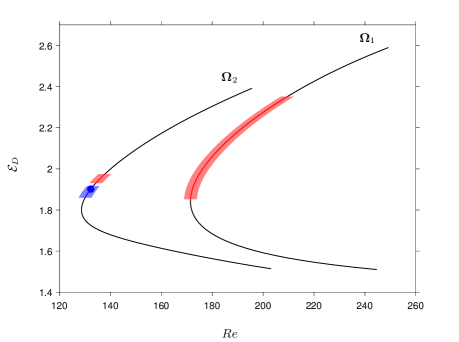
Figure 2: State-space diagram for Nagata’s solution in terms of the energy dissipation rate $\mathcal{E}_{D}$ and the Reynolds number. (a) Domain $\boldsymbol{\Omega}_{1}$ with $(\lambda_{x},\lambda_{z})=(6h,3h)$; (b) domain $\boldsymbol{\Omega}_{2}$ with $(\lambda_{x},\lambda_{z})=(12h,6h)$, where $\lambda_{x}$ and $\lambda_{z}$ are the fundamental wavelengths in the streamwise and spanwise directions. The blue (red) shading indicates stability (instability) of the solution, as determined in LABEL:{sec:stab-analysis}. The blue dot on the upper branch of the solution in box $\boldsymbol{\Omega}_{2}$ marks the selected parameter point for the present study.

The average dissipation rate of the single-phase flow solutions is shown in Fig. 2 for both sets of fundamental wavenumbers. It can be observed that for these parameters, the branches originate at the critical Reynolds number $171.45$ ($128.61$) in domain $\boldsymbol{\Omega}_{1}$ ($\boldsymbol{\Omega}_{2}$). The upper branches feature substantially larger values of the dissipation rate which indicates the presence of finer scales, i.e. steeper spatial velocity gradients. Note that many previous authors have computed Nagata-type solutions for plane Couette flow (e.g. Waleffe, 2003; Gibson et al., 2009); however, we re-computed them here for convenience and for having precise control over the cell size. In the following we focus upon equilibrium solutions on the upper-branch, as they are directly related to the turbulent state (Jiménez et al., 2005), as further discussed in Section 3.3.

3.2 Stability analysis

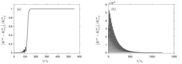
Figure 3: Example of the stability analysis showing an unstable and a stable equilibrium solution. In (a) we see that for domain $\boldsymbol{\Omega}_{1}$ and $Re=190.62$ the initial disturbances get amplified with time and that after approximately $200\,\tau_{b}$ the laminar base flow is recovered. In (b) the initial disturbance in domain $\boldsymbol{\Omega}_{2}$ with $Re=132.25$ is continuously damped and the unperturbed case is recovered for $t>1000\,\tau_{b}$.

In order to determine the stability of the equilibrium solutions, we added white noise with an amplitude $A=10^{-5}\,U$ (cf. Section 2.2.2). Each of these perturbed solutions were integrated in time using the pseudo-spectral time-stepper, and, in total, we analyzed $10$ ($6$) parameter points on the upper-branch of domain $\boldsymbol{\Omega}_{1}$ ($\boldsymbol{\Omega}_{2}$). The stability of each parameter point was judged based on the box-averaged kinetic energy of the fluctuations. Note that the superscript “$ps$” indicates a quantity computed with the aid of the pseudo-spectral time-stepper, whereas the unperturbed kinetic energy is denoted as $K^{ps}_{ref}$. The cases in which the perturbation caused the system to move away from its equilibrium value were regarded as unstable, and otherwise as stable. As an example, Fig. 3(a) shows an unstable parameter point leading to the laminar state, and Fig. 3(b) shows a stable one. Our analysis reveals that all the investigated parameter points of domain $\boldsymbol{\Omega}_{1}$ are unstable, whereas the upper-branch of domain $\boldsymbol{\Omega}_{2}$ is stable within a narrow $Re$ region in the proximity of the turning point. The results of this stability analysis are summarized by the shaded areas in Fig. 2, and the specific results are documented in Appendix B. Although, we did not perform a sensitivity study by varying the amplitude of the initial perturbation, we have also applied the same procedure to successfully reproduce the results of Clever & Busse (1997). In that study, the authors show that the upper-branch of Nagata’s solutions with $(\lambda_{x},\lambda_{z})=(4\pi h,2\pi h)$ is indeed stable for $Re$ in the vicinity of $Re_{min}$.

Note that the above analysis does not take into account possible instability with respect to sub-harmonic perturbations, since we perform the DNS in a domain which is commensurate with the fundamental harmonic of Nagata’s solution (i.e. with $L_{x}=\lambda_{x}$ and $L_{z}=\lambda_{z}$).

3.3 Characteristics of the selected equilibrium solution

For the remainder of this work we select as our principle parameter point the solution at $Re=132.25$ on the upper branch of domain $\boldsymbol{\Omega}_{2}$ (cf. Tab. 2 for precise values of the physical parameters).

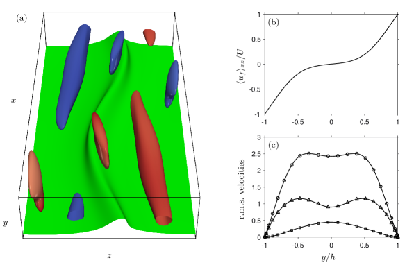
Figure 4: Upper branch of Nagata’s solutions at $Re=132.25$ and $(\lambda_{x},\lambda_{z})=(12h,6h)$. (a) Iso-surfaces: $u=\text{min}\,u(x,y=0,z)$ (green); Q-criterion of Hunt et al. (1988) with $Q=0.7\,\text{max}(Q)$, colored according to the sign of the streamwise vorticity, i.e. $\omega_{x}<0$ (blue) and $\omega_{x}>0$ (red). (b) Mean streamwise velocity normalized by the wall speed. (c) Root mean square velocities in wall units: $\langle u_{f}^{\prime}u_{f}^{\prime}\rangle_{xz}^{1/2}/u_{\tau}$ (  ); $\langle v_{f}^{\prime}v_{f}^{\prime}\rangle_{xz}^{1/2}/u_{\tau}$ (  ); $\langle w_{f}^{\prime}w_{f}^{\prime}\rangle_{xz}^{1/2}/u_{\tau}$ (  ).

In order to provide insight into the structure of the chosen single-phase flow field, we show in Fig. 4(a) iso-surfaces of the Q-criterion of Hunt et al. (1988) colored according to the sign of streamwise vorticity, plotted alongside iso-surfaces of the streamwise velocity. It can be seen that a wavy low-speed streak is flanked by counter-rotating vortices resembling the coherent structures typically found in near-wall turbulence. These features are present despite the low value of the friction Reynolds number $Re_{\tau}=15.87$.

The corresponding wall-normal profiles of the mean streamwise velocity and of the standard deviations of velocity (all with respect to the wall-parallel plane average) for this solution are shown in Fig. 4(b,c). It can be seen that these low-order moments of the velocity field exhibit the qualitative features of their statistical counterparts found in turbulent flows (Bech et al., 1995), e.g. a representative anisotropy and a distinct peak of the streamwise fluctuation intensity.

4 Exact Coherent Structures and Finite-Size Particles

Let us now turn to the main part of this work by adding finite-size particles to the previously selected single-phase solutions. Particles are inserted into the fluid domain with their initial velocity set equal to that of the unperturbed fluid at the initial position of the particle’s centroid. In total, we have conducted 15 independent simulations with physical parameters as listed in Tab. 3. While the particle diameter is set to $D_{p}/h=0.156$ ($D_{p}^{+}=2.48$) throughout this work, we consider a range of density ratios $\rho_{p}/\rho_{f}$ in order to explore the effect of particle inertia.

The chosen number of grid nodes is $768\times 128\times 384$ except where stated otherwise. The uniform isotropic grid spacing is therefore equivalent to $\Delta x^{+}=\Delta y^{+}=\Delta z^{+}=0.25$ which in turn corresponds to a particle resolution of $D_{p}/\Delta x=10$. Note that we have checked that the results do not change significantly when refining the grid by a factor of $2/3$, i.e. with a grid comprising $1152\times 193\times 576$ nodes and a particle resolution of $D_{p}/\Delta x=15$. Details on this refinement study are presented in Appendix D.

4.1 Single particle

Let us first consider case S10 which features a single particle with density ratio $\rho_{p}/\rho_{f}=10$, corresponding to a wall-unit-based Stokes number of $St^{+}=3.41$.

The particle is released at an arbitrary position in the vicinity of the bottom wall, after which the simulation is run for a total duration of $T_{obs}=1500\,\tau_{b}$. Based on the resulting data we can now address the main questions laid out in the introduction of this study: does the presence of a single-particle disturb the equilibrium solution significantly? Does the particle motion exhibit preferential concentration with respect to the coherent flow structures?

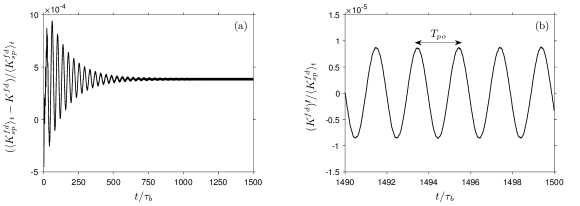
Figure 5: (a) Time evolution of the difference between the box-averaged kinetic energy in the single-phase case ($\langle K^{fd}_{sp}\rangle_{t}$) and in run S10 ($K^{fd}$). (b) Zoom of the fluctuations of the box-averaged kinetic energy, $(K^{fd})^{\prime}$, around its mean value in the periodic regime, shown for the final few cycles of case S10.

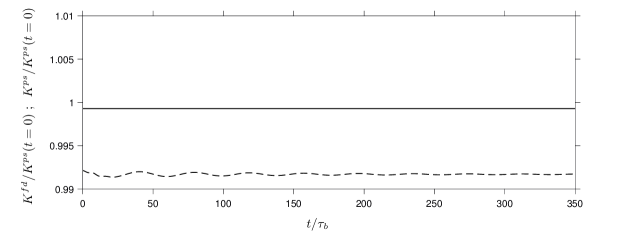
Figure 13: Time evolution of the box-averaged kinetic energy of the fluctuations for Nagata’s solution with $(\lambda_{x},\lambda_{z})=(12h,6h)$ and $Re=132.25$ when integrated using a pseudo-spectral time-stepper as described in Section 2.2.2 (  ) and with the second-order finite-difference solver as described in Section 2.2.3 with a uniform grid featuring widths of $(\Delta x^{+},\Delta y^{+},\Delta z^{+})=(0.50,0.25,0.50)$, starting from a spectrally interpolated solution at time $t=0$ (  ).

Remarkably, it turns out that the presence of the finite-size solid particle does not disfigure the equilibrium state, and Nagata’s solution is surprisingly well preserved even after $1500\,\tau_{b}$. First, in Fig. 5a we compare the time evolution of kinetic energy in case S10 with the corresponding results from the single-phase simulation (Fig. 13). Here the reference single-phase solution is represented by its time averaged value in the interval $300<t/\tau_{b}<350$, $\langle K^{fd}_{sp}\rangle_{t}$ (where the subscript “$sp$” was added to denote single-phase). It is observed that the signal exhibits a damped oscillation which decays on the order of ${\cal O}(10^{3})$ bulk time units, finally yielding a sinusoidal periodic signal (cf. Fig. 5b). The period of the signal in the asymptotic state is $T_{po}=2.04\,\tau_{b}$, and the amplitude of its fluctuations only measures approximately $10^{-5}$ times the mean kinetic energy of the unperturbed flow field, $\langle K^{fd}_{sp}\rangle_{t}$. The discrepancy in the mean value of kinetic energy induced by the presence of the single particle is marginal and on the order of $10^{-4}\langle K^{fd}_{sp}\rangle_{t}$, thus indicating that Nagata’s solution is essentially preserved at this parameter point. This observation is also confirmed by flow visualization, which yields largely consistent structures as in the single-phase case (cf. Fig. 4), and which has therefore been omitted here. A refined analysis shows that the introduction of the particle triggers a very slight unsteadiness of the macroscopic flow field, which corresponds to Nagata’s solution moving in the negative $x$-direction with a tiny propagation velocity equal to $-2.33\cdot 10^{-4}u_{b}$. This result has been verified under the above mentioned grid refinement.

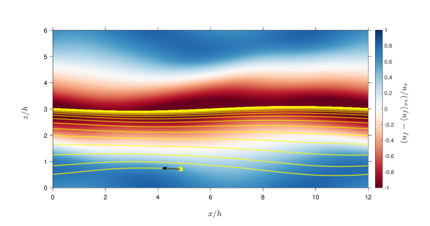
Figure 6: Iso-contours of fluctuations of the streamwise fluid velocity in an $(x,z)$-plane that intersects the particle centroid. The iso-contours evidence the presence of a low-speed streak centered around $z/h=3$. Note that the depicted flow field corresponds to the unperturbed flow. The yellow circle denotes the initial particle position. The dotted line indicates the trajectory of the particle over the course of the simulation.

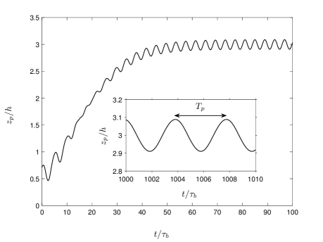
Figure 7: Spanwise particle position over time in bulk units for run S10. The inset shows a zoom of the data in the asymptotic regime, when the motion is periodic with period $T_{p}=3.93\,\tau_{b}$ and an amplitude of $0.09\,h$.

Let us now turn to the particle dynamics. We observe that the particle moves in the (negative) streamwise direction at roughly the speed of the surrounding fluid. Due to the action of the spanwise velocity induced by the quasi-streamwise vortices, it slowly drifts towards the spanwise center of the domain, approaching the low-speed fluid region (cf. Fig. 6). Meanwhile, the wall-normal motion of the particle is insignificant, and it remains near its initial wall-normal position during the course of the simulation, as expected from its large Galileo number value. By following the particle’s spanwise position (Fig. 7), we observe that it takes about $50\,\tau_{b}$ for the particle to reach the region occupied by the low-speed streak (around $z_{p}/h=3$). Subsequently, the spanwise particle position attains a state with a purely sinusoidal oscillation with amplitude $0.09\,h$ and period $T_{p}=3.93\,\tau_{b}$, as can be seen from the inset in Fig. 7. The average streamwise particle velocity measures $\langle u_{p}\rangle_{ft}=-0.94\,U$, and the time for one particle flow-through ($\mathcal{L}_{x}/\langle u_{p}\rangle_{ft}$) matches with the period of the spanwise oscillatory motion $T_{p}$.

As a consequence of the preferential location of the particle in the low-speed streak, it turns out that the time-average particle velocity in the asymptotic state significantly differs from the corresponding average fluid velocity. Let us define an apparent velocity lag as follows

$$u_{lag}=\langle u_{f}\rangle_{xz}(y=-h+D/2)-\langle u_{p}\rangle_{ft}\,.$$ (8)

Here we obtain a value of $u_{lag}=1.1\,u_{\tau}$ which is comparable to what has been observed in DNS of turbulent horizontal channel flow by Kidanemariam et al. (2013): these authors’ particles with diameter $D^{+}=7$ in a flow with $Re_{\tau}=185$ exhibited an apparent velocity lag of approximately $2\,u_{\tau}$ when located in the immediate vicinity of the wall. Let us underline that the apparent lag does not reflect the relative velocity seen by the particle, but that it is a consequence of the separate averaging of each phase in equation (Eq. 8), and, therefore, that it reflects the statistical bias due to preferential particle concentration.

It is also noteworthy that the mechanism of particle migration is caused by the spanwise flow velocity induced by the quasi-streamwise vortices. Consequently the spanwise particle motion is essentially due to the hydrodynamic drag force which can be modeled by standard quasi-steady drag formulae (Clift et al., 1978). It should then in principle be possible to obtain a fair reproduction of the present results in the context of a point-particle approach, i.e. without resolving the flow around the suspended rigid particle (Balachandar & Eaton, 2010), and to use the present set-up as a testbed for such models. It appears worthwile to further explore this avenue in future studies.

4.2 Multiple particles

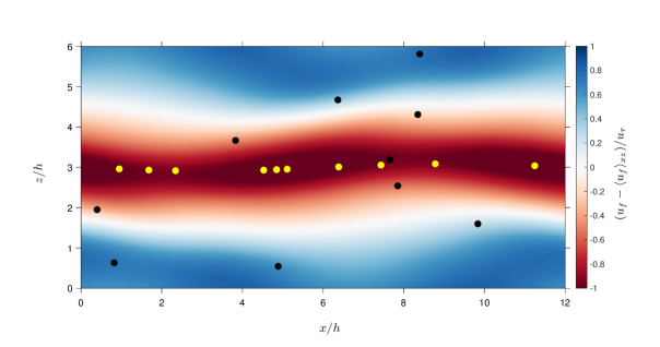
Figure 8: Same graph as in Fig. 6, but showing the initial positions (black circles) of the suspended particles in the multi-particle case M10, as well as the particle positions after an elapsed time of $120\,\tau_{b}$ (yellow circles).

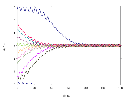
Figure 9: Spanwise particle position $z_{p}$ over time in bulk units for the multi-particle case M10. Each line corresponds to a different particle.

In order to check the dependency of our results upon the particle position at its time of release, we have simulated the temporal evolution starting from various initial values. For reasons of efficiency, we have done these tests in a multi-particle simulation (case M10 in Tab. 3), where 10 particles are simultaneously released at random positions in the wall-parallel plane in the vicinity of the lower wall (cf. Fig. 8). The evolution of the spanwise position, which is shown in Fig. 9, reveals that the spanwise motion in the asymptotic state is harmonic with the same period and amplitude for all particles. The latter matches well with the values found in the single-particle case S10, demonstrating two points: first, that particles migrate towards the low-speed streak irrespective of their initial position, and, second, that collective effects are not felt at this low particle concentration. Therefore, this multi-particle simulation confirms the observation that the persistent low-speed streak acts as a stable attractor to near-wall particle motion.

4.3 Constrained particles

While dynamical simulations (as the ones which we have presented above) can be used for the detection of stable equilibria of the system, it is not easy to find possible unstable equilibria with this method. Furthermore, it is of general interest to determine the stability properties of particle locations with respect to the coherent structures of the background flow in more detail. In order to obtain such additional information, it is useful to resort to the method of constrained simulations, where some otherwise dynamical quantity is held fixed, while the applied constraining force (or torque) is measured. This approach has been successfully used e.g. by Patankar et al. (2001) and by Joseph & Ocando (2002) for the investigation of the wall-normal migration of neutrally-buoyant particles in wall-bounded shear flows.

In the present context we proceed as follows. We seed the equilibrium solution with particles whose motion in the spanwise direction is suppressed, while they are free to move in the streamwise/wall-normal plane. We then let the simulation evolve until an asymptotic state is reached, which now features the particle translating on an essentially straight path (in the $x$-direction) in a time-periodic regime of motion, during which the hydrodynamic force acting upon the particles oscillates with the same period. The force component in the constraining direction at a given spanwise position, $F_{z}(z,t)$, is our primary quantity of interest. In case of a steady state system, the equilibria are then readily obtained as the positions $z_{e}$ where the force $F_{z}(z_{e})$ vanishes; stability (instability) can be detected by checking for negative (positive) gradients $\partial F_{z}/\partial z$ at the equilibrium positions. In the present case, where the constraining force is time-dependent, we perform the same analysis for the time-average of the spanwise component of the particle force, $\langle F_{z}(z,t)\rangle_{t}$. It should be noted that this is clearly a simplification, as the effect of temporal fluctuations upon the stability of the spanwise particle position are thereby effectively ignored. Therefore, this point might merit further investigation in future studies.

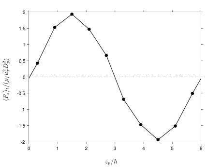
Figure 10: Time-average spanwise force for the last particle cycle in the constrained particle case C10, plotted as a function of the imposed spanwise position (i.e. one datum per particle).

In case C10 (with otherwise same parameters as cases S10 and M10, cf. Tab. 3) we perform a constrained simulation with 10 particles simultaneously (again for reasons of efficiency). In order to minimize their mutual influence, we initially place the particles uniformly on a diagonal in the $(x,z)$-plane. This numerical set-up was integrated in time for $116\,\tau_{b}$, which corresponds to more than 20 passages through the domain. However, we have verified that the forces acting on the particles already attain their asymptotic time evolution after only two of these passages, after which the values fluctuate by less than 5% from passage to passage. The time-average spanwise force $\langle F_{z}\rangle_{t}$ acting on the particles (in the asymptotic regime) is shown in Fig. 10 as a function of the respective spanwise position. As expected, the force exhibits two zero-crossings at $z_{e}/h=\{3,\,6\}$. One equilibrium position coincides with a positive gradient of the spanwise force ($z_{e}/h=6$), and it can therefore be classified as unstable; the other one ($z_{e}/h=3$), which coincides with the mean location of the low-speed streak, is stable, since the gradient of $\langle F_{z}\rangle_{t}$ is negative at that position.

Therefore, this simplified analysis confirms that the low-speed region is the only stable equilibrium for the particles’ spanwise location. Please note that this constrained simulation is significantly more efficient than the unconstrained one, since the transient time interval to be covered is much shorter. The present results consequently underline that the constrained simulation approach is a very useful tool in the context of computationally demanding resolved-particle DNS.

4.4 Density ratio

In order to elucidate the scaling of the particle mobility as a function of its inertia, we have varied the solid-to-fluid density ratio by a factor of twenty from case S04 to S80 (cf. Tab. 3), while maintaining all remaining physical and numerical parameters fixed (the Stokes and Galileo numbers vary accordingly). Please note that here we strictly separate the inertia effect from the geometrical size effect by keeping the particle diameter fixed. This is fundamentally different from varying the Stokes number in the context of a point-particle approach.

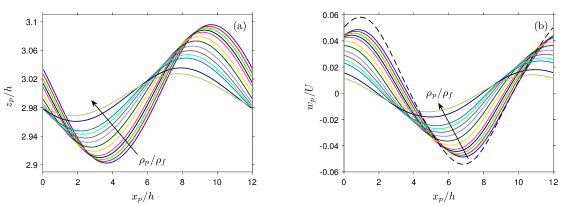
Figure 11: Single particle simulations at various solid/fluid density ratios. The data is for the asymptotic regime with fully-developed periodic particle motion. (a) Spanwise particle position as a function of the streamwise position. (b) Spanwise particle velocity as a function of the streamwise position. The color-code in both graphs refers to each run S04-S80 in Tab. 3, where the arrow indicates the direction of increase of $\rho_{p}/\rho_{f}$. The dashed curve in (b) shows the spanwise fluid velocity of the unperturbed flow field at the mean low-speed streak location and at a wall-distance equivalent to the particle’s centroid.

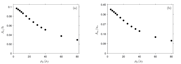
Figure 12: Amplitude of the spanwise particle motion (a) and the spanwise particle velocity (b) as a function of density ratio for cases S04-S80.

In all runs, the initial position of the particle is the same as in case S10, and the simulations are carried out for $110\,\tau_{b}$. After their initial release, all cases display similar dynamics as case S10 (as already shown in Fig. 7), and the time for the particles to reach the low-speed streak does not appear to depend significantly on the density ratio $\rho_{p}/\rho_{f}$ (figure omitted). Note that in all cases the particle remains in contact with the lower wall at all times, except for a short initial transient at the lowest Galileo number case S04. At later times, all runs exhibit a sinusoidal periodic motion in the $(x,z)$-plane, analogous to case S10, as can be seen from Fig. 11. In the asymptotic state, the particles oscillate around the same time-average position $\langle z_{p}\rangle_{t}/h=3$, irrespective of their density ratio. The amplitude and the phase of the particle motion, however, vary monotonously with $\rho_{p}/\rho_{f}$. More specifically, these amplitudes ($A_{z}$ for the spanwise particle excursions, and $A_{w}$ for the spanwise particle velocity fluctuations) are defined as one half of the difference between maximum and minimum values of the data shown in Figs. 11a and 11b, respectively. Fig. 12 then shows that over the investigated parameter range both amplitudes (spanwise particle position and velocity) first decrease roughly linearly with the density ratio, and then exhibit an increasingly non-linear evolution with $\rho_{p}/\rho_{f}$. This behavior can be qualitatively explained with the aid of very simple point-particle arguments, invoking Stokes drag to be the only particle force acting in the spanwise direction and assuming that the velocity seen by the particle is the unperturbed flow velocity of the equilibrium solution. Under these assumptions the amplitude of the spanwise particle excursions and of its spanwise velocity fluctuations decays as $(\rho_{p}/\rho_{f})^{-1}$ for large density ratios. However, in order to allow for a quantitative match with the data for finite-size particles, a more elaborate model would be required, taking into account unsteady force terms, finite-size and finite-Reynolds number corrections as well as wall effects. Again, the formulation of a realistic force model in the context of a point-particle approach would be a rewarding subject for future research, for which the present configuration can serve as a useful validation case.

5 Conclusions and perspectives for further studies

In this work we have attacked the problem of fluid-particle interaction with the aid of particle-resolved DNS based on an immersed-boundary method. Instead of considering turbulent flow and performing statistical analysis we have used a non-trivial equilibrium solution which features exact coherent structures (streaks and vortices) representative of the principal ingredients of wall-bounded shear flows. The present strategy has the advantage of a much reduced complexity, in particular in terms of ease of data-analysis.

More specifically, we have focused here on the upper branch of Nagata’s solution for plane Couette flow, which has previously been shown to reproduce some of the low-order statistics of the turbulent flow state. For the present work we have restricted our attention to a low Reynolds number, for which the single-phase flow solution is stable to finite-amplitude white noise perturbations. We have found that adding either a single or a small number of heavy spherical particles with a diameter equivalent to one twelfth of the gap width (2.5 wall units) does not significantly alter the flow structure, such that the background flow is essentially maintained. At the same time, a solid particle, which due to gravity remains in a plane adjacent to the lower horizontal wall, migrates towards the region occupied by a low-speed streak, and then attains a regime of periodic motion which is independent of the initial position. As a consequence of the particle’s preferential location, it does not sample the flow field uniformly, and, therefore, its time-average velocity differs from the (unperturbed) mean flow velocity at the wall-distance of its centroid.

This apparent velocity lag has previously been reported in experiments and in DNS studies of horizontal channel flow in the turbulent regime. Although past studies have already laid out the above mechanism leading to preferential particle concentration and its consequences, the data-analysis (involving coherent structure eduction and particle-conditioned statistical averaging) has required much effort. When using exact coherent structures as the background flow, this effort is significantly reduced. Furthermore, the technique of simulating constrained particles in order to determine the stability properties of particle motion can be applied to flow fields which are invariant solutions to the Navier-Stokes equations, as has been demonstrated in the present work.

Several new physical results have been obtained here by performing a sweep of the solid-to-fluid density ratio ($\rho_{p}/\rho_{f}=4\ldots 80$ corresponding to $St^{+}=1.4\ldots 27$). It turns out that the time it takes for the particle to migrate to the equilibrium position (inside the low-speed streak) does not significantly depend on the particle density in the range under investigation. In the asymptotic regime, on the other hand, the effect of particle inertia leads to the amplitude of the oscillations of the spanwise particle motion to decrease non-linearly with particle density.

To sum up, the present work demonstrates that it is technically feasible and beneficial to study invariant solutions (and in particular equilibrium solutions) with suspended finite-size particles. This set-up provides a numerical laboratory with minimal complexity, yet still relevant to the full problem of sustained turbulence. We expect the proposed approach to be fruitful in future studies on various aspects of particulate flow, and some perspectives for future work are briefly discussed in the following.

The most immediate avenue to pursue is to expand the study in parameter space. First, we note that in the present contribution we have not varied the particle diameter. It is obviously of interest to determine the limit for the occurrence of the preferential location mechanism as the particle size increases with respect to the scale of the coherent structures. Varying particle diameter and density independently will help to distinguish between relative size effects and inertial effects, as an alternative to the amalgamation of both in form of the Stokes number. Other important parameters which are straightforward to investigate in this framework include the role of gravity (sweep of Galileo number, orientation of the vector of gravitational acceleration), as well as an investigation of collective effects.

One important aspect which merits further analysis is the consideration of parameter points at which the equilibrium solution as such is already unstable (e.g. Nagata’s upper branch solution at larger Reynolds number). Preliminary computations indicate that the present approach still makes sense, as long as the solution remains suitably close to the equilibrium point over an interval which is long compared to the particle’s characteristic time scale. For some parameter points it is expected that the presence of particles adds to the de-stabilization of the flow. The study of the precise mechanisms by which particles contribute to the enhancement (or attenuation) of instability can be a rewarding subject by itself. Along these lines, we expect that the study of invariant solutions and finite-size particles can make a valuable contribution to the elucidation of open questions in the area of transition to turbulence in particulate flows (Matas et al., 2003; Loisel et al., 2013).

Since steady equilibrium solutions, such as the one considered herein, as well as other traveling-wave type solutions do not involve a notion of characteristic life-time of the coherent structures (i.e. the streaks and vortices are always present), possible effects of disparity of proper time scales in the fluid/particle interaction problem are not represented in this system. Therefore, it would be of great value to consider time-periodic invariant solutions (i.e. periodic orbits) in future studies involving solid particles. Prime candidates in this direction are the periodic solutions for plane Couette flow discovered by Kawahara & Kida (2001), which feature a self-sustaining cycle involving velocity-streak break-up and regeneration of quasi-streamwise vortices. At the present time, however, it is not clear whether it will be feasible to conduct numerical experiments involving finite-size particles suspended in such periodic orbit solutions.

Finally, let us mention that the present approach can obviously be extended to the study of small particles whose near-field does not need to be resolved (i.e. idealized as point particles). If the disperse phase is sufficiently dilute, the point-particle study can be conducted in one-way coupled fashion (i.e. the perturbation of the fluid phase can be neglected), which then renders the numerical simulations extremely efficient. Preliminary simulations of this type indicate that they will yield interesting information on preferential concentration and clustering. In addition, we see an opportunity to validate and eventually improve force models in the context of the point-particle approach with the aid of the present set-up. Such a study would have the clear advantage of full reproducibility. Further elaboration of this topic will be left for future work.

Appendix A Algorithm of the immersed boundary method

For each time step which advances the solution from $t^{n}$ to $t^{n+1}$ we perform three Runge-Kutta sub-steps with indices $\kappa=1,2,3$. The fractional step method first computes a pre-predicted velocity field $\tilde{\mathbf{u}}$ which does not include any explicit effect of the suspended particles. Next a force field $\mathbf{f}^{(ibm)}$ is computed which serves to impose the desired no-slip velocity at the particle surfaces. The momentum equations are then solved with the added force field to yield a predicted velocity field $\mathbf{u}^{\ast}$. Subsequently a Poisson equation is solved for the pseudo-pressure $\phi$ which then serves to project the velocity field upon the divergence-free space, yielding the final field $\mathbf{u}$. The particle equations of motion are finally updated to yield the new positions and particle velocities.

The overall algorithm for a single Runge-Kutta sub-step with index $\kappa$ can be written as follows:

$$\tilde{\mathbf{u}} = \mathbf{u}^{\kappa-1}+\Delta t\vphantom{\left.\mathbf{u}\right)^{\kappa-1}}2\alpha_{\kappa}\nu\nabla^{2}\mathbf{u}^{\kappa-1}-2\alpha_{\kappa}\nabla p^{\kappa-1}-\gamma_{\kappa}\left((\mathbf{u}\cdot\nabla)\mathbf{u}\right)^{\kappa-1}-\zeta_{\kappa}\left((\mathbf{u}\cdot\nabla)\mathbf{u}\right)^{\kappa-2}\,,$$ (9a)

$$\tilde{{U}}_{\beta}(\mathbf{X}_{l}^{(m)}) = \sum_{ijk}\tilde{{u}}_{\beta}(\mathbf{x}_{ijk}^{(\beta)})\,\delta_{h}(\mathbf{x}_{ijk}^{(\beta)}-\mathbf{X}_{l}^{(m)}(t^{\kappa-1}))\,\Delta x^{3}\,,\quad\forall\,l;\,m;\,\beta$$ (9b)

$$\mathbf{F}(\mathbf{X}_{l}^{(m)}) = \frac{\mathbf{U}^{(d)}(\mathbf{X}_{l}^{(m)},t^{\kappa-1})-\tilde{\mathbf{U}}(\mathbf{X}_{l}^{(m)},t^{\kappa-1})}{\Delta t}\,,\quad\qquad\qquad\forall\,l;\,m$$ (9c)

$${f}_{\beta}^{(ibm),\kappa}(\mathbf{x}_{ijk}^{(\beta)}) = \sum_{m=1}^{N_{p}}\sum_{l=1}^{N_{L}}{F}_{\beta}(\mathbf{X}_{l}^{(m)})\,\delta_{h}(\mathbf{x}_{ijk}^{(\beta)}-\mathbf{X}_{l}^{(m)}(t^{\kappa-1}))\,\Delta V_{l}^{(m)}\,,\quad\forall\,\beta;\,i;\,j;\,k$$ (9d)

$$\nabla^{2}\mathbf{u}^{\ast}-\frac{\mathbf{u}^{\ast}}{\alpha_{\kappa}\nu\Delta t} = -\frac{1}{\nu\alpha_{\kappa}}\left(\frac{\tilde{\mathbf{u}}}{\Delta t}+\mathbf{f}^{(ibm),\kappa}\right)+\nabla^{2}\mathbf{u}^{\kappa-1}\,,$$ (9e)

$$\nabla^{2}\phi = \frac{\nabla\cdot\mathbf{u}^{\ast}}{2\alpha_{\kappa}\Delta t}\,,$$ (9f)

$$\mathbf{u}^{\kappa} = \mathbf{u}^{\ast}-2\alpha_{\kappa}\Delta t\nabla\phi\,,$$ (9g)

$$p^{\kappa} = p^{\kappa-1}+\phi-\alpha_{\kappa}\Delta t\,\nu\nabla^{2}\phi\,,$$ (9h)

$$\frac{\mathbf{u}_{p}^{\kappa,\,(m)}-\mathbf{u}_{p}^{\kappa-1,\,(m)}}{\Delta t} = \frac{\rho_{f}}{V_{p}(\rho_{p}-\rho_{f})}\left(-{\mathcal{F}}^{\kappa,\,(m)}+\sum_{l\neq m}\mathbf{F}_{rep}^{\kappa-1,\,(l,m)}+\mathbf{F}_{wall}^{\kappa-1,\,(m)}\right)+2\alpha_{\kappa}\mathbf{g}\,,\qquad\forall\,m$$ (9i)

$$\frac{\mathbf{x}_{p}^{\kappa,\,(m)}-\mathbf{x}_{p}^{\kappa-1,\,(m)}}{\Delta t} = \alpha_{\kappa}\left(\mathbf{u}_{p}^{\kappa,\,(m)}+\mathbf{u}_{p}^{\kappa-1,\,(m)}\right)\,,\qquad\forall\,m$$ (9j)

$$\frac{\boldsymbol{\omega}_{p}^{\kappa,\,(m)}-\boldsymbol{\omega}_{p}^{\kappa-1,\,(m)}}{\Delta t} = -\frac{\rho_{f}}{\rho_{p}-\rho_{f}}\frac{1}{(I_{p}/\rho_{p})}\,{\mathcal{T}}^{\kappa,\,(m)}\,,\qquad\forall\,m$$ (9k)

where $m$ is the index of a given particle ($1\leq m\leq N_{p}$), $\beta$ denotes a spatial direction ($1\leq\beta\leq 3$), $\mathbf{X}_{l}^{(m)}$ is the position of a Lagrangian force point with index $l$ (where $1\leq l\leq N_{l}$) attached to the $m$th particle, $\delta_{h}$ is the discrete delta function of Roma et al. (1999), $\mathbf{x}_{ijk}^{(\beta)}$ is the position vector of a node of the staggered Cartesian fluid grid of the velocity component in the $x_{\beta}$ direction with index triplet “$ijk$”, $\tilde{{U}}_{\beta}$ is the velocity in the $x_{\beta}$-direction interpolated to a Lagrangian position, $\mathbf{U}^{(d)}(\mathbf{X}_{l})$ is the solid body velocity of the Lagrangian force point, $\mathbf{F}(\mathbf{X}_{l}^{(m)})$ is the immersed boundary force at a Lagrangian force point, $\Delta V_{l}^{(m)}$ is the forcing volume associated to the $l$th Lagrangian forcing point of the $m$th particle (equal to $\Delta x^{3}$ here), $\mathbf{x}_{p}^{\kappa,\,(m)}$ is the centroid position of the $m$th particle, ${\mathcal{F}}^{\kappa,\,(m)}$ is the hydrodynamic force computed from the sum of the immersed boundary contributions of the $m$th particle, ${\mathcal{T}}^{\kappa,\,(m)}$ is the analogous hydrodynamic torque contribution, $\mathbf{F}_{rep}^{\kappa-1,\,(l,m)}$ and $\mathbf{F}_{wall}^{\kappa-1,\,(m)}$ are the force contributions from particle-particle and particle-wall contact, respectively. The set of coefficients $\alpha_{k}$, $\gamma_{k}$, $\xi_{k}$ for a low-storage scheme leading to second-order temporal accuracy has been given in Rai & Moin (1991). Please refer to the original publication Uhlmann (2005) for more details on the algorithm.

Appendix B Stability analysis

The stable/unstable parameter points of the upper-branch of Nagata’s solutions for domains $\boldsymbol{\Omega}_{1}$ and $\boldsymbol{\Omega_{2}}$ were previously summarized in form of shaded areas in the $(Re,\mathcal{E}_{D})$ state-space diagram (Fig. 2). Here, we list the discrete $Re$ and $\mathcal{E}_{D}$ values for which the stability analysis was performed —  see Tab. 4.

In Tab. 4, the reader also finds the stable/unstable parameters points for a third domain, namely $\boldsymbol{\Omega}_{3}=[0,4\pi h]\times[-h,h]\times[0,2\pi h]$. Domain $\boldsymbol{\Omega}_{3}$ is identical to the one used in Clever & Busse (1997), where the authors conducted a linear stability analysis. The reproduction of their results served to validate our stability analysis approach, which is instead based on a time-stepper applied to an initial field which is perturbed by white noise, as detailed in Section 2.2.2. In all cases, we restrict our analysis to parameter points located on the upper-branch of Nagata’s solutions, as these are physically more interesting for the purpose of the current work.

Appendix C Computing single-phase equilibrium solutions with a finite-difference method

Here we wish to verify how closely the finite-difference solution on a given grid resembles the reference spectral results in the absence of particles. The equilibrium solution obtained with the Newton-Raphson approach and spectral-discretization is first spectrally interpolated upon the finite-difference grid, before starting time-stepping. Fig. 13 depicts the temporal evolution of kinetic energy for the stable parameter point (cf. Tab. 2) when using $384\times 128\times 192$ grid points, which implies a grid resolution of $(\Delta x^{+},\Delta y^{+},\Delta z^{+})=(0.50,0.25,0.50)$. The figure shows that the initial difference between $K^{fd}$ and $K^{ps}$ (i.e. the error due to spatial interpolation with a second-order method) is less than $0.01\,K^{ps}$. In Fig. 13 a mild temporal evolution in the form of a low-amplitude damped oscillation is subsequently observed for the finite-difference solution, which converges to within $0.7\%$ discrepancy of the spectral reference data.

Appendix D Grid convergence study for case S10

Here we compare the main findings of case S10 with results from case S10-F which features a refined grid. For this additional run, the number of grid points was increased by a factor of $3/2$ yielding $1152\times$$193\times 576$ nodes, i.e. $\Delta x^{+}=\Delta y^{+}=\Delta z^{+}=0.167$, and a particle resolution of $D_{p}/\Delta x=15$. The remaining numerical and physical parameters were held constant and are readily found in Tab. 3.

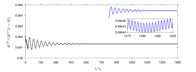
Figure 14: Time evolution of the box-averaged kinetic energy of the fluctuations $(K^{fd})$ in the baseline case S10 (  ) and after grid refinement, S10-F (  ). The inset shows a zoom over the last few cycles of the latter run.

The initial condition for case S10-F was taken from the state of the system in case S10 at $t=820.50\,\tau_{b}$. The respective velocity field was first interpolated on the finer grid and the simulation was subsequently continued until $t=1500\,\tau_{b}$. The interpolation introduced disturbances in the former steady flow-field and gave rise to a new transient, as evidenced by the discontinuity in the time evolution of box-averaged kinetic energy in case S10-F shown in Fig. 14. The transient behavior is, as before, marked by a damped oscillation, which decays in time and slowly approaches a periodic state. The time-average of $(K^{fd})$ differs by 0.3% of $K^{ps}(t=0)$ between the computations on the two grids. Despite the lengthy time integration, we observe that the well-defined periodic motion previously seen in Fig. 5b is not yet fully established in case S10-F (see the inset in Fig. 14), whereas the signature of the periodic motion is already clearly developed. Note that the remaining slow modulation at the end of the simulation S10-F has an amplitude of approximately 1.5 times the amplitude of the oscillations related to the flow-through of the particle. The period of the latter oscillations in case S10-F measures $T_{po}\approx 1.94\,\tau_{b}$ which is in close agreement with case S10 (cf. Fig. 5b); for the amplitude of the fluctuations we observe a discrepancy of approximately 7% between the two grids.

Concerning the spanwise particle motion in the asymptotic regime, we find a good agreement between the results obtained with the two grids (S10 and S10-F) for the particle position (Fig. 15a) and velocity (Fig. 15b). For both signals, case S10-F exhibits amplitudes that are lower by 11% than in case S10. The shapes of the curves, however, remain unaltered, and re-scaling the spanwise velocity of the finer case recovers the signal of the coarser run. This confirms the negligible phase-lag between the two curves in Fig. 15.

Table 1: Geometrical dimensions of the plane Couette numerical set-up used to compute Nagata’s equilibrium solutions. The half wall separation is given by $h$ and an illustration of the computational domain is shown in Fig. 1.

Domain ID	$\mathcal{L}_{x}/h$	$\mathcal{L}_{z}/h$	$\lambda_{x}/h$	$\lambda_{z}/h$
$\boldsymbol{\Omega}_{1}$	6	3	6	3
$\boldsymbol{\Omega}_{2}$	12	6	12	6

Table 2: Physical parameters of the stable equilibrium solution selected to study the interaction between finite-size particles and exact coherent structures.

Domain ID	$Re$	$Re_{\tau}$	$\mathcal{E}_{D}$	$\lambda_{x}/h$	$\lambda_{z}/h$	$\mathcal{L}_{x}/\delta_{\nu}$	$\mathcal{L}_{z}/\delta_{\nu}$
$\boldsymbol{\Omega}_{2}$	$132.25$	$15.87$	$1.90$	$12$	$6$	$190.38$	$95.19$

Table 3: Physical parameters of the runs with Nagata’s solution at $Re=132.25$ on the upper branch of $\boldsymbol{\Omega}_{2}$ seeded with single or multiple finite-size particles. The diameter of the particles is $D_{p}/h=0.156$ ($D_{p}^{+}=2.48$). The fluid phase is discretized with $768\times 128\times 384$ grid points and the particle resolution measures $D_{p}/\Delta x=10$ in all cases.

Run ID	# Particles	$\rho_{p}/\rho_{f}$	$St$	$St^{+}$	$Ga$	$T_{obs}/\tau_{b}$	Colormap
S04	$1$	$4$	$0.22$	$1.37$	$3.16$	$110$
S06	$1$	$6$	$0.33$	$2.05$	$4.08$	$110$
S08	$1$	$8$	$0.44$	$2.73$	$4.83$	$110$
S10	$1$	$10$	$0.56$	$3.41$	$5.48$	$1500$
S12	$1$	$12$	$0.67$	$4.10$	$6.06$	$110$
S16	$1$	$16$	$0.89$	$5.46$	$7.07$	$110$
S20	$1$	$20$	$1.11$	$6.83$	$7.96$	$110$
S25	$1$	$25$	$1.39$	$8.53$	$8.95$	$110$
S30	$1$	$30$	$1.67$	$10.24$	$9.84$	$110$
S35	$1$	$35$	$1.94$	$11.95$	$10.65$	$110$
S40	$1$	$40$	$2.22$	$13.66$	$11.41$	$110$
S60	$1$	$60$	$3.33$	$20.48$	$14.03$	$110$
S80	$1$	$80$	$4.44$	$27.31$	$16.23$	$110$
M10	$10$	$10$	$0.56$	$3.41$	$5.48$	$120$	N/A
C10	$10$	$10$	$0.56$	$3.41$	$5.48$	$116$	N/A

Table 4: Parameter points on the upper-branch of Nagata’s solution for which a stability analysis was performed.

$\boldsymbol{\Omega}_{1}$: $(\lambda_{x},\lambda_{z})=(6h,3h)$			$\boldsymbol{\Omega}_{2}$: $(\lambda_{x},\lambda_{z})=(12h,6h)$			$\boldsymbol{\Omega}_{3}$: $(\lambda_{x},\lambda_{z})=(4\pi h,2\pi h)$
$\mathcal{E}_{D}$	$Re$	Stable?	$\mathcal{E}_{D}$	$Re$	Stable?	$\mathcal{E}_{D}$	$Re$	Stable?
$1.85$	$171.46$	No	$1.86$	$130.00$	Yes	$1.83$	$130.05$	Yes
$1.90$	$172.28$	No	$1.89$	$131.40$	Yes	$1.86$	$131.04$	Yes
$1.94$	$173.58$	No	$1.90$	$132.25$	Yes	$1.88$	$132.25$	Yes
$1.97$	$174.72$	No	$1.92$	$133.19$	Yes	$1.90$	$133.38$	Yes
$2.01$	$176.84$	No	$1.93$	$134.22$	No	$1.93$	$135.43$	No
$2.04$	$178.49$	No	$1.95$	$135.33$	No	$1.94$	$136.59$	No
$2.06$	$180.31$	No	$1.96$	$136.52$	No	$1.96$	$137.83$	No
$2.19$	$190.62$	No	$1.98$	$137.78$	No	$1.97$	$139.15$	No
$2.27$	$199.32$	No				$1.99$	$140.54$	No
$2.35$	$209.56$	No

Figure 1: Plane Couette flow geometry illustrating the numerical set-up. The physical domain is assumed periodic in the streamwise $(x)$ and spanwise directions $(z)$, whereas the $y$-direction is bounded by two walls that move in opposite directions, each with speed $U$. When a solid-phase is present, it consists of finite-size spherical particles with diameter $D_{p}$ and density $\rho_{p}$. Gravity $\mathbf{g}$ acts in the negative $y$-direction.

(a)

(a)

(b)

(a)

(b)

(a)

(b)

(a)

(b)

(a)

(b)

Figure 15: Data over one cycle in the asymptotic regime in case S10 (  ) and using the refined grid of S10-F (  ) showing: (a) the spanwise particle position; (b) the spanwise particle velocity component. In (b), the blue open circles (  ) represent the data from case S10-F scaled by the ratio of the two amplitudes.

References

- Balachandar & Eaton (2010) Balachandar, S. & Eaton, J. 2010 Turbulent dispersed multiphase flow. Ann. Rev. Fluid Mech. 42, 111–133.
- Bech et al. (1995) Bech, K. H., Tillmark, N., Alfredsson, P. H. & Andersson, H. I. 1995 An investigation of turbulent plane couette flow at low Reynolds numbers. J. Fluid Mech. 286, 291–325.
- Bergougnoux et al. (2014) Bergougnoux, L., Bouchet, G., Lopez, D. & Guazzelli, É. 2014 The motion of solid spherical particles falling in a cellular flow field at low Stokes number. Physics of Fluids 26 (9), 093302.
- Chouippe & Uhlmann (2015) Chouippe, A. & Uhlmann, M. 2015 Forcing homogeneous turbulence in direct numerical simulation of particulate flow with interface resolution and gravity. Physics of Fluids 27 (12), 123301.
- Clever & Busse (1992) Clever, R. M. & Busse, F. H. 1992 Three-dimensional convection in a horizontal fluid layer subjected to a constant shear. Journal of Fluid Mechanics 234, 511.
- Clever & Busse (1997) Clever, R. M. & Busse, F. H. 1997 Tertiary and quaternary solutions for plane Couette flow. Journal of Fluid Mechanics 344, 137.
- Clift et al. (1978) Clift, R., Grace, J. & Weber, M. 1978 Bubbles, drops and particles. Academic Press.
- Ehrenstein & Koch (1991) Ehrenstein, U. & Koch, W. 1991 Three-dimensional wavelike equilibrium states in plane Poiseuille flow. Journal of Fluid Mechanics 228, 111.
- Faisst & Eckhardt (2003) Faisst, H. & Eckhardt, B. 2003 Traveling Waves in Pipe Flow. Physical Review Letters 91 (22), 224502.
- García-Villalba et al. (2012) García-Villalba, M., Kidanemariam, A. G. & Uhlmann, M. 2012 DNS of vertical plane channel flow with finite-size particles: Voronoi analysis, acceleration statistics and particle-conditioned averaging. International Journal of Multiphase Flow 46, 54–74.
- Gibson et al. (2009) Gibson, J., Halcrow, J. & Cvitanovic, P. 2009 Equilibrium and travelling-wave solutions of plane couette flow. J. Fluid Mech. 638, 243–266.
- Glowinski et al. (1999) Glowinski, R., Pan, T.-W., Hesla, T. & Joseph, D. 1999 A distributed Lagrange multiplier/fictitious domain method for particulate flows. International Journal of Multiphase Flow 25 (5), 755–794.
- Hetsroni & Rozenblit (1994) Hetsroni, G. & Rozenblit, R. 1994 Heat transfer to a liquid-solid mixture in a flume. International Journal of Multiphase Flow 20 (4), 671–689.
- Hunt et al. (1988) Hunt, J., Wray, A. & Moin, P. 1988 Eddies, streams, and convergence zones in turbulent flows. In Proceedings of the Summer Programm, pp. 193–208. (Center for Turbulence Research, Stanford).
- Jiménez et al. (2005) Jiménez, J., Kawahara, G., Simens, M. P., Nagata, M. & Shiba, M. 2005 Characterization of near-wall turbulence in terms of equilibrium and ”bursting” solutions. Physics of Fluids 17 (1), 015105.
- Jiménez & Pinelli (1999) Jiménez, J. & Pinelli, A. 1999 The autonomous cycle of near-wall turbulence. Journal of Fluid Mechanics 389, 335–359.
- Joseph & Ocando (2002) Joseph, D. & Ocando, D. 2002 Slip velocity and lift. J. Fluid Mech. 454, 263–286.
- Kaftori et al. (1995) Kaftori, D., Hetsroni, G. & Banerjee, S. 1995 Particle behavior in the turbulent boundary layer. II. Velocity and distribution profiles. Physics of Fluids 7 (5), 1107–1121.
- Kawahara & Kida (2001) Kawahara, G. & Kida, S. 2001 Periodic motion embedded in plane Couette turbulence: Regeneration cycle and burst. Journal of Fluid Mechanics 449, 291–300.
- Kawahara et al. (2012) Kawahara, G., Uhlmann, M. & van Veen, L. 2012 The Significance of Simple Invariant Solutions in Turbulent Flows. Annual Review of Fluid Mechanics 44 (1), 203–225.
- Keller (1977) Keller, H. B. 1977 Numerical Solution of bifurcation and nonlinear eigenvalue problems. In Applications of Bifurcation Theory, pp. 359–384. Academic Press.
- Kerswell (2005) Kerswell, R. 2005 Recent progress in understanding the transition to turbulence in a pipe. Nonlinearity 18, R17–R44.
- Kidanemariam et al. (2013) Kidanemariam, A. G., Chan-Braun, C., Doychev, T. & Uhlmann, M. 2013 Direct numerical simulation of horizontal open channel flow with finite-size, heavy particles at low solid volume fraction. New Journal of Physics 15 (2), 025031.
- Kim et al. (1987) Kim, J., Moin, P. & Moser, R. 1987 Turbulence statistics in fully developed channel flow at low Reynolds number. J. Fluid Mech. 177, 133–166.
- Loisel et al. (2013) Loisel, V., Abbas, M., Masbernat, O. & Climent, E. 2013 The effect of neutrally buoyant finite-size particles on channel flows in the laminar-turbulent transition regime. Phys. Fluids 25 (12), 123304.
- Matas et al. (2003) Matas, J.-P., Morris, J. & Guazzelli, E. 2003 Transition to turbulence in particulate pipe flow. Phys. Rev. Lett. 90 (1), 014501.
- Maxey (2002) Maxey, M. R. 2002 The motion of small spherical particles in a cellular flow field. Physics of Fluids 30 (7), 1915.
- Nagata (1990) Nagata, M. 1990 Three-dimensional finite-amplitude solutions in plane Couette flow: bifurcation from infinity. Journal of Fluid Mechanics 217, 519.
- Niño & Garcia (1996) Niño, Y. & Garcia, M. H. 1996 Experiments on particle—turbulence interactions in the near–wall region of an open channel flow: implications for sediment transport. Journal of Fluid Mechanics 326, 285.
- Okino et al. (2010) Okino, S., Nagata, M., Wedin, H. & Bottaro, A. 2010 A new nonlinear vortex state in square-duct flow. J. Fluid Mech. 657, 413–429.
- Pan & Banerjee (1997) Pan, Y. & Banerjee, S. 1997 Numerical investigation of the effects of large particles on wall-turbulence. Physics of Fluids 9 (12), 3786–3807.
- Patankar et al. (2001) Patankar, N., Huang, P., Ko, T. & Joseph, D. 2001 Lift-off of a single particle in Newtonian and viscoelastic fluids by direct numerical simulation. J. Fluid Mech. 438, 67–100.
- Rai & Moin (1991) Rai, M. & Moin, P. 1991 Direct simulation of turbulent flow using finite-difference schemes. J. Comput. Phys. 96, 15–53.
- Rashidi et al. (1990) Rashidi, M., Hetsroni, G. & Banerjee, S. 1990 Particle-turbulence interaction in a boundary layer. International Journal of Multiphase Flow 16 (6), 935–949.
- Reeks et al. (2006) Reeks, M. W., Fabbro, L. & Soldati, A. 2006 In Search of Random Uncorrelated Particle Motion (RUM) in a Simple Random Flow Field. In Volume 1: Symposia, Parts A and B, , vol. 2006, pp. 1755–1762. ASME.
- Roma et al. (1999) Roma, A., Peskin, C. & Berger, M. 1999 An adaptive version of the immersed boundary method. J. Comput. Phys. 153, 509–534.
- Uhlmann (2005) Uhlmann, M. 2005 An immersed boundary method with direct forcing for the simulation of particulate flows. Journal of Computational Physics 209 (2), 448–476.
- Uhlmann (2008) Uhlmann, M. 2008 Interface-resolved direct numerical simulation of vertical particulate channel flow in the turbulent regime. Physics of Fluids 20, 053305.
- Uhlmann & Doychev (2014) Uhlmann, M. & Doychev, T. 2014 Sedimentation of a dilute suspension of rigid spheres at intermediate Galileo numbers: the effect of clustering upon the particle motion. Journal of Fluid Mechanics 752, 310–348.
- Uhlmann et al. (2010) Uhlmann, M., Kawahara, G. & Pinelli, A. 2010 Travelling-waves consistent with turbulence-driven secondary flow in a square duct. Phys. Fluids 22 (8), 084102.
- van Veen (2019) van Veen, L. 2019 A Brief History of Simple Invariant Solutions in Turbulence. In Computational Modelling of Bifurcations and Instabilities in Fluid Dynamics, , vol. 50, pp. 217–231.
- Waleffe (1998) Waleffe, F. 1998 Three-Dimensional Coherent States in Plane Shear Flows. Physical Review Letters 81, 4140–4143.
- Waleffe (2001) Waleffe, F. 2001 Exact coherent structures in channel flow. Journal of Fluid Mechanics 435, 93–102.
- Waleffe (2003) Waleffe, F. 2003 Homotopy of exact coherent structures in plane shear flows. Phys. Fluids 15 (6), 1517–1534.
- Yung et al. (1989) Yung, B. P., Merry, H. & Bott, T. R. 1989 The role of turbulent bursts in particle re-entrainment in aqueous systems. Chemical Engineering Science 44 (4), 873–882.