A goal oriented error estimator and mesh adaptivity for sea ice simulations

Abstract

For the first time we introduce an error estimator for the numerical approximation of the equations describing the dynamics of sea ice. The idea of the estimator is to identify different error contributions coming from spatial and temporal discretization as well as from the splitting in time of the ice momentum equations from further parts of the coupled system. The novelty of the error estimator lies in the consideration of the splitting error, which turns out to be dominant with increasing mesh resolution. Errors are measured in user specified functional outputs like the total sea ice extent. The error estimator is based on the dual weighted residual method that asks for the solution of an additional dual problem for obtaining sensitivity information. Estimated errors can be used to validate the accuracy of the solution and, more relevant, to reduce the discretization error by guiding an adaptive algorithm that optimally balances the mesh size and the time step size to increase the efficiency of the simulation.

1 Introduction

We consider the viscous-plastic (VP) sea model, that was introduced by Hibler in 1979 and which is still one of the most widely used sea ice rheologies as detailed by Stroeve et. al. (2014). The model includes strong nonlinearities such that solving the sea ice dynamics at high resolutions is extremely costly and good solvers are under active research. Mostly, solutions to the VP model are approximated by iterating an elastic-viscous-plastic (EVP) modification of the model that was introduced by Hunke and Dukowicz (1997) and that allows for explicit sub-cycling. Alternatively the VP model is tackled directly with simple Picard iterations as described by Hibler (1979) or solved with Newton-like methods as described by Lemieux et. al. (2010) or  Mehlmann and Richter (2017b). All approaches are not satisfactory as they are extremely expensive and often are not able to give an accurate solution in reasonable computational time. It is therefore of utmost importance to reduce the complexity of the computations, e.g. by using coarse meshes and large time step sizes, as long as this does not deteriorate the accuracy assumptions.

We derive an error estimator that identifies the errors coming from spatial and temporal discretization. Furthermore, the error estimator allows for a localization of the error to each element and each time step such that local step sizes can be adjusted. This goal oriented error estimator for the viscous-plastic sea model is an extension of the dual weighted residual method that was introduced by Becker and Rannacher (2001). The aim of the estimator is to identify discretization errors $J(U)-J(U_{k,h})$ between the unknown exact solution $U$ and the numerical approximation $U_{k,h}$, where $k$ indicates the temporal and $h$ the spatial discretization parameter, in functionals $J(\cdot)$. These functionals can be any measures of interest, e.g. the average sea ice extent in a certain time span

$$J(U_{k,h})=\frac{1}{t_{2}-t_{1}}\int_{t_{1}}^{t_{2}}\int_{\Omega}A_{k,h}(x,y,t)\,\text{d}(x,y)\,\text{d}t.$$ (1)

We denote by $A_{k,h}$ the ice concentration (one component of the solution $U_{k,h}$ which will be introduced later), by $\Omega\subset\mathds{R}^{2}$ the spatial domain of interest and by $[t_{1},t_{2}]$ the time span of interest, e.g. the summer months. The error estimator will give approximations to $J(U)-J(U_{k,h})$ which can be attributed to a spatial error, a temporal error and to a splitting error - coming from partitioning the system into momentum equation and balance laws, which is the standard procedure in sea ice numerics, see Lemieux et. al. (2014). The estimation of errors in space and time for parabolic problems was discussed by Schmich and Rannacher (2012). For the first time, we extend the application to the VP model and additionally consider the splitting error. Lipscomb et. al. (2007) pointed out that decoupling the system in time can lead to a numerical unstable solution such that a small time step is required to achieve a stable approximation. Lemieux et. al. (2014) introduced an implicit-explicit time integration method (IMEX), which resolves this issues and allows the use of larger time steps. The error estimator will be able to predict the accuracy implications of this temporal splitting.

Furthermore, it provides information about the spatial and temporal convergence of the approximation of the solution. So far spatial convergence has been analyzed by Williams and Tremblay (2018), where a one dimensional test case has been studied. The authors observe that the simulated velocity field depends on the spatial resolution and found that the mean sea ice drift speed rises by 32% by increasing resolution from 40 km to 5 km. The temporal and spatial scaling properties of the mean deformation rate and the sea ice thickness are studied by Hutter et. al. (2018).

The dual weighted residual estimator by Becker and Rannacher (2001) relies on a variational formulation of the system of partial differential equations and has been introduced for the finite element method. Later on, the estimator has been extended to time dependent problems by using a relation between classical time stepping schemes like the Euler method and temporal Galerkin methods, see Schmich and Vexler (2008), which can be considered as finite elements in time. This similarity is also exploited in this work. The temporal Galerkin approach appears abstract, but it allows for a simple realization in the context of standard time stepping schemes like the backward Euler method and it is necessary in order to formulate the estimator.

Likewise, finite volume methods can be interpreted as discontinuous Galerkin methods that also give direct access to the framework of the dual weighted residual estimator, see Afif et. al. (2003) or Chen and Gunzburger (2014) for an approach that does not rely on this similarity to Galerkin methods and which shows applications in climate modeling. An application of the goal oriented error estimator in finite difference discretizations is less natural, since the variational structure is missing. This however is the basis for the definition of adjoint problems and also of the residual terms that form the estimator. However, low order finite elements are closely related to finite difference methods obtained by numerical quadrature. This similarity is used by Meidner and Richter (2015) to apply the error estimator to efficient finite difference time stepping schemes and Collins et. al. (2014) exploit the similarity of finite difference schemes with related finite volume and finite element formulations to carry over the idea of the error estimator to spatial finite difference discretizations of conservation laws.

The paper is structured as follows. In Section 2 we start by presenting the sea ice model in strong and variational formulation which is required for the Galerkin finite element discretization in space and time. Further we give details on the partitioned solution approach. In Section 3 we derive the goal oriented error estimator for the sea ice model and describe its numerical realization. We numerically analyse the error estimator in Section 4 and conclude in Section 5. For better readability we keep the mathematical formulation as simple as possible and refer to the literature for details. Some details on variational formulations are given in the appendix.

2 Model Description and Discretization

Let $\Omega\subset\mathds{R}^{2}$ be the spatial domain. We denote the time interval of interest by $I=[0,T]$. Sea ice is described by three variables, the sea ice concentration $A$, the mean sea ice thickness $H$ and the sea ice velocity $\mathbf{v}$, such that the complete solution is given by $U=(\mathbf{v},A,H)$. The VP sea ice model as introduced by Hibler (1979) consists of the momentum equation and the balance laws

$$\rho_{\text{ice}}H\big{(}\partial_{t}\mathbf{v}+f_{c}\vec{e}_{r}\times(\mathbf{v}-\mathbf{v}_{\text{ocean}})\big{)} =\operatorname{div}\,\boldsymbol{\sigma}+\boldsymbol{\tau}(\mathbf{v}),$$ (2)

$$\partial_{t}A+\operatorname{div}\,(\mathbf{v}A)=S_{A},\quad\partial_{t}H +\operatorname{div}\,(\mathbf{v}H)=S_{H}$$

with $0\leq H$ and $0\leq A\leq 1$. The forcing term $\boldsymbol{\tau}(\mathbf{v})$ models ocean and atmospheric traction

$$\boldsymbol{\tau}(\mathbf{v})=C_{\text{ocean}}\rho_{\text{ocean}}\|\mathbf{v}_{\text{ocean}}-\mathbf{v}\|_{2}(\mathbf{v}_{\text{ocean}}-\mathbf{v})+C_{\text{atm}}\rho_{\text{atm}}\|\mathbf{v}_{\text{atm}}\|_{2}\mathbf{v}_{\text{atm}},$$

with the ocean velocity $\mathbf{v}_{\text{ocean}}$ and the wind velocity $\mathbf{v}_{\text{atm}}$. By $\rho_{\text{ice}}$ we denote the ice density, by $f_{c}$ the Coriolis parameter, by $\vec{e}_{r}$ the radial ($z$-direction) unit vector. Following Coon (1980) we have replaced surface height effects by the approximation $g\nabla\tilde{H}_{g}=-f_{c}\vec{e}_{r}\times\mathbf{v}_{\text{ocean}}\approx 0$. In this paper we focus on the dynamical part of the sea ice model such that we neglect thermodynamic effects and set $S_{A}=0$ and $S_{H}=0$.

Parameter	Definition	Value
$\rho_{\text{ice}}$	sea ice density	$900\,\mathrm{kg/m^{3}}$
$\rho_{\text{atm}}$	air density	$1.3\,\mathrm{kg/m^{3}}$
$\rho_{\text{ocean}}$	water density	$1026\,\mathrm{kg/m^{3}}$
$C_{\text{atm}}$	air drag coefficient	$1.2\,\mathrm{\cdot}{10^{-3}}$
$C_{\text{ocean}}$	water drag coefficient	$5.5\,\mathrm{\cdot}{10^{-3}}$
$f_{c}$	Coriolis parameter	$1.46\,\mathrm{\cdot}10^{-4}\,\mathrm{s^{-1}}$
$P^{\star}$	ice strength parameter	$27.5\,\mathrm{\cdot}10^{3}\,\mathrm{N/m^{2}}$
$C$	ice concentration parameter	$20$

Table 1: Physical parameters of the momentum equation.

The system of equations (2) is closed by Dirichlet conditions $\mathbf{v}=0$ on the boundary of the domain and initial conditions $H(0)=H^{0}$, $A(0)=A^{0}$ and $\mathbf{v}(0)=\mathbf{v}^{0}$ for mean ice thickness, concentration and velocity at time $t=0$.

Finally, we present the nonlinear viscous-plastic rheology which relates the stress $\boldsymbol{\sigma}$ to the strain rate

$$\dot{\boldsymbol{\epsilon}}=\frac{1}{2}\Big{(}\nabla\mathbf{v}+\nabla\mathbf{v}^{T}\Big{)},\quad\dot{\boldsymbol{\epsilon}}^{\prime}:=\dot{\boldsymbol{\epsilon}}-\frac{1}{2}\operatorname{tr}(\dot{\boldsymbol{\epsilon}})I,$$

where $\operatorname{tr}(\cdot)$ is the trace. The rheology is given by

$$\boldsymbol{\sigma} =2\eta\dot{\boldsymbol{\epsilon}}^{\prime}+\zeta\operatorname{tr}(\dot{\boldsymbol{\epsilon}})I-\frac{P}{2}I,$$ (3)

with the viscosities $\eta$ and $\zeta$, given by $\eta=\frac{1}{4}\zeta$ and

$$\zeta=\frac{P}{2\Delta(\dot{\boldsymbol{\epsilon}})},\quad\Delta(\dot{\boldsymbol{\epsilon}}):=\sqrt{\frac{1}{2}\dot{\boldsymbol{\epsilon}}^{\prime}:\dot{\boldsymbol{\epsilon}}^{\prime}+\operatorname{tr}(\dot{\boldsymbol{\epsilon}})^{2}+\Delta_{min}^{2}}.$$ (4)

$\Delta_{min}=2\cdot 10^{-9}$ is the threshold that describes the transition between the viscous and the plastic regime. The ice strength $P$ in (3) is modeled as

$$P(H,A)=P^{\star}H\exp\big{(}-C(1-A)\big{)},$$ (5)

with the constant $C=20$. All problem parameters are collected in Table 1.

2.1 Variational formulation and discretization

The dual weighted residual estimator by Becker and Rannacher (2001) relies on a variational formulation of the system of partial differential equations in space and time and on Galerkin discretizations (like the finite element method) that discretize the problem by restricting the admissible space for finding the discrete solution. In our approach we use a linear finite element discretization in space and a discretization by piecewise constant functions in time, which also can be considered as a type of finite element discretization. This time discretization corresponds to the usual backward Euler method.

To start with, we multiply the three equations (2) with test functions $\boldsymbol{\phi}$, $\psi_{A}$ and $\psi_{H}$ and integrate in space and time

$$\int_{0}^{T}\Big{(}(\rho_{\text{ice}}H\partial_{t}\mathbf{v}+f_{c}\vec{e}_{r}\times\mathbf{v}-\rho_{\text{ice}}Hf_{c}\vec{e}_{r}\times\mathbf{v}_{\text{ocean}},\phi)\\ \quad+(\boldsymbol{\tau}(\mathbf{v}),\boldsymbol{\phi})+(\boldsymbol{\sigma},\nabla\boldsymbol{\phi})+(\partial_{t}A+\operatorname{div}\,(\mathbf{v}A),\psi_{A})\\ +(\partial_{t}H+\operatorname{div}\,(\mathbf{v}H),\psi_{H})\Big{)}\,\text{d}t=0.$$ (6)

By $(f,g)\coloneqq\int_{\Omega}f(x)g(x)\,\text{d}x$ we denote the usual $L^{2}$-inner product. Apart from the additional integration in time, this is the usual variational formulation for finite element discretizations as used in Danilov et. al. (2015).

In space, the discretization is briefly described: We define a conforming finite element space $V_{h}$ for velocity $\mathbf{v}\in V_{h}^{2}$, ice concentration and mean sea ice thickness $A,H\in V_{h}$. In our implementation we use the space of piecewise bi-linear functions defined on a quadrilateral mesh $\Omega_{h}$ of the domain $\Omega$. Danilov et. al. (2015), Dansereau et. al. (2016), Rampal et. al. (2016) consider finite element discretization on triangular meshes. The error estimator presented in the following section directly transfers to such discretizations, as it is shown in Carpio et. al. (2013).

To discretize (6) in time we split the interval $I=[0,T]$ into equidistant discrete steps $0=t_{0}<t_{1}<\cdots<t_{N}=T$ with $k\coloneqq t_{n}-t_{n-1}$. By discretizing with piecewise constant functions in time and by introducing appropriate scalar products that penalize the jumps of $\mathbf{v}$ and $H,A$ at each time step $t_{n}$ (compare Figure 6 in the Appendix for a visualization of the jumps), we obtain the standard implicit Euler discretization of the finite element formulation. For $n=1,2,\dots,N$ we solve

$$(\rho_{\text{ice}}H_{n}(\mathbf{v}_{n}-\mathbf{v}_{n-1}),\boldsymbol{\phi}_{h})+k(\rho_{\text{ice}}H_{n}f_{c}\vec{e}_{r}\times(\mathbf{v}_{n}-\mathbf{v}_{\text{ocean}}),\boldsymbol{\phi}_{h})$$ (7)

$$+k(\boldsymbol{\tau}(\mathbf{v}_{n}),\boldsymbol{\phi}_{h})+(\boldsymbol{\sigma}(\mathbf{v}_{n},A_{n},H_{n}),\nabla\boldsymbol{\phi}_{h}) =0$$

$$(A_{n}-A_{n-1},\psi_{A})+k(\operatorname{div}\,(\mathbf{v}_{n}A_{n}),\psi_{A}) =0$$

$$\qquad(H_{n}-H_{n-1},\psi_{H})+k(\operatorname{div}\,(\mathbf{v}_{n}H_{n}),\psi_{H}) =0$$

Division by the step size $k$ reveals the classical backward Euler scheme which is standard in sea ice dynamics as described by Lemieux et. al. (2014). The discrete functions $\mathbf{v}_{n},A_{n},H_{n},\boldsymbol{\phi}_{h},\psi_{A},\psi_{H}$ are all piecewise linear finite elements in space.

Remark 1

The transport equations for $A$ and $H$ are under the constraints $0\leq H$ and $0\leq A\leq 1$ which is not easily accessible for a variational formulation. We will therefore realize this constraint weakly by introduction of the following right hand side

$$(A_{n}-A_{n-1},\psi_{A})+k(\operatorname{div}\,(\mathbf{v}_{n}A_{n}),\psi_{A})=(\min\{0,1-A_{n}\},\psi_{A})$$

that only gets active if $A_{n}>1$ and that will then force $A_{n}$ below one.

To present the dual weighted residual error estimator we introduce the notation of the Galerkin formulation which is equivalent to the implicit Euler formulation given in (7)

$$\sum_{n=1}^{N}\int_{t_{n-1}}^{t_{n}}\Big{(}(\rho_{\text{ice}}H\big{(}\partial_{t}\mathbf{v}+f_{c}\vec{e}_{r}\times(\mathbf{v}-\mathbf{v}_{\text{ocean}})\big{)},\boldsymbol{\phi}_{h})\\ \quad\qquad+(\boldsymbol{\sigma}(\mathbf{v},A,H),\nabla\boldsymbol{\phi}_{h})+(\boldsymbol{\tau}(\mathbf{v}),\boldsymbol{\phi}_{h})\\ \quad\qquad+(\partial_{t}A+\operatorname{div}\,(\mathbf{v}A),\psi_{A})+(\partial_{t}H+\operatorname{div}\,(\mathbf{v}H),\psi_{H})\Big{)}\,\text{d}t\\ \qquad+(\rho_{\text{ice}}H(t_{n-1})^{+}[\mathbf{v}]_{n-1},\boldsymbol{\phi}(t_{n-1})^{+})\\ \qquad+([A]_{n-1},\psi_{A}(t_{n-1})^{+})+([H]_{n-1},\psi_{H}(t_{n-1})^{+})=0,$$ (8)

where the discrete function space, which contains piecewise constant functions in time and linear finite elements in space, is denoted by $V_{k,h}$. As the discrete functions of $V_{k,h}$ are discontinuous at each step $t_{n}$, we denote by $H(t_{n})^{+}$ and $H(t_{n})^{-}$ their values from the right and the left and by $[H]_{n}=H(t_{n})^{+}-H(t_{n})^{-}$ the jump of discontinuity. We also refer to Appendix A.1 for details and to Thomée (1997) for a comprehensive background on temporal Galerkin discretizations. The real solution is continuous in time and it holds $[\mathbf{v}]_{n}=0$ and $[A]_{n}=[H]_{n}=0$ such that the true solution to (2) or (6) is also a solution to this discrete formulation (8). The beauty of the Galerkin approach lies in the presence of one single problem formulation (8) that is equivalent to the original problem (2) if arbitrary functions are allowed for solution $\mathbf{v},\mathbf{h}$ and for testfunctions $\boldsymbol{\phi},\boldsymbol{\psi}$ and that is equivalent to the Euler / finite element discretization (7) if solution and test functions are restricted to piecewise constants in time and piecewise linear functions in space. We solve the problem with the established and efficient Euler scheme but we fall back to the Galerkin scheme in an integral formulation, when it comes to estimating the error, see Section 3.1.

To shorten notation we combine $U=(\mathbf{v},\mathbf{h})$ with $\mathbf{h}=(A,H)$ and $\Phi=(\boldsymbol{\phi},\boldsymbol{\psi})$ with $\boldsymbol{\psi}=(\psi_{A},\psi_{H})$ and we assume that these functions come from function spaces $U\in{\cal X}:={\cal V}\times{\cal V}^{A}\times{\cal V}^{H}$ and $\Phi\in{\cal X}$. The exact notation of all function spaces is introduced in Mehlmann and Richter (2017a). Then, the variational formulation (8) can written in an abstract notation by introducing the form $B(U)(\Phi)$ which simply collects all the integrals and jumps from (8)

$$U\in{\cal X}\quad B(U)(\Phi)=0\quad\forall\Phi\in{\cal X}.$$ (9)

The discrete solution $U_{k,h}=(\mathbf{v}_{k,h},A_{k,h},H_{k,h})\in X_{k,h}:=V_{k,h}\times V_{k,h}^{A}\times V_{k,h}^{H}$ is given by restricting (9) to the finite dimensional discrete space $X_{k,h}$

$$U_{k,h}\in X_{k,h}\quad B(U_{k,h})(\Phi_{k,h})=0\quad\forall\Phi_{k,h}\in X_{k,h}.$$ (10)

2.2 Partitioned solution approach

The discrete formulation (10) naturally splits into time-steps $t_{n-1}\to t_{n}$ as shown in (7). The three components velocity $\mathbf{v}$, ice concentration $A$ and mean ice thickness $H$ however are coupled. It is standard to apply a partitioned solution approach in every time step, either by first solving the momentum equation for the sea ice velocity followed by the balance laws, or vice versa, see Lemieux et. al. (2014). We first solve the momentum equation and replace all appearances of the ice concentration $A_{n}$ and mean ice thickness $H_{n}$ in the momentum equation of (7) by the previous approximations $H_{n-1}$ and $A_{n-1}$.

To realize this decoupling within the Galerkin formulation (8), we introduce the projection operator ${\cal S}:{\cal X}\to{\cal X}$ that projects $A\in{\cal V}^{A}$ (or $H$, respectively) on the interval $I_{n}=(t_{n-1},t_{n}]$ onto the value $H(t_{n-1})^{-}$. For discrete functions this corresponds to $S(H_{n})=H_{n-1}$ and $S(A_{n})=A_{n-1}$. This calls for a slight modification of the variational formulation $B(U)(\Phi)=0$ in (9), namely the introduction of the projection operator ${\cal S}$ in the momentum part

$$B_{s}(U)(\Phi)=\sum_{n=1}^{N}\int\limits_{t_{n-1}}^{t_{n}}\Big{(}(\rho_{\text{ice}}{\cal S}(H)\big{(}\partial_{t}\mathbf{v}+f_{c}\vec{e}_{r}\times(\mathbf{v}-\mathbf{v}_{\text{ocean}})\big{)},\boldsymbol{\phi}_{h})\\ \quad\qquad+(\boldsymbol{\sigma}(\mathbf{v},{\cal S}(A),{\cal S}(H)),\nabla\boldsymbol{\phi}_{h})+(\boldsymbol{\tau}(\mathbf{v}),\boldsymbol{\phi}_{h})\Big{)}\text{d}t\\ \qquad+(\rho_{\text{ice}}{\cal S}(H)(t_{n-1})^{+}[\mathbf{v}]_{n-1},\boldsymbol{\phi}(t_{n-1})^{+})+\dots{}$$ (11)

where the dots denote the equations for $A$ and $H$, which are not changed in comparison to (8). Once again, we indicate this variational form only for the formulation and evaluation of the error estimator, the solution itself is computed by the backward Euler scheme (7) by replacing $A_{n},H_{n}$ in the momentum equations by the previous approximations $A_{n-1},H_{n-1}$. Since the discretization is based on (11), but the exact solution is given by (8), the resulting discretization is called a non-consistent Galerkin formulation, see Appendix A.2 for details.

3 Goal oriented error estimation

In this section, we derive a goal oriented error estimator for partitioned solution approaches. The new error estimator will be based on concepts of the dual weighted residual (DWR) method introduced by Becker and Rannacher (2001). The DWR estimator can be easily applied to all problems given in a variational Galerkin formulation and it has been applied to various problems for error estimation in space and time such as fluid dynamics (Schmich and Rannacher (2012)) or fluid-structure interactions (Richter, 2017, Chapter 8).

The novel aspect of our approach is to properly include the error that stems from using a partitioned solution approach. Splitting will result in a non-consistent variational formulation, the analytical problem and the discrete problem do not match anymore. Measuring this splitting error will call for additional effort. This will be discussed in the following section and also in Appendix A.2. Further, in Section 4.2, we discuss the various parts that make up the error estimator. It will turn out that including this splitting error is essential as its share in the overall error can be dominant.

3.1 The goal oriented error estimator for partitioned solution approaches

The dual weighted residual estimator measures the discretization error with respect to a goal functional $J(\cdot)$ like (1), measuring the average sea ice extent. It is formulated as an optimization problem: we minimize $J(U)$ under the constraint that $U$ solves the sea ice problem. To tackle this optimization problem we introduce the Lagrangian

$$L(U,Z)\coloneqq J(U)-B(U)(Z),$$ (12)

where $Z$ takes the role of the Lagrange multiplier. Due to the splitting approach in time the discrete solution solves (11), but not (8). Thus, we introduce a second Lagrangian.

$$L_{s}(U_{k,h},Z_{k,h})\coloneqq J(U_{k,h})-B_{s}(U_{k,h})(Z_{k,h}),$$ (13)

which is based on the projection operator ${\cal S}$. This differentiates the error estimate from the standard dual weighted residual method, where it is sufficient to use only one Lagrangian.

Since $B(U)(Z)=0$ for the true solution and $B_{s}(U_{k,h})(Z_{k,h})=0$ for the discrete solution, we obtain the nonlinear error identity

$$J(U)-J(U_{k,h})=L(U,Z)-L_{s}(U_{k,h},Z_{k,h}),$$ (14)

We only sketch the derivation and refer to Mehlmann (2019) for details. The non-consistency of the variational formulation coming from the splitting approach is incorporated by introducing $\pm L(U_{k,h},Z_{k,h})=0$ and by separating the error influences into the Galerkin error (from discretization in space and time) and the splitting error (from partitioned time stepping)

$$J(U)-J(U_{k,h})=\underbrace{L(U,Z)-L(U_{k,h},Z_{k,h})}_{\text{Galerkin}}+\underbrace{L(U_{k,h})(Z_{k,h})-L_{s}(U_{k,h},Z_{k,h})}_{\text{splitting}}.$$

The estimation of the Galerkin part is the standard procedure of the dual weighted Galerkin method. We reformulate

$$L(U,Z)-L(U_{k,h},Z_{k,h})=\int_{0}^{1}\frac{d}{ds}L\big{(}U_{k,h}+s(U-U_{k,h}),Z_{k,h}+s(Z-Z_{k,h})\big{)}\,\text{d}s$$ (15)

and define the directional derivative of $L(U,Z)$ in an arbitrary direction $(\boldsymbol{\psi},\boldsymbol{\phi})$ as

$$L^{\prime}(U,Z)(\boldsymbol{\psi},\boldsymbol{\phi})\coloneqq\frac{d}{ds}L(U+s\boldsymbol{\psi},Z+s\boldsymbol{\phi})\Big{|}_{s=0}.$$ (16)

To shorten the notation we combine $X\coloneqq(U,Z)$ and $X_{k,h}\coloneqq(U_{k,h},Z_{k,h})$ and approximate the integral in (15) with the trapezoidal rule

$$L(U,Z)-L(U_{k,h},Z_{k,h})=L(X)-L(X_{k,h})\\ =\int_{0}^{1}L^{\prime}\big{(}X_{k,h}+s(X-X_{k,h})\big{)}\big{(}X-X_{k,h}\big{)}\,\text{d}s\\ =\frac{1}{2}L^{\prime}(X)(X-X_{k,h})+\frac{1}{2}L^{\prime}(X_{k,h})(X-X_{k,h})\\ +\frac{1}{2}\int_{0}^{1}s(1-s)L^{\prime\prime\prime}\big{(}X_{k,h}+s(X-X_{k,h})\big{)}\big{(}X-X_{k,h}\big{)}\,\text{d}s,$$ (17)

where we denote by $L^{\prime\prime\prime}(X)(\Psi)$ the third directional derivative of $L(X)=L(U,Z)$ in direction $\Psi$. See (Quarteroni et. al., 2007, Sec. 9.2.2) for a derivation of the trapecoidal rule’s error formula. The remainder is of third order in the error $X-X_{k,h}=(U-U_{k,h},Z-Z_{k,h})$ and omitted in practical application. If we consider the definition of the Lagrangian (12) the derivatives $L^{\prime}$ take the form

$$L^{\prime}(U,Z)(\delta U,\delta Z)=J^{\prime}(U)(\delta U)-B^{\prime}(U)(\delta U,Z)-B(U,\delta Z).$$

Details are given in Section 3.2. To proceed with the nonlinear error identity (17) we now define $Z\in{\cal X}$ as the solution to the linearized adjoint problem

$$B^{\prime}(U)(\Psi,Z) =J^{\prime}(U)(\Psi) \Psi \in{\cal X}$$ (18)

Analogously one differentiates $L_{s}^{\prime}$ and gets

$$B_{s}^{\prime}(U)(\Psi,Z) =J^{\prime}(U)(\Psi) \Psi \in{\cal X}$$ (19)

$$B_{s}^{\prime}(U_{k,h})(\Psi,Z_{k,h}) =J^{\prime}(U_{k,h})(\Psi) \Psi \in X_{k,h},$$

where we define $Z_{k,h}\in{\cal X}$ as the solution to discretized linearized adjoint problem.

Remark 2 (Adjoint solution)

The solution $Z$ to the linearized adjoint problem (18) indicates the sensitivity of the error functional $J(U)$ with respect to the variations in the solution $U$. The adjoint solution runs backward in time and the direction of transport is reversed. The use of adjoint solutions is standard in the area of constraint optimization problems, where the adjoint solution takes the role of the Lagrange multiplier. In sea ice models (in general in all parts of climate models), adjoint equations play an eminent role in variational data assimilation, which can be considered as gradient based calibration of the model with respect to measurement data. The adjoint problems required for the process of error estimation result from the same linearized equations, with the right hand side given by the goal functional $J(\cdot)$. Some climate models like MITgcm (see Marotzke et. al. (1999); Heimbach et. al. (2005)) or MRI.COM (see Toyoda et. al. (2019)) support adjoint equations for coupled ice, ocean and atmosphere simulation. This will simplify the realization of the error estimator in climate models.

Equation (17) still depends on the discretization errors $U-U_{k,h}$ and $Z-Z_{k,h}$ which are unknown. However, these errors can be replaced by interpolation errors $U-I_{k,h}U$ and $Z-I_{k,h}Z$ which can be approximated by local reconstructions. For details we refer to Appendix A.2, see also Remark 3.

The splitting part is derived by using the definitions of the Lagrangians in (12) and (13)

$$L(U_{k,h},Z_{k,h})-L_{s}(U_{k,h},Z_{k,h})=\beta(U_{k,h})(Z_{k,h}),$$ (20)

where the splitting error is given by the difference between original variational form (8) and splitting form (11)

$$\beta(U)(\Phi):=B_{s}(U)(\Phi)-B(U)(\Phi).$$ (21)

This error contribution can be evaluated since it only depends on quantities that are available, namely the primal and dual discrete solutions. We summarize:

Theorem 1 (DWR estimator for partitioned solution schemes)

Let $U,Z\in{\cal X}$ and $U_{k,h},X_{k,h}\in{\cal X}_{k,h}$ be primal and dual solutions to

$$B(U)(\Phi) =0 \forall\Phi \in{\cal X}$$

$$B^{\prime}(U)(\Psi,Z) =J^{\prime}(U)(\Psi) \forall\Psi \in{\cal X}$$

$$B_{s}(U_{k,h})(\Phi_{k,h}) =0 \forall\Phi_{k,h} \in X_{k,h}$$

$$B_{s}^{\prime}(U_{k,h})(\Psi_{k,h},Z_{k,h}) =J^{\prime}(U_{k,h})(\Psi_{k,h}) \forall\Psi_{k,h} \in X_{k,h}.$$

Then, it holds that

$$J(U)-J(U_{k,h})={\mathcal{R}}(x_{k,h},e)-\frac{1}{2}B_{s}(U_{k,h})(Z-I_{k,h}Z)\\ +\frac{1}{2}\Big{\{}J^{\prime}(U_{k,h})(U-I_{k,h}U)-B^{\prime}_{s}(U_{k,h})(U-I_{k,h}U,Z_{k,h})\Big{\}}\\ +\frac{1}{2}\Big{\{}\beta(U_{k})(Z+Z_{k})+\beta^{\prime}(U_{k})(U_{k},Z-Z_{k})\Big{\}}$$ (22)

where ${\mathcal{R}}(x_{k,h},e)$ is given in (17) and with the primal and dual splitting errors

$$\beta(U)(\Phi) :=B_{s}(U)(\Phi)-B(U)(\Phi),$$

$$\beta^{\prime}(U)(\Psi,Z) :=B_{s}^{\prime}(U)(\Psi,Z)-B^{\prime}(U)(\Psi,Z).$$

By $I_{k,h}:{\cal X}\to X_{k,h}$ we denote an interpolation to the space-time domain, by $U_{k}$ and $Z_{k}$ we denote semidiscrete solutions which are discretized in time only.

Remark 3 (Weights)

The error estimator (22) depends on the unknown solutions $U$ and $Z$ but also on semidiscrete solutions $U_{k}$ and $Z_{k}$, which are still continuous in space. All these terms must be approximated by suitable reconstruction techniques in order to evaluate the error estimator. In general, the reconstruction is realized by a postprocessing mechanism: The discrete solution is reinterpreted as a solution of double polynomial degree (linear in time instead of constant, quadratic in space instead of linear). In time, the discontinuity is resolved and in space we combine adjacent element to form the quadratic function. See Figure 7 in the appendix for an illustration of this reconstruction process. In time, we combine two intervals and reconstruct a linear function by connecting $U_{n-1}$ in $t_{n-1}$ with $U_{n}$ at $t_{n}$, i.e.

$$i_{k}^{(1)}U_{k,h}\Big{|}_{(t_{n-1},t_{n}]}=U_{n-1}+\frac{t-t_{n-1}}{k}(U_{n}-U_{n-1}).$$ (23)

Then, we approximate $U_{k}\approx i_{k}^{(1)}U_{k,h}$. In space a similar procedure is done by combining the piecewise linear function $U_{k,h}$ on four adjacent quadrilaterals to one quadratic function. We refer to Richter and Wick (2015) and Mehlmann (2019) for details. The notation $i_{k}^{(1)}$ means: interpolation to linear ($i^{(1)}$) functions on the same mesh $i_{k}$. Correspondingly, $i_{2h}^{(2)}$ stands for the interpolation to the space of quadratic functions $i^{(2)}$ on the space with double spatial mesh spacing $i_{(2h)}$.

3.1.1 Decomposing the error estimator

One application of the error estimator is to identify different contributions to the overall error, namely the error coming from discretization in space $\eta_{h}$, from the discretization in time $\eta_{k}$ and from the splitting $\eta_{\beta}$. This information can help to optimally balance the discretization, e.g. by avoiding excessive refinement (in space or time) or by avoiding (or by applying) a more costly implicit-explicit integration scheme (see Lemieux et. al. (2014)) to avoid the splitting error.

The structure of the error estimator (22) consists of residuals weighted by primal, $U-I_{k,h}U$, and dual, $Z-I_{k,h}Z$, interpolation errors and by two terms, $\beta$ and $\beta^{\prime}$, which measure the splitting error $\eta_{\beta}$. The residual primal and dual weighted residuals refer to the discretization error in space $\eta_{h}$ and in time $\eta_{k}$. An allocation of this combined space-time error can be achieved by introducing intermediate interpolations, which we discuss for the primal residual term $B_{s}(U_{k,h})(Z-I_{k,h}Z)$, the first term in (22). We introduce $\pm I_{k}Z$, an interpolation into the space of functions that are piecewise constant in time but still non-discrete in space

$$B_{s}(U_{k,h})(Z-I_{k,h}Z)=\underbrace{B_{s}(U_{k,h})(Z-I_{k}Z)}_{\text{time}}+\underbrace{B_{s}(U_{k,h})(I_{k}Z-I_{k,h}Z)}_{\text{space}}.$$ (24)

We can split the residual into two separate parts, as the dependency on the weight (which takes the role of the test function) is always linear.

Naturally, the interpolation $I_{k}Z$ is not available. However, we can approximate the interpolation errors by the reconstruction operator that have been mentioned in Remark 3. To be precise, the two terms in (24) are approximated by

$$B_{s}(U_{k,h})(Z-I_{k,h}Z)\approx B_{s}(U_{k,h})(i_{k}^{(1)}Z_{k,h}-Z_{k,h})+B_{s}(U_{k,h})(i_{2h}^{(2)}Z_{k,h}-Z_{k,h}).$$

The philosophy is simple: for estimating the error in time, we compare the discrete solution $Z_{k,h}$ with its higher order reconstruction in time $i_{k}^{(1)}Z_{k,h}$, the spatial error is estimated by considering the spatial reconstruction operator only. All further residual terms in (22) are handled in the same way.

3.2 Realization for sea ice dynamics

The standard feedback-approach for running adaptive simulations based on the DWR method is as follows:

Algorithm 1

Let $0=t_{0}<t_{1}<\cdots<t_{N}=T$ be the initial time mesh, $\Omega_{h}$ the initial spatial mesh. Let $V_{k,h}$ be the resulting space-time function space.

1. Solve the primal problem $U_{k,h}\in V_{k,h}$

2. Solve the dual problem $Z_{k,h}\in V_{k,h}$

3. Approximate the residual weights $U-I_{k,h}U$, $Z-I_{k,h}z$

4. Evaluate the error estimator (22)

5. Stop, if $|J(U)-J(U_{k,h})|$ is sufficiently small

6. Otherwise use the error estimator to adaptively refine the spatial and temporal discretization and restart with a finer function space ${\cal V}_{k^{\prime},h^{\prime}}$ on the refined mesh $\Omega_{h^{\prime}}$.

In Step 3, the approximation of the residual weights is the delicate part of the error estimator. Here, we must replace the unknown exact solutions $U$ and $Z$. For heuristic approaches we refer to Becker and Rannacher (2001), or in particular Schmich and Vexler (2008) or Meidner and Richter (2014) for time discretizations.

Application of the DWR method will always require some numerical overhead, mainly by the computation of the auxiliary dual problem. It turns out that the dual problem is always a linear problem, also in the case of the fully nonlinear sea ice problem. In the following sections we describe the steps that are required for applying the DWR estimator to the sea ice model in a partitioned solution framework. We refer to Mehlmann (2019) for the full derivation.

In order to apply the adaptive feedback loop presented in Algorithm 1, we will first indicate the exact discrete formulations for solving the primal and dual problems. These are not written as a discontinuous Galerkin formulation but in the form of the Euler method. Afterwards we give some further remarks on the evaluation of the error estimator.

Algorithm 2 (Primal sea ice problem)

Let $\mathbf{v}_{0}$ and $\mathbf{h}_{0}=(A_{0},H_{0})$ be the initial solutions at time $t=0$. Iterate for $n=1,...,N$

1. Solve for the velocity $\mathbf{v}_{n}\in V_{h}$

   $$k^{-1}(\rho_{\text{ice}}H_{n-1}(\mathbf{v}_{n}-\mathbf{v}_{n-1}),\phi)_{\Omega}\\ +(\rho_{\text{ice}}H_{n-1}f_{c}\vec{e}_{r}\times(\mathbf{v}_{n}-\mathbf{v}_{\text{ocean}})+\boldsymbol{\tau}(\mathbf{v}_{n}),\boldsymbol{\phi})_{\Omega}\\ +(\boldsymbol{\sigma}(\mathbf{v}_{n},H_{n-1},A_{n-1}),\nabla\boldsymbol{\phi})_{\Omega}=0\quad\forall\boldsymbol{\phi}\in V_{h}$$

2. Solve the transport equations for $A_{n}\in V^{A}_{h}$ and $H_{n}\in V^{H}_{h}$

   $$k^{-1}(A_{n}-A_{n-1},\psi_{A})_{\Omega}+(\operatorname{div}(\mathbf{v}_{n}A_{n}),\psi_{A})_{\Omega} =(\min\{0,1-A_{n}\},\psi_{A}) \quad\forall\psi_{A} \in V^{A}_{h},$$

   $$k^{-1}(H_{n}-H_{n-1},\psi_{H})_{\Omega}+(\operatorname{div}(\mathbf{v}_{n}H_{n}),\psi_{H})_{\Omega} =0\quad \forall\psi_{H} \in V^{H}_{h}$$

To derive the dual sea ice model defined in Theorem 1, we must differentiate the form $B_{s}(U)(\Phi)$, which is described in (11), in the direction of the solution $U=(\mathbf{v},\mathbf{h})$. The dual solution $Z=(\mathbf{w},\mathbf{q})$ replaces the test function and the new test function $\Psi=(\boldsymbol{\psi},\psi_{H},\psi_{A})$ is the argument of the directional derivative. The complete derivative of the variational formulation is presented in (Mehlmann, 2019, p. 131). For (rather) simple equations like the viscous plastic sea ice model it is most efficient to implement the dual solution (i.e. the adjoint of the linearization) analytically. The additional effort is minimal if a Newton scheme is employed for the solution of the forward problem since the adjoint system matrix is just the transposed of the Jacobian. In more complex coupled models and in particular, if variants of models are considered, the tangent problem (the Jacobian) and the adjoint can be efficiently generated by automatic differentiation, see Griewank and Walther (2008). This is approach is implemented in MITgcm, see Heimbach et. al. (2005).

Most characteristic for the dual problem is the reversal of the time direction, the problem runs backward in time. This reversal of direction also carries over to the splitting scheme. While the primal iteration first solves the momentum equation, the dual problem naturally results in first solving the (dual) transport problems, followed by the (dual) momentum equation.

Algorithm 3 (Partitioned solution approach for the dual system)

Let $\mathbf{v}_{n}$ and $\mathbf{h}_{n}$ for $n=0,\dots,N$, be the discrete solution of the primal problem. We set $\mathbf{v}_{N+1}:=0$ and $\mathbf{z}_{N+1}:=0$ and iterate backward in time from $n=N$ to $n=1$

1. Solve the dual transport equations for $\mathbf{q}_{n}=(\mathbf{q}_{A,n},\mathbf{q}_{H,n})\in V_{h}^{2}$

   $$k^{-1}(\mathbf{q}_{A,n}-\mathbf{q}_{A,n+1},\psi_{A})_{\Omega}-(\mathbf{v}_{n}\cdot\nabla\mathbf{q}_{A,n},\psi_{A})_{\Omega}\\ \qquad+\boldsymbol{\sigma}^{\prime}_{A}(\mathbf{v}_{n+1},H_{n},A_{n})(\psi_{A},\mathbf{z}_{n+1})=J^{\prime}_{A}(U_{n})(\psi_{A})-(\chi_{A_{n}>1},\psi_{A})_{\Omega}$$

   and

   $$k^{-1}(\mathbf{q}_{H,n}-\mathbf{q}_{H,n+1},\psi_{H})_{\Omega}-(\mathbf{v}_{n}\cdot\nabla\mathbf{q}_{H,n},\psi_{H})_{\Omega}\\ +(f_{c}\rho_{\text{ice}}\mathbf{z}_{n+1}\vec{e}_{r}\times(\mathbf{v}_{n+1}-\mathbf{v}_{\text{ocean}}(t_{n+1})),\psi_{H})_{\Omega}\\ +\boldsymbol{\sigma}^{\prime}_{A}(\mathbf{v}_{n+1},H_{n},A_{n})(\psi_{A},\mathbf{z}_{n+1})\\ +k^{-1}\rho_{\text{ice}}((\mathbf{v}_{n+1}-\mathbf{v}_{n})\mathbf{z}_{n+1},\psi_{H})=J^{\prime}_{H}(U_{n})(\psi_{H})$$

   for all $\psi_{A},\psi_{H}\in V_{h}$.

2. Solve the dual momentum equation for $\mathbf{z}_{n}\in V_{h}^{2}$

   $$k^{-1}(\rho_{\text{ice}}(H_{n-1}\mathbf{z}_{n}-H_{n}\mathbf{z}_{n+1}),\boldsymbol{\phi})_{\Omega}+(f_{c}\rho_{\text{ice}}H_{n-1}\vec{e}_{r}\times\boldsymbol{\phi},\mathbf{z}_{n})_{\Omega}\\ +(\boldsymbol{\tau}^{\prime}(\mathbf{v}_{n})(\boldsymbol{\phi}),\mathbf{z}_{n})_{\Omega}+(\boldsymbol{\sigma}^{\prime}_{\mathbf{v}}(\mathbf{v}_{n},H_{n-1},A_{n-1})(\boldsymbol{\phi},\mathbf{z}_{n}))_{\Omega}\\ -(H_{n}\nabla\mathbf{q}_{H,n},\boldsymbol{\phi})_{\Omega}-(A_{n}\nabla\mathbf{q}_{A,n},\boldsymbol{\phi})_{\Omega}=J^{\prime}_{\mathbf{v}}(U_{n})(\boldsymbol{\phi})$$

for all $\boldsymbol{\phi}\in V_{h}^{2}$. By $\chi_{A>1}(x)$ we denote the characteristic function satisfying $\chi_{A>1}(x)=1$ for $A(x)\geq 1$ and $\chi_{A>1}(x)=0$ for $A(x)<1$. By $\boldsymbol{\sigma}^{\prime}$ we denote the derivatives of the stress tensor with respect to $A$, $H$ or $\mathbf{v}$, by $\boldsymbol{\tau}^{\prime}$ the derivative of the forcing and by $J^{\prime}$ that of the functional. These terms are detailed in Mehlmann (2019).

Remark 4 (Dual problem)

The complexity of the dual system appears immense. However, the dual equation is linear such that the solution of each time step is very simple and comparable to one single Picard iterations of the forward problem, see Lemieux and Tremblay (2009).

If the sea ice system is linearized by a Newton method, it turns out that the dual system matrix is just the transposed of the Jacobian. It is hence not necessary to implement the rather complicated form of the equations in Algorithm 3. Instead, it is sufficient to assemble the Newton Jacobian and take its transpose.

Primal and dual problem in Algorithm 2 and 3 are given in the classical Euler time stepping formulation. To evaluate the error estimator (22) we must employ the equivalent variational formulations of the discrete forms (10) and (19), since the error estimator requires the testing with higher order reconstructions of the weights $i_{k}^{(1)}i_{2h}^{(2)}Z_{k,h}-Z_{k,h}$ and $i_{k}^{(1)}i_{2h}^{(2)}U_{k,h}-U_{k,h}$, compare Remark 3. Using the variational form is necessary since the equivalence to the Euler scheme only holds for piecewise constant trial and test functions but not for the reconstructed, piecewise linear weights. To approximate all integrals in (8) and the corresponding adjoint form with sufficient accuracy we employ the midpoint rule on each time step. To give an example: the forcing term $(\boldsymbol{\tau}(\mathbf{v}_{n}),\boldsymbol{\phi})_{\Omega}$ in Algorithm 2 corresponds to the space time integral $\int_{t_{n-1}}^{t_{n}}(\boldsymbol{\tau}(\mathbf{v}),\boldsymbol{\phi})\,\text{d}t$ in (8) and with the reconstructed weight $\boldsymbol{\phi}=i_{k}^{(1)}\mathbf{z}_{k,h}-\mathbf{z}_{k,h}$ the term within the error estimator is approximated by

$$(\mkern-4.0mu(\boldsymbol{\tau}(\mathbf{v}_{k,h}),i_{k}^{(1)}\mathbf{z}_{k,h}-\mathbf{z}_{k,h})\mkern-4.0mu)=\frac{k}{2}\sum_{n=1}^{N}\big{(}\boldsymbol{\tau}(\mathbf{v}_{n}),\big{(}\mathbf{z}_{n-1}-\mathbf{z}_{n}\big{)}\big{)}_{\Omega},$$

where we used that $i_{k}^{(1)}\mathbf{z}_{k,h}-\mathbf{z}_{k,h}=\frac{1}{2}(\mathbf{z}_{n-1}-\mathbf{z}_{n})$ in the midpoint of the interval $(t_{n-1},t_{n})$, compare Remark 3 and (23).

4 Numerical examples

Usually, a posteriori error estimators are used for two objectives: to compute an approximation with a certain accuracy as stopping criteria for the simulation, and, to adaptively control the discretization parameters, namely the mesh size and the time step size.

The first goal is not realistic in sea ice simulations. Uncertainties from measurement and from model inaccuracies are so large that quantitative error measures are not available. Furthermore, large scale simulations are computationally extremely challenging. Mostly there is little room for using finer and finer meshes. However, the described analysis of the different error contributions is of great computational importance as it allows to optimally balance all error contributions to avoid excessive over-refinement in space or in time. The estimator can help to steer the simulation such that a given error rate can be obtained with the smallest effort.

Fully adaptive simulations, possibly even using dynamic meshes that change from time step to time step, call for an enormous effort in terms of implementation that is usually only given in academic software codes (such as Gascoigne 3d, Becker et. al. (2019), which is used in this work). Global climate models do not offer this flexibility. However, some models like FESOM (Danilov et. al. (2015)), MPAS (Ringler et. al. (2013)) or ICON (Korn (2017)) offer the possibility for regional refinement in different zones. The error estimator can be used for automatically selecting the proper refinement level of all zones to reach the best accuracy on a discretization that is as coarse as possible.

We start by describing a benchmark problem that has been introduced by Mehlmann and Richter (2017b). While keeping the test case simple (e.g. square domain) it features typical characteristics in terms of the forcing and the parameters. Then, we present different numerical studies on the error estimator. First we test its accuracy and effectivity in terms of adaptive mesh control, then focusing on possible cases for an integration of such techniques in climate models.

4.1 Definition of a benchmark problem

For all test cases we consider the domain $\Omega=(0,500\mathrm{km})^{2}$. At initial time $t=0$, the ice is at rest, $\mathbf{v}_{0}=0$, the ice concentration is constant $A=1.0$ and the ice height is a spatial variation around a thickness of $H=0.3\,\mathrm{m}$.

$$H^{0}(x,y)=0.3\,\mathrm{m}+0.005\,\mathrm{m}\left(\cos\left(\frac{x}{25\,\mathrm{km}}\right)+\cos\left(\frac{y}{50\,\mathrm{km}}\right)\right).$$

A circular steady ocean current is described by

$$\mathbf{v}_{\text{ocean}}(x,y)=0.01\,\mathrm{m\cdot s^{-1}}\begin{pmatrix}y/250\,\mathrm{km}-1\\ 1-x/250\,\mathrm{km}\end{pmatrix}.$$

The wind field mimics a cyclone and anticyclone that is diagonally passing through the computational domain going back and forth

$$v_{\text{atm}}(x,y,t)=15\,\mathrm{m\,s^{-1}}\omega(x,y)R(\alpha)\begin{pmatrix}x-m_{x}(t)\\ y-m_{y}(t)\end{pmatrix},$$

with the rotation matrix

$$R(\alpha):=\begin{pmatrix}\cos(\alpha)&\sin(\alpha)\\ -\sin(\alpha)&\cos(\alpha)\end{pmatrix}.$$

At initial time, the center of the cyclone is at $m_{x}(0)=m_{y}(0)=250\,\mathrm{km}$ and in $t\in[0,4\,\mathrm{days}]$ is moves to $m_{x}(4)=m_{y}(4)=450\,\mathrm{km}$ at constant speed. Then for $t\in[4\,\mathrm{days},12\,\mathrm{days}]$ it goes back to $m_{x}(12)=m_{y}(12)=50\,\mathrm{km}$ where it turns again towards $m_{x}(20)=m_{y}(20)=450\,\mathrm{km}$, and so on. When the direction is towards the upper left, the convergence angle is set to $\alpha=90^{\circ}-18^{\circ}$ and when it goes back towards the lower left we use $\alpha=90^{\circ}-9^{\circ}$. To reduce the wind strength away from the center, we choose $\omega(x,y)$ as

$$\omega(x,y) =\frac{1}{50}\exp\left(-\frac{r(x,y)}{100\,\mathrm{km}}\right),$$

$$r(x,y) =\sqrt{(x-m_{x}(t))^{2}+(y-m_{y}(t))^{2}}.$$

As functional of interest, we evaluate the average sea ice extent within a subset $\Omega_{2}\subset\Omega$ of the domain

$$\frac{1}{T}J_{A}(A)=\int_{0}^{T}\int_{\Omega_{2}}A(x,y,t)\,d(x,y)\,dt.$$ (25)

We specify $\Omega_{2}$ for each test case. Similar measures are considered for sea ice model evaluations or model intercomparisons, see Stroeve et. al. (2014) or Kwok and Rothrock (2009). The exact choice of the subdomain $\Omega_{2}$ and also the time interval of interest $I=[0,T]$ will be specified in the different test cases.

Solution of the nonlinear and linear systems

The nonlinear problems resulting in each time step of the forward simulation are solved with a modified Newton scheme that is described in Mehlmann and Richter (2017b). The linear systems within the Newton iteration and the linear problems of the dual system are solved with a GMRES method, preconditioned by a geometric multigrid solver as introduced in Mehlmann and Richter (2017a). The model is implemented in the software library Gascoigne 3d, see Becker et. al. (2019).

4.2 Sharpness of the error estimate

In a first test case we evaluate the sharpness of the error estimator, i.e. its capability of predicting an quantitatively exact error value. As noted in the introduction to this section, this scenario may not be of highest use in applications. However, it is an important test case for the validation of the estimator itself. For this first test case we use the short time interval $I=[0,1\,\mathrm{day}]$ and the subdomain for measuring the functional $\Omega_{2}=(375\,\mathrm{km},500\,\mathrm{km})^{2}\subset\Omega$. On a fine mesh with $h_{ref}=1\,\mathrm{km}$ and with the time step size $k_{ref}=0.125\,\mathrm{h}$ we obtain the value

$$\tilde{J}_{A}:=J_{A}(U_{k_{ref},h_{ref}})=1.49907\pm 10^{-5},$$ (26)

in reference units, which corresponds to the average sea ice extent of 15615$\text{km}^{2}$. We will take $\tilde{J}_{A}$ as reference value for the following computations.

$h$	$k$	$J_{A}(U^{s}_{k,h})$	$\tilde{J}_{A}-J_{A}(U^{s}_{k,h})$	$\eta_{k,h}$	$\eta_{h}$	$\eta_{k}$	$\eta_{\beta}$
64 km	8 h	1.49763	1.44$\cdot 10^{-3}$	2.01$\cdot 10^{-3}$	1.20$\cdot 10^{-3}$	2.65$\cdot 10^{-3}$	1.58$\cdot 10^{-4}$
32 km	8 h	1.49788	1.19$\cdot 10^{-3}$	1.38$\cdot 10^{-3}$	1.21$\cdot 10^{-4}$	2.19$\cdot 10^{-3}$	4.40$\cdot 10^{-4}$
16 km	8 h	1.49797	1.10$\cdot 10^{-3}$	1.30$\cdot 10^{-3}$	6.72$\cdot 10^{-5}$	2.10$\cdot 10^{-3}$	4.38$\cdot 10^{-4}$
8 km	8 h	1.49802	1.05$\cdot 10^{-3}$	1.25$\cdot 10^{-3}$	4.11$\cdot 10^{-5}$	2.03$\cdot 10^{-3}$	4.21$\cdot 10^{-4}$
64 km	4 h	1.49833	7.43$\cdot 10^{-4}$	9.52$\cdot 10^{-4}$	6.28$\cdot 10^{-4}$	1.21$\cdot 10^{-3}$	6.12$\cdot 10^{-5}$
32 km	4 h	1.49849	5.80$\cdot 10^{-4}$	6.16$\cdot 10^{-4}$	8.53$\cdot 10^{-5}$	1.02$\cdot 10^{-3}$	1.25$\cdot 10^{-4}$
16 km	4 h	1.49856	5.15$\cdot 10^{-4}$	5.72$\cdot 10^{-4}$	4.41$\cdot 10^{-5}$	9.70$\cdot 10^{-4}$	1.30$\cdot 10^{-4}$
8 km	4 h	1.49858	4.87$\cdot 10^{-4}$	5.51$\cdot 10^{-4}$	2.47$\cdot 10^{-5}$	9.44$\cdot 10^{-4}$	1.32$\cdot 10^{-4}$
64 km	2 h	1.49863	4.39$\cdot 10^{-4}$	5.67$\cdot 10^{-4}$	5.48$\cdot 10^{-4}$	5.67$\cdot 10^{-4}$	2.04$\cdot 10^{-5}$
32 km	2 h	1.49876	3.10$\cdot 10^{-4}$	2.94$\cdot 10^{-4}$	7.01$\cdot 10^{-5}$	4.82$\cdot 10^{-4}$	3.67$\cdot 10^{-5}$
16 km	2 h	1.49881	2.59$\cdot 10^{-4}$	2.67$\cdot 10^{-4}$	3.58$\cdot 10^{-5}$	4.59$\cdot 10^{-4}$	3.95$\cdot 10^{-5}$
8 km	2 h	1.49883	2.37$\cdot 10^{-4}$	2.54$\cdot 10^{-4}$	1.93$\cdot 10^{-5}$	4.47$\cdot 10^{-4}$	4.19$\cdot 10^{-5}$

Table 2: On a sequence of spatially and temporally refined meshes we compare the functional output $J_{A}(U_{k,h}^{s})$ to the reference value $\tilde{J}_{A}\approx 1.49907$ and indicate the error $\tilde{J}_{A}-J_{A}(U_{k,h}^{s})$, the total error estimator $\eta_{k,h}=\frac{1}{2}(\eta_{h}+\eta_{k}+\eta_{\beta})$ and its contributions attributing the spatial discretization error $\eta_{h}$, the temporal discretization error $\eta_{k}$ and the splitting error $\eta_{\beta}$. We observe that the complete error estimate $\eta_{k,h}$ is very close to the real error and that the temporal error is dominating on fine spatial meshes. On the right, we show the composition of the error estimator into spatial error $\eta_{h}$, temporal error $\eta_{k}$ and splitting error $\eta_{\beta}$ for a fixed spatial mesh and varying time step sizes (top) and for a fixed temporal mesh and varying spatial mesh sizes (bottom).

Figure 1: Effectivity index $\text{eff}_{k,h}$ of the error estimator for different temporal and spatial discretizations. The estimator is highly accurate with only about $20\%$ of overestimation.

In Table 2, we evaluate the functional error $|\tilde{J}_{A}-J_{A}(U^{s}_{k,h})|$ and the error estimator given by (22), which we denote by $\eta_{k,h}$. In the plots on the right side of Table 2, we show the composition of the error estimator into spatial error, temporal error and splitting error. The upper figure shows that, for a fixed spatial mesh with $h=16$km, linear convergence is obtained for $\eta_{k}$ and $\eta_{\beta}$ under temporal refinement, whereas the spatial error naturally stagnates. The lower figure shows in a similar fashion that, for a fixed time mesh with $k=2$h, spatial refinement results in linear convergence in space, whereas temporal error and splitting error do not get smaller. This clear decomposition of the error estimator into spatial and temporal contributions will allow us to design an adaptive algorithm that efficiently controls the discretization in order to balance temporal and spatial error, see Section 4.3. Overall, this example shows a dominance of the temporal error, which is due to the short simulation time of $1$ day, where nearly no kinematic features appear. To validate the accuracy of the error estimator we introduce the effectivity index

$$\text{eff}_{k,h}:=\frac{\tilde{J}_{A}-J(U^{s}_{k,h})}{\eta_{k,h}},$$ (27)

which measures the sharpness of the estimate. If this index is close to one, true error and estimator are very close $\eta_{k,h}\approx\tilde{J}_{A}-J(U^{s}_{k,h})$ such that the estimate is very accurate. If the index is much larger than one, the estimator overestimates the true error, if it is much smaller than one, the estimator underestimates the error. In Figure 1, we plot this effectivity index and find $0.75\leq\text{eff}_{k,h}\leq 1.1$ which indicates that the error estimator is highly accurate, in particular for increasing spatial and temporal resolutions.

The last three columns of Table 2 show the decomposition of the error estimator into spatial, temporal and splitting part as described in Section 3.1.1. These values show a dominance of the temporal error over the spatial error and to lesser degree also over the splitting error. In space, the estimator values $\eta_{h}$ also clearly demonstrate linear convergence in $h$, which is expected for linear finite elements. We do not observe this convergence order in the overall error, as it is dominated by the other two parts. The second test case in Section 4.4 shows a dominance of the spatial error. The dominating temporal residual error stems from the short simulation time of $T=1\,\mathrm{day}$. Our findings coincide with the analysis of Lemieux et. al. (2014) where the temporal error also dominates the splitting error in a one day simulation. A test case running for $33\,\mathrm{days}$ discussed in Section 4.4 shows a balanced distribution of spatial and temporal errors.

4.3 Balancing error contributions

A simple application of the decomposition of the error estimator into spatial error, temporal error and splitting error is to balance the different error contributions by the following algorithm:

Algorithm 4 (Balancing errors)

Given an initial time step size $k$ and mesh size $h$. Iterate:

1. Solve the sea ice problem $u_{k,h}\in V_{k,h}$

2. Estimate the error according to Algorithm 1

3. Split the error estimate $\eta_{k,h}:=\frac{1}{2}(\eta_{h}+\eta_{k}+\eta_{\beta})$

4. If $\eta_{k}+\eta_{\beta}>2\eta_{h}$ refine time step $k\mapsto\frac{k}{2}$
   If $\eta_{h}>2(\eta_{k}+\eta_{\beta})$ refine spatial mesh $h\mapsto\frac{h}{2}$
   Otherwise refine in space and time $k,h\mapsto\frac{k}{2},\frac{h}{2}$
   

Here, we have attributed the splitting error $\eta_{\beta}$ to the temporal error. We refine only spatially (or temporally) if this error contribution is twice as large as the other part. If the errors are already close to each other, we refine in space and in time. This strategy can be extended to include further error contributions. In coupled ice-ocean simulations one could balance the errors of the ocean component and the ice component.

We virtually perform a simulation based on Algorithm 4 by processing the results from Table 2. Starting with $h=64\,\mathrm{km}$ and $k=8\,\mathrm{h}$ it holds $\eta_{k}+\eta_{\beta}=2.71\cdot 10^{-3}>2\eta_{h}=2.40\cdot 10^{-3}$ (compare the first line of Table 2). Hence, we refine in time only and proceed with $h=64\,\mathrm{km}$ and $k=4\,\mathrm{h}$. Again, it holds $\eta_{k}+\eta_{\beta}=1.27\cdot 10^{-3}>2\eta_{h}=1.26\cdot 10^{-3}$ such that we once more refine in time only, resulting in $h=64\,\mathrm{km}$ and $k=2\,\mathrm{h}$. This third simulation yields $\eta_{k}+\eta_{\beta}=5.87\cdot 10^{-4}\approx\eta_{h}=5.48\cdot 10^{-4}$ and we would continue by refining both in time and space.

Figure 2: Solution at day 15. On the left a uniform mesh with horizontal spacing $2\,\mathrm{km}$ and on the right an adaptive mesh using non-uniform mesh spacing between $64\,\mathrm{km}$ up to $2\,\mathrm{km}$ is used. The highlighted area is the domain $\Omega_{2}$ where we measure the average sea ice extent.

The natural alternative to this procedure would be a uniform refinement in space and in time whenever the accuracy is not sufficient. To compare the complexity of both approaches we assume that the algorithm scales optimally, i.e. linear in the number of time steps ${\cal O}(k^{-1})$ and linear in the number of mesh elements given by ${\cal O}(h^{-2})$.Altogether we use the simple model $E(k,h)=Ck^{-1}h^{-2}$ to measure the effort of one simulation. For simplicity, the constant is set to $C=64^{2}\cdot 8$. Three steps of uniform refinement result in the effort

$$E(8,64)+E(4,32)+E(2,16)=32\,768\Big{(}\frac{1}{64^{2}\cdot 8}+\frac{1}{32^{2}\cdot 4}+\frac{1}{16^{2}\cdot 2}\Big{)}=73$$

whereas the balancing algorithm yields

$$E(8,64)+E(4,64)+E(2,64)=32\,768\Big{(}\frac{1}{64^{2}\cdot 8}+\frac{1}{64^{2}\cdot 4}+\frac{1}{64^{2}\cdot 2}\Big{)}=7,$$

which is only $10\%$ of the effort for the uniform standard approach. On the final mesh, the balancing algorithm yields the error $4.39\cdot 10^{-4}$ compared to $2.59\cdot 10^{-4}$ that would be obtained by using uniform refinement in space and time (at 10 times the cost).

4.4 Adaptive mesh control and steering of regional refinement

In a second test case we consider a longer time horizon of $T=33\,\mathrm{days}$ and an initial sea ice concentration of $A=0.9$. The wind field described in Section 4.1 passes the domain several times and typical kinematic features appear. Figure 2 shows the sea ice ice concentration at day 15. The left figure gives a result on a uniform discretization, whereas the right plot belongs to the corresponding result on a locally refined mesh with about 3 times less unknowns. The highlighted quadrilateral area is the domain $\Omega_{2}=(250\,\mathrm{km},375\,\mathrm{km})^{2}$ where we evaluate the average sea ice extent

$$J(A)=\frac{1}{33\,\mathrm{days}}\int_{0}^{33\,\mathrm{days}}\int_{\Omega_{2}}A(x,t)\,\text{d}{x}\,\text{d}t.$$ (28)

Figure 3: Zoom into the adaptive mesh in the area of interest.

We focus on the spatial convergence and use the step size $k=0.5\,\mathrm{h}$ for all tests. We consider the contribution of the spatial discretization error $\eta_{h}$ only and use Algorithm 1 for identifying optimal finite element meshes to yield small errors on meshes that are as coarse as possible. Two different strategies are investigated. First, we use a fully local adaptive mesh concept, where mesh elements $K\in\Omega_{h}$ are refined into four smaller quadrilaterals, if the local error contribution $\eta_{K}$ is larger than the average error, i.e.

$$\eta_{K}>\gamma\cdot\bar{\eta}\quad\Rightarrow\quad\text{refine }K,\quad\bar{\eta}\coloneqq\frac{1}{|\Omega_{h}|}\sum_{K^{\prime}\in\Omega_{h}}\eta_{K^{\prime}}$$ (29)

where $\gamma\approx 1$ is a constant to fine-tune the refinement procedure. Usually we take $\gamma=2$. The results are shown in Figure 3. We focus on a small region around the area of interest $\Omega_{2}$ to better highlight the mesh that has been generated by the error estimator. It is not necessary to resolve the complete region of interest $\Omega_{2}$. Instead, parts outside of this region also have to be resolved to get the correct transport of information. Further, the resulting meshes appear rather tattered and non-symmetric. It is a typical feature of the error estimator that the resulting meshes are rather non-intuitive. We refer also to Becker and Rannacher (2001) with several examples showing that meshes obtained by a posteriori error estimators are superior to manually adjusted refinements. The solution on the adaptive discretization still shows kinematic features. These however are less distinct in comparison to the global discretization, compare Figure 2, where we show the uniform result (left) and the adaptive one (right) side by side. We have to keep in mind that the goal of our estimator is not to detect features but to predict the average sea ice extent (28). The dual weighted residual estimator consists of residuals that measure the exactness of the solution and of the adjoint weights, which measure the sensitivity with respect to the goal functional. We only refine, if both the local residual and the local sensitivity information indicate a large and relevant error. Adaptation of the mesh is guided by finding the best mesh allocation, that minimize the approximation error in the evaluation of the functional of interest $J(\cdot)$. Hence, typical structures of the solution are not good indicators of the quality of the adaptative discretization.

Instead, we show in Figure 4 the resulting average sea ice extent on uniform and adaptive discretizations. We observe that the adaptive algorithm is able to capture exactly the same dynamics as the uniform discretization, but, by using fewer unknowns and hence on a significantly reduced problem size. The benefit of adaptivity is the omitting of unnecessary refinements. Due to the nonlinearity of the viscous-plastic sea ice model and the appearance of features in the solution that numerically nearly resemble discontinuities, we do not observe a monotonic convergence of the functional $J(A_{h})$ for $h\to 0$. Therefore, Figure 4 shows the functional output itself. With $|\Omega_{2}|=15\,625\,\mathrm{km^{2}}$ these numbers correspond to an ice cover of approximately $93\%$.

As adaptive meshes are able to give similar quality in the goal functional on smaller meshes, the computational efficiency is significantly reduced. The two simulations shown in Figure 2 both belong to discretizations with a minimum mesh size of 2 km. The overall computational time for solving the 33 day-test case on uniform meshes was 81 hours (about 3 days). The corresponding simulation on the adaptive mesh took 13 hours. Adding the complete overhead of the error estimator (computation of the adjoint problem and evaluation of the residuals), the computational time sums up to 20 hours, four times less than the fully uniform simulation.

We show (black line with squares) the results for global refinement, (blue line with bullets) results for fully adaptive meshes and (red line with diamonds) the results for adaptive meshes based on regions. For better comparison of the different approaches we add dotted lines indicating the functional levels obtained on uniform meshes.

Figure 4: Spatial discretization error vs. the number of unknowns using adaptive meshes.

As discussed before, usual large scale climate models do not allow for fully adaptive meshes that call for a large technical overhead in terms of implementation, in particular when it comes to efficient realizations on parallel computers. However, several models allow for selecting local regions of higher resolution. These are usually hand-picked. Here we discuss a second possible use of the a posteriori error estimator for optimally tuning the mesh sizes in predefined local regions. We split the domain $\Omega=(0,500\,\mathrm{km})^{2}$ into $16=4\times 4$ uniform local regions. Then, we proceed similar to (29) but first sum all error indicators $\eta_{K;h}$ that belong to each of the 16 regions. Refinement is not carried out element-by-element, but for the complete region that has been selected. The corresponding results are shown in the red line of Figure 4.

The course of the functional values obtained with regional refinement is similar to the uniform and the fully adaptive case. Even slightly less unknowns are chosen as compared to the fully adaptive case. However the functional values are a bit off and the regional refinement method is not able to completely match the uniform discretization. The reason is found in the averaging of the error estimators to the 16 regional blocks. Only if the average is above a certain limit, the complete block is refined. By reducing the parameter $\gamma$ in (29), more refinement could be achieved. Too low values of $\gamma$ might however result in unnecessary overrefinement.

Figure 5: Decomposition of the error estimator into spatial, temporal and splitting error. Left: mesh size $h$ fixed and right: time step size $k$ fixed.

Finally, we show in Figure 5 the decomposition of the error estimator into spatial error $\eta_{h}$, temporal error $\eta_{k}$ and splitting error $\eta_{\beta}$. The corresponding study for the short term test case is presented on the right of Table 2. While the temporal error was dominating there, the long time example shows a more prominent spatial and splitting error.

5 Discussion and Conclusion

In this paper we introduced the first error estimator for the standard model describing the sea ice dynamics. The error estimator is derived for a general class of coupled non-stationary partial differential equations that are solved with a partitioned solution approach. It is based on the concept of the dual weighted residual method that has been introduced by Becker and Rannacher (2001). The error estimator consists mainly of two parts, the primal and dual residual error that arise in the framework of the dual weighted residual method, and for the first time, an additional splitting error which stems from the application of the partitioned solution approach, is considered. In order to derive the error estimator for the sea ice model, we reinterpret the usual implicit Euler formulation as a variational space-time Galerkin approach.

We numerically evaluated this new error estimator on an idealized test case and measured the sea ice extent in a subdomain of interest. The temporal discretization error dominates the overall numerical error on all considered mesh resolutions in the one day simulation. This might be due to the short simulation time and it coincides with the findings of Lemieux et. al. (2014). Considering a 33 day simulation on coarse meshes the spatial error is dominant. With increasing mesh resolution the splitting error becomes the most important error source.

The error estimator is highly accurate as we observe an efficiency index close to 1. Despite the very strong nonlinearity of the sea ice model this means that the DWR estimator is a useful measure in sea ice simulations.

We discussed several approaches how this error estimator can be used to speedup the sea ice component in global climate models. First, the error estimator can be applied for a balancing of different error contributions, namely the spatial and the temporal discretization error as well as the error that comes form partitioning the coupled system. This approach can be extended to include further fields, like a coupled ocean-ice simulation. Second, we demonstrate how the error estimator can be used to control the mesh size of models that allow for a regional sampling at higher resolution. An automatic feedback approach guides the simulation to an optimally balanced mesh and allows for significant savings in terms of computational time.

Based on the work of Braack and Ern (2003) one could extent the error estimator to also include a model error. One promising application is to consider the adaptive EVP model (see Kimmritz et. al. (2016)) as an approximation to the VP model. The discrepancy between VP and EVP model can be included in terms of residual evaluations such that a balancing of discretization error and model error will result in an effective stopping criteria for the adaptive EVP iteration. Similarly, iteration errors coming from approximate Picard iterations can be taken care of by assuming a further disturbance of the Galerkin orthogonality. Details are discussed in Meidner et. al. (2009).

The main technical difficulty for realizing the error estimator is the implementation of the dual problem, that runs backward in time and that has a reversed partitioning structure. Such adjoint solutions are also essential in variational data assimilation and some climate models offer implementations. The concept of the dual weighted residual estimator is very flexible, with the main prerequisite of casting the problem and discretization into a variational Galerkin formulation. We have considered one typical error functional measuring the average ice extent, but further error measures are easily realized.

Acknowledgment. The work of Carolin Mehlmann has been supported by the Deutsche Bundesstiftung Umwelt. The work of both authors is funded by the Deutsche Forschungsgemeinschaft (DFG, German Research Foundation) - 314838170, GRK 2297 MathCoRe. We thank the anonymous reviewers for their effort that helped to improve the quality of this manuscript.

Appendix A Appendix

A.1 Temporal Galerkin Discretizations

Since variational formulations in space and time are the basis for the dual weighted residual estimator we briefly describe the relation between the classical backward Euler time stepping method and the temporal dG(0) discretization used for estimating the error. Considering the ode $u^{\prime}(t)=f\big{(}t,u(t)\big{)}$ with $u(0)=t_{0}$, its variational formulation on a partitioning $0=t_{0}<t_{1}<\dots<t_{N}=T$ is given by

$$A(u,\phi)\coloneqq\sum_{n=1}^{N}\Big{\{}\int_{t_{n-1}}^{t_{n}}\Big{(}u^{\prime}(t)-f\big{(}t,u(t)\big{)}\Big{)}\cdot\phi(t)\,\text{d}t+[u(t_{n-1})]\cdot\phi(t_{n-1})^{+}\Big{\}}=0,$$ (30)

where $[\cdot]$ denotes the jump of the possibly discontinuous function $u(t)$, compare Section 2.1. Each smooth solution $u^{\prime}(t)=f(t,u(t))$ naturally satisfies this variational formulation $A(u,\phi)=0$. If we discretize (30) with piecewise constant functions in $u$ and $\phi$, i.e. $u_{n}=u\big{|}_{(t_{n-1},t_{n}]}\in\mathds{R}$ and $\phi_{n}=\phi\big{|}_{(t_{n-1},t_{n}]}\in\mathds{R}$ the sum in (30) decouples into discrete time steps and the integral in time can be computed exactly with the box rule

$$\Big{(}-(t_{n}-t_{n-1})f(t_{n},u_{n})+(u_{n}-u_{n-1})\Big{)}\phi_{n}=0,$$ (31)

which, after dividing by $t_{n}-t_{n-1}$ and by using $\phi_{n}=1\in\mathds{R}$, gives the backward Euler method. Hereby we can state, that the dG(0) Galerkin discretization $A(u,\phi)=0$ defined in (30) and the backward Euler method (31) are equivalent, hence, $A(u_{k},\phi_{k})=0$ also holds for the backward Euler solution $u_{n}$, interpreted as piecewise linear function. Figure 6 shows the discrete Galerkin solution as a piecewise constant function with discontinuities at the time steps $t_{n}$.

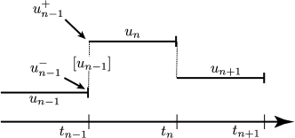
Figure 6: Visualization of the temporal jump of piecewise constant functions $u_{k}$ with $u_{n}=u_{k}\big{|}_{(t_{n-1},t_{n}]}$ at time point $t=t_{n}$.

For the formulation of the error estimator it is nevertheless essential to have the variational formulation (30) in mind, since the estimator relies on weighted residuals, i.e. on evaluations of (30) with test functions that come from a space of higher degree (e.g. $\phi_{h}=i_{k}^{(1)}z_{h}-z_{h}$, polynomials of degree 1). For higher order degree polynomials the box rule is not longer exact for evaluating the integrals and we must indeed use the variational formulation.

A.2 Galerkin orthogonality and partitioned solution

Both the real solution $u(t)$ to $u^{\prime}(t)=f(t,u(t))$ and the backward Euler approximation $u_{k}$ satisfy the variational formulation, $A(u,\phi)=0$ and $A(u_{k},\phi_{k})=0$, respectively. The difference is the choice of test functions $\phi$. While $u$ satisfies the variational problem for all test functions, $A(u_{k},\phi_{k})=0$ holds only for piecewise constant functions $\phi_{k}$. For these, Galerkin orthogonality is satisfied

$$A(u,\phi_{k})-A(u_{k},\phi_{k})=0.$$ (32)

Galerkin orthogonality plays an important role in the derivation of the dual weighted residual estimator, which, for simple linear problem takes the form

$$J(u)-J(u_{k})=A(u-u_{k},z),$$ (33)

where $z$ is the adjoint solution to $A(\psi,z)=J(\psi)$ for all test functions $\psi$. One problem, discussed in Remark 3 is the presence of the unknown solutions $u$ and $z$ that serve as weights of the estimator. By Galerkin orthogonality (32) we can add to (33) an interpolation of the adjoint solution $i_{k}z$

$$J(u)-J(u_{k})=A(u-u_{k},z-i_{k}z)=-A(u_{k},z-i_{k}z).$$ (34)

These new weights $z-i_{k}z$ are still not known (since they involve $z$). However, they can be efficiently approximated by reconstructing the interpolation error $z-i_{k}z$ in a space of higher order (linear functions instead of constants), again, see Remark 3 and we obtain the approximation

$$J(u)-J(u_{k})\approx-A(u_{k},i_{k}^{(1)}z_{k}-z_{k}).$$ (35)

This is the most simple primal form of the DWR method which is valid for linear models and linear functionals, compare Becker and Rannacher (2001). It only consists of the primal residual $A(u_{k},\cdot)$ weighted with the dual interpolation error $i_{k}^{(1)}z_{k}-z_{k}$. In Section 3 we must apply the more general form of the DWR method which also translates to nonlinear models like the sea ice momentum equation. Here, additional adjoint residuals, weighted with the primal interpolation errors $i_{k}^{(1)}u_{k}-u_{k}$ appear. In Figure 7 we illustrate this discrete reconstruction process $u_{k}\mapsto i_{k}^{(1)}u_{k}$.

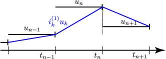
Figure 7: Reconstruction of the piecewise constant $u_{k}$ by piecewise linear polynomials for the evaluation of the weights.

Our discretization of the sea ice model is non-consisting, which means that the discrete problem is formulated via a modified variational formulation $A_{s}(u_{k},\phi_{k})=0$ with $A_{s}\neq A$, see Section 2.2 and in particular (11) where we define the form $B_{s}(U)(\Phi)$. One consequence of non-conformity is the violation of Galerkin orthogonality. For the partitioned solution approach, only the following disturbed relation holds

$$A(u,\phi_{k})-A_{s}(u_{k},\phi_{k})=-A(u_{k},\phi_{k}).$$

This non-consistency gives rise to the splitting terms of the error estimator denoted by $\beta$ in (20).

References

- (1)
- Afif et. al. (2003) \NAT@biblabelnumAfif et. al. 2003 Afif, M. ; Bergam, A. ; Mghazli, Z. ; Verfürth, R.: A posteriori estimators for the finite volume discretization of an elliptic problem. In: Numerical Algorithms 34 (2003), Nr. 2-4, pp. 127–136
- Becker et. al. (2019) \NAT@biblabelnumBecker et. al. 2019 Becker, R. ; Braack, M. ; Meidner, D. ; Richter, T. ; Vexler, B.: The finite element toolkit Gascoigne. 2019. – http://www.uni-kiel.de/gascoigne/
- Becker and Rannacher (2001) \NAT@biblabelnumBecker and Rannacher 2001 Becker, R. ; Rannacher, R.: An Optimal Control Approach to A Posteriori Error Estimation in Finite Element Methods. In: Iserles, A. (Hrsg.): Acta Numerica 2001 Bd. 37. Cambridge University Press, 2001, pp. 1–225
- Braack and Ern (2003) \NAT@biblabelnumBraack and Ern 2003 Braack, M. ; Ern, A.: A posteriori control of modeling errors and discretization errors. In: Multiscale Model. Simul. 1 (2003), Nr. 2, pp. 221–238
- Carpio et. al. (2013) \NAT@biblabelnumCarpio et. al. 2013 Carpio, J. ; Prieto, J.L. ; Bermejo, R.: Anisotropic “Goal-Oriented” Mesh Adaptivity for Elliptic Problems. In: SIAM Journal on Scientific Computing 35 (2013), Nr. 2, pp. A861–A885
- Chen and Gunzburger (2014) \NAT@biblabelnumChen and Gunzburger 2014 Chen, Q. ; Gunzburger, M.: Goal-oriented a posteriori error estimation for finite volume methods. In: J. of Comp. and Appl. Math. 265 (2014), pp. 69–82
- Collins et. al. (2014) \NAT@biblabelnumCollins et. al. 2014 Collins, J.B. ; Estep, D. ; Tavener, S.: A posteriori error estimation for the Lax–Wendroff finite difference scheme. In: J. Comp. Appl. Math. 263 (2014), pp. 299–311
- Coon (1980) \NAT@biblabelnumCoon 1980 Coon, M.D.: A review of AIDJEX modeling. In: Sea Ice Processes and Models: Symposium Proceedings, Univ. of Wash. Press, Seattle., 1980, pp. 12–27
- Danilov et. al. (2015) \NAT@biblabelnumDanilov et. al. 2015 Danilov, S. ; Wang, Q. ; Timmermann, R. ; Iakovlev, N. ; Sidorenko, D. ; Kimmritz, M. ; Jung, T. ; Schröter, J.: Finite-Element Sea Ice Model (FESIM), version 2. In: Geosci. Model Dev. 8 (2015), pp. 1747–1761
- Dansereau et. al. (2016) \NAT@biblabelnumDansereau et. al. 2016 Dansereau, V. ; Weiss, J. ; Saramito, P. ; Lattes, P.: A Maxwell elasto-brittle rheology for sea ice modelling. In: The Cryosphere 10 (2016), Nr. 3, pp. 1339–1359
- Griewank and Walther (2008) \NAT@biblabelnumGriewank and Walther 2008 Griewank, A. ; Walther, A.: Evaluating Derivatives: Principles and Techniques of Algorithmic Differentiation. 2. SIAM, 2008
- Heimbach et. al. (2005) \NAT@biblabelnumHeimbach et. al. 2005 Heimbach, P. ; Hill, C. ; Giering, R.: An efficient exact adjoint of the parallel MIT General Circulation Model, generated via automatic differentiation. In: Fut. Gen. Comp. Sys. 21 (2005), Nr. 8, pp. 1356–1371
- Hibler (1979) \NAT@biblabelnumHibler 1979 Hibler, W.D.: A dynamic thermodynamic sea ice model. In: J. Phys. Oceanogr 9 (1979), pp. 815–846
- Hunke and Dukowicz (1997) \NAT@biblabelnumHunke and Dukowicz 1997 Hunke, E.C. ; Dukowicz, J.K.: An elastic-viscous-plastic model for sea ice dynamics. In: J. Phys. Oceanogr. 27 (1997), pp. 1849–1867
- Hutter et. al. (2018) \NAT@biblabelnumHutter et. al. 2018 Hutter, N. ; Losch, M. ; Menemenlis, D.: Scaling properties of Arctic sea ice deformation in a high-resolution viscous-plastic sea ice model and in satellite observations. In: Journal of Geophysical Research 170 (2018), pp. 18–38
- Kimmritz et. al. (2016) \NAT@biblabelnumKimmritz et. al. 2016 Kimmritz, M. ; Danilov, S. ; Losch, M.: The adaptive EVP method for solving the sea ice momentum equation. In: Ocean Modelling 101 (2016), pp. 59–67
- Korn (2017) \NAT@biblabelnumKorn 2017 Korn, P.: Formulation of an unstructured grid model for global ocean dynamics. In: J. Comp. Phy. 339 (2017), pp. 525–552
- Kwok and Rothrock (2009) \NAT@biblabelnumKwok and Rothrock 2009 Kwok, R. ; Rothrock, D. A.: Decline in Arctic sea ice thickness from submarine and ICESat records: 1958–2008. In: Geophysical Research Letters 36 (2009), Nr. 15
- Lemieux et. al. (2014) \NAT@biblabelnumLemieux et. al. 2014 Lemieux, J.F. ; Knoll, D. ; Losch, M. ; Girard, C.: A second-order accurate in time IMplicit–EXplicit (IMEX) integration scheme for sea ice dynamics. In: J. Comp. Phys. 263 (2014), pp. 375–392
- Lemieux and Tremblay (2009) \NAT@biblabelnumLemieux and Tremblay 2009 Lemieux, J.F. ; Tremblay, B.: Numerical convergence of viscous-plastic sea ice models. In: J. Geophys. Res. 114 (2009), Nr. C5
- Lemieux et. al. (2010) \NAT@biblabelnumLemieux et. al. 2010 Lemieux, J.F. ; Tremblay, B. ; Sedláček, J. ; Tupper, P. ; Thomas, S. ; Huard, D. ; Auclair, J.P.: Improving the Numerical Convergence of Viscous-plastic Sea Ice Models with the Jacobian-free Newton-Krylov Method. In: J. Comp. Phys. 229 (2010), pp. 2840–2852
- Lipscomb et. al. (2007) \NAT@biblabelnumLipscomb et. al. 2007 Lipscomb, W. H. ; Hunke, E. C. ; Maslowski, W. ; Jakacki, J.: Ridging, strength and stability in high-resolution sea ice models. In: Journal of Geophysical Research 112 (2007)
- Marotzke et. al. (1999) \NAT@biblabelnumMarotzke et. al. 1999 Marotzke, J. ; Giering, R. ; Zhang, K.Q. ; Stammer, D. ; Hill, C. ; Lee, T.: Construction of the adjoint MIT ocean general circulation model and application to Atlantic heat transport sensitivity. In: J. of Geophys. Research Oceans 104 (1999), Nr. C12
- Mehlmann (2019) \NAT@biblabelnumMehlmann 2019 Mehlmann, C.: Efficient numerical methods to solve the viscous-plastic sea ice model at high spatial resolutions, Otto-von-Guericke Universität Magdeburg, Diss., 2019
- Mehlmann and Richter (2017a) \NAT@biblabelnumMehlmann and Richter 2017a Mehlmann, C. ; Richter, T.: A finite element multigrid-framework to solve the sea ice momentum equation. In: J. Comp. Phys. 348 (2017), pp. 847–861
- Mehlmann and Richter (2017b) \NAT@biblabelnumMehlmann and Richter 2017b Mehlmann, C. ; Richter, T.: A modified global Newton solver for viscous-plastic sea ice models. In: Ocean Modeling 116 (2017), pp. 96–107
- Meidner et. al. (2009) \NAT@biblabelnumMeidner et. al. 2009 Meidner, D. ; Rannacher, R. ; Vihharev, J.: Goal-oriented error control of the iterative solution of finite element equations. In: J. Num. Math. 17 (2009), Nr. 2
- Meidner and Richter (2014) \NAT@biblabelnumMeidner and Richter 2014 Meidner, D. ; Richter, T.: Goal-Oriented Error Estimation for the Fractional Step Theta Scheme. In: Comp. Meth. Appl. Math. 14 (2014), pp. 203–230
- Meidner and Richter (2015) \NAT@biblabelnumMeidner and Richter 2015 Meidner, D. ; Richter, T.: A Posteriori Error Estimation for the Fractional Step Theta discretization of the incompressible Navier-Stokes equations. In: Comp. Meth. Appl. Mech. Engrg. 288 (2015), pp. 45–59
- Quarteroni et. al. (2007) \NAT@biblabelnumQuarteroni et. al. 2007 Quarteroni, A. ; Sacco, R. ; Saleri, F.: Texts in Applied Mathematics. Bd. 37: Numerical Mathematics. Springer, 2007
- Rampal et. al. (2016) \NAT@biblabelnumRampal et. al. 2016 Rampal, P. ; Bouillon, S. ; Olason, E. ; Morlighem, M.: neXtSIM: a new Lagrangian sea ice model. In: The Cryosphere 10 (2016), pp. 1055–1073
- Richter (2017) \NAT@biblabelnumRichter 2017 Richter, T.: Fluid-structure Interactions. Springer International Publishing, 2017
- Richter and Wick (2015) \NAT@biblabelnumRichter and Wick 2015 Richter, T. ; Wick, T.: Variational Localizations of the Dual Weighted Residual Method. In: Journal of Computational and Applied Mathematics (2015), pp. 192–208
- Ringler et. al. (2013) \NAT@biblabelnumRingler et. al. 2013 Ringler, T. ; Petersen, M. ; Higdon, R. ; Jacobsen, D. ; Maltrud, M. ; Jones, P.: A multi-resolution approach to global ocean modelling. In: Ocean Modelling 69 (2013), pp. 211–232
- Schmich and Rannacher (2012) \NAT@biblabelnumSchmich and Rannacher 2012 Schmich, M. ; Rannacher, R.: Goal-oriented space–time adaptivity in the finite element Galerkin method for the computation of nonstationary incompressible flow. In: Int. J. Numer. Meth. Fluids 70 (2012), Nr. 1, pp. 1139–1166
- Schmich and Vexler (2008) \NAT@biblabelnumSchmich and Vexler 2008 Schmich, M. ; Vexler, B.: Adaptivity with dynamic meshes for space–time finite element discretizations of parabolic equations. In: SIAM Journal on Scientific Computing 30 (2008), Nr. 1, pp. 369–393
- Stroeve et. al. (2014) \NAT@biblabelnumStroeve et. al. 2014 Stroeve, J. ; Barrett, A .. ; Serreze, M. ; Schweiger, A.: Using records from submarine, aircraft and satellites to evaluate climate model. In: The Cryosphere 8 (2014), pp. 1839–1854
- Thomée (1997) \NAT@biblabelnumThomée 1997 Thomée, V.: Galerkin Finite Element Methods for Parabolic Problems. In: Springer Series in Computational Mathematics 25 (1997)
- Toyoda et. al. (2019) \NAT@biblabelnumToyoda et. al. 2019 Toyoda, T. ; Hirose, N. ; Urakawa, L.S. ; Tsujino, H. ; Nakano, H. ; Usui, N. ; Fujii, Y. ; Sakamoto, K. ; Yamanaka, G.: Effects of Inclusion of Adjoint Sea Ice Rheology on Backward Sensitivity Evolution Examined Using an Adjoint Ocean–Sea Ice Model. In: Mon. Wea. Rev. 147 (2019), Nr. 6, pp. 2145–2162
- Williams and Tremblay (2018) \NAT@biblabelnumWilliams and Tremblay 2018 Williams, J. ; Tremblay, B.: The dependence of energy dissipation on spatial resolution in a viscous-plastic sea-ice model. In: Ocean Modelling 130 (2018), pp. 40 – 47