Maximizing Products of Linear Forms, and
The Permanent of Positive Semidefinite Matrices

Abstract

We study the convex relaxation of a polynomial optimization problem, maximizing a product of linear forms over the complex sphere. We show that this convex program is also a relaxation of the permanent of Hermitian positive semidefinite (HPSD) matrices. By analyzing a constructive randomized rounding algorithm, we obtain an improved multiplicative approximation factor to the permanent of HPSD matrices, as well as computationally efficient certificates for this approximation. We also propose an analog of van der Waerden’s conjecture for HPSD matrices, where the polynomial optimization problem is interpreted as a relaxation of the permanent.

1 Introduction

We study the problem of maximizing a product of linear forms on the complex $(n-1)$-sphere of radius $\sqrt{n}$:

$$r(A)\equiv\max_{\left\lVert x\right\lVert^{2}=n}\prod_{i=1}^{n}\left|\left\langle x,v_{i}\right\rangle\right|^{2},$$ (1)

where $A=V^{\dagger}V$ and $v_{i}$ are the columns of $V$. We show that the natural convex relaxation of (1),

$$\max\,\prod_{i=1}^{n}v_{i}^{\dagger}Pv_{i}\,\mbox{ s.t. }\,\operatorname{Tr}(P)=n,\,P\succeq 0,$$ (2)

is also a relaxation of the permanent of $A$, which is defined by

$$\operatorname{per}(A)=\sum_{\sigma\in\mathbf{S}_{n}}\prod_{i=1}^{n}A_{i,\sigma(i)},$$ (3)

where the sum is over all $n!$ permutations of $n$ elements. Computing the permanent exactly is #P-hard [Val79], and approximation efforts have been focused on classes of matrices with computationally efficient certificates of permanent non-negativity. For matrices with non-negative entries, [JSV04] gave a randomized algorithm achieving a $(1+\epsilon)$-approximation. There has been recent interest in approximating the permanent of HPSD matrices due to their applications in quantum information [GS18]. The work by [AGGS17] gave the first polynomial-time algorithm for approximating the permanent of HPSD matrices with a simply exponential multiplicative approximation factor of $\frac{n!}{n^{n}}e^{-n\gamma}$, where $\gamma\approx 0.577$ is the Euler-Mascheroni constant. Their algorithm is based on the following convex program relaxation of the permanent.

Definition 1.1.

Given a HPSD matrix $A\in\mathbb{C}^{n\times n}$, we define $\operatorname{rel}(A)$ as the solution to the optimization problem:

$$\operatorname{rel}(A)\equiv\left\{\begin{array}[]{rl}\min&\prod_{i=1}^{n}D_{ii}\\ \text{s.t.}&A\preceq D,\quad D\text{ is diagonal}\end{array}\right.$$ (6)

In this paper, we show that $\operatorname{rel}(A)$ is equivalent to the convex relaxation (2). Our main result, Theorem 4.4, uses this connection between the polynomial optimization problem (1) and $\operatorname{per}(A)$ to provide a new analysis of the approximation of $\operatorname{per}(A)$ in terms of the rank of the optimal solution to (2). By bounding this rank, we prove an improved approximation factor for all finite $n$:

Corollary 1.2.

Given a HPSD matrix $A\in\mathbb{C}^{n\times n}$, $\operatorname{rel}(A)$ is an $\frac{n!}{n^{n}}e^{-nL_{r}}$-approximation to $\operatorname{per}(A)$:

$$\frac{n!}{n^{n}}e^{-nL_{r}}\operatorname{rel}(A)\leq\operatorname{per}(A)\leq\operatorname{rel}(A)$$

where $r=O(\sqrt{n})$, $L_{r}=H_{r-1}-\log(r)$, and $H_{r}=\sum_{k=1}^{r}\frac{1}{k}$ is the $r$-th harmonic number.

From the definition of the Euler-Mascheroni constant, $\lim_{n\rightarrow\infty}L_{r}=\gamma$. For any finite $n$, $L_{r}<\gamma$ and thus $\frac{n!}{n^{n}}e^{-nL_{r}}>\frac{n!}{n^{n}}e^{-n\gamma}$. More precisely, using Proposition A.1, we can show that this is a $e^{O(\sqrt{n})}$ multiplicative improvement. [AGGS17] also constructed a series of matrices $A_{k}$ such that $(\operatorname{rel}(A_{k})/\operatorname{per}(A_{k})))^{1/n}\rightarrow e^{1+\gamma}$ as $k\rightarrow\infty$. However since this result only rules out improvements on the order of $e^{O(n)}$, it does not contradict Corollary 1.2.

In Section 3 we analyze the convex relaxation of (1), describe a rounding procedure and prove its approximation factor. In particular we prove that

$$e^{-nL_{r}}\operatorname{rel}(A)\leq r(A)\leq\operatorname{rel}(A).$$

In Section 4 we prove Theorem 4.4. We first show that the convex relaxation of $r(A)$ is equivalent to $\operatorname{rel}(A)$. Then using the vector produced by the rounding procedure of the relaxation, we construct a rank-1 matrix whose permanent lower bounds $\operatorname{per}(A)$, thus showing that $\operatorname{rel}(A)$ also well-approximates $\operatorname{per}(A)$. Note that in [AGGS17] only the existence of this rank-1 matrix is shown, but in our analysis we provide an explicit construction of a rank-1 matrix whose permanent lower bounds $\operatorname{per}(A)$. This combined with the diagonal matrix in (6) whose permanent upper-bounds $\operatorname{per}(A)$ certifies the approximation. In Section 5 we explore reasons why the convex relaxation of (1) is equivalent to $\operatorname{rel}(A)$. We conjecture that (1) is itself a $\frac{n!}{n^{n}}$ approximation to $\operatorname{per}(A)$, explain why it is an analogue of van der Waerden’s conjecture, and show that it is implied by another long-standing permanent conjecture.

2 Preliminaries

For any $x\in\mathbb{C}$, let $x^{*}$ be its complex conjugate, and $\left|x\right|^{2}=xx^{*}$. For any matrix $A\in\mathbb{C}^{n\times m}$, let $A^{\dagger}=(A^{*})^{T}$ be its conjugate transpose. Given $a,b\in\mathbb{C}^{n}$, let $\left\langle a,b\right\rangle=a^{\dagger}b$ be the inner product on the Hilbert space $\mathbb{C}^{n}$, and $\left\lVert a\right\lVert^{2}=\left\langle a,a\right\rangle$. Let $S_{\mathbb{C}}(n)=\{x\in\mathbb{C}^{n}\mid\left\lVert x\right\lVert^{2}=n\}$ be the complex sphere in $n$ dimensions of radius $\sqrt{n}$. A matrix $A$ is Hermitian if $A=A^{\dagger}$, and is Hermitian positive semidefinite (HPSD) if in addition $x^{\dagger}Ax\geq 0$ for all $x\in\mathbb{C}^{n}$. We can also denote this as $A\succeq 0$. The $\succeq$ operator induces a partial order called the Löwner order, where $A\succeq B$ if $A-B\succeq 0$. If $A\succeq 0$, it can be factorized as $A=L^{\dagger}L$, where $L\in\mathbb{C}^{n\times n}$ (for example by the Cholesky decomposition).

2.1 Circularly-Symmetric Gaussian Random Variables

In this paper we will use a few results involving vectors of circularly-symmetric valued Gaussian variables.

Definition 2.1 (Circularly-symmetric Gaussian random vector).

The complex-valued Gaussian random variable $Z=Z_{r}+iZ_{c}$ is circularly-symmetric if $Z_{r}$ and $Z_{c}$ are i.i.d. drawn from $\mathcal{N}(0,\frac{1}{2})$. The random vector $\mathbf{Z}=[Z_{1},\ldots,Z_{n}]^{T}$ is drawn from the distribution $\mathcal{C}\mathcal{N}(0,\Sigma)$ if $Z_{i}$ are i.i.d. circularly-symmetric Gaussians and $\mathop{{}\mathbb{E}}[\mathbf{Z}\mathbf{Z}^{\dagger}]=\Sigma$.

The name circularly-symmetric comes from the fact that $\mathbf{Z}$ is invariant under rotations in the complex plane, meaning that $e^{i\theta}\mathbf{Z}$ has the same distribution as $\mathbf{Z}$ for all real $\theta$. All complex multivariate Gaussians in this paper are circularly symmetric. Similar to real multivariate Gaussians, a linear transform on the random vector induces a congruence transform on the covariance matrix.

Proposition 2.2 (Linear transformations of complex multivariate Gaussians).

Given $\mathbf{Z}\sim\mathcal{C}\mathcal{N}(0,\Sigma)$ and any complex matrix $A$, $A\mathbf{Z}$ is also circularly symmetric and has the distribution $\mathcal{C}\mathcal{N}(0,A\Sigma A^{\dagger})$.

The proof of this proposition and more about complex multivariate Gaussians can be found in [Gal]. In particular, this tells us that $\mathbf{Z}\sim\mathcal{C}\mathcal{N}(0,I)$ is invariant under unitary transformations.

In the analysis of our rounding procedure, we use some results about the gamma distribution.

Fact 2.3 (Expectation of log of gamma random variable).

Let $X\sim\operatorname{Gamma}(\alpha,\beta)$ be drawn from the gamma distribution, with density $p(x;\alpha,\beta)=\Gamma(\alpha)^{-1}\beta^{\alpha}x^{\alpha-1}e^{-\beta x}$. Then

$$\mathop{{}\mathbb{E}}[\log X]=\psi(\alpha)-\log(\beta),$$

where $\psi(x)=\frac{d}{dx}\log\Gamma(x)$ is the digamma function.

This follows from the fact that the gamma distribution is an exponential family, and $\log x$ is a sufficient statistic (see section 2.2 of [Kee10] for more details). Next we prove a useful identity.

Fact 2.4.

Let $[z_{1},\ldots,z_{r}]^{T}\sim\mathcal{C}\mathcal{N}(0,I_{r})$, $H_{n}=\sum_{k=1}^{n}\frac{1}{k}$ be the $n$-th harmonic number and $\gamma=\lim_{n\rightarrow\infty}(H_{n}-\log n)$ be the Euler-Mascheroni constant. Then

$$\mathop{{}\mathbb{E}}\log\left(\frac{1}{r}\sum_{i=1}^{r}\left|z_{i}\right|^{2}\right)=H_{r-1}-\gamma-\log(r)=L_{r}-\gamma.$$

Proof.

$\sum_{i=1}^{r}2\left|z_{i}\right|^{2}$ is distributed as a chi-squared distribution with $2r$ degrees of freedom, which is equivalent to $\operatorname{Gamma}\left(r,\frac{1}{2}\right)$. Using Fact 2.3, $\mathop{{}\mathbb{E}}\log\left(\sum_{i=1}^{r}\left|z_{i}\right|^{2}\right)=\psi(r)$. Since $\psi(1)=-\gamma$ by Gauss’s digamma theorem, the recurrence relation of the gamma function shows that for all positive integers $r$, $\psi(r)=H_{r-1}-\gamma$. ∎

Integrating a homogeneous polynomial over the complex sphere is equivalent to taking its expectation with respect to $x\sim\mathcal{C}\mathcal{N}(0,I)$, up to a correction factor. This factor can be found by computing moments of a chi-squared distribution.

Fact 2.5.

Let $p(x)$ be a degree $d$ homogeneous polynomial in $n$ variables, $\mu_{n}(x)$ be the measure associated with the random variable $x\sim\mathcal{C}\mathcal{N}(0,I_{n})$. Then

$$\int\displaylimits_{\mathbb{C}^{n}}\left|p(x)\right|^{2}\,d\mu_{n}(x)=\frac{(n+d-1)!}{n^{n}(n-1)!}\int\displaylimits_{S_{\mathbb{C}}(n)}\left|p(x)\right|^{2}\,dx.$$

2.2 Permanent of HPSD Matrices

One remarkable property of the permanent of HPSD matrices is that it respects the Löwner order. See section 2.3 of [AGGS17] for a proof.

Proposition 2.6.

If $A\succeq B\succeq 0$, then $\operatorname{per}(A)\geq\operatorname{per}(B)\geq 0$.

We can efficiently compute the permanent of rank-1 matrices. The following proposition immediately follows from the definition of the permanent in (3).

Proposition 2.7.

For any $v\in\mathbb{C}^{n}$, $\operatorname{per}(vv^{\dagger})=n!\prod_{i=1}^{n}\left|v_{i}\right|^{2}$.

The permanent of HPSD matrices also has an integral representation using complex multivariate Gaussians. See section 4 of [Bar07] for more details and a proof.

Proposition 2.8.

Let $\mu_{n}(x)$ be the measure associated with the random variable $x\sim\mathcal{C}\mathcal{N}(0,I_{n})$, and $S_{\mathbb{C}}(n)$ be the complex $(n-1)$-sphere with radius $\sqrt{n}$. For any HPSD $A=V^{\dagger}V$, where $v_{i}$ are the columns of $V$,

$$\operatorname{per}(A)=\int\displaylimits_{\mathbb{C}^{n}}\prod_{i=1}^{n}\left|\left\langle v_{i},x\right\rangle\right|^{2}\,d\mu_{n}(x)=\frac{(2n-1)!}{n^{n}(n-1)!}\int\displaylimits_{S_{\mathbb{C}}(n)}\prod_{i=1}^{n}\left|\left\langle v_{i},x\right\rangle\right|^{2}\,dx.$$

3 Convex Relaxation and Rounding

In this section we analyze the convex relaxation (2) and a natural rounding algorithm for maximizing a product of linear forms over the complex sphere.

Remark 3.1.

Both $r(A)$ and $\operatorname{rel}(A)$ are independent of the factorization of $A=V^{\dagger}V$. This is because any two different factorizations of $A=V_{1}^{\dagger}V_{1}=V_{2}^{\dagger}V_{2}$ are related by a unitary transform $V_{1}=UV_{2}$ for some unitary matrix $U$ . This induces a change of variables $x\mapsto U^{\dagger}x$ in (1) but does not change the value of $r(A)$.

Lemma 3.2.

Any $A\succeq 0$ can be factorized as $A=V^{\dagger}V$, where $v_{i}$ are the columns of $V$. Consider the following pair of convex programs:

$$\mu^{*}(A)\,\equiv\, \min\,\,\lambda^{n}\,\mbox{ s.t. }\,\left\{\begin{array}[]{rl}V\operatorname{Diag}(\alpha)V^{\dagger}&\preceq\lambda I_{n}\\ \prod_{i=1}^{n}\alpha_{i}&\geq 1\\ \alpha_{i}&>0\end{array}\right.$$ (10)

$$\nu^{*}(A)\,\equiv\, \max\,\,\prod_{i=1}^{n}v_{i}^{\dagger}Pv_{i}\,\mbox{ s.t. }\,\left\{\begin{array}[]{rl}\operatorname{Tr}(P)&=n\\ P^{\dagger}&=P\\ P&\succeq 0\end{array}\right.$$ (14)

Then $r(A)\leq\nu^{*}(A)=\mu^{*}(A)$, thus the convex programs are relaxations of $r(A)$ (see equation (1)).

Proof.

If we add a rank-1 constraint to (14), we get (1), showing that $r(A)\leq\nu^{*}(A)$. Suppose we have feasible solutions $\lambda$, $\alpha_{i}$ and $P$ to (10) and (14) respectively. Then

$$\prod_{i=1}^{n}v_{i}^{\dagger}Pv_{i}=\prod_{i=1}^{n}\alpha_{i}v_{i}^{\dagger}Pv_{i}\leq\left(\frac{1}{n}\sum_{i=1}^{n}\alpha_{i}v_{i}^{\dagger}Pv_{i}\right)^{n}\leq\left(\frac{\operatorname{Tr}(P)\lambda}{n}\right)^{n}=\lambda^{n},$$

showing weak duality, i.e. $\nu^{*}(A)\leq\mu^{*}(A)$. Since (14) comes from taking the dual of (10) and has a strictly feasible solution, strong duality holds, i.e. $\nu^{*}(A)=\mu^{*}(A)$. If $P=xx^{\dagger}$ is rank-1, then $v_{i}^{\dagger}Pv_{i}=\left|\left\langle x,v_{i}\right\rangle\right|^{2}$, thus in (14) the variable $P$ can be interpreted as the convex relaxation of the rank-1 constraint in (1). ∎

Although (10) and (14) have non-linear objective functions and are not semidefinite programs in standard form, the geometric mean constraint/objective in them can be converted to second-order conic constraints after a change of variables [LVBL98]. They can also be solved efficiently with convex programming techniques such as interior point methods (see [VBW98]). Our main result (Theorem 4.4) is proven with the following analysis of a randomized rounding procedure to the convex relaxation of the product of linear forms. This produces a vector that gives an $e^{-nL_{r}}$-approximation to (1).

Theorem 3.3.

Given a matrix $A\succeq 0$, let $\nu^{*}(A)$ be the optimum of (14), with optimum achieved by $P^{*}=UU^{\dagger}$. Suppose $P^{*}$ has rank $r$, therefore $U\in\mathbb{C}^{n\times r}$. If we produce a vector $y\in S_{\mathbb{C}}(n)$ using the following procedure:

1. Sample $z\in\mathbb{C}^{r}$ uniformly at random from the complex multivariate Gaussian $\mathcal{C}\mathcal{N}(0,I_{r})$

2. Return the normalized vector $y=\sqrt{n}Uz/\left\lVert Uz\right\lVert$

Recalling that $L_{r}=H_{r-1}-\log r$, we have the following lower bound on the expected value of the objective:

$$\mathop{{}\mathbb{E}}_{z}\left[\prod_{i=1}^{n}\left|\left\langle v_{i},y\right\rangle\right|^{2}\right]\geq e^{-nL_{r}}\nu^{*}(A)$$

Proof.

We use Jensen’s inequality to bound the expectation:

$$\mathop{{}\mathbb{E}}_{z}\left[\prod_{i=1}^{n}\frac{n\left|\left\langle v_{i},Uz\right\rangle\right|^{2}}{\left\lVert Uz\right\lVert^{2}}\right] =\mathop{{}\mathbb{E}}_{z}\left[\exp\left(\sum_{i=1}^{n}(\log\left|\left\langle v_{i},Uz\right\rangle\right|^{2}-\log z^{\dagger}U^{\dagger}Uz+\log n)\right)\right]$$

$$\geq\exp\left(\sum_{i=1}^{n}(\mathop{{}\mathbb{E}}_{z}\log\left|\left\langle v_{i},Uz\right\rangle\right|^{2}-\mathop{{}\mathbb{E}}_{z}\log z^{\dagger}U^{\dagger}Uz+\log n)\right)$$

We can exactly compute the first expectation:

$$\mathop{{}\mathbb{E}}_{z}\log\left|\left\langle v_{i},Uz\right\rangle\right|^{2} =\log v_{i}^{\dagger}UU^{\dagger}v_{i}+\mathop{{}\mathbb{E}}_{z}\log\left|\left\langle U^{\dagger}v_{i}/\left\lVert U^{\dagger}v_{i}\right\lVert,z\right\rangle\right|^{2}$$

$$=\log v_{i}^{\dagger}UU^{\dagger}v_{i}+\mathop{{}\mathbb{E}}_{z}\log\left|z_{1}\right|^{2}$$

$$=\log v_{i}^{\dagger}P^{*}v_{i}-\gamma$$

Where the first equality follows from normalizing $U^{\dagger}v_{i}$, the second equality follows from the rotational symmetry of the complex multivariate Gaussian since $U^{\dagger}v_{i}/\left\lVert U^{\dagger}v_{i}\right\lVert$ is a unit vector, and the third equality follows from Fact 2.4 for $r=1$. Let $\lambda_{1},\ldots,\lambda_{r}$ be the eigenvalues of $U^{\dagger}U$. Then

$$\mathop{{}\mathbb{E}}_{z}\log z^{\dagger}U^{\dagger}Uz=\mathop{{}\mathbb{E}}_{z}\log\left(\sum_{i=1}^{r}\lambda_{i}\left|z_{i}\right|^{2}\right)\leq\mathop{{}\mathbb{E}}_{z}\log\left(\frac{n}{r}\sum_{i=1}^{r}\left|z_{i}\right|^{2}\right)=H_{r-1}-\gamma+\log\left(\frac{n}{r}\right),$$

where the first equality follows from the invariance of the complex multivariate Gaussian under unitary transformations (see Proposition 2.2), and the second equality follows from Fact 2.4. Next we prove the inequality. Since $\operatorname{Tr}(U^{\dagger}U)=\operatorname{Tr}(P^{*})=n$, $\lambda=(\lambda_{1},\ldots,\lambda_{r})$ lies on the scaled $r$-simplex. The function $\lambda\mapsto\mathop{{}\mathbb{E}}_{z}\log\left(\sum_{i=1}^{r}\lambda_{i}\left|z_{i}\right|^{2}\right)$ is concave on the scaled $r$-simplex and is symmetric with respect to all permutations of the coordinates of $\lambda$, therefore it is maximized when all $\lambda_{i}=\frac{n}{r}$. Finally we put the above together, along with the fact that $\prod_{i=1}^{n}v_{i}^{\dagger}P^{*}v_{i}=\nu^{*}(A)$, to prove the theorem. ∎

4 Approximating the Permanent

We present a new analysis of the relaxation of the permanent of HPSD matrices in [AGGS17]. First we show that $\operatorname{rel}(A)$ is a relaxation of $\operatorname{per}(A)$.

Lemma 4.1.

Given any $A\succeq 0$,

$$\operatorname{per}(A)\leq\operatorname{rel}(A).$$

Proof.

Using the monotonicity of the permanent with respect to the Löwner order (Proposition 2.6), $A\preceq D$ implies that $\operatorname{per}(A)\leq\operatorname{per}(D)$. Since $D$ is diagonal, $\operatorname{per}(D)=\prod_{i}D_{ii}$, showing that the permanent is always bounded by $\operatorname{rel}(A)$. ∎

Next we show that $\operatorname{rel}(A)$ is equivalent to the convex relaxation of (1).

Lemma 4.2.

Recall that $\mu^{*}(A)=\nu^{*}(A)$ is the optimal value of the convex relaxation in Lemma 3.2. Then

$$\operatorname{rel}(A)=\mu^{*}(A)=\nu^{*}(A).$$

Proof.

By a scaling argument, the optimum of (10) is achieved when $\prod_{i}\alpha_{i}=1$. Taking Schur complements, $V\operatorname{Diag}(\alpha)V^{\dagger}\preceq\lambda I_{n}$ is equivalent to $\lambda\operatorname{Diag}(\alpha)^{-1}\succeq V^{\dagger}V=A$. Thus by making the substitution $D_{ii}=\lambda/\alpha_{i}$ and noting that $\prod_{i}D_{ii}=\lambda^{n}$, we show that $\operatorname{rel}(A)=\mu^{*}(A)$. ∎

The following lemma shows that given any vector $y\in S_{\mathbb{C}}(n)$ returned by the rounding algorithm, we can construct a lower bound on $\operatorname{per}(A)$.

Lemma 4.3.

Given HPSD $A=V^{\dagger}V\in\mathbb{C}^{n\times n}$, where $v_{i}$ are columns of $V$, and a vector $y\in S_{\mathbb{C}}(n)$,

$$\frac{n!}{n^{n}}\prod_{i=1}^{n}\left|\left\langle v_{i},y\right\rangle\right|^{2}\leq\operatorname{per}(A).$$

Proof.

Since $\left\lVert y\right\lVert^{2}=n$, $yy^{\dagger}\preceq nI$ and $V^{\dagger}yy^{\dagger}V\preceq nV^{\dagger}V$. Thus $n^{-n}\operatorname{per}(V^{\dagger}yy^{\dagger}V)\leq\operatorname{per}(V^{\dagger}V)=\operatorname{per}(A)$. Since $V^{\dagger}yy^{\dagger}V$ is a rank-1 matrix, its permanent is $n!\prod_{i}\left|\left\langle v_{i},y\right\rangle\right|^{2}$ by Proposition 2.7. ∎

Now we can state our result about approximating the permanent of a HPSD matrix.

Theorem 4.4.

Given a HPSD matrix $A\in\mathbb{C}^{n\times n}$, $\operatorname{rel}(A)$ is a relaxation of $\operatorname{per}(A)$ computable in polynomial-time by convex programs (10) or (14). Let $r$ be the rank of $P^{*}$, the solution to (14). Then $\operatorname{rel}(A)$ is an $\frac{n!}{n^{n}}e^{-nL_{r}}$-approximation to $\operatorname{per}(A)$:

$$\frac{n!}{n^{n}}e^{-nL_{r}}\operatorname{rel}(A)\leq\operatorname{per}(A)\leq\operatorname{rel}(A)$$ (15)

Next we state a result that we will use to bound the rank of $P^{*}$.

Lemma 4.5 (Theorem 2.2 in [AHZ08]).

Suppose there is a non-zero solution $X$ to the system of equations $\{X\succeq 0,\operatorname{Tr}(A_{i}X)=b_{i},\,i=1,\ldots,d\}$, where $A_{i}$ is Hermitian and $b_{i}\in\mathbb{C}$. If $d<(r+1)^{2}$, then one can find in polynomial time another solution $X^{\prime}$ where $\operatorname{rank}(X^{\prime})=r$.

We can now prove Corollary 1.2.

Proof of Corollary 1.2.

Given a solution $P$ to (14), any HPSD matrix $P^{\prime}$ that satisfy the $n+1$ equalities $\operatorname{Tr}(v_{i}v_{i}^{\dagger}P^{\prime})=v_{i}^{\dagger}Pv_{i}$ and $\operatorname{Tr}(P^{\prime})=n$ will have the same objective value as that of $P$. Applying Lemma 4.5, we can find in polynomial time an optimal solution $P^{*}$ with $\operatorname{rank}(P^{*})\leq O(\sqrt{n})$. We then apply Theorem 4.4. ∎

Finally we prove Theorem 4.4.

Proof of Theorem 4.4.

We use the vector $y$ produced in the rounding procedure in Theorem 3.3 to construct a rank-1 matrix $V^{\dagger}yy^{\dagger}V$. We then compare the permanent of this matrix to $\operatorname{per}(A)$ and $\operatorname{rel}(A)$:

$$\frac{n!}{n^{n}}e^{-nL_{r}}\operatorname{rel}(A)\stackrel{{\scriptstyle 1}}{{=}}\frac{n!}{n^{n}}\,e^{-nL_{r}}\nu^{*}(A)\stackrel{{\scriptstyle 2}}{{\leq}}\frac{n!}{n^{n}}\,\mathop{{}\mathbb{E}}\left[\prod_{i=1}^{n}\left|\left\langle v_{i},y\right\rangle\right|^{2}\right]\stackrel{{\scriptstyle 3}}{{\leq}}\operatorname{per}(A)\stackrel{{\scriptstyle 4}}{{\leq}}\operatorname{rel}(A)$$

1. Apply Lemma 4.2.

2. Apply Theorem 3.3.

3. Lemma 4.3 shows that for any vector $y\in S_{\mathbb{C}}(n)$, $\operatorname{per}(A)\geq\frac{n!}{n^{n}}\prod_{i=1}^{n}\left|\left\langle v_{i},y\right\rangle\right|^{2}$. This is also true when taking an expectation of any distribution supported on $S_{\mathbb{C}}(n)$.

4. Apply Lemma 4.1.

∎

4.1 Low Rank Instances

There are structured classes of HPSD matrices where we can prove a priori that the rank of $P^{*}$ is low and thus a better approximation ratio can be obtained. For example, it is easy to show that $\operatorname{rank}(P^{*})\leq\operatorname{rank}(A)$. Often such instances also have additional symmetry, such as the class of circulant matrices.

Corollary 4.6.

A square matrix is circulant if each row is cyclically shifted one position to the right compared to the previous row. If $A\in\mathbb{C}^{n\times n}$ is HPSD and circulant, then there is a solution $P^{*}$ to (14) where $\operatorname{rank}(P^{*})=1$ and we have the bound

$$\frac{n!}{n^{n}}\operatorname{rel}(A)\leq\operatorname{per}(A)\leq\operatorname{rel}(A).$$

Proof.

Since $A=V^{\dagger}V$ is circulant it is invariant under the map $A_{i,j}\mapsto A_{(i+1\mod n),(j+1\mod n)}$. Suppose we have an optimal solution $D^{*}$ to $\operatorname{rel}(A)$ in (6), where $D^{*}$ is a diagonal matrix satisfying $A\preceq D^{*}$. We then average over all cyclic shifts of $D^{*}$ to show that $D=\lambda I$ is also optimal, which corresponds to $\alpha_{i}=1$ in (10), with an optimal solution $P$ of (14) satisfying the complementary slackness condition of $\operatorname{Tr}(PVV^{\dagger})=n\lambda$. This shows that $P=vv^{\dagger}$ is also a solution, where $v$ is a suitable multiple of the top eigenvector of $VV^{\dagger}$. ∎

We also observed experimentally that $\operatorname{rank}(P^{*})$ is small for random $A$. Figure 1 plots this rank as a function of $n$, for instances of $A$ drawn from the Gaussian orthogonal ensemble. The results suggest that $\operatorname{rank}(P^{*})$ for these random instances grows slower than $O(\sqrt{n})$.

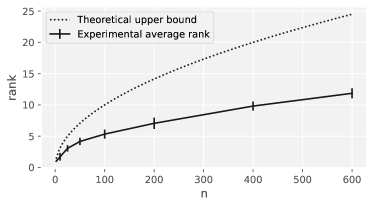
Figure 1: Plot of average of $\operatorname{rank}(P^{*})$ (along with error bars indicating standard deviation) of 50 random instances as a function of $n$. $A=V^{\dagger}V$ is constructed by sampling each entry of $V\in\mathbb{R}^{n\times n}$ from a standard Gaussian. The theoretical upper bound for $\operatorname{rank}(P^{*})$ in Lemma 4.5 is also shown for comparison.

5 A Conjecture

Our analysis of $\operatorname{rel}(A)$ was inspired by the optimization problem (1), maximizing a product of linear forms over the complex sphere. We conjecture that the exact solution to this optimization problem is a tighter relaxation of the permanent.

Conjecture 5.1.

Given $A=V^{\dagger}V$, where $v_{i}$ are the columns of $V$, recall that $r(A)$ is the maximum of a product of linear forms as defined in (1). Then

$$\frac{n!}{n^{n}}r(A)\leq\operatorname{per}(A)\leq r(A).$$ (16)

If the matrix $A$ is scaled so that $r(A)=1$, then (16) is exactly the same bounds given by the van der Waerden’s conjecture for doubly stochastic matrices (proved by [Fal81], [Ego81] [Gur08]). The lower bound follows from Lemma 4.3, but the upper bound cannot be proven by naively applying Proposition 2.8 and bounding the integral over the complex sphere by its maximum. However, we can show that the upper bound is implied by another conjecture on permanents:

Conjecture 5.2 (Pate’s conjecture [Pat84]).

Given any $n\times n$ HPSD matrix $A$, let $A\otimes J_{k}$ be the Kronecker product of $A$ with the $k\times k$ all-ones matrix. Then

$$\operatorname{per}(A\otimes J_{k})\geq\operatorname{per}(A)^{k}(k!)^{n}.$$ (17)

This conjecture has been proved in the case where $n=2$, see [Zha16] for a survey of subsequent progress on this conjecture. Using the integral representation of the permanent (Proposition 2.8), we can write (17) as:

$$\mathop{{}\mathbb{E}}_{x\sim\mathcal{C}\mathcal{N}(0,I_{n})}\left[\prod_{i=1}^{n}\left|\left\langle v_{i},x\right\rangle\right|^{2k}\right]^{1/k}\geq\operatorname{per}(A)\mathop{{}\mathbb{E}}_{x\sim\mathcal{C}\mathcal{N}(0,I_{n})}\left[\prod_{i=1}^{n}\left|x_{i}\right|^{2k}\right]^{1/k}$$

Since both expectations are taken over homogeneous polynomials of degree $d$, we can apply Fact 2.5, take $k\rightarrow\infty$ and get:

$$\max_{\left\lVert x\right\lVert^{2}=n}\prod_{i=1}^{n}\left|\left\langle v_{i},x\right\rangle\right|^{2}\geq\operatorname{per}(A)\max_{\left\lVert x\right\lVert^{2}=n}\prod_{i=1}^{n}\left|x_{i}\right|^{2}=\operatorname{per}(A).$$

6 Discussion and Conclusion

There are a few interesting directions that stem from this work. For random $A$ (i.e. drawn from the Gaussian orthogonal ensemble), numerical experiments in Section 4.1 suggest that $\operatorname{rank}(P^{*})$ is very small compared to $\sqrt{n}$. It would be interesting to provide concrete bounds on the rank of random instances. One might also ask if we can construct sequences of matrices $A_{k}$ of increasing size but with fixed rank $r$, where $(\operatorname{rel}(A_{k})/\operatorname{per}(A_{k}))^{1/n}\rightarrow e^{1+L_{r}}$. This is related to the question called the linear polarization constant of Hilbert spaces, see [PR04] for such a construction and its analysis.

The main result of this paper uses the connection between the permanent and the optimization of a product of linear forms over the sphere (1). Although it is natural to conjecture the hardness of computing $r(A)$, we do not know of any formal results establishing this. We also proposed Conjecture 5.1 which would explain why this optimization problem is intimately related to the permanent. Better understanding of this problem may lead to further insights about the permanent of HPSD matrices.

Appendix A Asymptotics of the Approximation Factor

Proposition A.1.

For all positive integers $r$,

$$\frac{1}{2r}<\gamma-L_{r}<\frac{r+2}{2r(r+1)}.$$ (18)

Proof.

It is easy to see that (18) follows from

$$\frac{1}{2(r+1)}<H_{n}-\log(r)-\gamma<\frac{1}{2r}.$$

From Figure 2, we can see that $H_{n}-\log(r)-\gamma=\sum_{k=r}^{\infty}\Delta_{k}$. The upper bound is given by computing the sum of the areas of the larger triangles:

$$\sum_{k=r}^{\infty}\Delta_{k}<\sum_{k=r}^{\infty}\frac{1}{2}\left(\frac{1}{k}-\frac{1}{k+1}\right)=\sum_{k=r}^{\infty}\frac{1}{2k(k+1)}=\frac{1}{2r}$$

The lower bound is given by computing the sum of the areas of the smaller triangles:

$$\sum_{k=r}^{\infty}\Delta_{k}>\sum_{k=r}^{\infty}\frac{1}{2}\frac{1}{(k+1)^{2}}>\sum_{k=r}^{\infty}\frac{1}{2(k+1)(k+2)}=\frac{1}{2(r+1)}$$

Figure 2: Illustration of the asymptotics of $L_{r}$. $\Delta_{r}$ is the area between the curve $y=\frac{1}{x}$ and the rectangle of height $\frac{1}{r+1}$. The lower dotted lines are tangent to the curve at $r+1$ and $r+2$ respectively.

∎

References

- [AGGS17] Nima Anari, Leonid Gurvits, Shayan Oveis Gharan, and Amin Saberi, Simply Exponential Approximation of the Permanent of Positive Semidefinite Matrices, 2017 IEEE 58th Annual Symposium on Foundations of Computer Science (FOCS), October 2017, pp. 914–925.
- [AHZ08] Wenbao Ai, Yongwei Huang, and Shuzhong Zhang, On the Low Rank Solutions for Linear Matrix Inequalities, Mathematics of Operations Research 33 (2008), no. 4, 965–975.
- [Bar07] Alexander Barvinok, Integration and Optimization of Multivariate Polynomials by Restriction Onto a Random Subspace, Found. Comput. Math. 7 (2007), no. 2, 229–244.
- [Ego81] G.P Egorychev, The solution of van der Waerden’s problem for permanents, Advances in Mathematics 42 (1981), no. 3, 299–305 (en).
- [Fal81] D. I. Falikman, Proof of the van der Waerden conjecture regarding the permanent of a doubly stochastic matrix, Mathematical notes of the Academy of Sciences of the USSR 29 (1981), no. 6, 475–479 (en).
- [Gal] Robert G Gallager, Circularly-Symmetric Gaussian random vectors, http://www.rle.mit.edu/rgallager/documents/CircSymGauss.pdf.
- [GS18] Daniel Grier and Luke Schaeffer, New hardness results for the permanent using linear optics, Proceedings of the 33rd Computational Complexity Conference (San Diego, California), CCC ’18, Schloss Dagstuhl–Leibniz-Zentrum fuer Informatik, June 2018, pp. 1–29.
- [Gur08] Leonid Gurvits, Van der Waerden/Schrijver-Valiant like Conjectures and Stable (aka Hyperbolic) Homogeneous Polynomials : One Theorem for all, The Electronic Journal of Combinatorics 15 (2008).
- [JSV04] Mark Jerrum, Alistair Sinclair, and Eric Vigoda, A Polynomial-time Approximation Algorithm for the Permanent of a Matrix with Nonnegative Entries, J. ACM 51 (2004), no. 4, 671–697.
- [Kee10] Robert W. Keener, Theoretical statistics: Topics for a core course, Springer Texts in Statistics, Springer, New York, 2010 (en).
- [LVBL98] Miguel Sousa Lobo, Lieven Vandenberghe, Stephen Boyd, and Hervé Lebret, Applications of second-order cone programming, Linear Algebra and its Applications 284 (1998), no. 1-3, 193–228 (en).
- [Pat84] Thomas H. Pate, An inequality involving permanents of certain direct products, Linear Algebra and its Applications 57 (1984), 147–155 (en).
- [PR04] Alexandros Pappas and Szilárd Gy. Révész, Linear polarization constants of Hilbert spaces, Journal of Mathematical Analysis and Applications 300 (2004), no. 1, 129–146 (en).
- [Val79] L.G. Valiant, The complexity of computing the permanent, Theoretical Computer Science 8 (1979), no. 2, 189–201 (en).
- [VBW98] Lieven Vandenberghe, Stephen Boyd, and Shao-Po Wu, Determinant Maximization with Linear Matrix Inequality Constraints, SIAM Journal on Matrix Analysis and Applications 19 (1998), no. 2, 499–533 (en).
- [Zha16] Fuzhen Zhang, An update on a few permanent conjectures, Special Matrices 4 (2016), no. 1 (en).