Flavor-changing decay $h\to\tau\mu$ at super hadron colliders

Abstract

We study the flavor-changing decay $h\to\tau\mu$ with $\tau=\tau^{-}+\tau^{+}$ and $\mu=\mu^{-}+\mu^{+}$ of a Higgs boson at future hadron colliders, namely: a) High Luminosity Large Hadron Collider, b) High Energy Large Hadron Collider and c) Future hadron-hadron Circular Collider. The theoretical framework adopted is the Two-Higgs-Doublet Model type III. The free model parameters involved in the calculation are constrained through Higgs boson data, Lepton Flavor Violating processes and the muon anomalous magnetic dipole moment; later they are used to analyze the branching ratio of the decay $h\to\tau\mu$ and to evaluate the $gg\to h$ production cross section. We find that at the Large Hadron Collider is not possible to claim for evidence of the decay $h\to\tau\mu$ achieving a signal significance about of $1.46\sigma$ by considering its final integrated luminosity, 300 fb^-1. More promising results arise at the High Luminosity Large Hadron Collider in which a prediction of 4.6$\sigma$ when an integrated luminosity of 3 ab^-1 and $\tan\beta=8$ are achieved. Meanwhile, at the High Energy Large Hadron Collider (Future hadron-hadron Circular Collider) a potential discovery could be claimed with a signal significance around $5.04\sigma$ ($5.43\sigma$) for an integrated luminosity of 3 ab^-1 and $\tan\beta=8$ (5 ab^-1 and $\tan\beta=4$).

1 Introduction

A lepton flavor violation (LFV) is a transition between $e$, $\mu$, $\tau$ sectors that does not conserve lepton family number. Within the Standard Model (SM) with massless neutrinos, individual lepton number is conserved. Even with the addition of non-zero neutrino masses, processes that violate charged lepton number are suppressed by powers of $m^{2}_{\nu}/m^{2}_{W}$ raidal and they should be extremely sensitive to physics beyond the SM (BSM). Neutrino oscillations are a quantum mechanical consequence of the existence of nonzero neutrino masses and mixings. The experiments with solar, atmospheric, reactor and accelerator neutrinos ahmad ; eguchi ; fukuda ; ahn have provided evidences for the existence of this phenomenon pontecorvo ; maki giving a clear signal of LFV. On the other hand, the observation of charged lepton flavor-violating (CLFV) processes would be a non-trivial signal of physics BSM. However, no evidence of the LFV in the searches of lepton decays $\tau^{-}\rightarrow e^{-}e^{-}e^{+}$ , $\tau^{-}\rightarrow\mu^{-}\mu^{-}\mu^{+}$ hayasaka , and $\mu^{-}\rightarrow e^{-}e^{-}e^{+}$ bellgardt , or radiative decays $\mu\rightarrow e\gamma$ baldini , $\tau\rightarrow\mu\gamma$, $\tau\rightarrow e\gamma$ aubertet which impose very restrictive bounds on the rates of these processes. Particularly interesting is the decay $h\to\tau\mu$, which was studied first by authors of LorenzoToscanohtaumu , with subsequent analysis on the detectability of the signal appearing soon after TaoHan ; KA . This motivated a plethora of calculations in the framework of several SM extensions, such as theories with massive neutrinos, supersymmetric theories, etc., LorenzoJHEP ; ArgandaCurielHerrero ; Brignole ; LorenzoMoretti ; Goku1 ; Goku2 ; LamiRoig ; htaumuBUAP . The observation of the SM Higgs boson with a mass close to 125 GeV at the Large Hadron Collider (LHC) Aad ; Chatrchyan opened a great opportunity to search for physics BSM, in particular through the decay $h\to\tau\mu$. Currently the upper bounds reported by CMS and ATLAS collaborations Sirunyan:2019shc ; Aad:2019ugc are

$$\mathcal{BR}(h\to\tau\mu) < 0.25\%\,(\text{CMS}),$$ (1)

$$\mathcal{BR}(h\to\tau\mu) < 0.28\%\,(\text{ATLAS}).$$ (2)

With this values, searches for decay $h\to\tau\mu$ look promising with luminosities larger than the one reached by the LHC ($300$ fb^-1). This could be achieved at the High Luminosity Large Hadron Collider (HL-LHC) Apollinari:2017cqg which will be a new stage of the LHC starting about 2026 with a center-of-mass energy of 14 TeV. The upgrade aims at increasing the integrated luminosity by a factor of ten ($3$ ab^-1, around year 2035) with respect to the final stage of the LHC. In addition, subsequent searches for the decay $h\to\tau\mu$ could be performed at the High Energy Large Hadron Collider (HE-LHC) HELHC and at Future hadron-hadron Circular Collider (FCC-hh) FCChh , which will reach an integrated luminosity of up to 12 and 30 ab^-1 with center-of-mass energies of until 27 and 100 TeV, respectively.

On the theoretical side, one of the simplest models reported in the literature is the Two-Higgs-Doublet Model (2HDM) gunion ; cheng , which offers a good opportunity for the analysis of decay $h\to\tau\mu$. The versions type I and type II of 2HDM are invariant under a $Z_{2}$ discrete symmetry and due to that some parameters of the scalar potential are complex in general, explicit CP violation can be induced. In particular, the $\lambda_{5}$ quartic interaction in the Higgs potential can lead to this. In the model type I only one of the doublets gives masses to the fermions haber , while in the model type II one doublet is assigned to give mass to the sector up and the other to the sector down, respectively. The Two-Higgs-Doublet Model type III (2HDM-III) both doublet scalar fields give masses to the up and down sectors. This general version generate Flavor Changing Neutral Currents (FCNC) in Higgs-fermions Yukawa couplings and $\mathcal{CP}$ violation ($\mathcal{CPV}$) in the Higgs potential haber ; Fritzsch . In this paper, we search for the decay $h\to\tau\mu$ in the context of the 2HDM-III.

The organization of our work is as follows. In section. 2 we discuss generalities of the 2HDM-III including the Yukawa interaction Lagrangian written in terms of mass eigenstates as well as the diagonalization of the mass matrix. Section 3 is devoted to the constraints on the relevant model parameter space whose values will be used in our analysis. The section 4 is focused on the analysis of the production cross section of the SM-like Higgs boson via the gluon fusion mechanism, the decay $h\to\tau\mu$ and its possible detection at super hadron colliders, namely: HL-LHC, HE-LHC and the FCC-hh. Finally, conclusions and outlook are presented in section 5.

2 Two-Higgs Doublet Model type III

The 2HDM includes two doublet scalar fields with the same hypercharge, $Y=1$. The classification of the 2HDM types is based on the different ways to introduce Yukawa interactions and scalar potential. In this paper, the theoretical framework adopted is the 2HDM-III, where both doublets are used to induce interactions between fermions and scalars as described in this section. A characteristic of the 2HDM-III is that the fermion mass matrix is a linear combination of two Yukawa matrices, which is diagonalized by a bi-unitarity transformation. However, this bi-unitary transformation do not simultaneously diagonalize the two Yukawa matrices. As a result, FCNC can arise at tree level.

2.1 General Higgs potential in the 2HDM-III

The most general $SU(2)_{L}\times U(1)_{Y}$ invariant scalar potential is given by Gunion:2002zf ; Morettietal :

$$V(\Phi_{1},\Phi_{2}) = \mu_{1}^{2}(\Phi_{1}^{\dagger}\Phi_{1})+\mu_{2}^{2}(\Phi_{2}^{\dagger}\Phi_{2})-\left(\mu_{12}^{2}(\Phi_{1}^{\dagger}\Phi_{2})+H.c.\right)+\frac{1}{2}\lambda_{1}(\Phi_{1}^{\dagger}\Phi_{1})^{2}$$

$$+ \frac{1}{2}\lambda_{2}(\Phi_{2}^{\dagger}\Phi_{2})^{2}+\lambda_{3}(\Phi_{1}^{\dagger}\Phi_{1})(\Phi_{2}^{\dagger}\Phi_{2})+\lambda_{4}(\Phi_{1}^{\dagger}\Phi_{2})(\Phi_{2}^{\dagger}\Phi_{1})$$

$$+ \left(\frac{1}{2}\lambda_{5}(\Phi_{1}^{\dagger}\Phi_{2})^{2}+\left(\lambda_{6}(\Phi_{1}^{\dagger}\Phi_{1})+\lambda_{7}(\Phi_{2}^{\dagger}\Phi_{2})\right)(\Phi_{1}^{\dagger}\Phi_{2})+H.c.\right),$$

where $\mu_{1,\,2}$, $\lambda_{1,\,2,\,3,\,4}$ are real parameters while $\mu_{12}$, $\lambda_{5,\,6,\,7}$ can be complex in general. The doublets are written as $\Phi_{a}^{T}=\left(\phi_{a}^{+},\phi_{a}^{0}\right)$ for $a=1,2$. After the Spontaneous Symmetry Breaking (SSB) the two Higgs doublets acquire non-zero expectation values. The Vacuum Expectation Values (VEV) are selected as

$$\langle\Phi_{a}\rangle=\frac{1}{\sqrt{2}}\left(\begin{array}[]{c}0\\ \upsilon_{a}\\ \end{array}\right),\,a=1,\,2;$$ (4)

where $\upsilon_{1}$ and $\upsilon_{2}$ satisfy $\upsilon_{1}^{2}+\upsilon_{2}^{2}=\upsilon^{2}$ for $\upsilon=246$ GeV. Usually, in the 2HDM-I and II the terms proportional to $\lambda_{6,\,7}$ are removed by imposing the $Z_{2}$ discrete symmetry in which the doublets are transformed as $\Phi_{1}\to\Phi_{1}$ and $\Phi_{2}\to-\Phi_{2}$. This $Z_{2}$ discrete symmetry suppresses FCNC in Higgs-fermions Yukawa couplings at tree level. This is the main reason why $Z_{2}$ discrete symmetry is not introduced in the 2HDM-III.

On the other hand, once the scalar potential (2.1) is diagonalized, the mass-eigenstates fields are generated. The charged components of $\Phi_{a}$ lead to a physical charged scalar boson and the pseudo-Goldstone bosons associated with the $W$ gauge fields, these are given as follows:

$$G_{W}^{\pm} = \phi_{1}^{\pm}\cos\beta+\phi_{2}^{\pm}\sin\beta,$$ (5)

$$H^{\pm} = -\phi_{1}^{\pm}\sin\beta+\phi_{2}^{\pm}\cos\beta,$$ (6)

where the mixing angle $\beta$ is defined through $\tan\beta=\upsilon_{2}/\upsilon_{1}(=t_{\beta})$.

The charged scalar boson mass is given by:

$$m_{H^{\pm}}^{2}=\frac{\mu_{12}^{2}}{s_{\beta}c_{\beta}}-\frac{1}{2}v^{2}\left(\lambda_{4}+\lambda_{5}+t_{\beta}^{-1}\lambda_{6}+t_{\beta}\lambda_{7}\right),$$ (7)

where we defined $\cos\beta(\sin{\beta})=c_{\beta}(s_{\beta})$. Meanwhile, the imaginary part of the neutral component of the $\Phi_{a}$, i.e., $\text{Im}(\Phi^{0})$, defines the $\mathcal{CP}$-odd state and the pseudo-Goldstone boson related to the $Z$ gauge boson. The corresponding neutral rotation is given by:

$$G_{Z} = \text{Im}(\phi_{1}^{0})c_{\beta}+\text{Im}(\phi_{2}^{0})s_{\beta},$$ (8)

$$A^{0} = -\text{Im}(\phi_{1}^{0})s_{\beta}+\text{Im}(\phi_{2}^{0})c_{\beta},$$ (9)

where the superscript 0 denotes the neutral part of the doubles. The $\mathcal{CP}$-odd scalar boson mass reads as follows:

$$m_{A^{0}}^{2}=m_{H^{\pm}}^{2}+\frac{1}{2}v^{2}(\lambda_{4}-\lambda_{5}).$$ (10)

On the other side, the real part of the neutral component of the $\Phi_{a}$, i.e., $\text{Re}(\Phi^{0})$, defines the $\mathcal{CP}$-even states, namely: the SM-like Higgs boson $h$ and a heavy scalar boson $H$.

The physical $\mathcal{CP}$-even states are written as:

$$H = \text{Re}(\phi_{1}^{0})c_{\alpha}+\text{Re}(\phi_{2}^{0})s_{\alpha},$$ (11)

$$h = -\text{Re}(\phi_{1}^{0})s_{\alpha}+\text{Re}(\phi_{2}^{0})c_{\alpha},$$ (12)

with

$$\tan 2\alpha=\frac{2m_{12}}{m_{11}-m_{22}},$$ (13)

where $m_{11}$, $m_{12}$, $m_{22}$ are elements of the real part of the mass matrix $\bf{M}$,

$$\text{Re}(\bf{M})=\left(\begin{array}[]{cc}m_{11}&m_{12}\\ m_{12}&m_{22}\end{array}\right),$$ (14)

with:

$$m_{11} = m_{A}^{2}s_{\beta}^{2}+\upsilon^{2}\left(\lambda_{1}c_{\beta}^{2}+\lambda_{5}s_{\beta}^{2}+2\lambda_{6}c_{\beta}s_{\beta}\right),$$ (15)

$$m_{12} = -m_{A}^{2}c_{\beta}s_{\beta}+\upsilon^{2}\left[(\lambda_{3}+\lambda_{4})c_{\beta}s_{\beta}+\lambda_{6}c_{\beta}^{2}+\lambda_{7}s_{\beta}^{2}\right],$$ (16)

$$m_{22} = m_{A}^{2}c_{\beta}^{2}+\upsilon^{2}\left(\lambda_{2}s_{\beta}^{2}+\lambda_{5}c_{\beta}^{2}+2\lambda_{7}c_{\beta}s_{\beta}\right).$$ (17)

Finally, the neutral $\mathcal{CP}$-even scalar masses are written as follows:

$$m_{H,\,h}^{2}=\frac{1}{2}\left(m_{11}+m_{22}\pm\sqrt{(m_{11}-m_{22})^{2}+4m_{12}^{2}}\right).$$ (18)

2.2 Yukawa Lagrangian of the THDM-III

In the most general case both doublets can participate in the interactions with the fermion fields. The Yukawa Lagrangian is written as

$$\mathcal{L}_{Y} = Y_{1}^{u}\bar{Q}_{L}^{{}^{\prime}}\tilde{\Phi}_{1}u_{R}^{{}^{\prime}}+Y_{2}^{u}\bar{Q}_{L}^{{}^{\prime}}\tilde{\Phi}_{2}u_{R}^{{}^{\prime}}+Y_{1}^{d}\bar{Q}_{L}^{{}^{\prime}}\Phi_{1}d_{R}^{{}^{\prime}}$$ (19)

$$+ Y_{2}^{d}\bar{Q}_{L}^{{}^{\prime}}\Phi_{2}d_{R}^{{}^{\prime}}+Y_{1}^{\ell}\bar{L}_{L}^{{}^{\prime}}\Phi_{1}\ell_{R}^{{}^{\prime}}+Y_{2}^{\ell}\bar{L}_{L}^{{}^{\prime}}\Phi_{2}\ell_{R}^{{}^{\prime}}+H.c.,$$

with

$$Q_{L}^{{}^{\prime}} = \left(\begin{array}[]{c}u_{L}^{{}^{\prime}}\\ d_{L}^{{}^{\prime}}\end{array}\right),\;L_{L}^{{}^{\prime}}=\left(\begin{array}[]{c}\nu_{L}^{{}^{\prime}}\\ e_{L}^{{}^{\prime}}\end{array}\right),$$ (23)

$$\Phi_{1} = \left(\begin{array}[]{c}\phi_{1}^{+}\\ \phi_{1}^{{}^{\prime}}\end{array}\right),\;\Phi_{2}=\left(\begin{array}[]{c}\phi_{2}^{+}\\ \phi_{2}^{{}^{\prime}}\end{array}\right),$$ (28)

$$\tilde{\Phi}_{j} = i\sigma_{2}\Phi_{j}^{*}.$$

The apostrophe superscript in fermion fields stands for the interaction basis. The left-handed doublets and right-handed singlets are denoted with the subscripts $L$ and $R$, respectively. $Y_{i}^{f}$ ($i=1,\,2$; $f=u,\,d,\,\ell$) are the $3\times 3$ Yukawa matrices.

Introducing the expressions (23) in (19) and after the SSB, the neutral Yukawa Lagrangian is given by:

$${\cal{L}}_{Y}^{0} = \bar{u}^{{}^{\prime}}\frac{1}{\sqrt{2}}\left(\upsilon_{1}Y_{1}^{u}+\upsilon_{2}Y_{2}^{u}\right)u^{{}^{\prime}}+\bar{d}^{{}^{\prime}}\frac{1}{\sqrt{2}}\left(\upsilon_{1}Y_{1}^{d}+\upsilon_{2}Y_{2}^{d}\right)d^{{}^{\prime}}$$

$$+ \bar{u}^{{}^{\prime}}\left[\frac{1}{\sqrt{2}}\left(Y_{1}^{u}c_{\alpha}+Y_{2}^{u}s_{\alpha}\right)H+\frac{1}{\sqrt{2}}\left(-Y_{1}^{u}s_{\alpha}+Y_{2}^{u}c_{\alpha}\right)h+i\frac{1}{\sqrt{2}}\left(Y_{1}^{u}s_{\beta}-Y_{2}^{u}c_{\beta}\right)\gamma^{5}A\right]u^{{}^{\prime}}$$

$$+ \bar{d}^{{}^{\prime}}\left[\frac{1}{\sqrt{2}}\left(Y_{1}^{d}c_{\alpha}+Y_{2}^{d}s_{\alpha}\right)H+\frac{1}{\sqrt{2}}\left(-Y_{1}^{d}s_{\alpha}+Y_{2}^{d}c_{\alpha}\right)h+i\frac{1}{\sqrt{2}}\left(-Y_{1}^{d}s_{\beta}+Y_{2}^{d}c_{\beta}\right)\gamma^{5}A\right]d^{{}^{\prime}}$$

The first two terms are associated with the masses of the fermion particles, as we will see below; while the rest define the couplings of the scalar bosons with fermion pairs. The corresponding charged lepton part is obtained by replacing $d\to\ell$.

2.2.1 Diagonalization of the fermion mass matrices

The first two terms of eq. (2.2) are associated to the fermion mass matrices:

$$M_{f}=\frac{1}{\sqrt{2}}\left(v_{1}Y_{1}^{f}+v_{2}Y_{2}^{f}\right),\;f=u,\,d,\,\ell.$$ (30)

We assume that mass matrices have a structure of four zero textures Fritzsch123 ; Branco ; Cruz:2019vuo ; LorPapRos ; Arroyo , namely:

$$M_{f}=\left(\begin{array}[]{ccc}0&D_{f}&0\\ D_{f}&C_{f}&B_{f}\\ 0&B_{f}&A_{f}\end{array}\right),\;$$ (31)

The elements of a real matrix of the type (31) are related to the eigenvalues $m_{i}$, ($i=1,\,2,\,3$) Branco , through the following invariants:

$$det\left(M\right) = -D^{2}A=m_{1}m_{2}m_{3},$$

$$Tr\left(M\right) = C+A=m_{1}+m_{2}+m_{3},$$ (32)

$$\lambda\left(M\right) = CA-D^{2}-B=m_{1}m_{2}+m_{1}m_{3}+m_{2}m_{3},$$

where we have omitted the subscript $f$ to not overload the notation. From eqs. (2.2.1) we find a relation between the components of the mass matrix of four zero textures and the eigenvalues $m_{i}$ ($i=1,\,2,\,3$), namely:

$$A = m_{3}-m_{2},$$

$$B = m_{3}\sqrt{\frac{r_{2}(r_{2}+r_{1}-1)(r_{2}+r_{2}-1)}{1-r_{2}},}$$ (33)

$$C = m_{3}(r_{2}+r_{1}+r_{2}),$$

$$D = \sqrt{\frac{m_{1}m_{2}}{1-r_{2}}},$$

with $r_{i}=m_{i}/m_{3}$.

On the other side, without losing generality, a hierarchy between the eigenvalues $m_{i}$ such that |$m_{1}$|<|$m_{2}$|<|$m_{3}$| and 0<$m_{2}$<A<$m_{3}$, is assumed. Under these considerations, the mass matrix can be diagonalized by the bi-unitary transformation $\bar{M}_{f}=V_{fL}^{\dagger}M_{f}V_{fR}=\textrm{Diag}\left\{m_{f_{1}},\,m_{f_{2}},\,m_{f_{3}}\right\}$. The fact that $M_{f}$ is hermitian, implies that $V_{fL}=V_{fR}\equiv V_{f}$ which is given by $V_{f}=\mathcal{O}_{f}P_{f}$, with $P_{f}=\text{Diag}\{e^{i\alpha_{f}},\,e^{i\beta_{f}},\,1\}$ and

$$\mathcal{O}_{f}=\left(\begin{array}[]{ccc}\sqrt{\frac{m_{f_{2}}m_{f_{3}}(A-m_{f_{1}})}{A(m_{f_{2}}-m_{f_{1}})(m_{f_{3}}-m_{f_{1}})}}&\sqrt{\frac{m_{f_{1}}m_{f_{3}}(m_{f_{2}}-A)}{A(m_{f_{2}}-m_{f_{1}})(m_{f_{3}}-m_{f_{2}})}}&\sqrt{\frac{m_{f_{1}}m_{f_{3}}(A-m_{f_{3}})}{A(m_{f_{3}}-m_{f_{1}})(m_{f_{3}}-m_{f_{2}})}}\\ -\sqrt{\frac{m_{f_{1}}(m_{f_{1}}-A)}{(m_{f_{2}}-m_{f_{1}})(m_{f_{3}}-m_{f_{1}})}}&\sqrt{\frac{m_{f_{2}}(A-m_{f_{2}})}{(m_{f_{2}}-m_{f_{1}})(m_{f_{3}}-m_{f_{2}})}}&\sqrt{\frac{m_{f_{3}}(m_{f_{2}}-A)}{(m_{f_{2}}-m_{f_{1}})(m_{f_{3}}-m_{f_{2}})}}\\ \sqrt{\frac{m_{f_{1}}(A-m_{f_{2}})(A-m_{f_{3}})}{A(m_{f_{2}}-m_{f_{1}})(m_{f_{3}}-m_{f_{1}})}}&-\sqrt{\frac{m_{f_{2}}(A-m_{f_{1}})(m_{f_{3}}-A)}{A(m_{f_{2}}-m_{f_{1}})(m_{f_{3}}-m_{f_{2}})}}&\sqrt{\frac{m_{f_{3}}(A-m_{f_{1}})(A-m_{f_{2}})}{A(m_{f_{3}}-m_{f_{1}})(m_{f_{3}}-m_{f_{2}})}}\end{array}\right),$$ (34)

where we identify to $m_{f_{i}}$ $(i=1,\,2,\,3)$ as the physical fermion masses. A remarkable fact is that $V_{f}$ must reproduces the observed CKM matrix elements ($V_{\text{CKM}}$), which is achieved as $V_{\text{CKM}}=V_{u}^{\dagger}V_{d}$. In Ref. Branco and in a previous research by one of us Arroyo a numerical analysis was presented, in which the $V_{\text{CKM}}$ matrix is reproduced satisfactorily. It is worth mentioning that the CP phase can be identified through the matrix $P_{f}=\text{Diag}\{e^{i\alpha_{f}},\,e^{i\beta_{f}},\,1\}$.

Once the bi-unitary transformation is applied, the fermion mass matrix is transformed as

$$\bar{M}_{f}=\frac{v_{1}}{\sqrt{2}}\tilde{Y}_{1}+\frac{v_{2}}{\sqrt{2}}\tilde{Y}_{2},\;\tilde{Y}_{1,2}=V_{f}^{\dagger}Y_{1,2}V_{f}.$$ (35)

Unitary matrices only diagonalize to the fermion mass matrices $M_{f}$, leaving Yukawa matrices, in general, as non-diagonal. Then, FCNC are induced at tree level.

2.2.2 Flavor-changing neutral scalar interactions

The eq. (35) not only defines the mass matrix but also provide relations between the Yukawa matrices. In order to obtain the interactions in terms of only one Yukawa matrix, the eq. (35) can be written in two possible forms:

$$\tilde{Y}^{f}_{1} = \frac{\sqrt{2}}{v_{1}}\bar{M}_{f}-\tan\beta\tilde{Y}^{f}_{2}$$ (36)

$$\tilde{Y}^{f}_{2} = \frac{\sqrt{2}}{v_{2}}\bar{M}_{f}-\cot\beta\tilde{Y}^{f}_{1}.$$ (37)

On the other side, the Yukawa Lagrangian (2.2) after being expanded in terms of mass eigenstates, which is achieved with the transformations $f_{L}=V_{fL}^{\dagger}f^{{}^{\prime}}$, $f_{R}=V_{fR}^{\dagger}f^{{}^{\prime}}$, can be written in different versions Gaitan:2017tka , however, we choose to write the Yukawa interactions as a function of $\tilde{Y}_{2}$. From now on, in order to simplify the notation, the subscript 2 in the Yukawa couplings will be omitted.

The interactions between fermions and the neutral scalar bosons are explicitly written as

$${\cal{L}}_{Y} = \frac{g}{2}\left(\frac{m_{\ell_{i}}}{m_{W}}\right)\bar{\ell}_{i}\left[-\frac{\sin\alpha}{\cos\beta}\delta_{ij}+\frac{\sqrt{2}\cos(\alpha-\beta)}{g\cos\beta}\left(\frac{m_{W}}{m_{\ell_{i}}}\right)\tilde{Y}_{ij}^{\ell}\right]\ell_{j}h$$ (38)

$$+ \frac{g}{2}\left(\frac{m_{\ell_{i}}}{m_{W}}\right)\bar{\ell}_{i}\left[\frac{\cos\alpha}{\cos\beta}\delta_{ij}+\frac{\sqrt{2}\sin(\alpha-\beta)}{g\cos\beta}\left(\frac{m_{W}}{m_{\ell_{i}}}\right)\tilde{Y}_{ij}^{\ell}\right]\ell_{j}H$$

$$+ i\frac{g}{2}\left(\frac{m_{\ell_{i}}}{m_{W}}\right)\bar{\ell}_{i}\left[-\tan\beta\delta_{ij}+\frac{\sqrt{2}}{g\cos\beta}\left(\frac{m_{W}}{m_{\ell_{i}}}\right)\tilde{Y}_{ij}^{\ell}\right]\gamma^{5}\ell_{j}A$$

$$+ \frac{g}{2}\left(\frac{m_{d_{i}}}{m_{W}}\right)\bar{d}_{i}\left[-\frac{\sin\alpha}{\cos\beta}\delta_{ij}+\frac{\sqrt{2}\cos(\alpha-\beta)}{g\cos\beta}\left(\frac{m_{W}}{m_{d_{i}}}\right)\tilde{Y}_{ij}^{d}\right]d_{j}h$$

$$+ \frac{g}{2}\left(\frac{m_{d_{i}}}{m_{W}}\right)\bar{d}_{i}\left[\frac{\cos\alpha}{\cos\beta}\delta_{ij}+\frac{\sqrt{2}\sin(\alpha-\beta)}{g\cos\beta}\left(\frac{m_{W}}{m_{d_{i}}}\right)\tilde{Y}_{ij}^{d}\right]d_{j}H$$

$$+ i\frac{g}{2}\left(\frac{m_{d_{i}}}{m_{W}}\right)\bar{d}_{i}\left[-\tan\beta\delta_{ij}+\frac{\sqrt{2}}{g\cos\beta}\left(\frac{m_{W}}{m_{d_{i}}}\right)\tilde{Y}_{ij}^{d}\right]\gamma^{5}d_{j}A$$

$$+ \frac{g}{2}\left(\frac{m_{u}}{m_{W}}\right)\bar{u}_{i}\left[\frac{\sin\alpha}{\sin\beta}\delta_{ij}+\frac{\sqrt{2}\sin(\alpha-\beta)}{g\sin\beta}\left(\frac{m_{W}}{m_{u}}\right)\tilde{Y}^{u}_{ij}\right]u_{j}H$$

$$+ \frac{g}{2}\left(\frac{m_{u}}{m_{W}}\right)\bar{u}_{i}\left[\frac{\cos\alpha}{\sin\beta}\delta_{ij}-\frac{\sqrt{2}\cos(\alpha-\beta)}{g\sin\beta}\left(\frac{m_{W}}{m_{u}}\right)\tilde{Y}^{u}_{ij}\right]u_{j}h$$

$$+ i\frac{g}{2}\left(\frac{m_{u}}{m_{W}}\right)\bar{u}_{i}\left[-\cot\beta\delta_{ij}+\frac{\sqrt{2}}{g\sin\beta}\left(\frac{m_{W}}{m_{u}}\right)\tilde{Y}^{u}_{ij}\right]\gamma^{5}u_{j}A,$$

where $i$ and $j$ stand for the fermion flavors, in general $i\neq j$. The first term in eq. (38) between brackets corresponds to the contribution of the THDM-II over the SM result, while the term proportional to $\tilde{Y}_{ij}^{f}$ is the new contribution from the THDM-III. Finally, from eq. (35), the rotated Yukawa matrices $\tilde{Y}_{ij}^{f}$ are given by:

$$\tilde{Y}_{ij}=\frac{\sqrt{m_{i}m_{j}}}{\upsilon}\chi_{ij},$$ (39)

i. e., the Cheng-Sher ansatz Cheng:1987rs times the factor $\chi_{ij}$, which is expected to be of the order of one.

3 Model parameter space

In order to evaluate the branching ratio of the $h\to\tau\mu$ decay and the production cross section of the SM-like Higgs boson by the gluon fusion mechanism, we need to analyze the 2HDM-III free model parameter space. The most relevant 2HDM-III parameters involved in this work are the $\cos(\alpha-\beta)=c_{\alpha\beta}$ and $\tan\beta=t_{\beta}$ because $g_{h\tau\mu}$ and $g_{htt}$ couplings are proportional to them. Figure 1 illustrates this.

Figure 1: Feynman diagram of the Higgs boson production via the gluon fusion mechanism with its subsequent decay into $\tau\mu$ pair. The $g_{htt}^{\text{2HDM-III}}$ coupling can be consulted in eq. (38).

To constrain the above mentioned parameters, we consider the LHC Higgs boson data, the decay $B_{s}^{0}\to\mu^{-}\mu^{+}$, the tau lepton decays $\tau\to\bar{\ell}_{i}\bar{\ell}_{j}\ell_{j}$ and $\tau\to\ell_{i}\gamma$ as well as the experimental constraint on the $h\to\tau\mu$ and the muon anomalous magnetic dipole moment $\delta a_{\mu}$. Direct searches for additional heavy neutral $\mathcal{CP}$-even and $\mathcal{CP}$-odd scalars through $gb\to\phi\to\tau\tau$ ATLASCONF2017 ; Sirunyan:2018zut , with $\phi=\,H,\,A$ are also used in order to constrain their masses, we denote them as $m_{H}$, $m_{A}$. Finally, the charged scalar boson mass $m_{H^{\pm}}$ is constrained with the upper limit on $\sigma(pp\to tbH^{\pm})\times\mathcal{BR}(H^{\pm}\to\tau^{\pm}\nu)$ Aaboud:2018gjj and the decay $b\to s\gamma$ Chetyrkin:1996vx ; Adel:1993ah ; Ali:1995bi ; Greub:1996tg ; Ciuchini:1997xe ; Misiak:2017bgg .

3.1 Constraint on $c_{\alpha\beta}$ and $t_{\beta}$

In order to have values of $c_{\alpha\beta}$ in accordance with current experimental results, we use the coupling modifiers $\kappa$-factors reported by ATLAS and CMS collaborations ATLAS:2018doi ; Sirunyan:2018koj . They are defined as following:

$$\kappa_{pp}^{2}=\frac{\sigma(pp\to h^{\text{2HDM-III}})}{\sigma(pp\to h^{\text{SM}})}\;\text{or}\;\kappa_{x\bar{x}}^{2}=\frac{\Gamma(h^{\text{2HDM-III}}\to x\bar{x})}{\Gamma({h^{\text{SM}}}\to x\bar{x})}.$$ (40)

where $\Gamma(H_{i}\to x\bar{x})$ is the decay width of $H_{i}$ into $x\bar{x}=b\bar{b},\,\tau^{-}\tau^{+},\,ZZ,\,WW,\,\gamma\gamma$ and $gg$; with $H_{i}=h^{\text{2HDM-III}}$ and $h^{\text{SM}}$. Here $h^{\text{2HDM-III}}$ is the SM-like Higgs boson coming from 2HDM-III and $h^{\text{SM}}$ is the SM Higgs boson; $\sigma(pp\to H_{i})$ is the Higgs boson production cross section via proton-proton collisions. In addition, we also consider the current experimental limits on the tau decays $\tau\to\mu\gamma$, $\tau\to\bar{\ell}_{i}\bar{\ell}_{j}\ell_{j}$, $\delta a_{\mu}$, $B_{s}^{0}\to\mu^{-}\mu^{+}$ PDG and the direct upper bound on the branching ratio of the Higgs boson into $\tau\mu$ pair Sirunyan:2017xzt ; ATLAS:2019icc . All the necessary formulas to perform our analysis of the model parameter space are presented in Appendix A.

In figure 2 we present the $c_{\alpha\beta}-t_{\beta}$ planes in which the shadowed areas represent the allowed regions by:

• The decay $B_{s}^{0}\to\mu^{+}\mu^{-}$,

• Coupling modifiers $\kappa_{X}$,

• Lepton Flavor Violating Processes: $\tau\to\mu\gamma$, $\tau\to\bar{\ell}_{i}\bar{\ell}_{j}\ell_{j}$, $\delta a_{\mu}$ and $h\to\tau\mu$,

• Intersection of all individual allowed regions in which we display both the most up-to-date results reported by LHC and the expected results at the HL-LHC and HE-LHC for Higgs boson data Cepeda:2019klc and for the decay $B_{s}^{0}\to\mu^{+}\mu^{-}$ ATLAS_REPORT_Bmumu-HLlhc .

We find strong restrictions for the 2HDM-III parameter space on the $c_{\alpha\beta}-t_{\beta}$ plane. We observe that $c_{\alpha\beta}\approx 0.05$ admits a value of $t_{\beta}\approx 8$ for all cases, while $c_{\alpha\beta}=0$ allows $t_{\beta}\approx 12,\,11,\,10$ for the LHC, HL-LHC and HE-LHC, respectively. The graphics were generated with the package SpaceMath SpaceMath . An important point is the fact that the 2HDM-III is able to accommodate the current discrepancy between the theoretical SM prediction and the experimental measurement of the muon anomalous magnetic dipole moment $\delta a_{\mu}$. However, from figure 2, we note that the allowed region by $\delta a_{\mu}$ is out of the intersection of the additional observables. This happens by choosing the parameters shown in table 1. We find that $\delta a_{\mu}$ is sensitive to $\chi_{\tau\mu}$ which is set to the unit in order to obtain the best fit of the model parameter space. Under this choice, $\delta a_{\mu}$ is explained with high values of $t_{\beta}$.

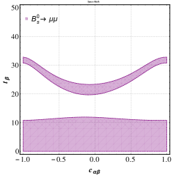
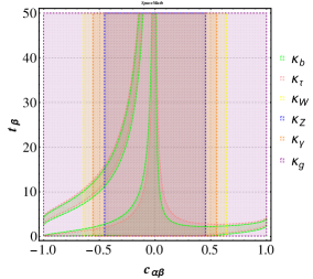
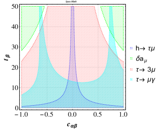
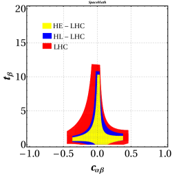
Figure 2: The shadowed areas represent the allowed regions in the plane $c_{\alpha\beta}$-$t_{\beta}$: (a) $B_{s}^{0}\to\mu^{+}\mu^{-}$, (b) Coupling modifiers $\kappa$-factors, (c) LFV processes and (d) Intersection of all allowed regions in which we show the cases for the LHC, HL-LHC and HE-LHC.

3.2 Constraint on $m_{H}$, $m_{A}$ and $m_{H^{\pm}}$

3.2.1 $m_{H}$ and $m_{A}$

The ATLAS and CMS collaborations presented results of a search for additional neutral Higgs bosons in the ditau decay channel ATLASCONF2017 ; Sirunyan:2018zut . The former of them searched through the process $gb\to\phi\to\tau\tau$, with $\phi=A,\,H$; figure 3 shows the Feynman diagram of this reaction. However, no evidence of any additional Higgs boson was observed. Nevertheless, upper limits on the production cross section $\sigma(gb\to\phi)$ times branching ratio $\mathcal{BR}(\phi\to\tau\tau)$ were imposed.

Figure 3: Feynman diagram of the production of $\phi$ in association with a bottom quark at LHC, with a subsequent decay into $\tau\tau$ pair.

In this work we focus on the particular case of the search carried out by the ATLAS collaboration.

In figure 4(a), we present the $\sigma(gb\to Hb)\times\mathcal{BR}(H\to\tau\tau)$ as a function of $m_{H}$ for illustrative values of $t_{\beta}=5,\,8,\,40$ and $c_{\alpha\beta}=0.05$. Figure 4(b) shows the same but as a function of $m_{A}$ and values for $t_{\beta}=8,\,30,\,40$. In both plots, the black points and red crosses represent the expected and observed values at 95$\%$ CL upper limits, respectively; while the green (yellow) band indicates the interval at $\pm 1\sigma$ ($\pm 2\sigma$) with respect to the expected value. We implement the Feynman rules in CalcHEP CalcHEP in order to evaluate $\sigma(gb\to\phi b)\times\mathcal{BR}(\phi\to\tau\tau)$.

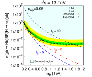
(a)

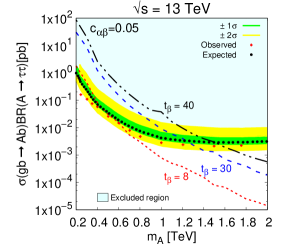
(b)

Figure 4: The observed and expected at 95$\%$ CL upper limits on the production cross section times ditau branching ratio for a scalar boson produced via $b$-associated production as a function of (a) the $\mathcal{CP}$-even mass for $t_{\beta}=$5, 8, 40 and (b) the $\mathcal{CP}$-odd mass for $t_{\beta}=$ 8, 30, 40. We take $c_{\alpha\beta}=0.05$.

From figure 4(a) we note that $m_{H}\lesssim 690$ GeV ($m_{H}\lesssim 510$ GeV) are excluded at 2$\sigma$ (1$\sigma$) for $t_{\beta}=8$, while for $t_{\beta}\lesssim 4$ the upper limit on $\sigma(gb\to\phi b)\times\mathcal{BR}(\phi\to\tau\tau)$ is easily accomplished. Although $t_{\beta}=$40 is discarded, as shown in figure 2, we include it to have an overview of the behavior of the model. On the other side, from figure 4(b), we observe that $m_{A}\lesssim 710$ GeV ($m_{H}\lesssim$ 610 GeV) are excluded at 2$\sigma$ (1$\sigma$) for $t_{\beta}=8$.

3.2.2 Constraint on the charged scalar mass $m_{H^{\pm}}$

The discovery of a charged scalar $H^{\pm}$ would constitute unambiguous evidence of new physics. Direct constraints can be obtained from collider searches for the production and decay of on-shell charged Higgs bosons. These limits are very robust and model-independent if the basic assumptions on the production and decay modes are satisfied Khachatryan:2015qxa ; Aad:2013hla ; Khachatryan:2015uua ; CMS:2016qoa . More recently the ATLAS collaboration reported a study on the charged Higgs boson produced either in top-quark decays or in association with a top quark. Subsequently the charged Higgs boson decays via $H^{\pm}\to\tau^{\pm}\nu_{\tau}$ with a center-of-mass energy of 13 TeV Aaboud:2018gjj . We analyze this process through the CalcHEP package, however, we find that this process is not a good way to impose a stringent bound on $m_{H^{\pm}}$.

Conversely, the decay $b\to s\gamma$ imposes stringent limits on $m_{H^{\pm}}$ because a new ingredient with respect to the SM contribution Chetyrkin:1996vx ; Adel:1993ah ; Ali:1995bi ; Greub:1996tg is the presence of the charged scalar boson coming from 2HDM-III which gives contributions to the Wilson coefficients of the effective theory as is shown in the Refs. Ciuchini:1997xe ; Misiak:2017bgg .

In figure 5 we show $R_{quark}$ at NLO in QCD as a function of the charged scalar boson mass for $t_{\beta}=2,5,10$, where $R_{quark}$ is defined as following:

$$R_{quark}=\frac{\Gamma(b\to X_{s}\gamma)}{\Gamma(b\to X_{c}e\nu_{e})}.$$ (41)

We observe that for $t_{\beta}=2$, the charged scalar boson mass $100\,\text{GeV}\lesssim m_{H^{\pm}}$ ($700\,\text{GeV}\lesssim m_{H^{\pm}}$) is excluded, at $2\sigma$ ($1\sigma$); while $t_{\beta}=10$ imposes a more restrictive lower bound $1.6\,\text{TeV}\lesssim m_{H^{\pm}}$ ($3.2\,\text{TeV}\lesssim m_{H^{\pm}}$) at $2\sigma$ ($1\sigma$).

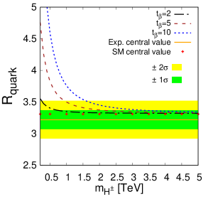
Figure 5: $R_{quark}$ at NLO in QCD as a function of the charged scalar boson mass for $t_{\beta}=$2, 5, 10. Solid line represents the experimental central value while red crosses indicate the theoretical SM central value. Green and yellow bands stand for 1$\sigma$ and 2$\sigma$, respectively. $R_{quark}$ is defined in the main text.

In summary, table 1 shows the values of the 2HDM-III parameters involved in the subsequent calculations.

Table 1: Values of the parameters used in the calculations.

Parameter	Values
$c_{\alpha\beta}$	0.05
$t_{\beta}$	0.1-8
$\chi_{\tau\mu}$	1
$m_{H}=m_{A}$	800 GeV

4 Search for the $h\to\tau\mu$ decay at future hadron colliders

We are interested in a possible evidence for the $h\to\tau\mu$ decay at future hadron collider. Thus, in this section we analyze the LFV process of the Higgs boson decaying into a $\tau\mu$ pair and its production at future hadron colliders via the gluon fusion mechanism. We first analyze the behavior of the branching ratio of the $h\to\tau\mu$ decay as a function of $t_{\beta}$ for $\chi_{\tau\mu}=0.1,\,0.5,\,1$ and $c_{\alpha\beta}=0.05$. Figure 6 shows the $\mathcal{BR}(h\to\tau\mu)$ as a function of $t_{\beta}$ including the upper limit on $\mathcal{BR}(h\to\tau\mu)$ reported by CMS and ATLAS collaborations Sirunyan:2017xzt ; ATLAS:2019icc .

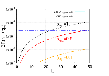
Figure 6: Branching ratio of the $h\to\tau\mu$ decay as a function of $t_{\beta}$ for $\chi_{\tau\mu}=0.1,\,0.5,\,1$. The horizontal line represents the upper limit on $\mathcal{BR}(h\to\tau\mu)$.

We analyze three scenarios that correspond to each of the future hadron colliders, namely:

• Scenario A (SA): HL-LHC at a center-of-mass energy of 14 TeV and integrated luminosities in the interval 0.3-3 ab^-1,

• Scenario B (SB): HE-LHC at a center-of-mass energy of 27 TeV and integrated luminosities in the range 0.3-12 ab^-1,

• Scenario C (SC): FCC-hh at a center-of-mass energy of 100 TeV and integrated luminosities from 10 to 30 ab^-1.

4.1 Number of signal and background events

Once the free model parameters were constrained in section 3, we now turn to evaluate the number of events produced of the signature $gg\to h\to\tau\mu$.

In figure 7 we present the $\sigma(gg\to h)\mathcal{BR}(h\to\tau\mu)$ as a function of $t_{\beta}$ (left axis) and the Events-$t_{\beta}$ plane (right axis) for scenarios SA, SB and SC. In all figures, the dark area represents the consistent region with allowed parameter space found in section 3 (see table 1). We observe that the maximum signal number of events ($\mathcal{N}_{\mathcal{S}}^{\textbf{SX}}$) produced are of the order of $\mathcal{N}_{\mathcal{S}}^{\textbf{SA}}=\mathcal{O}(10^{5})$, $\mathcal{N}_{\mathcal{S}}^{\textbf{SB}}=\mathcal{O}(10^{6})$, $\mathcal{N}_{\mathcal{S}}^{\textbf{SC}}=\mathcal{O}(10^{7})$, by considering $t_{\beta}=8$ and $\chi_{\tau\mu}=1$. Where we consider the most up-to-date constrains reported by LHC, in which a value for $t_{\beta}$ of up to 8 is allowed for $c_{\alpha\beta}=0.05$ (see figure 2).

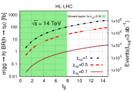
(a)

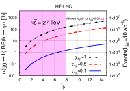
(b)

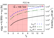
(c)

Figure 7: (a) Scenario SA, (b) Scenario SB, (c) Scenario SC. Left axis: $\sigma(gg\to h)\mathcal{BR}(h\to\tau\mu)$ as a function of $t_{\beta}$ for $\chi_{\tau\mu}$=0.1, 0.5, 1. Right axis: Events-$t_{\beta}$ plane. The dark area corresponds to the allowed region. See table 1.

4.2 Monte Carlo analysis

We will now analyze the signature of the decay $h\to\tau\mu$, with $\tau\mu=\tau^{-}\mu^{+}+\tau^{+}\mu^{-}$ and its potential SM background. The ATLAS and CMS collaborations ATLAShtaumu ; CMShtaumu searched two $\tau$ decay channels: electron decay $\tau\to e\nu_{\tau}\nu_{e}$ and hadron decay $\tau_{h}\mu$. In our analysis, we will concentrate on the electron decay. As far as our computation scheme is concerned, we first implement the relevant Feynman rules via LanHEP Semenov:2014rea for MadGraph5 MadGraphNLO , later it is interfaced with Pythia8 Sjostrand:2008vc and Delphes 3 delphes for detector simulations. Subsequently, we generate 10⁵ signal and background events, the last ones at NLO in QCD. We used CT10 parton distribution functions PDFs .

Signal and SM background processes

The signal and background processes are as following:

• SIGNAL: The signal is $gg\to h\to\tau\mu\to e\nu_{\tau}\nu_{e}\mu$. The electron channel must contain exactly two opposite-charged leptons, namely, one electron and one muon. Therefore, we search for the final state $e\mu$ plus missing energy due to neutrinos not detected.

• BACKGROUND: The main SM background arises from:

  1. Drell-Yan process, followed by the decay $Z\to\tau\tau\to e\nu_{\tau}\nu_{e}\mu\nu_{\tau}\nu_{\mu}$.

  2. $WW$ production with subsequent decays $W\to e\nu_{e}$ and $W\to\mu\nu_{\mu}$.

  3. $ZZ$ production, later decaying into $Z\to\tau\tau\to e\nu_{\tau}\nu_{e}\mu\nu_{\tau}\nu_{\mu}$ and $Z\to\nu\nu$.

Signal significance

The main kinematic cuts to isolate the signal are the collinear and transverse mass defined as following:

$$m_{\text{col}}(e\,\mu)=\frac{m_{\text{inv}}(e\,\mu)}{\sqrt{x}},\,\text{with}\,x=\frac{|\vec{P}_{T}^{e}|}{|\vec{P}_{T}^{e}|+\vec{E}_{T}^{\text{miss}}\cdot\vec{P}_{T}^{e}}$$ (42)

and

$$M_{T}^{\ell}=\sqrt{2|\vec{P}_{T}^{\ell}||\vec{E}_{T}^{\text{miss}}|(1-\cos\Delta\phi_{\vec{P}_{T}^{\ell}-\vec{E}_{T}^{\text{miss}}})}.$$ (43)

In figure 8 we show the distribution of collinear mass versus number of signal events for the scenarios (a) SA, (b) SB and (c) SC with integrated luminosities of 3, 12 and 30 ab^-1, respectively. In all scenarios we consider $t_{\beta}$= 5, 8.

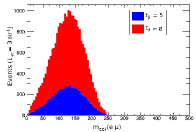
(a)

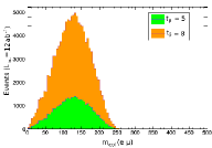
(b)

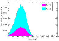
(c)

Figure 8: Distribution of the collinear mass versus number of signal events for scenarios (a) SA, (b) SB and (c) SC.

We use the package MadAnalysis5 MadAnalysis to analyze the kinematic distributions. Additional cuts applied both signal and background ATLAShtaumu ; CMShtaumu are shown in Table 2 for scenario SA. The kinematic cuts associated to scenarios SB and SC are available electronically in web_cuts . We also display the event number of the signal ($\mathcal{N}_{S}$) and background ($\mathcal{N}_{B}$) once the kinematic cuts were applied. The signal significance considered is defined as the ratio $\mathcal{N}_{S}/\sqrt{\mathcal{N}_{S}+\mathcal{N}_{B}}$. The efficiency of the cuts for the signal and background are: $\epsilon_{S}\approx 0.13$ and $\epsilon_{B}\approx 0.014$, respectively.

Table 2: Kinematic cuts applied to the signal and main SM background for scenario $\mathbf{SA}$, i.e, at HL-LHC with a center-of-mass energy $\sqrt{s}=14$ TeV and $\mathcal{L}_{\text{int}}=3$ ab^-1 for $t_{\beta}=8$.

Cut number	Cut	$\mathcal{N}_{S}$	$\mathcal{N}_{B}$	$\mathcal{N}_{S}/\sqrt{\mathcal{N}_{S}+\mathcal{N}_{B}}$
	Initial (no cuts)	$57665$	$200089020$	$4.08$
$1$	$|\eta^{e}|<2.3$	$25282$	$132346436$	$2.1975$
$2$	$|\eta^{\mu}|<2.1$	$16378$	$106936728$	$1.5837$
$3$	$0.1<\Delta R(e,\,\mu)$	$16355$	$106801230$	$1.5825$
$4$	$10<p_{T}(e)$	$15533$	$38846174$	$2.4817$
$5$	$20<p_{T}(\mu)$	$12119$	$20357367$	$2.6852$
$6$	$10<\text{MET}$	$11185.9$	$20086662$	$2.4952$
$7$	$100<m_{\text{col}}(e,\,\mu)<150$	$9645.1$	$9330510$	$3.1560$
$8$	$25<M_{T}(e)$	$8669.4$	$4827617$	$3.942$
$9$	$15<M_{T}(\mu)$	$7869$	$2867711$	$4.6404$

We find that at the LHC is not possible to claim for evidence of the decay $h\to\tau\mu$ achieving a signal significance about $1.46\sigma$ by considering its final integrated luminosity, 300 fb^-1. More promising results arise at HL-LHC in which a prediction of about $4.6\sigma$, once an integrated luminosity of 3 ab^-1 and $t_{\beta}=8$ are achieved. Meanwhile, at HE-LHC (FCC-hh) a potential discovery could be claimed with a signal significance of around $5.04\sigma$ ($\sim 5.43\sigma$) for an integrated luminosity of 9 ab^-1 and $t_{\beta}=6$ (15 ab^-1 and $t_{\beta}=3$). To illustrate the above, in figure 9 we present the signal significance as a function of $t_{\beta}$ for integrated luminosities associated with each scenario, namely:

• SA: from 0.3 ab^-1 at 3 ab^-1 for the HL-LHC,

• SB: from 3 ab^-1 at 12 ab^-1 for the HE-LHC,

• SC: from 10 ab^-1 at 30 ab^-1 for the FCC-hh.

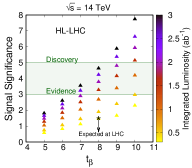
(a)

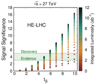
(b)

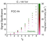
(c)

Figure 9: Signal significance as a function of $t_{\beta}$ and integrated luminosities associated to each scenario: (a) SA, (b) SB and (c) SC.

Finally, we present in figure 10 an overview of the signal significance as a function of the integrated luminosity for representative values of $t_{\beta}$.

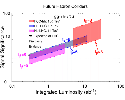
Figure 10: Signal significance as a function of the integrated luminosity for representative values of $t_{\beta}$.

5 Conclusions

In this article we have studied the LFV decay $h\to\tau\mu$ within the context of the 2HDM type III and we analyze its possible detectability at future super hadron colliders, namely, HL-LHC, HE-LHC and the FCC-hh.

We find the allowed model parameter space by considering the most up-to-date experimental measurements and later is used to evaluate the Higgs boson production cross section via the gluon fusion mechanism and the branching ratio of the $h\to\tau\mu$ decay.

A Monte Carlo analysis of the signal and its potential SM background was realized. We find that the closest evidence could arise at the HL-LHC with a prediction of the order of 4.66$\sigma$ for an integrated luminosity of 3 ab^-1 and $\tan\beta=8$. On the other hand, a potential discovery could be claimed at the HE-LHC (FCC-hh) with a signal significance about 5.046$\sigma$ (5.43$\sigma$) for an integrated luminosity of 3 ab^-1 and $\tan\beta=8$ (5 ab^-1 and $\tan\beta=4$).

If the decay considered in this research is observed in a future super hadron collider, then it will be a clear signal of physics BSM.

Appendix A Complementary formulas used in the analysis of the model parameter space

In this Appendix we present the analytical expressions in order to obtain the constraints on both diagonal and LFV couplings as is shown in Figure 2.

A.1 SM-like Higgs boson into $f_{i}\bar{f}_{j}$

We first start with the expression for the width decay of SM-like Higgs boson into fermion pair, which is given by:

$$\Gamma(h\to f_{i}\bar{f}_{j})=\frac{g^{2}_{hf_{i}\bar{f}_{j}}N_{c}m_{h}}{128\pi}\left(4-\left(\sqrt{\lambda_{f_{i}}}+\sqrt{\lambda_{f_{j}}}\right)^{2}\right)^{3/2}\left(4-\left(\sqrt{\lambda_{f_{i}}}-\sqrt{\lambda_{f_{j}}}\right)^{2}\right)^{1/2},$$ (44)

where $\lambda_{f_{k}}=4m_{f_{k}}^{2}/m_{h}^{2}$, with $k=i,\,j$; $N_{c}$ is the color number. In our case $g_{h\tau\mu}=\frac{c_{\alpha\beta}t_{\beta}}{\sqrt{2}s_{\beta}}\tilde{Y}_{\tau\mu}$ with $\tilde{Y}_{\tau\mu}=\frac{\sqrt{m_{\tau}m_{\mu}}}{\upsilon}\chi_{\tau\mu}$. We set $\chi_{\tau\mu}=1$.

A.2 Tau decays $\tau\to\mu\gamma$ and $\tau\to\mu\bar{\mu}\mu$

As far as the $\tau\to\mu\gamma$ decay is concerned, it arises at the one-loop level and receives contributions of $\phi=h,\,H,\,A$. Feynman diagrams for this process are displayed in figure 11(a). The decay width is given by:

$$\Gamma(\tau\to\mu\gamma)=\frac{\alpha m_{\tau}^{5}}{64\pi^{4}}\left(|A_{S}|^{2}+|A_{P}|^{2}\right),$$ (45)

where the $A_{S}$ and $A_{P}$ coefficients indicate the contribution from $A$ and $H$, respectively. In the limit of $g_{\phi\tau\tau}\gg g_{\phi\mu\mu}\gg g_{\phi ee}$ and $m_{\tau}\gg m_{\mu}\gg m_{e}$, they can be approximated as Harnik:2012pb

$$A_{S}=A_{P}\simeq\sum_{\phi=h,H_{F},A_{F}}\frac{g_{\phi\tau\tau}g_{\phi\mu\tau}}{12m_{\phi}^{2}}\left(3\ln\left(\frac{m_{\phi}^{2}}{m_{\tau}^{2}}\right)-4\right).$$ (46)

Two-loop contributions can be relevant, their expressions are reported in Harnik:2012pb , in our research we consider this contribution. The current experimental limit on the branching ratio is $\mathcal{BR}(\tau\to\mu\gamma)<4.4\times 10^{-8}$.

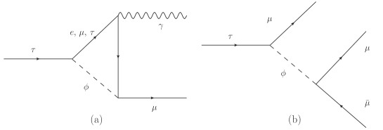
Figure 11: Feynman diagrams that contribute to (a) $\tau\to\mu\gamma$ and (b) $\tau\to\mu\bar{\mu}\mu$ decays with exchange of a scalar boson $\phi$. We omit both the bubble diagrams for the LFV decay $\tau\to\mu\gamma$, because only serve to cancel the ultraviolet divergences.

As for the $\tau\to\mu\bar{\mu}\mu$ decay, it receives contributions from $\phi$ as depicted in the Feynman diagram of Figure 11(b). The tree-level decay width can be approximated as

$$\Gamma(\tau\to\mu\bar{\mu}\mu) \simeq\frac{m_{\tau}^{5}}{256\pi^{3}}\Bigg{(}\frac{S_{h}^{2}}{m_{h}^{4}}+\frac{S_{H}^{2}}{m_{H}^{4}}+\frac{S_{H}^{2}}{m_{H}^{4}}+\frac{2S_{h}S_{H}}{m_{h}^{2}m_{H}^{2}}+\frac{2S_{A}}{3m_{A}^{2}}\left(\frac{S_{h}}{m_{h}^{2}}+\frac{S_{H}}{m_{H}}\right)\Bigg{)},$$ (47)

where $S_{\phi}=g_{\phi\mu\mu}g_{\phi\mu\tau}$. The upper bound on the branching ratio is $BR(\tau\to\mu\bar{\mu}\mu)<2.1\times 10^{-8}$ PDG .

A.3 Muon anomalous magnetic dipole moment

The muon AMDM also receives contributions from $\phi$, which are induced by a triangle diagram similar to the diagram of Figure 11(a) but with two external muons. The corresponding contribution can be approximated for $m_{\phi}\gg m_{l}$ as Harnik:2012pb

$$\delta a_{\mu}\sim\frac{m_{\mu}}{16\pi^{2}}\sum_{\phi=h,H,A}\sum_{l=\mu,\tau}\frac{m_{l}g_{\phi\mu l}^{2}}{m_{\phi}^{2}}\left(2\ln\left(\frac{m_{\phi}^{2}}{m_{l}^{2}}\right)-3\right),$$ (48)

where one must take into account the NP corrections to the $g_{h\mu\mu}$ coupling only. If $H$ and $A$ are too heavy, the dominant NP contribution would arise from the SM Higgs boson.

The discrepancy between the experimental value and the SM theoretical prediction is

$$\Delta a_{\mu}=a_{\mu}^{exp}-a_{\mu}^{SM}=(2.88\pm 0.63\pm 0.49)\times 10^{-9}.$$ (49)

Thus, the requirement that this discrepancy is accounted for by Eq. (48) leads to the bound $1.32\times 10^{-9}\leq\Delta a_{\mu}\leq 4.44\times 10^{-9}$ with $95\%$ C.L.

A.4 Decay $B_{s}^{0}\to\mu^{-}\mu^{+}$

$B_{s}^{0}$ meson decay into $\mu^{+}\mu^{-}$ pair is both interesting and stringent due to its sensitivity to constrain BSM theories. The SM theoretical prediction is $3.660\times 10^{-9}$ Beneke:2019slt while the experimental value is $(3.00\pm 0.6^{+0.3}_{-0.2})\times 10^{-9}$ PDG . In the context of the THDM-III, the decay $B_{s}^{0}\to\mu^{+}\mu^{-}$ is mediated by the SM-like Higgs boson, the heavy scalar $H$ and the pseudoscalar $A$ and it arises at tree level. Feynman diagram at the quark level is shown in Figure 12.

Figure 12: Feynman diagram for the decay $B_{s}^{0}\to\mu^{+}\mu^{-}$.

The branching ratio for this decay is given by Crivellin:2013wna

$$\begin{array}[]{ccl}\mathcal{BR}\left[B_{s}\rightarrow\mu^{+}\mu^{-}\right]&=&\frac{G_{F}^{4}M_{W}^{4}}{8\pi^{5}}\sqrt{1-4\frac{m_{\mu}^{2}}{M_{B_{s}}^{2}}}M_{B_{s}}f_{B_{s}}^{2}m_{\mu}^{2}\tau_{B_{s}}\\ &\times&\left[\left|\frac{M_{B_{s}}^{2}\left(C_{P}^{bs}-C_{P}^{\prime bs}\right)}{2\left(m_{b}+m_{s}\right)m_{\mu}}-\left(C_{A}^{bs}-C_{A}^{\prime bs}\right)\right|^{2}+\left|\frac{M_{B_{s}}^{2}\left(C_{S}^{bs}-C_{S}^{\prime bs}\right)}{2\left(m_{b}+m_{s}\right)m_{\mu}}\right|^{2}\times\left(1-4\frac{m_{\mu}^{2}}{m_{B_{s}}^{2}}\right)\right]\end{array}$$ (52)

$$\begin{array}[]{c}C_{S}^{q_{f}q_{i}}=\frac{\pi^{2}}{2G_{F}^{2}M_{W}^{2}}\sum_{k=1}^{3}\frac{1}{m_{H_{k}^{0}}^{2}}\left(\Gamma_{l_{B}l_{A}}^{LRH_{k}^{0}}+\Gamma_{l_{B}l_{A}}^{RLH_{k}^{0}}\right)\Gamma_{q_{f}q_{i}}^{RLH_{k}^{0}}\\ C_{P}^{q_{f}q_{i}}=\frac{\pi^{2}}{2G_{F}^{2}M_{W}^{2}}\sum_{k=1}^{3}\frac{1}{m_{H_{k}^{0}}^{2}}\left(\Gamma_{l_{B}l_{A}}^{LRH_{k}^{0}}-\Gamma_{l_{B}l_{A}}^{RLH_{k}^{0}}\right)\Gamma_{q_{f}q_{i}}^{RLH_{k}^{0}}\\ C_{S}^{\prime q_{f}q_{i}}=\frac{\pi^{2}}{2G_{F}^{2}M_{W}^{2}}\sum_{k=1}^{3}\frac{1}{m_{H_{k}^{0}}^{2}}\left(\Gamma_{l_{B}l_{A}}^{LRH_{k}^{0}}+\Gamma_{l_{B}l_{A}}^{RLH_{k}^{0}}\right)\Gamma_{q_{f}q_{i}}^{LRH_{k}^{0}}\\ C_{P}^{\prime q_{f}q_{i}}=\frac{\pi^{2}}{2G_{F}^{2}M_{W}^{2}}\sum_{k=1}^{3}\frac{1}{m_{H_{k}^{0}}^{2}}\left(\Gamma_{l_{B}l_{A}}^{LRH_{k}^{0}}-\Gamma_{l_{B}l_{A}}^{RLH_{k}^{0}}\right)\Gamma_{q_{f}q_{i}}^{LRH_{k}^{0}}\end{array}$$ (57)

References

- (1) M. Raidal et al, Flavour physics of leptons and dipole moments, Eur. Phys. J. C57 (2008) 13-182. doi: 10.140/epjc/s10052-008-0715-2, arXiv: 0801.1826
- (2) Q.R. Ahmad et al., [SNO Collab.], Phys. Rev. Lett. 87, 071301 (2001); Q.R. Ahmad et al., [SNO Collab.], Phys. Rev. Lett. 89, 011301 (2002).
- (3) K. Eguchi et al., [KamLAND Collab.], Phys. Rev. Lett. 90, 021802 (2003); T. Araki et al., [KamLAND Collab.], Phys. Rev. Lett. 94, 081801 (2005).
- (4) Y. Fukuda et al., [Super-Kamiokande Collab.], Phys. Rev. Lett. 81, 1562 (1998); Y. Ashie et al., [Super-Kamiokande Collab.], Phys. Rev. Lett. 93, 101801 (2004).
- (5) M.H. Ahn et al., [K2K Collab.], Phys. Rev. D74, 072003 (2006).
- (6) B. Pontecorvo, Zh. Eksp. Teor. Fiz. 33, 549 (1957) and 34, 247 (1958).
- (7) Z. Maki, M. Nakagawa, and S. Sakata, Prog. Theor. Phys. 28, 870 (1962).
- (8) K. Hayasaka et al., Phys. Lett. B 687 (2010) 139 [arXiv:1001.3221 [hep-ex]].
- (9) U. Bellgardt et al. [SINDRUM Collaboration], Nucl. Phys. B 299 (1988) 1.
- (10) A. M. Baldini et al. [MEG Collaboration], Eur. Phys. J. C 76 (2016) no.8, 434 [arXiv:1605.05081 [hep-ex]].
- (11) B. Aubertet al.[BaBar Collaboration], Phys. Rev. Lett.104(2010) 021802 [arXiv:0908.2381[hep-ex]].
- (12) J. L. Diaz-Cruz and J. J. Toscano, Phys. Rev. D 62, 116005 (2000).
- (13) T. Han and D. Marfatia, Phys. Rev. Lett. 86, 1442 (2001).
- (14) K. A. Assamagan, A. Deandrea, and P.-A. Delsart, Phys. Rev. D 67, 035001 (2003).
- (15) J. L. Diaz-Cruz, J. High Energy Phys. 05 (2003) 036.
- (16) E. Arganda, A. M. Curiel, M. J. Herrero, and D. Temes, Phys. Rev. D 71, 035011 (2005).
- (17) A. Brignole and A. Rossi, Nucl. Phys. B701, 3 (2004).
- (18) J. L. Diaz-Cruz, D. K. Ghosh, and S. Moretti, Phys. Lett. B 679, 376 (2009).
- (19) S. Chamorro-Solano, A. Moyotl, and M. A. Pérez, arXiv: 1707.00100.
- (20) S. Chamorro-Solano, A. Moyotl, and M. A. Perez, J. Phys.: Conf. Ser. 761, 012051 (2016).
- (21) A. Lami and P. Roig, Phys. Rev. D 94, 056001 (2016).
- (22) Arroyo-Urena MA, Bolanos A, Diaz-Cruz JL, Hernandez-Tome G, Tavares-Velasco G (2018) Searching for LFV Flavondecays at hadron colliders 1801.00839
- (23) G. Aad et al. (ATLAS Collaboration), Phys. Lett. B 716, 1 (2012).
- (24) S. Chatrchyan et al. (CMS Collaboration), Phys. Lett. B 716, 30 (2012).
- (25) G. Aad et al. [ATLAS], Phys. Lett. B 800, 135069 (2020) doi:10.1016/j.physletb.2019.135069 [arXiv:1907.06131 [hep-ex]].
- (26) A. M. Sirunyan et al. [CMS], JHEP 03, 103 (2020) doi:10.1007/JHEP03(2020)103 [arXiv:1911.10267 [hep-ex]].
- (27) G. Apollinari, O. Brning, T. Nakamoto, and L. Rossi, CERN Yellow Report pp. 1–19 (2015), 1705.08830.
- (28) M. Benedikt and F. Zimmermann, Proton colliders at the energy frontier, Nucl. Instrum. Meth. A 907 (2018) 200 [arXiv:1803.09723].
- (29) N. Arkani-Hamed, T. Han, M. Mangano and L.-T. Wang, Physics opportunities of a 100 TeV proton-proton collider, Phys. Rept. 652 (2016) 1 [arXiv:1511.06495].
- (30) J. F. Gunion, H. E. Haber, G. L. Kane, and S. Dawson, The Higgs Hunter?S Guide (Addison-Wesley, Reading, MA, 2000).
- (31) T. P. Cheng and M. Sher, Phys. Rev. D 35, 3484 (1987).
- (32) H. E. Haber, G. L. Kane, and T. Sterling, Nucl. Phys. B161, 493 (1979).
- (33) H. Fritzsch, Nucl. Phys. B155, 189 (1979).
- (34) J. F. Gunion and H. E. Haber, Phys. Rev. D 67, 075019 (2003) doi:10.1103/PhysRevD.67.075019 [hep-ph/0207010].
- (35) J. Hernńdez-Sńchez, S. Moretti, R. Noriega-Papaqui and A. Rosado, JHEP1307, 044 (2013)[arXiv:1212.6818 [hep-ph]].
- (36) H. Fritzsch and Z. -Z. Xing, Phys. Lett. B, 353: 114 (1995) [hep-ph/9502297].
- (37) G. C. Branco, D. Emmanuel-Costa and R. Gonzalez Felipe, Phys. Lett. B, 477: 147 (2000) [hep-ph/9911418]
- (38) J. Lorenzo Díaz-Cruz, Rev. Mex. Fis. 65, no. 5, 419 (2019) doi:10.31349/RevMexFis.65.419 [arXiv:1904.06878 [hep-ph]].
- (39) J.L. Díaz-Cruz, R. Noriega-Papaqui and A. Rosado, Mass matrix ansatz and lepton flavor violation in the THDM-III, Phys. Rev. D 69 (2004) 095002 [hep-ph/0401194] [ IN SPIRE ].
- (40) M.A. Arroyo-Urena, J.L. Díaz-Cruz, E. Díaz and J.A. Orduz-Ducuara, Flavor violating Higgs signals in the texturized two-Higgs doublet model (THDM-Tx), Chin. Phys. C 40 (2016) 123103 [arXiv:1306.2343].
- (41) R. Gaitán, R. Martinez, J. H. M. de Oca and E. A. Garcés, Phys. Rev. D 98, no.3, 035031 (2018) doi:10.1103/PhysRevD.98.035031 [arXiv:1710.04262 [hep-ph]].
- (42) T. P. Cheng and M. Sher, Phys. Rev. D 35, 3484 (1987). doi:10.1103/PhysRevD.35.3484
- (43) ATLAS Collaboration, CERN Report No. ATLAS-CONF-2017-055, 2017.
- (44) A. M. Sirunyan et al. [CMS Collaboration], JHEP 1809, 007 (2018) doi:10.1007/JHEP09(2018)007 [arXiv:1803.06553 [hep-ex]].
- (45) M. Aaboud et al. [ATLAS Collaboration], JHEP 1809, 139 (2018) doi:10.1007/JHEP09(2018)139 [arXiv:1807.07915 [hep-ex]].
- (46) K. G. Chetyrkin, M. Misiak and M. Munz, Phys. Lett. B 400, 206 (1997) Erratum: [Phys. Lett. B 425, 414 (1998)] doi:10.1016/S0370-2693(97)00324-9 [hep-ph/9612313].
- (47) K. Adel and Y. P. Yao, Phys. Rev. D 49, 4945 (1994) doi:10.1103/PhysRevD.49.4945 [hep-ph/9308349].
- (48) A. Ali and C. Greub, Phys. Lett. B 361, 146 (1995) doi:10.1016/0370-2693(95)01118-A [hep-ph/9506374].
- (49) C. Greub, T. Hurth and D. Wyler, Phys. Rev. D 54, 3350 (1996) doi:10.1103/PhysRevD.54.3350 [hep-ph/9603404].
- (50) M. Ciuchini, G. Degrassi, P. Gambino and G. F. Giudice, Nucl. Phys. B 527, 21 (1998) doi:10.1016/S0550-3213(98)00244-2 [hep-ph/9710335].
- (51) M. Misiak and M. Steinhauser, Eur. Phys. J. C 77, no. 3, 201 (2017) doi:10.1140/epjc/s10052-017-4776-y [arXiv:1702.04571 [hep-ph]].
- (52) The ATLAS collaboration [ATLAS Collaboration], ATLAS-CONF-2018-031.
- (53) A. M. Sirunyan et al. [CMS Collaboration], Eur. Phys. J. C 79, no. 5, 421 (2019) doi:10.1140/epjc/s10052-019-6909-y [arXiv:1809.10733 [hep-ex]].
- (54) M. Tanabashi et al. (Particle Data Group), Phys. Rev. D 98, 030001 (2018)
- (55) A. M. Sirunyan et al. [CMS Collaboration], JHEP 1806, 001 (2018) doi:10.1007/JHEP06(2018)001 [arXiv:1712.07173 [hep-ex]].
- (56) The ATLAS collaboration [ATLAS Collaboration], ATLAS-CONF-2019-013.
- (57) M. Cepeda,et. al., CERN Yellow Rep. Monogr. 7, 221-584 (2019) doi:10.23731/CYRM-2019-007.221 [arXiv:1902.00134 [hep-ph]].
- (58) The ATLAS collaboration [ATLAS Collaboration], ATL-PHYS-PUB-2018-005
- (59) M.A. Arroyo-Ureña and T.A. Valencia-Pérez, SpaceMath 1.0. package for beyond the standard model parameter space searches, arXiv:2008.00564 [hep-ph].
- (60) A. Belyaev, N. D. Christensen, and A. Pukhov, Comput. Phys. Commun. 184, 1729 (2013).
- (61) V. Khachatryan et al. [CMS Collaboration], JHEP 1511, 018 (2015) doi:10.1007/JHEP11(2015)018 [arXiv:1508.07774 [hep-ex]].
- (62) G. Aad et al. [ATLAS Collaboration], Eur. Phys. J. C 73, no. 6, 2465 (2013) doi:10.1140/epjc/s10052-013-2465-z [arXiv:1302.3694 [hep-ex]].
- (63) V. Khachatryan et al. [CMS Collaboration], JHEP 1512, 178 (2015) doi:10.1007/JHEP12(2015)178 [arXiv:1510.04252 [hep-ex]].
- (64) CMS Collaboration [CMS Collaboration], CMS-PAS-HIG-16-030.
- (65) G. Aad et al. (ATLAS Collaboration), Eur. Phys. J. C 77, 70 (2017).
- (66) V. Khachatryan et al. (CMS Collaboration), Phys. Lett. B 749, 337 (2015).
- (67) A. Semenov, Comput. Phys. Commun. 201, 167 (2016) doi:10.1016/j.cpc.2016.01.003 [arXiv:1412.5016 [physics.comp-ph]].
- (68) J. Alwall, M. Herquet, F. Maltoni, O. Mattelaer, and T.Stelzer, J. High Energy Phys. 06 (2011) 128.
- (69) T. Sjostrand, doi:10.3204/DESY-PROC-2009-02/41 arXiv:0809.0303 [hep-ph].
- (70) J. de Favereau, C. Delaere, P. Demin, A. Giammanco, V. Lemaitre, A. Mertens, and M. Selvaggi, J. High Energy Phys. 02 (2014) 057.
- (71) J. Gao, M. Guzzi, J. Huston, H.-L. Lai, Z. Li, P. Nadolsky, J. Pumplin, D. Stump, and C. P. Yuan, Phys. Rev. D 89, 033009 (2014).
- (72) E. Conte, B. Fuks, and G. Serret, Comput. Phys. Commun. 184, 222 (2013).
- (73) https://drive.google.com/open?id=1LRixxTVcGpfyRmj321Y8PRPESWclBNES
- (74) R. Harnik, J. Kopp and J. Zupan, JHEP 1303, 026 (2013) doi:10.1007/JHEP03(2013)026 [arXiv:1209.1397 [hep-ph]].
- (75) M. Beneke, C. Bobeth and R. Szafron, JHEP 10 (2019), 232 doi:10.1007/JHEP10(2019)232 [arXiv:1908.07011 [hep-ph]].
- (76) A. Crivellin, A. Kokulu and C. Greub, Phys. Rev. D 87, no.9, 094031 (2013) doi:10.1103/PhysRevD.87.094031 [arXiv:1303.5877 [hep-ph]].