Dating the Break in High-dimensional Data

Abstract

This paper is concerned with estimation and inference for the location of a change point in the mean of independent high-dimensional data. Our change point location estimator maximizes a new U-statistic based objective function, and its convergence rate and asymptotic distribution after suitable centering and normalization are obtained under mild assumptions. Our estimator turns out to have better efficiency as compared to the least squares based counterpart in the literature. Based on the asymptotic theory, we construct a confidence interval by plugging in consistent estimates of several quantities in the normalization. We also provide a bootstrap-based confidence interval and state its asymptotic validity under suitable conditions. Through simulation studies, we demonstrate favorable finite sample performance of the new change point location estimator as compared to its least squares based counterpart, and our bootstrap-based confidence intervals, as compared to several existing competitors. The asymptotic theory based on high-dimensional U-statistic is substantially different from those developed in the literature and is of independent interest.

, and

t1Runmin Wang is Ph.D. Candidate and Xiaofeng Shao is Professor, Department of Statistics, University of Illinois at Urbana-Champaign, Champaign, IL 61820 (e-mail: rwang52, xshao@illinois.edu).

1 Introduction

Advances in science and technology have led to an explosion of data of high dimension. Examples of high-dimensional data include fMRI imaging data in neuroscience, genomic data in biological science, panel time series data from economics and finance, and spatio-temporal data from climate science, among others. Often statisticians assume some kind of homogeneity assumptions in analyzing such data, such as i.i.d. (independent and identically distributed) or stationarity with weak serial dependence for a sequence of high-dimensional data. The validity of methodology they develop can be sensitive with respect to such assumptions. In this paper, we shall focus on a particular type of non-homogeneity, a change point in the mean of an otherwise i.i.d. sequence of high-dimensional data. That is, we assume that our observed data follows the one-change point model,

$$CP1:~{}X_{t}=\mu_{t}+Z_{t},t=1,\cdots,n,$$

where $Z_{t}$ are i.i.d. $p$-dimensional data with zero mean, and $\mu_{t}=\mu_{1}{\bf 1}(1\leq t\leq k_{0})+(\mu_{1}+\delta){\bf 1}(k_{0}+1\leq t\leq n)$. In this model, both parameters $\delta$ and $k_{0}=n\tau_{0},$ where $\tau_{0}\in(0,1)$, are unknown. Our main goal is to provide a new estimator of break point $\tau_{0}$ and a confidence interval, which works in the high-dimensional setting that allows $p>>n$ and also dependence within $p$ components. To achieve this, we develop a new $U$-statistic based objective function and propose to use its maximizer as our location estimator. Under some mild assumptions, this new estimator is shown to be consistent with suitable convergence rate and asymptotic distribution upon centering and normalization. It is also shown to be superior to the least squares based counterpart in Bai, (2010) and Bhattacharjee et al., (2019), for some specific models of interest. Furthermore, we provide a bootstrap-based confidence interval that can be adaptive to the magnitude of change, theoretically justified and works well in finite sample.

The literature on change point testing and estimation for high-dimensional data has been growing at a fast pace lately, as stimulated by the practical needs of analyzing high-dimensional data with change points. From the viewpoint of mathematical statistics, the high dimensionality can bring substantial methodological and theoretical challenges, as many classical estimation and testing procedures developed for low-dimensional data may not work in the high-dimensional setting. This also brings interesting opportunities to the mathematical statistics community, as there is a great need to develop new estimation and testing methods that can accommodate high dimensionality and dependence within components and over time. As there is a vast literature on retrospective change point testing and estimation in the low-dimensional setting, we refer the readers to several excellent review papers and books, see e.g., Csörgő and Horváth, (1997), Perron, (2006), and Aue and Horváth, (2013) for many references.

Below we shall provide a brief review of the more recent literature on high-dimensional change point inference. For testing a change point in the mean of high-dimensional data, Horváth and Hušková, (2012) considered an $l_{2}$ aggregation of one-dimensional CUSUM statistics, which targets at dense alternative. For a sequence of Gaussian vectors, Enikeeva and Harchaoui, (2019) proposed a new test to detect the presence of a change point in mean and established the detection boundary in different regimes that allow the dimension to approach the infinity. Their test was formed on the basis of a combination of a linear statistic and a scan statistic, which can capture both sparse and dense alternatives, but their critical values were obtained under strong Gaussian and independent components assumptions. Cho and Fryzlewicz, (2015) proposed a sparse binary segmentation algorithm for detecting multiple change points in the second order structure of a high-dimensional time series, by aggregating the low-dimensional CUSUM statistics that pass a certain threshold. Cho, (2016) developed a double CUSUM statistic that can be viewed as an interesting extension of the ideas in Enikeeva and Harchaoui, (2019) and Cho and Fryzlewicz, (2015), and her test was shown to be consistent in estimating the change points with binary segmentation allowing for dependence over time and across cross-sections. Jirak, (2015) considered an $l_{\infty}$ aggregation of CUSUM statistics, which aims for sparse alternatives. The “INSPECT” method proposed in Wang and Samworth, (2018) was based on sparse projection method for a single change point and it has been extended to multiple change point estimation by combining with the wild binary segmentation [Fryzlewicz, (2014)]. Wang et al., (2019) proposed a U-statistic based approach to test for change points in independent high-dimensional data via self-normalization, as an extension of Shao and Zhang, (2010), and also provided an segmentation algorithm by using the wild binary segmentation. Chen et al., (2019) proposed an $l_{\infty}$ based statistic to test for change points in trends for high-dimensional time series with a consistent estimator of the long-run covariance matrix. Also see Yu and Chen, (2017) for another $l_{\infty}$ based test for one change point alternative in mean.

For the estimation and confidence interval construction of the break point $\tau_{0}$ (or $k_{0}$), there have been many papers written on this topic when the dimension $p$ is low and fixed; see early work by Hinkley, (1970), Hinkley, (1972), Picard, (1985), Bhattacharya, (1987), Yao, (1987) and Bai, (1994), among others. There have been extensions to the change point problems in linear regression and multivariate time series; see Bai, 1997b , Bai and Perron, (1998) and Bai et al., (1998), but all these works focused on the low-dimensional case. Relatively little is done in the high-dimensional setting. Bai, (2010) considered a least square estimator for the change point location in the panel data with independent cross section units and weak dependence over time, and obtained the asymptotic distribution of break date estimator. Recently Bhattacharjee et al., (2019) extended the least squares method in Bai, (2010) to high-dimensional time series and their setting allowed for both cross-sectional and serial dependence. Bai, (2010), Bhattacharjee et al., (2019) and Chen et al., (2019) provided an asymptotic distribution for the suitable centered and normalized break date estimator and constructed a confidence interval for the break date. Since both Bai, (2010) and Bhattacharjee et al., (2019) tackled the one-change point model, we shall provide a detailed comparison with these two papers in theory and numerical simulations later. It is worth noting that the temporal independence assumption is often assumed in change point analysis for genomic data; see Zhang et al., (2010), Jeng et al., (2010) and Zhang and Siegmund, (2012) among others.

A word on notations. For a vector $a\in R^{p}$, $\|a\|$ is the Euclidean norm. For a matrix $A\in R^{p\times p}$, denote $\|A\|$ and $\|A\|_{F}$ as the spectral norm and the Frobenious norm respectively, and denote $tr(A)$ as the trace of $A$. Define $\lfloor\cdot\rfloor$ as the floor function. We use $cum(X_{1},X_{2},...,X_{n})$ to represent the joint cumulants of random variables $X_{1},...,X_{n}$. Throughout the paper, all asymptotic results are stated under the regime $n\wedge p\rightarrow\infty$.

The rest of the article is organized as follows. Section 2 presents a new method to estimate $\tau_{0}$ based on the U-statistic, and contains all the asymptotic results. Section 3 introduces several methods of constructing confidence intervals for $\tau_{0}$, including a bootstrap-based method and its theoretical justification. Section 4 gathers all simulation results. Section 5 concludes and mentions a few future research topics. All technical proofs are relegated to Sections 6 and 7.

2 Estimation Method and Asymptotic Theory

Under the one-change point model CP1: $X_{t}=\mu_{1}{\bf 1}(1\leq t\leq k_{0})+(\mu_{1}+\delta){\bf 1}(k_{0}+1\leq t\leq n)+Z_{t},$ for $t=1,2,...,n$, where $\{Z_{t}\}_{t=1}^{n}$ are $p$-dimensional i.i.d. random vectors with mean $0$ and variance matrix $\Sigma$. Here we follow the convention in the change point literature and denote the true unknown location of the change point as $k_{0}=\tau_{0}n$, $\tau_{0}\in(0,1)$, i.e., $k_{0}$ is a fixed positive fraction of the sample size $n$. Without loss of generality, assume $\mu_{1}=0$ as our estimation method is invariant to the value of $\mu_{1}$. For notational convenience, we shall not use the double-array notation $X_{t,n}$, $Z_{t,n}$, etc.

Consider the statistic $G_{n}(k)$ such that for all $k=2,3,...,n-2$,

$$G_{n}(k)=\frac{1}{k(n-k)}\sum_{i_{1},i_{2}=1,i_{1}\neq i_{2}}^{k}\sum_{j_{1},j_{2}=k+1,j_{1}\neq j_{2}}^{n}(X_{i_{1}}-X_{j_{1}})^{T}(X_{i_{2}}-X_{j_{2}}).$$

We define

$$\hat{k}_{U}=\operatornamewithlimits{argmax}_{k=2,...,n-2}G_{n}(k)$$

as the estimate of the change point location (or break date) $k_{0}$. This is a natural estimator since $\mathbb{E}[G_{n}(k)]$ achieves its maximum when $k$ is the true change point location, as shown in the lemma below. We define $\hat{\tau}_{U}=\hat{k}_{U}/n$ as the estimate of the relative position $\tau_{0}$. Let $a_{n}=n^{2}\|\delta\|^{4}/\|\Sigma\|_{F}^{2}$, which is the rate of convergence for $\hat{\tau}_{U}$ to be shown later.

Lemma 2.1.

$\mathbb{E}[G_{n}(k)]=(k-1)(n-k_{0})(n-k_{0}-1)\|\delta\|^{2}/(n-k)$ when $k\leq k_{0}$ and $\mathbb{E}[G_{n}(k)]=(n-k-1)k_{0}(k_{0}-1)\|\delta\|^{2}/k$ when $k\geq k_{0}$. Hence $\mathbb{E}[G_{n}(k)]$ achieves its maximum at $k=k_{0}$.

In Bai, (2010), the location of change point is estimated by minimizing a least squares criterion, that is

$$\hat{k}_{LS}=\operatornamewithlimits{argmin}_{k=1,2,...,n-1}SSR(k):=\sum_{i=1}^{k}\|X_{i}-\bar{X}_{1:k}\|^{2}+\sum_{i=k+1}^{n}\|X_{i}-\bar{X}_{(k+1):n}\|^{2},$$ (2.1)

where $\bar{X}_{a:b}$ is the sample average based on the subsample $\{X_{a},X_{a+1},...,X_{b}\}$, for any $1\leq a\leq b\leq n$. The least squares method is natural in the low-dimensional setting; see Bai, (1994), Bai, 1997a , Bai and Perron, (1998), among others in either one break or multiple break model with or without covariates.

In the high-dimensional setting, the use of U-statistic was first initiated by Chen and Qin, (2010) in the two sample testing for the equality of means. Recently, Wang et al., (2019) extended the U-statistic based approach to high-dimensional change point testing, coupled with the idea of self-normalization [Shao, (2010), Shao and Zhang, (2010), Shao, (2015)]. In this paper, we further advance the U-statistic based approach to the estimation of change point location in the one change-point model, and our proof techniques are substantially different from that in Bai, (2010) and Bhattacharjee et al., (2019) due to the use of a different objective function, and also very different from that in Wang et al., (2019) due to the focus on the asymptotic behavior of the estimator. We shall compare the performance of our location estimator with the least squares based counterpart in theory and simulations later.

To investigate the asymptotic properties of our location estimator $\hat{\tau}_{U}$, we introduce the following assumptions.

Assumption 2.2.

1. $tr(\Sigma^{4})=o(\|\Sigma\|_{F}^{4})$.

2. There exists a positive constant $C$ independent of $n$ such that

   $$\sum_{j_{1},...j_{h}=1}^{p}cum^{2}(Z_{0,j_{1}},...Z_{0,j_{h}})\leq C\|\Sigma\|_{F}^{h},$$

   for $h=2,3,4,5,6$.

3. $\sqrt{\delta^{T}\Sigma\delta}=o\left(\sqrt{n}\|\delta\|^{2}/{\sqrt{a_{n}}}\right)=o({\|\Sigma\|_{F}}/{\sqrt{n}})$.

4. $a_{n}=o(n)$ and $\log(n)=o(a_{n})$.

Remark 2.3 (Discussion of Assumptions).

Assumption 2.2(a) and 2.2(b) are identical to the assumptions used in Wang et al., (2019), where a U-statistic based approach was developed for change point testing in the high-dimensional setting. These assumptions essentially impose weak dependence among the $p$ components, which can be verified for AR type correlation or models with banded componentwise dependence, but are violated when the variance-covariance matrix is compound symmetric; see detailed discussion in Remark 3.2 of Wang et al., (2019).

Assumption 2.2(c) guarantees the change point signal dominates the noise in the U-statistic and it is equivalent to $\frac{n\delta^{T}\Sigma\delta}{\|\Sigma\|_{F}^{2}}=o(1)$. In the special case $\Sigma=I_{p}$, it is reduced to $\|\delta\|^{2}=o(p/n)$. Assumption 2.2(d) defines the particular regime we are considering. Note that when $a_{n}=o(1)$, the U-statistic based test developed in Wang et al., (2019) delivers trivial power asymptotically; see Theorem 3.5 therein. This suggests that the restriction $\log(n)=o(a_{n})$ is almost necessary in order for $\tau_{0}$ to be consistently estimated; see Theorem 2.4 below. The condition $a_{n}=o(n)$ represents a particular regime under which a meaningful asymptotic distribution for the suitably centered and normalized location estimator can be obtained. In the case that $\Sigma=I_{p}$, Assumption 2.2(d) is equivalent to $\{\log(n)p\}^{1/2}/n=o(\|\delta\|^{2})$ and $\|\delta\|^{2}=o((p/n)^{1/2})$ We offer more discussions about what happens in other regimes later; see Theorem 2.8.

Theorem 2.4 (Rate of Convergence).

Suppose that Assumptions 2.2 hold. Then for any $\epsilon>0$, there exists $M>0$, such that for large enough $n$,

$$P(\hat{k}_{U}\in\Omega_{n}(M))<\epsilon,$$

where $\Omega_{n}(M)=\{k:|k-k_{0}|>nM/a_{n}\}$.

Theorem 2.4 implies that $\hat{\tau}_{U}$ is a rate-$a_{n}$ consistent estimator for $\tau_{0}$. Following the conventional argument in studying the limiting behavior of $M$-estimator [Van der Vaart and Wellner, (1996)], we reparametrize and define $\gamma=a_{n}(\tau-\tau_{0})$. Then

$$\hat{\gamma}_{n}:=a_{n}(\hat{\tau}_{U}-\tau_{0})=\operatornamewithlimits{argmin}_{\gamma\in R}~{}L_{n}(\gamma;\tau_{0})$$

where $L_{n}(\gamma;\tau_{0}):=\frac{\sqrt{2}\sqrt{a_{n}}}{n\|\Sigma\|_{F}}\{G_{n}(n\tau_{0})-G_{n}(\lfloor n\tau_{0}+n\gamma/a_{n}\rfloor)\}.$

To proceed, we define

$$G_{n}^{Z}(k)=\frac{1}{k(n-k)}\sum_{i_{1},i_{2}=1,i_{1}\neq i_{2}}^{k}\sum_{j_{1},j_{2}=k+1,j_{1}\neq j_{2}}^{n}(Z_{i_{1}}-Z_{j_{1}})^{T}(Z_{i_{2}}-Z_{j_{2}})$$

as an analog of $G_{n}(k)$. Let $\l_{\infty}([-M,M])$ denote the set of essentially bounded measurable functions on $[-M,M]$.

Theorem 2.5.

Under the Assumptions 2.2(a)-2.2(b), for any $b_{n}\rightarrow\infty$ and $b_{n}=o(n)$,

$$H_{n}(\gamma):=\frac{\sqrt{2}\sqrt{b_{n}}}{n\|\Sigma\|_{F}}\left\{G_{n}^{Z}(\lfloor n\tau_{0}\rfloor)-G_{n}^{Z}(\lfloor n\tau_{0}+n\gamma/b_{n}\rfloor)\right\}\rightsquigarrow\frac{2\sqrt{2}}{\sqrt{\tau_{0}(1-\tau_{0})}}W^{*}{(\gamma)}$$

in $l_{\infty}([-M,M])$ for any fixed $M>0$, where $W^{*}(\gamma)$ is a two-sided Brownian motion. That is, when $\gamma<0$, $W^{*}(\gamma)=W_{1}(-\gamma)$ and when $\gamma\geq 0$, $W^{*}(\gamma)=W_{2}(\gamma)$, where $W_{1},W_{2}$ are independent standard Brownian motions defined on $[0,+\infty)$.

Theorem 2.5 gives a process convergence result for the properly normalized increment of the process $G_{n}^{Z}(\cdot)$ around the true change point in a shrinking neighborhood. By directly applying argmax continuous mapping theorem [Theorem 3.2.2, Van der Vaart and Wellner, (1996)], we can get the following corollary.

Corollary 2.6 (Asymptotic Distribution).

Under Assumptions 2.2, we can show that for any $M>0$,

$$L_{n}(\gamma;\tau_{0})\rightsquigarrow L(\gamma;\tau_{0}):=\sqrt{2}|\gamma|+\frac{2\sqrt{2}}{\sqrt{\tau_{0}(1-\tau_{0})}}W^{*}(\gamma)$$

in $l_{\infty}([-M,M])$. Consequently,

$$a_{n}(\hat{\tau}_{U}-\tau_{0})\overset{\mathcal{D}}{\rightarrow}\xi(\tau_{0}):=\operatornamewithlimits{argmin}_{\gamma\in(-\infty,\infty)}L(\gamma;\tau_{0})$$

Remark 2.7 (Discussion of $\xi(\tau_{0})$).

In fact, the distribution of $\xi({\tau_{0}})$ has been well studied in the literature. According to Proposition 1 in Stryhn, (1996), the probability density function of $\xi{(\tau_{0})}$, denoted as $f(t)$, is

$$f(t)=\frac{3}{2}\tau_{0}(1-\tau_{0})e^{\tau_{0}(1-\tau_{0})|t|}\Phi\left(-\frac{3}{2}\sqrt{\tau_{0}(1-\tau_{0})|t|}\right)-\frac{1}{2}\tau_{0}(1-\tau_{0})\Phi\left(-\frac{1}{2}\sqrt{\tau_{0}(1-\tau_{0})|t|}\right),$$

where $\Phi(\cdot)$ is the cumulative distribution function of a standard normal random variable. It is straightforward to see that $f(t)$ is symmetric, i.e. $f(t)=f(-t)$, for all $t\in\mathbb{R}$, and the densities of $\xi(\tau_{0})$ and $\xi(1-\tau_{0})$ are identical. Furthermore $f(t)$ achieves its unique maximum at $t=0$ and $f(0)=\tau_{0}(1-\tau_{0})/2$. In addition, the tail of the distribution is exponential and $Var(\xi(\tau_{0}))\propto(\tau_{0}(1-\tau_{0}))^{-2}$.

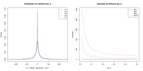
Figure 1: Density plot and quantile plot for different values of $\tau_{0}$

To approximate the distribution of $\xi(\tau_{0})$ and its critical values, we approximate the standard Brownian motion by standardized sum of i.i.d. standard normal random variables, and generate $10^{5}$ Monte-Carlo replicates of $\xi(\tau_{0})$ for $\tau_{0}=0.01,...,0.99$. Then we plot their densities and critical values over $\tau_{0}\in[0.01,0.5]$ in Figure 1.

Please insert Figure 1 here!

From Figure 1, we see that as $\tau_{0}$ moves from $0.5$ to $0.1$, the density is less concentrated around $0$, indicating the relative difficulty of accurately estimating $\tau_{0}$ when $\tau_{0}$ is close to $0$ or $1$. Correspondingly, the critical calues increase as $\tau_{0}$ goes from $0.5$ to $0.01$.

If Assumptions 2.2(a), 2.2(b) and 2.2(c) hold, there are indeed three regimes that correspond to different rates of $a_{n}$. Given $a_{n}/\log(n)\rightarrow\infty$, if $a_{n}/n\rightarrow 0$, this situation is covered by Corollary 2.6. There are two more regimes, under which the behavior of our estimator is discussed in the following theorem.

Theorem 2.8.

Under Assumptions 2.2(a) and 2.2(b),

1. $a_{n}/n\rightarrow c\in(0,\infty)$: if Assumption 2.2(c) also holds, our change point location estimator still works in the sense that

   $$\hat{k}_{U}-k_{0}\overset{\mathcal{D}}{\rightarrow}\operatornamewithlimits{argmin}_{\gamma\in\mathbb{Z}}L(\gamma,\tau_{0})$$

   and $(\hat{k}_{U}-k_{0})=O_{p}(1)$.

2. $a_{n}/n\rightarrow\infty$: if $\sqrt{\delta^{T}\Sigma\delta}=o(\|\delta\|^{2})$, then we have $P(\hat{k}_{U}\neq k_{0})\rightarrow 0$.

We shall offer some comparison with the methods, theory and assumptions in Bai, (2010) and Bhattacharjee et al., (2019), as the latter two papers both addressed change point estimation in the one change point model. To elaborate the differences, we shall separate our discussions into several categories as follows.

1: Model assumptions and estimation methods. Although all three papers assumed one change point in mean for a sequence of high-dimensional observations, there are substantial differences. In particular, Bai, (2010) assumed componentise independence (or so-called cross-sectional independence) but allowed weak temporal dependence for each series; Bhattacharjee et al., (2019) relaxed the cross-sectional independence assumption in Bai, (2010) and allowed weak dependence over time and also within components. By contrast, we require the data to be independent over time but allow for weak componentwise dependence. This makes a direct comparison of the three papers quite challenging, so we shall focus on some specific cases only. Note that in both Bai, (2010) and Bhattacharjee et al., (2019), an infinite order vector moving average process (i.e., VMA($\infty$)) was assumed.

Denote the break date estimator in Bai, (2010) as $\hat{\tau}_{LS}=\hat{k}_{LS}/n$, which is obtained as the minimizer of a least squares criterion, see (2.1). Let $\hat{\tau}_{BBM}$ denote the estimator used in Bhattacharjee et al., (2019) where the minimum is taken over $k\in[\lfloor c^{*}n\rfloor,\lfloor(1-c^{*})n\rfloor]$ for some prespecified $c^{*}\in(0,0.5)$. It should be expected that $P(\hat{\tau}_{LS}\not=\hat{\tau}_{BBM})\rightarrow 0$ if $\tau_{0}\in(c^{*},1-c^{*})$. By contrast, our break date estimator $\hat{\tau}_{U}$ is the maximizer of a new U-statistic based objective function.

2: Asymptotic framework, regimes and technical assumptions. In Bai, (2010), he studied two asymptotic frameworks, $n$ fixed and $n\rightarrow\infty$ as $p\rightarrow\infty$ (Bai, (2010) used $N$ for our $p$, and $T$ for our $n$ in his paper). We shall only focus on a comparison with his result in the latter case, i.e., $\min(n,p)\rightarrow\infty$. To make a fair comparison, we shall discuss the case for which both theories are expected to work, which is the case of cross-sectional and temporal independence. To facilitate the comparison, we further assume $\Sigma=I_{p}$. Under this condition, our Assumptions 2.2(a) and 2.2(b) are automatically satisfied.

Under the assumption that $\|\delta\|^{2}\rightarrow\infty$, Theorem 3.2 in Bai, (2010) stated that if $\log(\log(n))p/n\rightarrow 0$, then $P(\hat{k}_{LS}\neq k_{0})\rightarrow 0$. This corresponds to our third regime, where $a_{n}/n\rightarrow\infty$ and $\sqrt{\delta^{T}\Sigma\delta}=\|\delta\|=o(\|\delta\|^{2})$, which implies that $P(\hat{k}_{U}\neq k_{0})\rightarrow 0$ as well, see Theorem 2.8. Under the assumption that $\|\delta\|^{2}\rightarrow C\in(0,\infty)$, $\log(\log(n))p/n\rightarrow 0$ and $\delta^{T}\Sigma\delta\rightarrow C^{\prime}\in(0,\infty)$, Theorem 4.2 of Bai, (2010) asserted the asymptotic distribution for $\hat{k}_{LS}-k_{0}$. These assumptions imply $a_{n}/n\rightarrow\infty$, however $\sqrt{\delta^{T}\Sigma\delta}$ is no longer $o(\|\delta\|^{2})$. This does not belong to any one of our three regimes stated early. But interestingly, under this specific setting our estimator $\hat{k}_{U}$ converge to the same distribution as $\hat{k}_{LS}$, and we shall prove this result below in Proposition 2.9.

In addition to these two cases, our theory also uncovers an important and interesting regime Bai, (2010) did not consider, that is $a_{n}=o(n)$. In this case, as we showed earlier, there is a very nice interplay between the order of $\|\delta\|^{2}$ and $(n,p)$ that allows $p$ to diverge faster than $n$, such that there is an asymptotic distribution for $a_{n}(\hat{\tau}_{U}-\tau_{0})$. Thus in a sense, our theory is more complete than the one in Bai, (2010) for this specific model.

Bhattacharjee et al., (2019) extended the method and theory in Bai, (2010) to accommodate both cross-sectional and temporal (serial) dependence. They also used the $VMA(\infty)$ model with a mean shift, but to accommodate the cross-sectional dependence, many additional assumptions were imposed. For example, Bhattacharjee et al., (2019) required finite fourth moment, whereas Bai, (2010) did not. Also they required that the number of nonzero elements in $\delta$ cannot vary with $n$; see assumption (A4) in their paper. Such requirement is not needed in our technical analysis. Different from the conditions used in Bai, (2010), there is no explicit restriction on the relative relationship between $p$ and $n$ in Bhattacharjee et al., (2019). See Remark 2.10 for additional explanations.

3: Convergence rates and efficiency comparison. To compare with the theory in Bhattacharjee et al., (2019), we shall focus on the following model,

$$X_{t}=\delta\boldsymbol{1}\{t>k_{0}\}+A\epsilon_{t},\qquad t=1,2,...,n,$$

where $\{\epsilon_{t}\}$ are i.i.d. $p$-dimensional random vectors with zero mean and identity covariance matrix, $A$ is $p\times p$ real-valued matrix and $\delta\in\mathbb{R}^{p}$ is the vector of mean change. In our setting, we can set $A=\Sigma^{1/2}$, and hence $\Sigma=AA^{T}$. This model allows cross-sectional dependence but enforces temporal independence, so is included in our framework. It can also be viewed as a special case of the VMA$(\infty)$ model with a mean shift in Bhattacharjee et al., (2019) as basically we let $A_{j}=A$ when $j=0$ and $A_{j}=0$ for $j\geq 1$ in their VMA representation. According to Theorem 2.1 and Theorem 2.2 of Bhattacharjee et al., (2019), to guarantee the consistency of $\hat{\tau}_{BBM}$, the signal-to-noise ratio (SNR) has to grow to infinity, i.e. $SNR=\frac{n\|\delta\|^{2}}{p\|A\|^{2}}\rightarrow\infty.$ Under this condition, $\hat{\tau}_{BBM}$ is consistent with the rate of convergence $a_{n}^{(BBM)}=p\times SNR=n\|\delta\|^{2}/\|A\|^{2}$. Notice that the rate of convergence for $\hat{\tau}_{U}$ is $a_{n}=n^{2}\|\delta\|^{4}/\|\Sigma\|_{F}^{2}$. When $SNR\rightarrow\infty$,

$$\frac{a_{n}}{a_{n}^{(BBM)}}=\frac{n^{2}\|\delta\|^{4}}{\|\Sigma\|_{F}^{2}}\cdot\frac{\|A\|^{2}}{n\|\delta\|^{2}}=\frac{n\|\delta\|^{2}}{p\|A\|^{2}}\cdot\frac{p\|A\|^{4}}{\|\Sigma\|_{F}^{2}}\geq SNR\cdot\frac{p\|A\|^{4}}{p\|AA^{T}\|^{2}}\geq SNR\rightarrow\infty,$$

where the first inequality is due to the fact that $\|\Sigma\|_{F}^{2}\leq p\|\Sigma\|^{2}$, and the second inequality in the above derivation is because $\|AA^{T}\|\leq\|A\|^{2}$. This is a significant finding as it means that for the above specific model, if assumptions for both methods are satisfied, the convergence rate corresponding to our U-statistic based estimator is faster.

To ensure the consistency of our break point estimator $\hat{\tau}_{U}$, we also require a signal-to-noise condition, i.e., $a_{n}/\log(n)\rightarrow\infty$. Since $a_{n}\geq a_{n}^{(BBM)}SNR=p\cdot SNR^{2}$ as shown in the above display, $a_{n}/\log(n)\rightarrow\infty$ provided that (a) $p=O(\log(n))$ and $SNR\rightarrow\infty$ or (b) $\log(n)=o(p)$ and $SNR$ is fixed. This implies that our U-statistic based estimator can be consistent with suitable convergence rate under a weaker signal setting as compared to the least squares counterpart. In other words, $\hat{\tau}_{U}$ is a consistent estimator of $\tau_{0}$ under much weaker conditions than $\hat{\tau}_{BBM}$. We shall provide some theoretical explanation for this phenomenon in Remark 2.10.

Furthermore, similar to our Theorem 2.8 where we have described two additional regimes according to different orders of $(a_{n}/n)$, the asymptotic behavior of $\hat{\tau}_{BBM}$ also has three regimes depending on the order of $(a_{n}^{(BBM)}/n)$. Under certain assumptions, if $a_{n}^{(BBM)}/n\rightarrow\infty$, the asymptotic distribution of $\hat{k}_{BBM}-k_{0}$ is degenerate at zero. In this case, since $a_{n}/a_{n}^{(BBM)}\geq SNR\rightarrow\infty$, the limiting distribution of $\hat{k}_{U}-k_{0}$ is also degenerate at zero, as $a_{n}^{(BBM)}/n\rightarrow\infty$ implies that $a_{n}/n\rightarrow\infty$ under the assumption that $SNR\rightarrow\infty$. This suggests that the regime that corresponds to the degenerate limiting distribution for $\hat{k}_{BBM}$ is well included in the regime that corresponds to degenerate limiting distribution for $\hat{k}_{U}$.

Of course, the results in Bhattacharjee et al., (2019) are generally applicable to the temporal dependent case, so the slower convergence rate relative to our estimator, which is tailed to the independent high-dimensional data, is probably not surprising. Nevertheless, it shows that our new location estimator can bring substantial efficiency gain relative to the least squares based counterpart in the case of independent high-dimensional data.

Proposition 2.9.

Both estimators $\hat{k}_{LS}$ and $\hat{k}_{U}$ converge to the same limiting distribution if

1. $\Sigma=I_{p}$,

2. $\|\delta\|^{2}\rightarrow c\in(0,\infty)$

3. $\log(\log(n))p/n\rightarrow 0$.

Remark 2.10.

The main reason why Bai, (2010) only provided theories under the setting $p=o(n)$ is that the objective function he used is least squares based and it contains extra diagonal terms that need to be controlled under certain restriction on the growth rate of $p$ as a function of $n$. To be specific, as we showed in the proof of Proposition 2.9, the first three terms of $SSR(k)-SSR(k_{0})$ (i.e., $I_{j}$, $j=1,2,3$) are of form $\sum_{i=a}^{b}Z_{i}^{T}Z_{i}$ (up to a multiplication constant) for some $1\leq a<b\leq n$ that needs to be of smaller magnitude than the leading terms in his theoretical derivation, so these three terms have to be controlled under the assumption $p=o(n)$ since if $n=o(p)$ the three diagonal terms can dominate the others. In contrast, in our U-statistic based objective function, we essentially remove the diagonal terms, so no growth rate assumption as $p=o(n)$ is required and we are able to cover the “large $p$ small $n$” case automatically.

The advantage of U-statistic over the least squares counterpart was in fact stated in Chen and Qin, (2010) under the two sample testing framework. Compared to an important early paper by Bai and Saranadasa, (1996), which involves a least squares term in the test statistic, Chen and Qin, (2010) used a U-statistic to remove the diagonal terms, which are not useful in the testing and incur unnecessary growth rate constraints in the theoretical analysis. Therefore in a sense, our U-statistic based approach inherits this advantage from Chen and Qin, (2010) and allows our theory to cover the interesting ”large $p$ small $n$” case (i.e., $p>>n$).

It is worth noting that Bhattacharjee et al., (2019) considered almost the same estimator as Bai, (2010) but extended the theory to a more general setting including the large $p$ small $n$ case. In Bhattacharjee et al., (2019), the control of diagonal terms in the least squares based objective function was explicitly done by imposing some extra conditions. In particular their condition (A4) was used to control the order of the diagonal terms. However, these additional assumptions seem hard to verify in practice. In comparison, our four assumptions are relatively more transparent and interpretable.

3 Confidence interval construction

Given the asymptotic theory presented in Section 2, we shall first describe a way of constructing a confidence interval for $\tau$ based on asymptotic approximation. Note that the normalizing constant $a_{n}$ depends on two unknown quantities, $\Delta=\|\delta\|^{2}$ and $\|\Sigma\|_{F}^{2}$. Fortunately, their consistent estimators have been provided by Chen and Qin, (2010) in the two sample testing context, and we can easily adapt them to our setting. Algorithm 1 describes the procedure for the plug-in approach below.

1. Estimate $k_{0}$: $\hat{k}_{U}=\operatornamewithlimits{argmax}_{k}G_{n}(k)$.

2. Estimate $\Delta=\|\delta\|^{2}$ : $\widehat{\Delta}=\frac{1}{(\hat{k}_{U}-1)(n-\hat{k}_{U}-1)}G_{n}(\hat{k}_{U})$.

3. Estimate $\|\Sigma\|_{F}^{2}$ : $\widehat{\|\Sigma\|_{F}^{2}}(\hat{k}_{U})$.

4. Estimate $a_{n}$: $\hat{a}_{n}=n^{2}\widehat{\Delta}^{2}/\widehat{\|\Sigma\|_{F}^{2}}(\hat{k}_{U})$.

5. $(1-\alpha)$ confidence interval for $\tau_{0}$: $[\hat{\tau}_{U}-q_{1-\alpha/2}(\xi(\hat{\tau}_{U}))/\hat{a}_{n},\hat{\tau}_{U}-q_{\alpha/2}(\xi(\hat{\tau}_{U}))/\hat{a}_{n}]$, where $q_{\alpha}(\xi({\tau}))$ denotes the $\alpha$-quantile of the distribution of $\xi({\tau})$.

Algorithm 1 Algorithm for constructing a confidence interval for $\tau_{0}$

In the Algorithm 1, we have used the jackknife type estimator $\widehat{\|\Sigma\|_{F}^{2}}(\hat{k}_{U})$ introduced in Chen and Qin (2010), to estimate $\|\Sigma\|_{F}^{2}$, i.e.,

$$\widehat{\|\Sigma\|_{F}^{2}}(\hat{k}_{U})=(\hat{k}_{U}(n-\hat{k}_{U}))^{-1}tr \left\{\sum_{i=1}^{\hat{k}_{U}}(X_{i}-\bar{X}_{(1:\hat{k}_{U},i)})(X_{i}-\bar{X}_{(1:\hat{k}_{U},i)})^{T}\right.$$

$$\left.\cdot\sum_{j=\hat{k}_{U}+1}^{n}(X_{j}-\bar{X}_{(\hat{k}_{U}+1:n,j)})(X_{j}-\bar{X}_{(\hat{k}_{U}+1:n,j)})^{T}\right\},$$

where $\bar{X}_{(a:b,i)}$ is the sample average of $X_{a},...,X_{b}$ excluding $X_{i}$.This slightly differs from the one used in Chen and Qin, (2010) in that we removed two terms that correspond to the two double sums within the pre-break sample and post-break sample. Simulation suggests that there is little impact on the coverage and length of intervals.

After preliminary simulations, we realize that there is considerable amount of coverage error for the above plug-in based confidence interval since this only covers the regime described in Corollary 2.6. There can be other regimes which have different convergence rates and in reality we may not be able to know which regime the data generating process falls into. This motivates us to propose the following bootstrap-based interval.

1. Estimate $k_{0}$ by $\hat{k}_{U}=\operatornamewithlimits{argmax}_{k}G_{n}(k)$ and $\hat{\tau}_{U}=\hat{k}_{U}/n$.

2. Estimate $\Delta$ by $\widehat{\Delta}=\frac{1}{(\hat{k}_{U}-1)(n-\hat{k}_{U}-1)}G_{n}(\hat{k}_{U})$, and let $\hat{\delta}=\boldsymbol{1}_{p}\sqrt{\widehat{\Delta}/p}$,where $\boldsymbol{1}_{p}$ is a $p$-dimensional vector with all elements equal to 1.

3. Estimate $\Sigma$ by some positive semi-definite estimator $\hat{\Sigma}_{X}$.

4. Generate random vectors $\epsilon_{1}$,…,$\epsilon_{n}$ in $\mathbb{R}^{p}$ from the distribution $\mathcal{N}(0,\hat{\Sigma}_{X})$.

5. Generate ${X}_{t}^{*}=\epsilon_{t}$ if $t\leq\hat{k}_{U}$ and ${X}_{t}^{*}=\hat{\delta}+\epsilon_{t}$ if $t>\hat{k}_{U}$.

6. Calculate the bootstrap estimate $\hat{k}_{U}^{*}$ by $\hat{k}_{U}^{*}=\operatornamewithlimits{argmax}_{k=2,...,n-2}G_{n}^{(X^{*})}(k),$ where $G_{n}^{(X^{*})}(k)$ denotes the value of $G_{n}(k)$ calculated based on $\{X_{t}^{*}\}$, and calculate the bootstrap estimate of the proportion by $\hat{\tau}_{U}^{*}=\hat{k}_{U}^{*}/n$.

7. Repeat step 4-6 for $B$ times to generate $\hat{\tau}^{*}_{U,1}$,…,$\hat{\tau}^{*}_{U,B}$, and 95% bootstrap CI for $\tau_{0}$ is $[\hat{\tau}_{U}-q^{*}_{0.975},\hat{\tau}_{U}-q^{*}_{0.025}]$, where $q^{*}_{0.025}$ and $q^{*}_{0.975}$ are the sample $2.5\%$ and $97.5\%$ quantiles for $\{\hat{\tau}^{*}_{U,i}-\hat{\tau}_{U}\}_{i=1}^{B}$.

Algorithm 2 Bootstrap algorithm for constructing a confidence interval for $\tau_{0}$

In Algorithm 2 we consider to use a uniform vector with squared norm equal to $\widehat{\Delta}$ to estimate the mean change vector, regardless of the sparsity of the truth $\delta$. The reason why this works is because the limiting distribution only depends on the norm of the mean change, not the vector of the mean change itself. To verify this we have also tried variants of the above algorithm by imposing different sparsity on $\hat{\delta}$ while maintaining the same norm, the finite sample performance turns out to be stable.

Theorem 3.1 (Bootstrap Consistency).

Suppose Assumption 2.2 holds. Further, we assume that

1. $tr({\hat{\Sigma}_{X}}^{4})/\|\hat{\Sigma}_{X}\|_{F}^{4}=o_{p}(1)$,

2. $\|\hat{\Sigma}_{X}\|=o_{p}(\max(n{\|\delta\|}^{2}/a_{n},\|\delta\|^{2}))$,

3. $\hat{a}_{n}/a_{n}\rightarrow_{p}1$.

Given the data, the conditional distribution of $\{a_{n}(\hat{\tau}_{U}^{*}-\hat{\tau}_{U})\}$ weakly converges to that of $\xi(\tau_{0})$ in probability, i.e.

$$a_{n}(\hat{\tau}_{U}^{*}-\hat{\tau}_{U})\overset{\mathcal{D}}{\rightarrow}\xi(\tau_{0})\text{ in P}.$$

Thus the bootstrap interval described in Algorithm 2 has desired coverage probability asymptotically, i.e.

$$P(\tau_{0}\in[\hat{\tau}_{U}-q^{*}_{1-\alpha/2},\hat{\tau}_{U}-q^{*}_{\alpha/2}])\rightarrow 1-\alpha.$$

Remark 3.2.

For the other two regimes besides the regime covered by Assumption 2.2, the bootstrap estimator $\hat{\tau}_{U}^{*}-\hat{\tau}_{U}$ has the same asymptotic behavior as $\hat{\tau}_{U}-\tau_{0}$ if the three conditions in the above theorem are satisfied. The proof is very similar to the proof of Theorem 3.1 so we skip the details. The verification of the two conditions (a) and (b) in Theorem 3.1 depend on what type of positive definite estimator $\hat{\Sigma}_{X}$ we adopt, and it requires a case-by-case analysis. Hence details are omitted.

Remark 3.3.

Bhattacharjee et al., (2019) required a stronger signal-to-noise condition for the bootstrap consistency result. Specifically, instead of the $SNR\rightarrow\infty$, they required $SNR\text{-}ADAP=\frac{n\|\delta\|^{2}}{p\log(p)\|A\|^{2}}\rightarrow\infty$. By contrast, the requirement for the signal-to-noise ratio in our bootstrap consistency result is identical to that for the consistency of our original estimator [cf. Theorem 2.5], which is $a_{n}/\log(n)\rightarrow\infty$.

4 Simulation studies

In this section, we study the finite sample performance of our proposed estimator and confidence intervals. We consider the single change point model (CP1) with the change point located at $n\tau_{0}$, i.e.

$$X_{t}=\delta\boldsymbol{1}\{t>n\tau_{0}\}+\epsilon_{t},\qquad t=1,2,...,n,$$ (4.1)

where $\{\epsilon_{t}\}$ are i.i.d. multivariate normal random vectors with mean zero and covariance $\Sigma$, $\delta$ is the mean change vector, and $\tau_{0}=0.2$ or $0.5$. To study the impact of componentwise dependence on the performance, we include four different models for $\Sigma$: (1) Identity (ID: $\Sigma=I_{p}$); (2) AR(1) (AR: $\Sigma(i,j)=0.8^{|i-j|}$); (3) Banded (BD: $\Sigma(i.j)=0.5^{|i-j|}\boldsymbol{1}\{|i-j|<=2\}$); (4) Compound Symmetric (CS: $\Sigma=0.5I_{p}+0.5\boldsymbol{1}\boldsymbol{1}^{T}$).

The sample size $n$ is chosen from $\{50,100,200\}$ and the dimension $p$ is chosen from $\{50,150\}$. Furthermore we consider two cases for the sparsity of $\delta$. One is dense change where $\delta$ is formed by $p$ i.i.d. random values generated from Uniform distribution $Unif[-0.5,0.5]$. The other is sparse change, where we first generate a $p$-dimensional random vector by the same procedure as what we have done for dense change and record its norm as $\|\delta\|$, and then generate $\delta=\|\delta\|(1/\sqrt{5},1/\sqrt{5},1/\sqrt{5},1/\sqrt{5},1/\sqrt{5},0,...,0)^{T}$ as the sparse vector. We fix $\delta$ for all Monte-Carlo replicates with the same $(n,p)$ combination.

We conduct two simulation studies under the above settings to evaluate the performance of the point estimators and confidence intervals, and we comment on the results below for these two studies respectively.

4.1 Finite sample performance of location estimators

We examine the finite sample performance of the location estimators, including our U-statistic based estimator (denoted as $\hat{\tau}_{U}$) and the least squares based estimator described in Bai, (2010) (denoted as $\hat{\tau}_{LS}$) by $20000$ Monte-Carlo replicates. The bias, variance and mean squared error (MSE) are summarized in Table 1 for $\tau_{0}=0.2$ and in Table 2 for $\tau_{0}=0.5$. As we can observe, $\hat{\tau}_{U}$ outperforms $\hat{\tau}_{LS}$ for almost all settings in terms of the MSE. There are two settings for $\tau_{0}=0.2$ with banded covariance structure ($(n,p)=(200,50)$ for sparse change and $(n,p)=(100,150)$ for dense change), where $\hat{\tau}_{U}$ has slightly larger MSE, and this could be due to random Monte Carlo errors. As we break the MSE criterion into (squared) bias and variance, we spot an interesting pattern. The biases for $\hat{\tau}_{U}$ and $\hat{\tau}_{LS}$ are mostly comparable, with no one dominating the other. The advantage of $\hat{\tau}_{U}$ in MSE is mostly attributed to its smaller variance, which may be explained by the usage of a U-statistic based objective function, as U-statistic has the well-known minimal variance property in estimation.

It can also be seen that when comparing the results for $\tau_{0}=0.2$ and $\tau_{0}=0.5$, there are substantially smaller bias and variance for all settings when $\tau_{0}=0.5$, which is consistent with our intuition that estimation is easier when $\tau_{0}=0.5$. Additionally, both methods exhibit a larger MSE for the compound symmetric case, as compared to other covariance structures. This is not surprising since the compound symmetric covariance matrix corresponds to strong componentwise dependence and violates the weak cross-sectional dependence assumptions necessary for both methods. Nevertheless, as sample size gets larger, the MSE gets smaller for all cases. A direct comparison between the dense change and the sparse charge shows that the results for both cases are very similar for all combinations of $(n,p)$ and models. This is quite reasonable since the performance of both methods essentially depends on the $l_{2}$ norm of the mean change, which we hold at the same level. Thus the sparsity of the mean change is not the critical factor in determining the finite sample performance of both estimators. Overall, our new estimator enjoys the efficiency gain over the least squares counterpart in almost all settings and should be preferred in the high-dimensional environment.

4.2 Finite sample performance of confidence intervals

In this section we evaluate the finite sample performance for confidence intervals. For each setting, we generate 3000 Monte-Carlo replicates and construct 7 different 95% confidence intervals for $\tau_{0}$ including:

1. Oracle U-statistic based CI ($U_{1}$): Constructed by Algorithm 1 with the true value for $a_{n}$ replacing $\hat{a}_{n}$.

2. U-statistic based CI ($U_{2}$): Constructed by Algorithm 1.

3. U-statistic based parametric bootstrap I ($U_{3}$): Constructed by modifying Algorithm 4. We estimate the location by $\hat{\tau}_{U}$, and follow steps 2-5 to generate bootstrap samples. For each bootstrap sample we used our U-statistic based method instead of least squares based method to estimate the location.

4. U-statistic based parametric bootstrap II ($U_{4}$): Constructed by Algorithm 2.

5. U-statistic based nonparametric bootstrap ($U_{5}$): We sample with replacement based on the pre-break sample and post-break sample separately to generate bootstrap data, where the break date is estimated by $\hat{\tau}_{U}$. The break date for the bootstrap sample is estimated by our method.

6. CI in Bai, (2010) ($LS_{1}$): Constructed by Algorithm 3.

7. Adaptive CI in Bhattacharjee et al., (2019) ($LS_{2}$): Constructed by Algorithm 4, which is a modified version of the one in Bhattacharjee et al., (2019) due to the temporal independence model we assume here. This main difference between this one and $U_{3}$ is that the least squares based approach was used for the break date estimation for both original and bootstrap sample, whereas the U-statistic based approach was used in the construction of $U_{3}$.

One thing worth pointing out is that in Algorithm 4, Bhattacharjee et al., (2019) originally used banded autocovariance matrix to generate bootstrap samples. However we found during our simulation that the banded covariance matrix may not be positive semi-definite and the sample covariance matrix itself is not a good estimate when the dimension is high. To solve this issue, we use the R package ”PDSCE” to get a positive definite estimate for the high-dimensional covariance matrix. Specifically, denote $S$ as the sample covariance matrix and $R$ as the sample correlation matrix. Denote $S^{+}$ as the diagonal matrix with the same diagonal as $S$ and $S^{-}=S-S^{+}$. Then the correlation matrix estimator is constructed as

$$\hat{\Theta}=\operatornamewithlimits{argmin}_{\Theta\succ 0}(\|\Theta-R\|_{F}^{2}/2-\lambda_{1}\log|\Theta|+\lambda_{2}|\Theta^{-}|_{1}),$$

where $\lambda_{1}$ is a fixed small positive constant, $\lambda_{2}$ is a non-negative tuning parameter, $|\cdot|$ is the determinant and $|\cdot|_{1}$ is the $l_{1}$ norm of the vectorized matrix. The tuning parameters are selected via a default cross-validation step in “PDSCE”. Then the estimated covariance matrix is constructed as $\hat{\Sigma}=(S^{+})^{1/2}\hat{\Theta}(S^{+})^{1/2}$. See Rothman, (2012) for more details about this methodology. Note that this is the covariance matrix estimate we used for our Algorithms 2 and 4, i.e., in the construction of $U_{3},U_{4}$ and $LS_{2}$.

The results are summarized in Tables 3-6. We calculate the sample coverage probability as well as the average length for each CI. Each table corresponds to a particular covariance model with all results for both sparse and dense changes, all combinations of $(n,p)$s and two cases $\tau_{0}=0.2,0.5$. It is apparent for some combinations of $(n,p)$, the coverages for all seven intervals are far below the nominal coverage level $95\%$, indicating the difficulty of constructing an interval with proper coverage, especially when $n$ is small and the dependence among components is strong.

The three intervals ($U_{1}$, $U_{2}$ and $LS_{1}$) are based on asymptotic approximation, which seem quite coarse as all these intervals exhibit serious undercoverage. It appears that in most cases $U_{1}$ and $U_{2}$ have better coverage than $LS_{1}$ when $p>n$ but have worse coverage than $LS_{1}$ when $p<n$, which is consistent with the asymptotic theory. Note that the undercoverage for $U_{1}$ and $U_{2}$ are tied to the fact that we always use $a_{n}$ for $U_{1}$ and $\hat{a}_{n}$ for $U_{2}$ as the rate of convergence, which is only correct for our regime $a_{n}/n\rightarrow 0$. However for other regimes the rates of convergence can be slower than $a_{n}$. This leads to an undercoverage. For the same reason, $LS_{1}$ fails to achieve the desired coverage probability since the theory is only valid for a specific regime and requires the cross-sectional independence.

The four bootstrap-based intervals ($U_{3}$, $U_{4}$, $U_{5}$ and $LS_{2}$) have overall almost uniform better coverages than the three counterparts based on asymptotic approximation. Among these four intervals, the ranking appears to be (in the order of preferences) $U_{4}>U_{5}>U_{3}>LS_{2}$. We can see that $U_{4}$ and $U_{5}$ have very comparable results for all settings. Both have about 95% coverage probability even for small $(n,p)$ when $\tau_{0}=0.5$. When $\tau_{0}=0.2$, the problem gets harder but they can still have a desired coverage when $n$ and $p$ are large, sometimes even too conservative. We have no theoretical justification for the nonparametric bootstrap procedure yet, but the simulation results are quite encouraging. We have also tried variants of $U_{4}$ by using a sparse estimate of $\delta$ and keeping the same $l_{2}$ norm, the results turn out to be similar to what we have here.

As a comparison, $LS_{2}$ is another least squares based interval and it has better coverage comparing to $LS_{1}$ by using a bootstrap procedure. But it still cannot achieve the desired confidence level for most settings when $\tau_{0}=0.2$. When $\tau_{0}=0.5$, it has decent coverage probability when the sample size is large. As we have discussed before, the rate of convergence of our estimator is faster than the least squares based estimator. Hence our methods ($U_{3}$, $U_{4}$ and $U_{5}$) can achieve the desired coverage with smaller $(n,p)$. Furthermore we observe that for large $p$ small $n$ situation, our methods still provide a good coverage whereas $LS_{2}$ cannot. This may be related to the fact that our methods work for both $n/p\rightarrow\infty$ and $n/p\rightarrow 0$ in theory, but the least squares based method only works for the case $p<<n$. Note that a higher coverage probability is usually associated with a longer interval.

Among other observations, we mention that for the same setting, the results for $\tau_{0}=0.5$ are always comparable or better than the results (in terms of more coverage and shorter interval length) for $\tau_{0}=0.2$ due to the fact the estimation problem for $\tau_{0}=0.5$ is easier. For most settings, the results for sparse and dense changes are similar, which is consistent with the fact that the performance is mainly determined by the $l_{2}$ norm of the mean change rather than the mean change vector itself. For the same $\tau_{0}$, there are relatively less differences between the results for “ID”, “AR” and “BD” covariance models, compared to their differences from the ”CS” case. This can be explained by the fact that the former three cases belong to the class of weakly dependent components model whereas the compound symmetric covariance structure implies strong dependence.

Among all methods, the U-statistic based bootstrap procedures ($U_{4}$, $U_{5}$) perform the best, achieving the desired coverage level in most settings even with a small sample size and moderate dependence within components.

4.3 Impact of $\delta^{T}\Sigma\delta$ on the finite sample coverage

As shown in the previous subsection, the confidence intervals constructed by the asymptotic approximation have substantially lower coverage probabilities than the desired 95%. One possible explanation is that we used the limiting distribution corresponding to a particular regime to approximate the finite sample distribution of $\hat{\tau}_{U}-\tau_{0}$ regardless of which regime the data generating process falls into, which yields large approximation errors in many cases. Another plausible explanation is that the finite sample approximation error is related to the magnitude of $\delta^{T}\Sigma\delta$, which controls the amount of noise in the U-statistic based objective function. This can be seen from our theoretical derivation, as our objective function contains terms as $\delta^{T}Z_{i}$, for $i=1,2,...,n$. These terms are asymptotically negligible under Assumption 2.2(c), but in finite sample, these interaction terms can have a substantial impact on the finite sample coverage. Theoretically the order of these interaction terms is proportional to $\delta^{T}\Sigma\delta=Var(\delta^{T}Z_{i})$. To examine the impact of these interaction terms, as measured by the magnitude of $\delta^{T}\Sigma\delta$, we shall design a small simulation experiment as follows.

In the following experiment, the sample size $n$ is still chosen from $\{50,100,200\}$ and $p$ is selected from $\{50,150\}$. The change occurs at $\tau_{0}=0.2$. We set $\Sigma$ as a diagonal matrix with elements $\Sigma(i,i)=0.1$ if $i\leq p/2$ and $\Sigma(i,i)=1$ for $i>p/2$. We consider three cases for $\delta$ to represent different strength of the interaction terms. We fix $\|\delta\|^{2}=4$, and set (1) Weak: $\delta\propto(\boldsymbol{1}_{p/2}^{T},\boldsymbol{0}_{p/2}^{T})^{T}$;(2) Moderate: $\delta=\boldsymbol{1}_{p}$;(3) Strong: $\delta\propto(\boldsymbol{0}_{p/2}^{T},\boldsymbol{1}_{p/2}^{T})^{T}$. It is easily seen that the magnitude of $\delta^{T}\Sigma\delta$ gradually increases as we move from case (1) to (2) and to (3). The results are summarized in Table 7.

As we fix $\|\delta\|^{2}=4$, the signal of the problem is fixed. When we increase the strength of the interaction as quantified by $\delta^{T}\Sigma\delta$, we essentially increase the level of the noise, so the (finite sample) signal to noise ratio decreases. Consequently, for a fixed sample size and dimension combination, the coverage probabilities for all methods decrease as the interaction gets stronger. For all intervals based on asymptotic approximations ($U_{1}$, $U_{2}$ and $LS_{1}$), it is interesting to observe that while the average length does not change much, the coverage drops as the strength of interaction terms moves from weak to moderate and then to strong. When $\delta^{T}\Sigma\delta$ is small, we see that $U_{1}$ and $U_{2}$ can indeed achieve a coverage of more than $90\%$ for $p=50,150$, when $n=100$ and $200$, which corroborates our asymptotic theory. There is some noticeable impact on the coverage of bootstrap-based intervals ($U_{3}$, $U_{4}$, $U_{5}$ and $LS_{2}$) but compared to the impact on asymptotic approximation based intervals ($U_{1}$, $U_{2}$ and $LS_{1}$), the strength of interaction terms plays a less significant role in the finite sample coverage. This might be due to the adaptive nature of the bootstrap method. A good theoretical explanation for this adaptiveness presumably involves second-order edgeworth expansion of the distribution of both $\hat{\tau}_{U}-\tau_{0}$ and $\hat{\tau}_{U}^{*}-\hat{\tau}_{U}$, which seems very challenging. Overall $U_{4}$ and $U_{5}$ have the best coverage probabilities among all methods, although they appear to be conservative (i.e., over-coverage) in a few settings.

5 Conclusions

In this article, we introduce a new estimation method for the change point location in the mean of independent high-dimensional data. The new U-statistic based objective function is natural given its unbiased and minimal variance property in classical estimation problems, and brings substantial efficiency gain to the change point location estimation in the high-dimensional setting, as demonstrated in both theory and simulations. The convergence rate and asymptotic distribution of the location estimate are obtained under mild assumptions using new technical arguments that involve some nontrivial asymptotic theory for the high-dimensional U-statistics. A bootstrap-based approach was also proposed to construct a confidence interval, which seems to work well in all simulation settings. Our theoretical results and numerical findings are significant as they suggest that (i) the U-statistic based point estimator is preferred to the least squares based counterpart in break date estimation, especially when $p>>n$; (ii) Bootstrap-based interval is fairly adaptive to different magnitude of change, and should be preferred to the asymptotic plug-in approach. In addition, U-statistic based estimation approach is recommended to couple with either nonparametric bootstrap or parametric bootstrap with a suitably estimated covariance matrix in constructing an interval for the break date.

To conclude, the work we present in this article opens up several new directions for future research. The assumption of independence (over time) is crucial for the formulation of our U-statistic based objective function and derivation of asymptotic property of our estimator. It would be desirable to extend our methodology and theory to cover the temporally dependent case, as in practice many high-dimensional time-ordered data have weak dependence over time. In view of recent work of Wang and Shao, (2019), some trimming might be needed in forming the U-statistic based objective function. In addition, nonparametric bootstrap-based confidence interval performs well in simulation but our theory can only cover the parametric bootstrap. A complete theoretical justification for nonparametric bootstrap would be interesting. At last, our method and theory are limited to the relatively simple model with only one change point. For the linear regression model with low-dimensional covariates, see Bai and Perron, (1998) for a suite of least squares based procedures for the estimation of change point locations and the construction of tests that allow inference to be made about the presence of structural change and the number of change points. It would be certainly interesting to extend our U-statistic based approach to the model with multiple change points in mean and also to high-dimensional regression setting. We leave these important topics for future investigation.

	Sparse						Dense
$\Sigma$	$p$	$n$		Bias	Variance	MSE	$p$	$n$		Bias	Variance	MSE
ID	50	50	$\hat{\tau}_{U}$	792.8	309.6	372.4	50	50	$\hat{\tau}_{U}$	796.9	316.6	380.1
			$\hat{\tau}_{LS}$	763.5	401.6	459.9			$\hat{\tau}_{LS}$	771.4	411.1	470.6
		100	$\hat{\tau}_{U}$	86.0	31.1	31.8		100	$\hat{\tau}_{U}$	86.9	31.6	32.3
			$\hat{\tau}_{LS}$	69.8	41.0	41.5			$\hat{\tau}_{LS}$	71.8	38.9	39.4
		200	$\hat{\tau}_{U}$	4.9	0.8	0.8		200	$\hat{\tau}_{U}$	4.6	0.8	0.8
			$\hat{\tau}_{LS}$	3.0	0.7	0.7			$\hat{\tau}_{LS}$	2.6	0.8	0.8
	150	50	$\hat{\tau}_{U}$	77.1	22.1	22.7	150	50	$\hat{\tau}_{U}$	71.0	19.9	20.4
			$\hat{\tau}_{LS}$	48.4	22.3	22.5			$\hat{\tau}_{LS}$	48.4	22.5	22.8
		100	$\hat{\tau}_{U}$	4.6	0.6	0.6		100	$\hat{\tau}_{U}$	5.8	0.6	0.6
			$\hat{\tau}_{LS}$	1.9	0.6	0.6			$\hat{\tau}_{LS}$	2.4	0.6	0.6
		200	$\hat{\tau}_{U}$	0.6	0.1	0.1		200	$\hat{\tau}_{U}$	0.7	0.1	0.1
			$\hat{\tau}_{LS}$	0.1	0.1	0.1			$\hat{\tau}_{LS}$	0.3	0.1	0.1
AR	50	50	$\hat{\tau}_{U}$	1847.9	629.2	970.6	50	50	$\hat{\tau}_{U}$	1871.0	626.9	977.0
			$\hat{\tau}_{LS}$	1871.3	860.4	1210.6			$\hat{\tau}_{LS}$	1926.5	861.1	1232.1
		100	$\hat{\tau}_{U}$	920.7	379.7	464.4		100	$\hat{\tau}_{U}$	821.0	345.9	413.3
			$\hat{\tau}_{LS}$	1011.4	578.5	680.7			$\hat{\tau}_{LS}$	924.1	538.5	623.9
		200	$\hat{\tau}_{U}$	128.6	55.6	57.2		200	$\hat{\tau}_{U}$	46.0	18.4	18.6
			$\hat{\tau}_{LS}$	134.0	86.1	87.9			$\hat{\tau}_{LS}$	49.4	31.4	31.6
	150	50	$\hat{\tau}_{U}$	907.7	356.7	439.1	150	50	$\hat{\tau}_{U}$	804.7	320.3	385.0
			$\hat{\tau}_{LS}$	909.4	477.2	559.9			$\hat{\tau}_{LS}$	799.0	419.9	483.7
		100	$\hat{\tau}_{U}$	161.4	66.0	68.6		100	$\hat{\tau}_{U}$	81.4	32.0	32.6
			$\hat{\tau}_{LS}$	152.6	90.9	93.3			$\hat{\tau}_{LS}$	75.0	44.9	45.5
		200	$\hat{\tau}_{U}$	7.0	1.6	1.6		200	$\hat{\tau}_{U}$	1.8	0.3	0.3
			$\hat{\tau}_{LS}$	4.1	1.6	1.6			$\hat{\tau}_{LS}$	1.3	0.3	0.3
BD	50	50	$\hat{\tau}_{U}$	1215.9	462.6	610.4	50	50	$\hat{\tau}_{U}$	1175.5	446.0	584.1
			$\hat{\tau}_{LS}$	1196.9	607.4	750.6			$\hat{\tau}_{LS}$	1147.1	578.1	709.7
		100	$\hat{\tau}_{U}$	318.7	131.5	141.7		100	$\hat{\tau}_{U}$	221.8	90.9	95.9
			$\hat{\tau}_{LS}$	299.5	177.5	186.4			$\hat{\tau}_{LS}$	222.5	132.3	137.2
		200	$\hat{\tau}_{U}$	16.0	4.6	4.7		200	$\hat{\tau}_{U}$	5.1	1.0	1.0
			$\hat{\tau}_{LS}$	10.4	4.3	4.3			$\hat{\tau}_{LS}$	3.0	1.0	1.0
	150	50	$\hat{\tau}_{U}$	254.0	95.8	102.3	150	50	$\hat{\tau}_{U}$	181.2	66.1	69.4
			$\hat{\tau}_{LS}$	209.0	113.0	117.3			$\hat{\tau}_{LS}$	139.9	74.2	76.1
		100	$\hat{\tau}_{U}$	19.2	3.6	3.7		100	$\hat{\tau}_{U}$	7.8	1.4	1.4
			$\hat{\tau}_{LS}$	11.4	3.8	3.8			$\hat{\tau}_{LS}$	3.6	1.2	1.2
		200	$\hat{\tau}_{U}$	1.8	0.3	0.3		200	$\hat{\tau}_{U}$	1.1	0.1	0.1
			$\hat{\tau}_{LS}$	0.6	0.3	0.3			$\hat{\tau}_{LS}$	0.6	0.1	0.1
CS	50	50	$\hat{\tau}_{U}$	2359.6	706.3	1263.1	50	50	$\hat{\tau}_{U}$	2334.9	701.0	1246.1
			$\hat{\tau}_{LS}$	2453.7	982.6	1584.6			$\hat{\tau}_{LS}$	2446.0	983.2	1581.5
		100	$\hat{\tau}_{U}$	1623.2	597.2	860.6		100	$\hat{\tau}_{U}$	1641.8	603.7	873.2
			$\hat{\tau}_{LS}$	1881.3	963.0	1316.9			$\hat{\tau}_{LS}$	1848.8	953.0	1294.8
		200	$\hat{\tau}_{U}$	604.7	274.7	311.2		200	$\hat{\tau}_{U}$	549.8	250.8	281.0
			$\hat{\tau}_{LS}$	813.5	528.5	594.7			$\hat{\tau}_{LS}$	744.2	482.7	538.1
	150	50	$\hat{\tau}_{U}$	2202.7	684.4	1169.6	150	50	$\hat{\tau}_{U}$	2194.8	684.6	1166.3
			$\hat{\tau}_{LS}$	2279.0	949.4	1468.7			$\hat{\tau}_{LS}$	2301.1	957.4	1486.8
		100	$\hat{\tau}_{U}$	1508.2	568.9	796.3		100	$\hat{\tau}_{U}$	1487.9	566.2	787.6
			$\hat{\tau}_{LS}$	1747.2	909.5	1214.7			$\hat{\tau}_{LS}$	1757.0	913.6	1222.3
		200	$\hat{\tau}_{U}$	561.6	257.1	288.6		200	$\hat{\tau}_{U}$	525.6	242.8	270.4
			$\hat{\tau}_{LS}$	775.7	503.5	563.7			$\hat{\tau}_{LS}$	737.7	485.7	540.1

Table 1: Finite sample performance of location estimates ($\hat{\tau}_{U}$ and $\hat{\tau}_{LS}$) with $\tau_{0}=0.2$ (in $10^{-4}$)

	Sparse						Dense
$\Sigma$	$p$	$n$		Bias	Variance	MSE	$p$	$n$		Bias	Variance	MSE
ID	50	50	$\hat{\tau}_{U}$	3.6	80.0	80.0	50	50	$\hat{\tau}_{U}$	5.2	81.4	81.4
			$\hat{\tau}_{LS}$	2.8	110.5	110.5			$\hat{\tau}_{LS}$	-8.2	112.9	113.0
		100	$\hat{\tau}_{U}$	1.7	6.1	6.1		100	$\hat{\tau}_{U}$	-3.2	6.4	6.4
			$\hat{\tau}_{LS}$	2.1	6.6	6.6			$\hat{\tau}_{LS}$	-3.2	6.9	6.9
		200	$\hat{\tau}_{U}$	0.0	0.5	0.5		200	$\hat{\tau}_{U}$	0.0	0.5	0.5
			$\hat{\tau}_{LS}$	0.0	0.5	0.5			$\hat{\tau}_{LS}$	-0.1	0.5	0.5
	150	50	$\hat{\tau}_{U}$	2.3	3.2	3.2	150	50	$\hat{\tau}_{U}$	-0.7	3.1	3.1
			$\hat{\tau}_{LS}$	2.0	3.3	3.3			$\hat{\tau}_{LS}$	-0.4	3.2	3.2
		100	$\hat{\tau}_{U}$	0.3	0.3	0.3		100	$\hat{\tau}_{U}$	0.5	0.3	0.3
			$\hat{\tau}_{LS}$	0.2	0.3	0.3			$\hat{\tau}_{LS}$	0.5	0.3	0.3
		200	$\hat{\tau}_{U}$	-0.2	0.0	0.0		200	$\hat{\tau}_{U}$	-0.1	0.0	0.0
			$\hat{\tau}_{LS}$	-0.2	0.0	0.0			$\hat{\tau}_{LS}$	-0.1	0.0	0.0
AR	50	50	$\hat{\tau}_{U}$	-2.1	342.2	342.2	50	50	$\hat{\tau}_{U}$	4.7	339.8	339.7
			$\hat{\tau}_{LS}$	-8.9	521.1	521.1			$\hat{\tau}_{LS}$	1.5	519.7	519.7
		100	$\hat{\tau}_{U}$	-23.0	127.2	127.2		100	$\hat{\tau}_{U}$	0.9	82.1	82.1
			$\hat{\tau}_{LS}$	-25.2	202.1	202.2			$\hat{\tau}_{LS}$	9.4	143.5	143.5
		200	$\hat{\tau}_{U}$	4.2	12.4	12.4		200	$\hat{\tau}_{U}$	0.7	2.6	2.6
			$\hat{\tau}_{LS}$	4.1	14.6	14.6			$\hat{\tau}_{LS}$	0.4	2.7	2.7
	150	50	$\hat{\tau}_{U}$	-1.2	90.4	90.4	150	50	$\hat{\tau}_{U}$	2.2	59.4	59.4
			$\hat{\tau}_{LS}$	-11.5	133.7	133.7			$\hat{\tau}_{LS}$	-3.4	90.7	90.7
		100	$\hat{\tau}_{U}$	-1.7	10.8	10.8		100	$\hat{\tau}_{U}$	0.5	2.9	2.9
			$\hat{\tau}_{LS}$	-1.2	12.1	12.1			$\hat{\tau}_{LS}$	0.7	3.0	3.0
		200	$\hat{\tau}_{U}$	-0.5	0.9	0.9		200	$\hat{\tau}_{U}$	-0.5	0.1	0.1
			$\hat{\tau}_{LS}$	-0.5	0.9	0.9			$\hat{\tau}_{LS}$	-0.4	0.1	0.1
BD	50	50	$\hat{\tau}_{U}$	-7.4	170.4	170.4	50	50	$\hat{\tau}_{U}$	10.7	148.5	148.5
			$\hat{\tau}_{LS}$	-0.8	245.5	245.5			$\hat{\tau}_{LS}$	-1.8	222.2	222.2
		100	$\hat{\tau}_{U}$	0.8	31.2	31.1		100	$\hat{\tau}_{U}$	0.5	15.4	15.4
			$\hat{\tau}_{LS}$	-0.4	38.5	38.5			$\hat{\tau}_{LS}$	-0.1	19.2	19.2
		200	$\hat{\tau}_{U}$	0.3	2.4	2.4		200	$\hat{\tau}_{U}$	-0.3	0.6	0.6
			$\hat{\tau}_{LS}$	0.3	2.4	2.4			$\hat{\tau}_{LS}$	-0.3	0.6	0.6
	150	50	$\hat{\tau}_{U}$	-2.7	15.6	15.6	150	50	$\hat{\tau}_{U}$	1.0	6.9	6.9
			$\hat{\tau}_{LS}$	-1.6	18.8	18.8			$\hat{\tau}_{LS}$	0.6	7.6	7.6
		100	$\hat{\tau}_{U}$	0.1	1.7	1.7		100	$\hat{\tau}_{U}$	0.1	0.6	0.6
			$\hat{\tau}_{LS}$	0.0	1.7	1.7			$\hat{\tau}_{LS}$	0.1	0.6	0.6
		200	$\hat{\tau}_{U}$	0.0	0.2	0.2		200	$\hat{\tau}_{U}$	0.3	0.1	0.1
			$\hat{\tau}_{LS}$	0.1	0.2	0.2			$\hat{\tau}_{LS}$	0.3	0.1	0.1
CS	50	50	$\hat{\tau}_{U}$	-13.0	501.9	501.9	50	50	$\hat{\tau}_{U}$	-18.1	493.2	493.3
			$\hat{\tau}_{LS}$	-13.8	767.3	767.3			$\hat{\tau}_{LS}$	-12.8	756.6	756.5
		100	$\hat{\tau}_{U}$	6.7	301.3	301.3		100	$\hat{\tau}_{U}$	-4.1	279.7	279.7
			$\hat{\tau}_{LS}$	2.9	572.7	572.7			$\hat{\tau}_{LS}$	12.7	541.1	541.1
		200	$\hat{\tau}_{U}$	6.4	63.1	63.1		200	$\hat{\tau}_{U}$	7.7	57.2	57.2
			$\hat{\tau}_{LS}$	10.9	132.1	132.1			$\hat{\tau}_{LS}$	11.1	117.5	117.5
	150	50	$\hat{\tau}_{U}$	19.3	437.2	437.2	150	50	$\hat{\tau}_{U}$	-0.4	426.2	426.2
			$\hat{\tau}_{LS}$	12.4	684.4	684.3			$\hat{\tau}_{LS}$	-2.1	685.6	685.6
		100	$\hat{\tau}_{U}$	-0.9	245.2	245.1		100	$\hat{\tau}_{U}$	6.8	235.5	235.5
			$\hat{\tau}_{LS}$	-7.1	471.3	471.2			$\hat{\tau}_{LS}$	2.6	464.5	464.4
		200	$\hat{\tau}_{U}$	2.9	57.5	57.5		200	$\hat{\tau}_{U}$	4.1	49.5	49.5
			$\hat{\tau}_{LS}$	7.4	114.3	114.3			$\hat{\tau}_{LS}$	12.9	108.5	108.5

Table 2: Finite sample performance of location estimates ($\hat{\tau}_{U}$ and $\hat{\tau}_{LS}$) with $\tau_{0}=0.5$ (in $10^{-4}$)

	$p=50$						$p=150$
	Dense			Sparse			Dense			Sparse
$\tau_{0}=0.2$		$n$			$n$			$n$			$n$
	50	$100$	$200$	$50$	$100$	$200$	$50$	$100$	$200$	$50$	$100$	$200$
$U_{1}$	0.765	0.740	0.611	0.754	0.792	0.579	0.881	0.744	0.833	0.879	0.780	0.827
Length	0.113	0.076	0.008	0.113	0.076	0.008	0.049	0.015	0.004	0.049	0.015	0.004
$U_{2}$	0.797	0.768	0.685	0.798	0.798	0.661	0.862	0.800	0.833	0.846	0.833	0.827
Length	0.172	0.098	0.009	0.164	0.096	0.009	0.067	0.018	0.004	0.068	0.018	0.004
$U_{3}$	0.727	0.732	0.917	0.722	0.787	0.920	0.738	0.859	0.966	0.718	0.889	0.954
Length	0.071	0.062	0.022	0.072	0.061	0.023	0.008	0.014	0.009	0.008	0.014	0.010
$U_{4}$	0.886	0.902	0.961	0.894	0.923	0.961	0.959	0.975	0.977	0.955	0.967	0.969
Length	0.460	0.345	0.035	0.268	0.223	0.035	0.174	0.037	0.012	0.141	0.037	0.012
$U_{5}$	0.831	0.812	0.930	0.837	0.844	0.929	0.913	0.937	0.971	0.907	0.947	0.961
Length	0.194	0.097	0.025	0.172	0.094	0.025	0.093	0.031	0.011	0.092	0.030	0.011
$LS_{1}$	0.601	0.626	0.885	0.575	0.677	0.874	0.780	0.827	0.893	0.776	0.840	0.890
Length	0.035	0.034	0.017	0.035	0.034	0.017	0.020	0.010	0.005	0.020	0.010	0.005
$LS_{2}$	0.643	0.607	0.888	0.606	0.657	0.877	0.686	0.732	0.889	0.671	0.779	0.873
Length	0.034	0.032	0.017	0.034	0.031	0.017	0.001	0.001	0.004	0.000	0.000	0.004
$\tau_{0}=0.5$	$n$			$n$			$n$			$n$
	$50$	$100$	$200$	$50$	$100$	$200$	$50$	$100$	$200$	$50$	$100$	$200$
$U_{1}$	0.761	0.789	0.617	0.742	0.762	0.605	0.763	0.818	0.858	0.792	0.802	0.867
Length	0.072	0.049	0.005	0.072	0.049	0.005	0.031	0.010	0.003	0.031	0.010	0.003
$U_{2}$	0.820	0.755	0.625	0.772	0.754	0.611	0.830	0.818	0.858	0.851	0.803	0.867
Length	0.098	0.056	0.006	0.093	0.058	0.006	0.037	0.011	0.003	0.037	0.010	0.003
$U_{3}$	0.839	0.850	0.940	0.818	0.844	0.952	0.814	0.941	0.974	0.836	0.944	0.974
Length	0.073	0.064	0.023	0.072	0.065	0.023	0.012	0.018	0.010	0.012	0.017	0.010
$U_{4}$	0.950	0.958	0.967	0.957	0.945	0.970	0.968	0.972	0.974	0.978	0.972	0.976
Length	0.250	0.166	0.030	0.240	0.170	0.029	0.071	0.026	0.010	0.070	0.026	0.010
$U_{5}$	0.916	0.887	0.946	0.903	0.872	0.949	0.963	0.962	0.972	0.968	0.961	0.971
Length	0.136	0.081	0.024	0.133	0.083	0.024	0.052	0.021	0.010	0.052	0.020	0.010
$LS_{1}$	0.781	0.777	0.911	0.767	0.770	0.924	0.838	0.895	0.914	0.876	0.891	0.929
Length	0.055	0.043	0.019	0.055	0.045	0.019	0.020	0.010	0.005	0.020	0.010	0.005
$LS_{2}$	0.750	0.782	0.925	0.736	0.772	0.933	0.763	0.837	0.947	0.789	0.827	0.951
Length	0.041	0.040	0.019	0.041	0.041	0.019	0.000	0.002	0.008	0.000	0.002	0.007

Table 3: Coverage probability and average length of seven confidence intervals for the ID covariance model

	$p=50$						$p=150$
	Dense			Sparse			Dense			Sparse
$\tau_{0}=0.2$		$n$			$n$			$n$			$n$
	50	$100$	$200$	$50$	$100$	$200$	$50$	$100$	$200$	$50$	$100$	$200$
$U_{1}$	0.740	0.751	0.820	0.773	0.713	0.622	0.801	0.843	0.898	0.780	0.791	0.725
Length	0.490	0.330	0.036	0.315	0.212	0.023	0.253	0.077	0.013	0.141	0.044	0.012
$U_{2}$	0.676	0.639	0.802	0.688	0.650	0.600	0.760	0.837	0.872	0.751	0.768	0.650
Length	0.622	0.378	0.041	0.579	0.360	0.027	0.346	0.094	0.014	0.183	0.052	0.013
$U_{3}$	0.627	0.644	0.910	0.753	0.729	0.911	0.564	0.781	0.931	0.712	0.845	0.890
Length	0.494	0.344	0.061	0.381	0.287	0.086	0.090	0.044	0.014	0.092	0.055	0.029
$U_{4}$	0.666	0.719	0.970	0.825	0.817	0.971	0.763	0.939	0.995	0.906	0.950	0.970
Length	0.743	0.686	0.297	0.661	0.591	0.203	0.627	0.335	0.057	0.415	0.171	0.064
$U_{5}$	0.645	0.682	0.943	0.784	0.783	0.933	0.726	0.888	0.970	0.858	0.910	0.922
Length	0.570	0.489	0.084	0.456	0.397	0.108	0.344	0.099	0.023	0.261	0.090	0.040
$LS_{1}$	0.220	0.274	0.720	0.357	0.352	0.605	0.367	0.537	0.816	0.464	0.531	0.610
Length	0.032	0.028	0.018	0.038	0.035	0.020	0.020	0.020	0.005	0.020	0.010	0.005
$LS_{2}$	0.430	0.429	0.852	0.584	0.594	0.861	0.421	0.662	0.898	0.586	0.774	0.960
Length	0.110	0.088	0.034	0.140	0.122	0.064	0.034	0.022	0.010	0.046	0.037	0.023
$\tau_{0}=0.5$	$n$			$n$			$n$			$n$
	$50$	$100$	$200$	$50$	$100$	$200$	$50$	$100$	$200$	$50$	$100$	$200$
$U_{1}$	0.780	0.771	0.817	0.723	0.720	0.614	0.857	0.824	0.904	0.769	0.779	0.742
Length	0.315	0.212	0.023	0.313	0.212	0.023	0.141	0.044	0.012	0.141	0.044	0.012
$U_{2}$	0.711	0.719	0.781	0.648	0.648	0.586	0.856	0.910	0.862	0.749	0.757	0.673
Length	0.356	0.231	0.025	0.300	0.223	0.027	0.163	0.048	0.013	0.172	0.052	0.013
$U_{3}$	0.754	0.766	0.938	0.694	0.738	0.898	0.780	0.912	0.941	0.705	0.829	0.898
Length	0.363	0.245	0.049	0.333	0.266	0.087	0.069	0.034	0.017	0.090	0.055	0.029
$U_{4}$	0.824	0.854	0.995	0.782	0.830	0.961	0.949	0.987	0.999	0.905	0.953	0.973
Length	0.684	0.610	0.197	0.556	0.519	0.204	0.416	0.162	0.064	0.390	0.171	0.064
$U_{5}$	0.779	0.812	0.949	0.721	0.785	0.923	0.910	0.956	0.970	0.863	0.886	0.928
Length	0.454	0.374	0.058	0.397	0.361	0.110	0.189	0.059	0.023	0.221	0.090	0.040
$LS_{1}$	0.386	0.445	0.786	0.321	0.343	0.601	0.576	0.738	0.786	0.467	0.553	0.611
Length	0.042	0.037	0.020	0.038	0.035	0.020	0.020	0.010	0.005	0.020	0.010	0.005
$LS_{2}$	0.561	0.595	0.901	0.539	0.596	0.852	0.679	0.852	0.904	0.595	0.771	0.882
Length	0.115	0.097	0.032	0.139	0.118	0.065	0.036	0.020	0.010	0.046	0.038	0.023

Table 4: Coverage probability and average length of seven confidence intervals for the AR covariance model

	$p=50$						$p=150$
	Dense			Sparse			Dense			Sparse
$\tau_{0}=0.2$		$n$			$n$			$n$			$n$
	50	$100$	$200$	$50$	$100$	$200$	$50$	$100$	$200$	$50$	$100$	$200$
$U_{1}$	0.751	0.770	0.575	0.763	0.775	0.615	0.877	0.801	0.816	0.888	0.773	0.817
Length	0.113	0.076	0.008	0.113	0.076	0.008	0.049	0.015	0.004	0.049	0.015	0.004
$U_{2}$	0.801	0.796	0.648	0.785	0.785	0.665	0.856	0.861	0.816	0.866	0.827	0.817
Length	0.179	0.097	0.009	0.170	0.099	0.009	0.067	0.017	0.004	0.066	0.018	0.004
$U_{3}$	0.714	0.777	0.912	0.719	0.763	0.928	0.742	0.912	0.952	0.728	0.885	0.949
Length	0.072	0.061	0.023	0.073	0.062	0.022	0.008	0.013	0.009	0.008	0.013	0.010
$U_{4}$	0.886	0.919	0.961	0.882	0.925	0.971	0.951	0.978	0.962	0.965	0.977	0.972
Length	0.468	0.338	0.035	0.273	0.225	0.034	0.168	0.037	0.001	0.138	0.038	0.012
$U_{5}$	0.827	0.833	0.925	0.824	0.837	0.943	0.900	0.960	0.962	0.921	0.951	0.962
Length	0.199	0.096	0.025	0.175	0.096	0.025	0.092	0.030	0.001	0.091	0.030	0.011
$LS_{1}$	0.609	0.646	0.876	0.602	0.650	0.899	0.770	0.864	0.885	0.788	0.857	0.900
Length	0.035	0.034	0.017	0.036	0.034	0.017	0.020	0.010	0.005	0.020	0.010	0.005
$LS_{2}$	0.626	0.632	0.870	0.617	0.652	0.899	0.683	0.803	0.870	0.678	0.781	0.878
Length	0.035	0.031	0.017	0.035	0.031	0.017	0.000	0.001	0.004	0.000	0.000	0.004
$\tau_{0}=0.5$	$n$			$n$			$n$			$n$
	$50$	$100$	$200$	$50$	$100$	$200$	$50$	$100$	$200$	$50$	$100$	$200$
$U_{1}$	0.755	0.758	0.632	0.738	0.755	0.645	0.769	0.801	0.851	0.758	0.796	0.859
Length	0.072	0.049	0.005	0.072	0.049	0.005	0.031	0.010	0.003	0.031	0.010	0.003
$U_{2}$	0.792	0.752	0.638	0.788	0.748	0.648	0.826	0.803	0.851	0.839	0.799	0.859
Length	0.092	0.060	0.006	0.095	0.058	0.006	0.037	0.011	0.003	0.038	0.011	0.003
$U_{3}$	0.814	0.839	0.943	0.826	0.833	0.945	0.818	0.942	0.972	0.825	0.935	0.977
Length	0.072	0.065	0.023	0.072	0.065	0.023	0.012	0.018	0.010	0.013	0.018	0.010
$U_{4}$	0.942	0.941	0.965	0.938	0.945	0.961	0.970	0.965	0.974	0.972	0.962	0.980
Length	0.239	0.172	0.030	0.239	0.171	0.029	0.072	0.026	0.010	0.072	0.026	0.010
$U_{5}$	0.903	0.882	0.946	0.902	0.878	0.947	0.955	0.956	0.973	0.958	0.951	0.976
Length	0.132	0.084	0.024	0.133	0.084	0.024	0.052	0.020	0.010	0.053	0.021	0.010
$LS_{1}$	0.766	0.776	0.933	0.769	0.758	0.913	0.858	0.888	0.911	0.848	0.870	0.922
Length	0.055	0.044	0.020	0.056	0.044	0.019	0.020	0.010	0.005	0.020	0.010	0.005
$LS_{2}$	0.750	0.762	0.925	0.741	0.750	0.931	0.770	0.817	0.948	0.758	0.824	0.956
Length	0.041	0.041	0.019	0.041	0.041	0.019	0.000	0.002	0.008	0.000	0.003	0.007

Table 5: Coverage probability and average length of seven confidence intervals for the BD covariance model

	$p=50$						$p=150$
	Dense			Sparse			Dense			Sparse
$\tau_{0}=0.2$		$n$			$n$			$n$			$n$
	50	$100$	$200$	$50$	$100$	$200$	$50$	$100$	$200$	$50$	$100$	$200$
$U_{1}$	1.000	0.818	0.777	1.000	0.800	0.738	1.000	0.738	0.746	1.000	0.719	0.743
Length	0.949	0.754	0.108	0.952	0.748	0.108	1.000	0.508	0.157	1.000	0.504	0.157
$U_{2}$	0.591	0.573	0.717	0.588	0.575	0.689	0.583	0.588	0.682	0.574	0.595	0.659
Length	0.451	0.428	0.113	0.491	0.448	0.118	0.481	0.364	0.151	0.487	0.381	0.156
$U_{3}$	0.558	0.584	0.857	0.553	0.592	0.824	0.502	0.648	0.797	0.523	0.635	0.792
Length	0.357	0.376	0.277	0.375	0.364	0.279	0.355	0.353	0.300	0.369	0.342	0.310
$U_{4}$	0.565	0.601	0.871	0.561	0.598	0.837	0.579	0.668	0.809	0.537	0.649	0.808
Length	0.372	0.689	0.315	0.389	0.376	0.313	0.374	0.371	0.321	0.390	0.359	0.330
$U_{5}$	0.548	0.578	0.859	0.547	0.582	0.826	0.505	0.653	0.796	0.523	0.632	0.794
Length	0.351	0.373	0.286	0.367	0.362	0.288	0.355	0.354	0.297	0.371	0.344	0.307
$LS_{1}$	0.135	0.122	0.442	0.137	0.105	0.391	0.118	0.115	0.281	0.092	0.128	0.235
Length	0.027	0.023	0.016	0.028	0.022	0.016	0.020	0.010	0.005	0.020	0.010	0.005
$LS_{2}$	0.420	0.394	0.736	0.394	0.383	0.694	0.375	0.460	0.662	0.392	0.464	0.623
Length	0.241	0.222	0.090	0.250	0.215	0.104	0.232	0.188	0.115	0.246	0.191	0.125
$\tau_{0}=0.5$	$n$			$n$			$n$			$n$
	$50$	$100$	$200$	$50$	$100$	$200$	$50$	$100$	$200$	$50$	$100$	$200$
$U_{1}$	1.000	0.848	0.835	1.000	0.865	0.767	1.000	0.770	0.811	1.000	0.778	0.804
Length	0.831	0.602	0.069	0.831	0.604	0.069	0.911	0.368	0.101	0.915	0.369	0.101
$U_{2}$	0.608	0.589	0.813	0.602	0.588	0.734	0.578	0.651	0.775	0.586	0.677	0.761
Length	0.467	0.397	0.071	0.443	0.409	0.073	0.457	0.314	0.100	0.465	0.336	0.101
$U_{3}$	0.652	0.663	0.950	0.648	0.656	0.922	0.590	0.750	0.911	0.600	0.766	0.910
Length	0.505	0.518	0.198	0.502	0.526	0.240	0.473	0.494	0.342	0.476	0.503	0.357
$U_{4}$	0.674	0.683	0.968	0.668	0.673	0.942	0.617	0.777	0.921	0.626	0.782	0.923
Length	0.566	0.570	0.613	0.562	0.575	0.592	0.535	0.617	0.660	0.541	0.623	0.658
$U_{5}$	0.642	0.659	0.950	0.630	0.650	0.927	0.586	0.758	0.908	0.602	0.770	0.910
Length	0.496	0.511	0.248	0.493	0.518	0.291	0.479	0.521	0.341	0.485	0.529	0.355
$LS_{1}$	0.218	0.190	0.667	0.219	0.206	0.574	0.136	0.216	0.456	0.157	0.258	0.423
Length	0.032	0.027	0.019	0.031	0.027	0.019	0.020	0.010	0.005	0.020	0.010	0.005
$LS_{2}$	0.527	0.513	0.877	0.560	0.536	0.861	0.499	0.627	0.825	0.497	0.618	0.840
Length	0.248	0.229	0.064	0.277	0.248	0.090	0.255	0.171	0.083	0.247	0.165	0.094

Table 6: Coverage probability and average length of seven confidence intervals for the CS covariance model

$\tau_{0}=0.2$	Weak			Moderate			Strong
$p=50$	$n$			$n$			$n$
	50	$100$	$200$	$50$	$100$	$200$	$50$	$100$	$200$
$U_{1}$	0.883	0.946	0.924	0.809	0.881	0.726	0.778	0.759	0.594
Length	0.087	0.022	0.005	0.087	0.022	0.005	0.087	0.022	0.005
$U_{2}$	0.859	0.909	0.924	0.797	0.814	0.730	0.770	0.668	0.614
Length	0.118	0.024	0.006	0.131	0.026	0.006	0.132	0.027	0.006
$U_{3}$	0.862	0.959	0.991	0.790	0.928	0.947	0.808	0.892	0.939
Length	0.067	0.022	0.010	0.091	0.037	0.017	0.109	0.053	0.027
$U_{4}$	0.943	0.991	1.000	0.891	0.963	0.962	0.888	0.907	0.918
Length	0.247	0.063	0.021	0.241	0.068	0.021	0.234	0.074	0.021
$U_{5}$	0.918	0.976	0.991	0.862	0.948	0.957	0.863	0.906	0.943
Length	0.139	0.031	0.010	0.168	0.047	0.019	0.181	0.064	0.028
$LS_{1}$	0.718	0.945	0.995	0.610	0.874	0.935	0.559	0.738	0.862
Length	0.024	0.025	0.015	0.027	0.023	0.015	0.027	0.022	0.014
$LS_{2}$	0.723	0.878	0.934	0.703	0.888	0.919	0.683	0.833	0.921
Length	0.020	0.006	0.000	0.041	0.021	0.011	0.048	0.035	0.021
$p=150$	$n$			$n$			$n$
	$50$	$100$	$200$	$50$	$100$	$200$	$50$	$100$	$200$
$U_{1}$	0.802	0.916	0.916	0.795	0.861	0.839	0.786	0.822	0.738
Length	0.261	0.066	0.016	0.261	0.066	0.016	0.261	0.066	0.016
$U_{2}$	0.801	0.908	0.926	0.789	0.845	0.863	0.763	0.806	0.761
Length	0.305	0.076	0.017	0.283	0.079	0.018	0.281	0.082	0.018
$U_{3}$	0.523	0.804	0.923	0.484	0.746	0.907	0.523	0.717	0.860
Length	0.046	0.024	0.011	0.047	0.031	0.018	0.052	0.036	0.022
$U_{4}$	0.820	0.965	0.987	0.791	0.942	0.971	0.792	0.900	0.918
Length	0.321	0.169	0.034	0.313	0.168	0.036	0.311	0.164	0.036
$U_{5}$	0.728	0.893	0.949	0.690	0.850	0.935	0.707	0.838	0.904
Length	0.209	0.061	0.018	0.203	0.066	0.024	0.210	0.072	0.029
$LS_{1}$	0.421	0.651	0.831	0.379	0.577	0.744	0.401	0.550	0.658
Length	0.020	0.010	0.006	0.020	0.010	0.007	0.020	0.010	0.007
$LS_{2}$	0.330	0.631	0.836	0.302	0.692	0.839	0.352	0.655	0.788
Length	0.007	0.007	0.005	0.009	0.019	0.010	0.015	0.020	0.014

Table 7: Coverage probability and average length of seven confidence intervals for different interactions

1. Estimate $k_{0}$ by $\hat{k}_{LS}$ in Bai, (2010).

2. Estimate the pre-mean and post-mean by sample average for the pre-sample and the post-sample using $\hat{k}_{LS}$ as the break point. Denote the estimation as $\hat{\mu}_{pre}$ and $\hat{\mu}_{post}$.

3. Estimate the variance $\sigma_{j}^{2}$ by $\hat{\sigma}_{j}^{2}$ for each individual series:

   $$\hat{\sigma}_{j}^{2}=\left(\sum_{i=1}^{\hat{k}_{LS}}(X_{i,j}-\hat{\mu}_{pre,j})^{2}+\sum_{i=\hat{k}_{LS}+1}^{n}(X_{i,j}-\hat{\mu}_{post,j})^{2}\right)/(n-2),$$

   for all $j=1,2,...,p$.

4. Estimate $A_{p}$ by $\hat{A}_{p}$ where

   $$\hat{A}_{p}=\frac{\|\hat{\mu}_{post}-\hat{\mu}_{pre}\|_{2}^{4}}{\sum_{j=1}^{p}(\hat{\mu}_{post,j}-\hat{\mu}_{pre,j})^{2}\hat{\sigma}_{j}^{2}}.$$

5. A 95% CI for $\tau_{0}$: $[\hat{\tau}_{LS}-\lfloor 11/(n\hat{A}_{p})\rfloor,\hat{\tau}_{LS}+\lceil 11/(n\hat{A}_{p})\rceil]$, where $\hat{\tau}_{LS}=\hat{k}_{LS}/n$.

Algorithm 3 Algorithm for constructing a confidence interval for $\tau_{0}$ in Bai, (2010)

1. Estimate $\tau_{0}$ by $\hat{\tau}_{BBM}=\hat{k}_{BBM}/n$ in Bhattacharjee et al., (2019)

2. Estimate the pre-mean and post-mean by sample average for the pre-sample and the post-sample using $\hat{k}_{BBM}$ as the break point. Denote the estimation as $\hat{\mu}_{pre}$ and $\hat{\mu}_{post}$.

3. Estimate $\Sigma$ by some positive semi-definite estimator $\hat{\Sigma}_{X}$.

4. Generate random vectors $\epsilon_{1}$,…,$\epsilon_{n}$ in $\mathbb{R}^{p}$ from distribution $\mathcal{N}(0,\hat{\Sigma}_{X})$.

5. Generate ${X}_{t}^{*}=\hat{\mu}_{pre}+\epsilon_{t}$ if $t\leq\hat{k}_{BBM}$ and ${X}_{t}^{*}=\hat{\mu}_{post}+\epsilon_{t}$ if $t>\hat{k}_{BBM}$.

6. Estimate $\hat{h}$ by $\hat{h}=\operatornamewithlimits{argmin}_{h\in(n(c^{*}-\hat{\tau}_{BBM}),n(1-c^{*}-\hat{\tau}_{BBM}))}\hat{L}(h),$ where

   $$\hat{L}(h)=\frac{1}{n}\sum_{j=1}^{p}\left[\sum_{t=1}^{n\hat{\tau}_{BBM}+h}\left({X}^{*}_{t,j}-\hat{\mu}_{pre,j}\right)^{2}+\sum_{t=n\hat{\tau}_{BBM}+h+1}^{n}\left({X}^{*}_{t,j}-\hat{\mu}_{post,j}\right)^{2}\right].$$

7. Repeat step 4-6 for $B$ times to generate $\hat{h}_{1}$,…,$\hat{h}_{B}$, and 95% CI for $\tau_{0}$ is $[\hat{\tau}_{BBM}-q^{*}_{0.975}/n,\hat{\tau}_{BBM}-q^{*}_{0.025}/n]$, where ${q}^{*}_{0.025}$ and $q^{*}_{0.975}$ are the sample $2.5\%$ and $97.5\%$ quantiles based on $\hat{h}_{1}$,…,$\hat{h}_{B}$.

Algorithm 4 Algorithm for constructing a confidence interval for $\tau_{0}$ in Bhattacharjee et al., (2019) (modified for independent data)

6 Technical Appendix A

In this section, we gather some auxiliary results in Section 6.1, and present the proofs of all main theorems and corollaries. All the constants $C$, $C_{1}$, $C_{2}$ … stated in the appendix are generic and their specific values may vary from line to line and are not important.

6.1 Preliminary Results

Lemma 6.1.

For any $1\leq n_{1}<n_{2}\leq n$, under Assumption 2.2(a) and 2.2(b), we have

$$\sum_{i_{1},i_{2},i_{3},i_{4}=n_{1}+1}^{n_{2}}\sqrt{\sum_{l_{1},l_{2},l_{3},l_{4}=1}^{p}(\mathbb{E}[Z_{i_{1},l_{1}}Z_{i_{2},l_{2}}Z_{i_{3},l_{3}}Z_{i_{4},l_{4}}])^{2}}\leq C(n_{2}-n_{1})^{2}\|\Sigma\|_{F}^{2}.$$

Lemma 6.2.

Under Assumption 2.2(a) and 2.2(b), there exists a constant $C<\infty$ such that for all $j_{1}\leq i_{1},\cdots,j_{4}\leq i_{4}$,

$$\Big{|}\sum_{l_{1},\cdots,l_{4}=1}^{p}\mathbb{E}[X_{i_{1}+1,l_{1}}X_{j_{1},l_{1}}\cdots X_{i_{4}+1,l_{4}}X_{j_{4},l_{4}}]\Big{|}\leq C\|\Sigma\|_{F}^{4}.$$

The following identities will be used several times in the proof and are displayed in the following proposition.

Proposition 6.3.

For any $k\leq k_{0}$,

1. $$G_{n}(k) =G_{n}^{Z}(k)+\mathbb{E}[G_{n}(k)]-\frac{2(k-1)(n-k-1)(n-k_{0})}{k(n-k)}\sum_{i=1}^{k}\delta^{T}Z_{i}$$

   $$+\frac{2(k-1)(n-k_{0}-1)}{n-k}\sum_{j=k_{0}+1}^{n}\delta^{T}Z_{j}+\frac{2(k-1)(n-k_{0})}{n-k}\sum_{k+1}^{k_{0}}\delta^{T}Z_{j}.$$

2. $$G_{n}^{Z}(k_{0})-G_{n}^{Z}(k)$$

   $$= 2\frac{(n-k-1)(n-1)}{(n-k)k}\sum_{i=k+1}^{k_{0}}\sum_{j=1}^{k}Z_{i}^{T}Z_{j}-2\frac{(k_{0}-1)(n-1)}{(n-k_{0})k_{0}}\sum_{i=k+1}^{k_{0}}\sum_{j=k_{0}+1}^{n}Z_{i}^{T}Z_{j}$$

   $$+ \frac{(n-1)(n-k-k_{0})}{k(n-k_{0})}\sum_{i,j=k+1,i\neq j}^{k_{0}}Z_{i}^{T}Z_{j}-\frac{(n-1)(k_{0}-k)}{kk_{0}}\sum_{i,j=1,i\neq j}^{k_{0}}Z_{i}^{T}Z_{j}$$

   $$+ \frac{(n-1)(k_{0}-k)}{(n-k_{0})(n-k)}\sum_{i,j=k+1,i\neq j}^{n}Z_{i}^{T}Z_{j}-\frac{2(n-1)(n-k_{0}-k)(k_{0}-k)}{kk_{0}(n-k)(n-k_{0})}\sum_{i=1}^{k}\sum_{j=k_{0}+1}^{n}Z_{i}^{T}Z_{j}$$

   $$:= S_{1,n}(k)+S_{2,n}(k)+S_{3,n}(k)+S_{4,n}(k)+S_{5,n}(k)+S_{6,n}(k).$$

   For the simplicity of the notations we denote $S_{i,n}(k)$ as $S_{i}(k)$ for $i=1,2,...,6$.

Proposition 6.4.

Under Assumptions 2.2(a) and 2.2(b), as $n\wedge p\rightarrow\infty$, for any $0\leq a<b\leq 1$,

$$\frac{\sqrt{2}}{n\|\Sigma\|_{F}}\sum_{i=\lfloor na\rfloor+1}^{\lfloor nb\rfloor-1}\sum_{j=\lfloor na\rfloor+1}^{i}Z_{i+1}^{T}Z_{j}\rightsquigarrow Q(a,b)\text{ in }l_{\infty}([0,1]^{2}),$$

where $Q(a,b)$ is a centered Gaussian process on $[0,1]^{2}$ with covariance structure given by

$$Cov\{Q(a_{1},b_{1}),Q(a_{2},b_{2})\}=(b_{1}\wedge b_{2}-a_{1}\vee a_{2})^{2}\boldsymbol{1}\{b_{1}\wedge b_{2}>a_{1}\vee a_{2}\}.$$

Remark 6.5.

The centered Gaussian process $Q$ can be regarded as a 2-D analogue of the standard Brownian motion. Suppose $M_{n}$ is an $n$-by-$n$ matrix containing i.i.d. standard normal random variables, and we take $Q_{n}(a,b)$ as the standardized sum of all variables of $M_{n}$ in the region bounded by rows $\lfloor na\rfloor+1$, $\lfloor nb\rfloor$ and columns $\lfloor na\rfloor+1$, $\lfloor nb\rfloor$, for any $0\leq a<b\leq 1$. As $n\rightarrow\infty$, $Q_{n}(a,b)\rightsquigarrow Q(a,b)$. The proof of Proposition 6.4 can be found in Wang et al., (2019).

Proposition 6.6 (Tightness).

Define

$$H_{n}(\gamma)=\frac{\sqrt{2}\sqrt{b_{n}}}{n\|\Sigma\|_{F}}\left\{G_{n}^{Z}({n\tau_{0}})-G_{n}^{Z}(\lfloor n\tau_{0}+n\gamma/b_{n}\rfloor)\right\}$$

for all $\gamma\in[-M,M]$. For any $\gamma_{1},\gamma_{2}\in[-M,M]$ and $\gamma_{1}\neq\gamma_{2}$, denote $k_{1}=\lfloor n\tau_{0}+n\gamma_{1}/b_{n}\rfloor$ and $k_{2}=\lfloor n\tau_{0}+n\gamma_{2}/b_{n}\rfloor$. Let $b_{n}$ satisfy $1/b_{n}+b_{n}/n=O(1)$. Under Assumption 2.2(a) and 2.2(b), we have

$$\mathbb{E}\left[\left\{H_{n}(\gamma_{2})-H_{n}(\gamma_{1})\right\}^{4}\right]\leq Cb_{n}^{2}(k_{2}-k_{1})^{2}/n^{2}$$

for all sufficiently large $n$ and some positive constant $C$.

Remark 6.7.

By Lemma 9.8 in Wang and Shao, (2019), the assertion in Proposition 6.6 is a sufficient condition to show the tightness.

Lemma 6.8 (Hájek-Rényi’s inequality (Birnbaum and Marshall, (1961) or Bai, (1994))).

Assume that $\{\epsilon_{t}\}$ is martingale difference sequence with variance $E(\epsilon_{t}^{2})=\sigma^{2}_{t}$, and $\{c_{k}\}$ is a non-increasing positive sequence of constants. Then for $\alpha>0$,

$$P\left(\max_{m\leq k\leq n}c_{k}\left|\sum_{i=1}^{k}\epsilon_{i}\right|\geq\alpha\right)\leq\frac{1}{\alpha^{2}}\left(c_{m}^{2}\sum_{i=1}^{m}\sigma_{i}^{2}+\sum_{i=m+1}^{n}c_{i}^{2}\sigma_{i}^{2}\right).$$

Specifically, if $c_{k}=1/k$,

$$P\left(\max_{m\leq k\leq n}\frac{1}{k}\left|\sum_{i=1}^{k}\epsilon_{i}\right|\geq\alpha\right)\leq\frac{1}{\alpha^{2}}\left(\frac{1}{m^{2}}\sum_{i=1}^{m}\sigma_{i}^{2}+\sum_{i=m+1}^{n}\frac{\sigma_{i}^{2}}{i^{2}}\right).$$

Proposition 6.9.

Under Assumption 2.2, for any positive $\eta$ and $\epsilon$, there exists $M_{0}>0$ such that for all $M>M_{0}$ and sufficiently large $n$ and $p$,

$$P\left(\sup_{k\in[k_{0}/2,k_{0}-nM/a_{n}]}\frac{1}{(k_{0}-k)\|\Sigma\|_{F}}\left|\left(\sum_{i=k+1}^{k_{0}}Z_{i}^{T}\sum_{j=1}^{k}Z_{j}\right)\right|>\eta\sqrt{a_{n}}\right)<\epsilon.$$

Lemma 6.10.

Under Assumptions 2.2, for any fixed positive constant $M$, we have the following results for some positive constants $C_{1},C_{2},C_{3}$,

1. $\max_{1\leq k_{1}<k_{2}\leq n}\left|\sum_{i=k_{1}+1}^{k_{2}}\delta^{T}Z_{j}\right|=o_{p}(n\|\delta\|^{2}/\sqrt{a_{n}})$.

2. $\max_{1\leq k_{1}<k_{2}\leq n}\left|\sum_{i=k_{1}}^{k_{2}}\sum_{j=k_{1}}^{i}Z_{i+1}^{T}Z_{j}\right|=O_{p}(n\|\Sigma\|_{F})$.

3. $\max_{1\leq k_{1}<k_{2}<k_{3}\leq n}\left|\sum_{i=k_{1}}^{k_{2}}\sum_{j=k_{2}+1}^{k_{3}}Z_{i}^{T}Z_{j}\right|=O_{p}(n\|\Sigma\|_{F})$.

4. $\max_{k_{1}\leq k\leq k_{2}}\frac{1}{k}\left|\sum_{i=1}^{k}\delta^{T}Z_{i}\right|=o_{p}(\sqrt{n}\|\delta\|^{2}/\sqrt{a_{n}k_{1}})$, for any $1\leq k_{1}\leq k_{2}\leq n$.

5. $\max_{1\leq k\leq n}\frac{1}{n-k}\left|\sum_{i=k+1}^{n}\delta^{T}Z_{i}\right|=o_{p}(\sqrt{n}\|\delta\|^{2}/\sqrt{a_{n}})$.

6. $P\left(\max_{1\leq k\leq k_{0}-nM/a_{n}}\frac{1}{k_{0}-k}|\sum_{i=k+1}^{k_{0}}\sum_{k_{0}+1}^{n}Z_{i}^{T}Z_{j}|>\lambda\right)\leq\frac{C_{1}(n-k_{0})\|\Sigma\|_{F}^{2}}{\lambda^{2}}\left(\frac{a_{n}}{nM}\right)$.

7. $P\left(\max_{1\leq k\leq k_{0}-nM/a_{n}}|\sum_{i=1}^{k}\sum_{j=k_{0}+1}^{n}Z_{i}^{T}Z_{j}|>\lambda\right)\leq\frac{C_{2}k_{0}(n-k_{0})\|\Sigma\|_{F}^{2}}{\lambda^{2}}$.

8. $P\left(\max_{1\leq k\leq k_{0}-nM/a_{n}}\frac{1}{k_{0}-k}|\sum_{i,j=k+1,i\neq j}^{k_{0}}Z_{i}^{T}Z_{j}|>\lambda\right)\leq\frac{C_{3}\log(k_{0})\|\Sigma\|_{F}^{2}}{\lambda^{2}}$.

6.2 Proof of Lemma 2.1

Consider the case $k\leq k_{0}$ first. By the definition of $G_{n}(k)$,

$$\mathbb{E}[G_{n}(k)] =\frac{1}{k(n-k)}\sum_{i_{1},i_{2}=1,i_{1}\neq i_{2}}^{k}\sum_{j_{1},j_{2}=k_{0}+1}^{n}\|\delta\|^{2}=\frac{k(k-1)(n-k_{0})(n-k_{0}-1)}{k(n-k)}\|\delta\|^{2}$$

$$=\frac{(k-1)(n-k_{0})(n-k_{0}-1)}{(n-k)}\|\delta\|^{2},$$

which is an increasing function of $k$. Thus it achieves its maximum at $k=k_{0}$ where $\mathbb{E}[G_{n}(k_{0})]=(k_{0}-1)(n-k_{0}-1)\|\delta\|^{2}$. By similar arguments, we see that when $k\geq k_{0}$, $\mathbb{E}[G_{n}(k)]=(n-k-1)k_{0}(k_{0}-1)\|\delta\|^{2}/k$, which achives the maximum when $k=k_{0}$. This completes the proof.

6.3 Proof of Theorem 2.4

Assume $k\leq k_{0}$ first and we need to show for any $\epsilon>0$, there exists $M_{0},N_{0}>0$, such that for any $M>\max(M_{0},1)$, $n>N_{0}$,

$$P\left(\max_{k\in\Omega_{n}(M)}G_{n}(k)\geq G_{n}(k_{0})\right)<\epsilon,$$

where $\Omega_{n}(M)=\{k:1\leq k<k_{0}-nM/a_{n}\}$. We further decompose $\Omega_{n}(M)=\bigcup_{i=1}^{3}\Omega_{n}^{(i)}(M)$, where $\Omega_{n}^{(1)}(M)=\{k:1\leq k<k_{0}/2\}$, $\Omega_{n}^{(2)}(M)=\{k:k_{0}/2\leq k\leq k_{0}-n/\sqrt{a_{n}}\}$ and $\Omega_{n}^{(3)}(M)=\{k:k_{0}-n/\sqrt{a_{n}}<k<k_{0}-nM/a_{n}\}$. It is easy to see that the three sets $\Omega_{n}^{(1)}(M),\Omega_{n}^{(2)}(M)$ and $\Omega_{n}^{(3)}(M)$ are disjoint for large enough $n$, say $n>N_{0}$.

For $\Omega_{n}^{(1)}(M)$,

$$P\left(\max_{k\in\Omega_{n}^{(1)}(M)}G_{n}(k)\geq G_{n}(k_{0})\right)$$

$$= P\left(\max_{k\in\Omega_{n}^{(1)}(M)}\{G_{n}(k)-\mathbb{E}[G_{n}(k)]-G_{n}(k_{0})+\mathbb{E}[G_{n}(k_{0})]+\mathbb{E}[G_{n}(k)]-\mathbb{E}[G_{n}(k_{0})]\}\geq 0\right)$$

$$\leq P\left(\max_{k=1,2,...,k_{0}}(|G_{n}(k)-\mathbb{E}[G_{n}(k)]|+|G_{n}(k_{0})-\mathbb{E}[G_{n}(k_{0})]|)+\max_{k\in\Omega_{n}^{(1)}(M)}(\mathbb{E}[G_{n}(k)]-\mathbb{E}[G_{n}(k_{0})])\geq 0\right)$$

Since $\mathbb{E}[G_{n}(k)]=(k-1)(n-k_{0})(n-k_{0}-1)\|\delta\|^{2}/(n-k)$ as stated in Lemma 2.1,

$$\max_{k\in\Omega_{n}^{(1)}(M)}\left(\mathbb{E}[G_{n}(k)]-\mathbb{E}[G_{n}(k_{0})]\right)= \mathbb{E}[G_{n}(k_{0}/2)]-\mathbb{E}[G_{n}(k_{0})]=-\frac{(n-k_{0}-1)(n-1)k_{0}}{2(n-k_{0}/2)}\|\delta\|^{2}.$$

Then

$$P\left(\max_{k\in\Omega_{n}^{(1)}(M)}G_{n}(k)\geq G_{n}(k_{0})\right)$$

$$\leq P\left(2\max_{k=1,2,...k_{0}}|G_{n}(k)-\mathbb{E}[G_{n}(k)]|\geq\frac{(n-k_{0}-1)(n-1)k_{0}}{2(n-k_{0}/2)}\|\delta\|^{2}\right).$$

Notice that by Proposition 6.3,

$$\max_{k=1,2,...,k_{0}}|G_{n}(k)-\mathbb{E}[G_{n}(k)]| \leq\max_{k=1,2,...,k_{0}}|G_{n}^{Z}(k)|+\max_{k=1,...,k_{0}}\left|\frac{2(n-k_{0})(n-k-1)(k-1)}{k(n-k)}\sum_{j=1}^{k}\delta^{T}Z_{j}\right|$$

$$+\max_{k=1,...,k_{0}}\left|\frac{2(k-1)(n-k_{0}-1)}{n-k}\sum_{j=k_{0}+1}^{n}\delta^{T}Z_{j}\right|$$

$$+\max_{k=1,...,k_{0}}\left|\frac{2(k-1)(n-k_{0})}{n-k}\sum_{j=k+1}^{k_{0}}\delta^{T}Z_{j}\right|.$$

By Lemma 6.10(a), the last three terms in the above inequalities are all $o_{p}(n^{2}\|\delta\|^{2}/\sqrt{a_{n}})$. In addition,

$$\max_{k\leq k_{0}}|G_{n}^{Z}(k)| \leq\max_{k\leq k_{0}}\left|\frac{2(n-k)(n-k-1)}{k(n-k)}\sum_{i=1}^{k-1}\sum_{j=1}^{i}Z_{i+1}^{T}Z_{j}\right|+\max_{k\leq k_{0}}\left|\frac{2k(k-1)}{k(n-k)}\sum_{i=k+1}^{n-1}\sum_{j=k+1}^{i}Z_{i+1}^{T}Z_{j}\right|$$

$$+\max_{k\leq k_{0}}\left|\frac{2(k-1)(n-k-1)}{k(n-k)}\sum_{i=1}^{k}\sum_{j=k+1}^{n}Z_{i+1}^{T}Z_{j}\right|$$

$$=O_{p}(n\sqrt{\log(n)}\|\Sigma\|_{F})+O_{p}(n\|\Sigma\|_{F})+O_{p}(n\|\Sigma\|_{F})=O_{p}(n\sqrt{\log(n)}\|\Sigma\|_{F}),$$

where the bound for the first term is due to Lemma 6.8 by letting $c_{k}=1/k$ and $\epsilon_{i}=Z_{i+1}^{T}\sum_{j=1}^{i}Z_{j}$, and the bounds for the second and third term are due to (b) and (c) in Lemma 6.10.

Hence

$$P\left(\max_{k\in\Omega_{n}^{(1)}(M)}G_{n}(k)\geq G_{n}(k_{0})\right)$$

$$\leq P\left(2\max_{k=1,2,...,k_{0}}|G_{n}(k)-\mathbb{E}[G_{n}(k)]|\geq\frac{(n-k_{0}-1)(n-1)k_{0}}{2(n-k_{0}/2)}\|\delta\|^{2}\right)$$

$$= P\left(\frac{2\max_{k=1,2,...,k_{0}}|G_{n}(k)-\mathbb{E}[G_{n}(k)]|}{\frac{(n-k_{0}-1)(n-1)k_{0}}{2(n-k_{0}/2)}\|\delta\|^{2}}\geq 1\right)\rightarrow 0$$

for sufficiently large $n$, since under Assumption 2.2(c) and 2.2(d),

$$\frac{2\max_{k=1,2,...,k_{0}}|G_{n}(k)-\mathbb{E}[G_{n}(k)]|}{\frac{(n-k_{0}-1)(n-1)k_{0}}{2(n-k_{0}/2)}\|\delta\|^{2}} =\frac{\{O_{p}(n\sqrt{\log(n)}\|\Sigma\|_{F})+o_{p}(n^{2}\|\delta\|^{2}/\sqrt{a_{n}})\}(n-k_{0}/2)}{(n-k_{0}-1)(n-1)k_{0}\|\delta\|^{2}}$$

$$=O_{p}\left(\frac{\sqrt{\log(n)}}{\sqrt{a_{n}}}\right)+o_{p}(a_{n}^{-1/2})=o_{p}(1).$$

For $k\in\Omega_{n}^{(2)}(M)\bigcup\Omega_{n}^{(3)}(M)$, we need to decompose $G_{n}(k_{0})-G_{n}(k)$ further as

$$G_{n}(k_{0})-G_{n}(k)$$

$$= G_{n}^{Z}(k_{0})-G_{n}^{Z}(k)+\mathbb{E}[G_{n}(k_{0})]-\mathbb{E}[G_{n}(k)]-\frac{2(k_{0}-1)(n-k_{0}-1)}{k_{0}}\sum_{i=1}^{k_{0}}\delta^{T}Z_{i}$$

$$+\frac{2(k_{0}-1)(n-k_{0}-1)}{n-k_{0}}\sum_{j=k_{0}+1}^{n}\delta^{T}Z_{j}+\frac{2(n-k-1)(k-1)(n-k_{0})}{k(n-k)}\sum_{i=1}^{k}\delta^{T}Z_{i}$$

$$-\frac{2(k-1)(n-k_{0}-1)}{n-k}\sum_{j=k_{0}+1}^{n}\delta^{T}Z_{j}-\frac{2(k-1)(n-k_{0})}{n-k}\sum_{j=k+1}^{k_{0}}\delta^{T}Z_{j}$$

$$= G_{n}^{Z}(k_{0})-G_{n}^{Z}(k)+(k_{0}-k)\frac{(n-k_{0}-1)(n-1)}{n-k}\|\delta\|^{2}+\frac{2(n-1)(k_{0}-k)(k_{0}+k-n)}{k_{0}(n-k)}\frac{1}{k}\sum_{i=1}^{k}\delta^{T}Z_{i}$$

$$+\frac{2(n-k_{0}-1)(n-1)(k-k_{0})}{n-k}\frac{1}{n-k_{0}}\sum_{i=k_{0}+1}^{n}\delta^{T}Z_{i}$$

$$+\frac{2(n-1)(k_{0}^{2}-nk_{0}-k+n)}{k_{0}(n-k)}\sum_{i=k+1}^{k_{0}}\delta^{T}Z_{i}$$

$$= G_{n}^{Z}(k_{0})-G_{n}^{Z}(k)+(k_{0}-k)\frac{(n-k_{0}-1)(n-1)}{n-k}\|\delta\|^{2}+R_{1}(k)+R_{2}(k)+R_{3}(k).$$

Observing that the third term is always nonnegative, we want to show that it dominates the other terms with probability converging to 1, for every $k\in\Omega_{n}^{(2)}(M)\bigcup\Omega_{n}^{(3)}(M)$. Then $G_{n}(k_{0})-G_{n}(k)$ is nonnegative for every $k\in\Omega_{n}^{(2)}(M)\bigcup\Omega_{n}^{(3)}(M)$ with probability converging to 1. Specifically we want to show that for any fixed $\eta>0$ and for any $\epsilon>0$, when $n$,$p$ and $M$ are sufficiently large,

$$P\left(\max_{k\in\Omega_{n}^{(2)}(M)\bigcup\Omega_{n}^{(3)}(M)}\frac{|R_{i}(k)|}{(k_{0}-k)(n-k_{0}-1)(n-1)\|\delta\|^{2}/(n-k)}>\eta\right)\leq\epsilon$$ (6.1)

for all $i=1,2,3$, and

$$P\left(\max_{k\in\Omega_{n}^{(2)}(M)\bigcup\Omega_{n}^{(3)}(M)}\frac{|G_{n}^{Z}(k_{0})-G_{n}^{Z}(k)|}{(k_{0}-k)(n-k_{0}-1)(n-1)\|\delta\|^{2}/(n-k)}>\eta\right)<\epsilon.$$ (6.2)

To verify Equation (6.1), it follows from Lemma 6.10(a) that for $i=1,2$,

$$\max_{k\in\Omega_{n}^{(2)}(M)\bigcup\Omega_{n}^{(3)}(M)}R_{i}(k)/(k_{0}-k)=o_{p}(n\|\delta\|^{2}/\sqrt{a_{n}}).$$

Hence for $i=1,2$,

$$\max_{k\in\Omega_{n}^{(2)}(M)\bigcup\Omega_{n}^{(3)}(M)}\frac{R_{i}(k)}{(k_{0}-k)(n-k_{0}-1)(n-1)\|\delta\|^{2}/(n-k)}$$

$$\leq \frac{n}{(n-k_{0}-1)(n-1)\|\delta\|^{2}}\max_{k\in\Omega_{n}^{(2)}(M)\bigcup\Omega_{n}^{(3)}(M)}R_{i}(k)/(k_{0}-k)=o_{p}(1/\sqrt{a_{n}})=o_{p}(1).$$

For $R_{3}(k)$, we apply Lemma 6.8 by setting $c_{k}$ = $(k_{0}-k)^{-1}$, summation from ${nM}/{a_{n}}$ to $k_{0}/2$ and $\epsilon_{i}=\delta^{T}Z_{i}$,

$$P\left(\max_{k\in\Omega_{n}^{(2)}(M)\bigcup\Omega_{n}^{(3)}(M)}\frac{|R_{3}(k)|}{(k_{0}-k)(n-k_{0}-1)(n-1)\|\delta\|^{2}/(n-k)}>\eta\right)$$

$$= P\left(\max_{k\in\Omega_{n}^{(2)}(M)\bigcup\Omega_{n}^{(3)}(M)}\frac{2(n-1)|(k_{0}^{2}-nk_{0}-k+n)|}{(n-k_{0}-1)(n-1)k_{0}\|\delta\|^{2}}\frac{1}{k_{0}-k}\left|\sum_{i=k+1}^{k_{0}}\delta^{T}Z_{i}\right|>\eta\right)$$

$$= P\left(\max_{k\in\Omega_{n}^{(2)}(M)\bigcup\Omega_{n}^{(3)}(M)}\frac{1}{k_{0}-k}\left|\sum_{i=k+1}^{k_{0}}\delta^{T}Z_{i}\right|>C\eta\|\delta\|^{2}\right)\leq\frac{\delta^{T}\Sigma\delta}{C^{2}\eta^{2}\|\delta\|^{4}nM/a_{n}}$$

$$=o\left(\frac{n\|\delta\|^{4}}{\|\delta\|^{4}nM}\right)=o(1).$$

Thus $R_{3}(k)$ is also uniformly dominated.

As for Equation (6.2), it is equivalent to show

$$P\left(\sup_{k\in\Omega_{n}^{(2)}(M)\bigcup\Omega_{n}^{(3)}(M)}\frac{1}{(k_{0}-k)}|G_{n}^{Z}(k)-G_{n}^{Z}(k_{0})|\geq n\eta\|\delta\|^{2}\right)<\epsilon,$$

for any positive constant $\eta$.

By Proposition 6.3 we have

$$G_{n}^{Z}(k_{0})-G_{n}^{Z}(k)$$

$$= 2\frac{(n-k-1)(n-1)}{(n-k)k}\sum_{i=k+1}^{k_{0}}\sum_{j=1}^{k}Z_{i}^{T}Z_{j}-2\frac{(k_{0}-1)(n-1)}{(n-k_{0})k_{0}}\sum_{i=k+1}^{k_{0}}\sum_{j=k_{0}+1}^{n}Z_{i}^{T}Z_{j}$$

$$+ \frac{(n-1)(n-k-k_{0})}{k(n-k_{0})}\sum_{i,j=k+1,i\neq j}^{k_{0}}Z_{i}^{T}Z_{j}-\frac{(n-1)(k_{0}-k)}{kk_{0}}\sum_{i,j=1,i\neq j}^{k_{0}}Z_{i}^{T}Z_{j}$$

$$+ \frac{(n-1)(k_{0}-k)}{(n-k_{0})(n-k)}\sum_{i,j=k+1,i\neq j}^{n}Z_{i}^{T}Z_{j}-\frac{2(n-1)(n-k_{0}-k)(k_{0}-k)}{kk_{0}(n-k)(n-k_{0})}\sum_{i=1}^{k}\sum_{j=k_{0}+1}^{n}Z_{i}^{T}Z_{j}$$

$$= S_{1}(k)+S_{2}(k)+S_{3}(k)+S_{4}(k)+S_{5}(k)+S_{6}(k).$$

The remaining steps are to show $S_{i}(k)/(k_{0}-k)$ is dominated by $n\|\delta\|^{2}$ on the set $\Omega_{n}^{(2)}(M)\bigcup\Omega_{n}^{(3)}(M)$, for all $i=1,\cdots,6$. Note that in this set, $k/n>\tau_{0}/2$. To show the result, by Lemma 6.10(b), $\sup_{k<k_{0}}|S_{4}(k)|/(k_{0}-k)$ and $\sup_{k<k_{0}}|S_{5}(k)|/(k_{0}-k)$ are all $O_{p}(\|\Sigma\|_{F})$, hence $o_{p}(n\|\delta\|^{2})$ since $\sqrt{a_{n}}\rightarrow\infty$ by Assumption 2.2(d). So $S_{4}(k)$ and $S_{5}(k)$ are both asymptotically negligible.

For $S_{2}(k)$,

$$\frac{1}{k_{0}-k}|S_{2}(k)|=\frac{2(k_{0}-1)(n-1)}{(n-k_{0})k_{0}}\left|\frac{1}{k_{0}-k}\sum_{i=k+1}^{k_{0}}\sum_{j=k_{0}+1}^{n}Z_{i}^{T}Z_{j}\right|.$$

By Lemma 6.10(f), for any positive constant $\eta$,

$$P\left(\max_{k_{0}/2\leq k\leq k_{0}-nM/a_{n}}\frac{1}{k_{0}-k}\left|\sum_{i=k+1}^{k_{0}}\sum_{k_{0}+1}^{n}Z_{i}^{T}Z_{j}\right|>\eta n\|\delta\|^{2}\right)\leq\frac{C_{1}(n-k_{0})\|\Sigma\|_{F}^{2}}{\eta^{2}n^{2}\|\delta\|^{4}}\left(\frac{a_{n}}{nM}\right)\leq\frac{C_{1}^{\prime}}{M}\leq\epsilon/6$$

for sufficiently large $M$. Hence $S_{2}(k)$ is dominated.

For $S_{3}(k)$, by Lemma 6.10(h),

$$P\left(\max_{k_{0}/2+1\leq k\leq k_{0}-nM/a_{n}}\frac{1}{k_{0}-k}\left|\sum_{i,j=k+1,i\neq j}^{k_{0}}Z_{i}^{T}Z_{j}\right|>\eta n\|\delta\|^{2}\right)\leq\frac{C_{3}\log(k_{0}-Mn/a_{n})\|\Sigma\|_{F}^{2}}{\eta^{2}n^{2}\|\delta\|^{4}}\leq\epsilon/6$$

for all large $n$ under Assumption 2.2(d).

For $S_{6}(k)$, by Lemma 6.10(g),

$$P\left(\max_{k_{0}/2+1\leq k\leq k_{0}-nM/a_{n}}\frac{1}{k}\left|\sum_{i=1}^{k}\sum_{j=k_{0}+1}^{n}Z_{i}^{T}Z_{j}\right|>\eta n\|\delta\|^{2}\right)\leq\frac{C_{2}(n-k_{0})\|\Sigma\|_{F}^{2}}{\eta^{2}n^{2}k_{0}\|\delta\|^{4}}\leq\frac{C_{2}^{\prime}}{a_{n}}\leq\epsilon/6$$

for all large enough $n$.

It remains to deal with $S_{1}(k)$. Note that

$$S_{1}(k) =\frac{2(n-k-1)(n-1)}{(n-k)k}\left(\sum_{i=k+1}^{k_{0}}Z_{i}^{T}\sum_{j=1}^{k}Z_{j}\right).$$

For any $\eta>0$, we want to show

$$P\left(\sup_{k\in\Omega_{n}^{(2)}(M)\bigcup\Omega_{n}^{(3)}(M)}\left|\frac{2(n-k-1)(n-1)}{(k_{0}-k)(n-k)k}\left(\sum_{i=k+1}^{k_{0}}Z_{i}^{T}\sum_{j=1}^{k}Z_{j}\right)\right|>\eta n\|\delta\|^{2}\right)<\epsilon/6.$$

This is equivalent to prove that for any positive $\eta$,

$$P\left(\sup_{k\in\Omega_{n}^{(2)}(M)\bigcup\Omega_{n}^{(3)}(M)}\frac{1}{(k_{0}-k)\|\Sigma\|_{F}}\left|\left(\sum_{i=k+1}^{k_{0}}Z_{i}^{T}\sum_{j=1}^{k}Z_{j}\right)\right|>\eta\sqrt{a_{n}}\right)<\epsilon,$$

which was proved in Proposition 6.9. The proof is thus complete.

6.4 Proof of Theorem 2.5

In view of Proposition 6.6 which shows the tightness, we shall only present the proof for the finite-dimensional convergence. For any $k<k_{0}$, it follows from Proposition 6.3 that

$$G_{n}^{Z}(k_{0})-G_{n}^{Z}(k)$$

$$= 2\frac{(n-k-1)(n-1)}{(n-k)k}\sum_{i=k+1}^{k_{0}}\sum_{j=1}^{k}Z_{i}^{T}Z_{j}-2\frac{(k_{0}-1)(n-1)}{(n-k_{0})k_{0}}\sum_{i=k+1}^{k_{0}}\sum_{j=k_{0}+1}^{n}Z_{i}^{T}Z_{j}$$

$$+ \frac{(n-1)(n-k-k_{0})}{k(n-k_{0})}\sum_{i,j=k+1,i\neq j}^{k_{0}}Z_{i}^{T}Z_{j}-\frac{(n-1)(k_{0}-k)}{kk_{0}}\sum_{i,j=1,i\neq j}^{k_{0}}Z_{i}^{T}Z_{j}$$

$$+ \frac{(n-1)(k_{0}-k)}{(n-k_{0})(n-k)}\sum_{i,j=k+1,i\neq j}^{n}Z_{i}^{T}Z_{j}-\frac{2(n-1)(n-k_{0}-k)(k_{0}-k)}{kk_{0}(n-k)(n-k_{0})}\sum_{i=1}^{k}\sum_{j=k_{0}+1}^{n}Z_{i}^{T}Z_{j}$$

$$= S_{1}(k)+S_{2}(k)+S_{3}(k)+S_{4}(k)+S_{5}(k)+S_{6}(k).$$

Here we only need to consider $k=\lfloor k_{0}-n\gamma/b_{n}\rfloor$ for any $\gamma\in(0,M]$. For simplicity we assume $n\gamma/b_{n}$ is an integer. Since $b_{n}\rightarrow\infty$ and $k-k_{0}=o(n)$, we have $k/n\rightarrow\tau_{0}$.

For $S_{3}(k)$,

$$Var\left(\frac{\sqrt{2}\sqrt{b_{n}}}{n\|\Sigma\|_{F}}S_{3}(k)\right)$$

$$= \frac{8b_{n}}{n^{2}\|\Sigma\|_{F}^{2}}\frac{(n-1)^{2}(n-k-k_{0})^{2}(k_{0}-k+1)(k_{0}-k)}{k^{2}(n-k_{0})^{2}}\|\Sigma\|_{F}^{2}$$

$$\leq \frac{C\gamma^{2}}{b_{n}}+\frac{C\gamma}{n}\rightarrow 0$$

for some positive constant $C$. Hence $\frac{\sqrt{2}\sqrt{b_{n}}}{n\|\Sigma\|_{F}}S_{3}(k)=o_{p}(1)$, for any fixed $\gamma\in(0,M]$.

For $S_{4}(k)$,

$$\frac{\sqrt{2}\sqrt{b_{n}}}{n\|\Sigma\|_{F}}S_{4}(k)=-\frac{\sqrt{2}\sqrt{b_{n}}}{n\|\Sigma\|_{F}}\frac{(n-1)(k_{0}-k)}{kk_{0}}\sum_{i,j=1,i\neq j}^{k_{0}}Z_{i}^{T}Z_{j}$$

$$= -\frac{2\sqrt{b_{n}}n\gamma}{b_{n}}\frac{(n-1)}{kk_{0}}\left(\frac{\sqrt{2}}{n\|\Sigma\|_{F}}\sum_{i=1}^{k_{0}-1}\sum_{j=1}^{i}Z_{i+1}^{T}Z_{j}\right)=\frac{\gamma}{\sqrt{b_{n}}}O_{p}(1)=o_{p}(1)$$

since $\frac{\sqrt{2}}{n\|\Sigma\|_{F}}\sum_{i=1}^{k_{0}-1}\sum_{j=1}^{i}Z_{i+1}^{T}Z_{j}\overset{\mathcal{D}}{\rightarrow}Q(0,\tau_{0})$, which is a simple consequence of Proposition 6.4.

By a similar argument, for $S_{5}(k)$,

$$\frac{\sqrt{2}\sqrt{b_{n}}}{n\|\Sigma\|_{F}}S_{5}(k)=\frac{\sqrt{2}\sqrt{b_{n}}}{n\|\Sigma\|_{F}}\frac{(n-1)(k_{0}-k)}{(n-k_{0})(n-k)}\sum_{i,j=k+1,i\neq j}^{n}Z_{i}^{T}Z_{j}$$

$$= \frac{2\sqrt{b_{n}}n\gamma}{b_{n}}\frac{(n-1)}{(n-k_{0})(n-k)}\left(\frac{\sqrt{2}}{n\|\Sigma\|_{F}}\sum_{i=k+1}^{n-1}\sum_{j=k+1}^{i}Z_{i+1}^{T}Z_{j}\right)=\frac{\gamma}{\sqrt{b_{n}}}O_{p}(1)=o_{p}(1)$$

since

$$Var\left(\frac{\sqrt{2}}{n\|\Sigma\|_{F}}\sum_{i=k+1}^{n-1}\sum_{j=k+1}^{i}Z_{i+1}^{T}Z_{j}-\frac{\sqrt{2}}{n\|\Sigma\|_{F}}\sum_{i=k_{0}+1}^{n-1}\sum_{j=k_{0}+1}^{i}Z_{i+1}^{T}Z_{j}\right)$$

$$= Var\left(\frac{\sqrt{2}}{n\|\Sigma\|_{F}}\sum_{j=k+1}^{n-1}\sum_{i=j}^{n-1}Z_{i+1}^{T}Z_{j}-\frac{\sqrt{2}}{n\|\Sigma\|_{F}}\sum_{j=k_{0}+1}^{n-1}\sum_{i=j}^{n-1}Z_{i+1}^{T}Z_{j}\right)$$

$$= \frac{(2n-k-k_{0}-1)(k_{0}-k)\|\Sigma\|_{F}^{2}}{n^{2}\|\Sigma\|_{F}^{2}}=\frac{\gamma(2n-k-k_{0}-1)}{b_{n}n}\rightarrow 0$$

and $\frac{\sqrt{2}}{n\|\Sigma\|_{F}}\sum_{i=k_{0}+1}^{n}\sum_{j=k_{0}+1}^{i}Z_{i+1}^{T}Z_{j}\overset{\mathcal{D}}{\rightarrow}Q(\tau_{0},1)$.

For $S_{6}(k)$, we note that

$$Var\left(\frac{\sqrt{2}\sqrt{b_{n}}}{n\|\Sigma\|_{F}}S_{6}(k)\right)$$

$$= \frac{8b_{n}}{n^{2}\|\Sigma\|_{F}^{2}}\frac{(n-1)^{2}(k_{0}-k)^{2}(n-k_{0}-k)^{2}}{k^{2}k_{0}^{2}(n-k)^{2}(n-k_{0})^{2}}k(n-k_{0})\|\Sigma\|_{F}^{2}\leq\frac{C\gamma^{2}}{b_{n}n^{2}}\rightarrow 0.$$

Hence $\frac{\sqrt{2}\sqrt{b_{n}}}{n\|\Sigma\|_{F}}S_{6}(k)=o_{p}(1)$.

The only remaining two terms are $S_{1}(k)$ and $S_{2}(k)$. These two terms are not asymptotically negligible and we can employ martingale CLT to get the asymptotic distribution.

By Corollary 3.1 in Hall and Heyde, (1980), for any square-integrable martingale difference triangular array $Y_{n,i}$ for $i=1,2,...,k_{n}$ with $k_{n}\rightarrow\infty$ and $\mathcal{F}_{n,i}$ is the natural filtration for $Y_{n,i},Y_{n,i-1},\cdots$, if

1. $\sum_{i=1}^{k_{n}}\mathbb{E}[Y_{n,i}^{4}]\rightarrow 0$ (Lyapunov’s Condition), and

2. $V_{nk_{n}}=\sum_{i=1}^{k_{n}}\mathbb{E}[Y_{n,i}^{2}|\mathcal{F}_{n,i-1}]\rightarrow_{p}\sigma^{2},$

then we have $S_{n}=\sum_{i=1}^{k_{n}}Y_{n,i}\overset{\mathcal{D}}{\rightarrow}N(0,\sigma^{2})$.

Consider any $k_{1}<k_{2}<k$. Without loss of generality, assume there exists $\gamma_{1},\gamma_{2}$ such that $k_{0}-k_{1}=n\gamma_{1}/b_{n}$ and $k_{0}-k_{2}=n\gamma_{2}/b_{n}$, which means $\gamma_{2}<\gamma_{1}$. For any $\alpha_{1},\alpha_{2},\alpha_{3},\alpha_{4}\in\mathbb{R}$, consider

$$\frac{\sqrt{2}\sqrt{b_{n}}}{n\|\Sigma\|_{F}}\left(\alpha_{1}\sum_{i=k_{1}+1}^{k_{0}}\sum_{j=1}^{k_{1}}Z_{i}^{T}Z_{j}+\alpha_{2}\sum_{i=k_{2}+1}^{k_{0}}\sum_{j=1}^{k_{2}}Z_{i}^{T}Z_{j}+\alpha_{3}\sum_{i=k_{1}+1}^{k_{0}}\sum_{j=k_{0}+1}^{n}Z_{i}^{T}Z_{j}+\alpha_{4}\sum_{i=k_{2}+1}^{k_{0}}\sum_{j=k_{0}+1}^{n}Z_{i}^{T}Z_{j}\right)$$

$$= \sum_{i=k_{1}+1}^{n}Y_{n,i}$$

where we define $Y_{n,i}$ as

1. $Y_{n,i}=\alpha_{1}\frac{\sqrt{2}\sqrt{b_{n}}}{n\|\Sigma\|_{F}}Z_{i}^{T}\sum_{j=1}^{k_{1}}Z_{j}$, for $i=k_{1}+1,...,k_{2}$;

2. $Y_{n,i}=\alpha_{1}\frac{\sqrt{2}\sqrt{b_{n}}}{n\|\Sigma\|_{F}}Z_{i}^{T}\sum_{j=1}^{k_{1}}Z_{j}+\alpha_{2}\frac{\sqrt{2}\sqrt{b_{n}}}{n\|\Sigma\|_{F}}Z_{i}^{T}\sum_{j=1}^{k_{2}}Z_{j}$, for $i=k_{2}+1,...,k_{0}$;

3. $Y_{n,i}=\alpha_{3}\frac{\sqrt{2}\sqrt{b_{n}}}{n\|\Sigma\|_{F}}Z_{i}^{T}\sum_{i=k_{1}+1}^{k_{0}}Z_{j}+\alpha_{4}\frac{\sqrt{2}\sqrt{b_{n}}}{n\|\Sigma\|_{F}}Z_{i}^{T}\sum_{i=k_{2}+1}^{k_{0}}Z_{j}$, for $i=k_{0}+1,...,n$

and define $\mathcal{F}_{n,i}$ as the natural filtration of $Z_{i},Z_{i-1},...$. It is easy to verify that $Y_{n,i}$ is a martingale difference sequence adaptive to $\mathcal{F}_{n,i}$.

Then for $i=k_{1}+1,...k_{2}$,

$$\mathbb{E}[Y_{n,i}^{4}]$$

$$= \frac{4\alpha_{1}^{4}b_{n}^{2}}{n^{4}\|\Sigma\|_{F}^{4}}\sum_{j_{1},j_{2},j_{3},j_{4}=1}^{k_{1}}\sum_{l_{1},\cdots,l_{4}=1}^{p}\mathbb{E}[Z_{i,l_{1}}Z_{i,l_{2}}Z_{i,l_{3}}Z_{i,l_{4}}]\mathbb{E}[Z_{j_{1},l_{1}}Z_{j_{2},l_{2}}Z_{j_{3},l_{3}}Z_{j_{4},l_{4}}]$$

$$= \frac{4\alpha_{1}^{4}b_{n}^{2}}{n^{4}\|\Sigma\|_{F}^{4}}\sum_{j_{1}=1}^{k_{1}}\sum_{l_{1},\cdots,l_{4}=1}^{p}\mathbb{E}[Z_{i,l_{1}}Z_{i,l_{2}}Z_{i,l_{3}}Z_{i,l_{4}}]\mathbb{E}[Z_{j_{1},l_{1}}Z_{j_{1},l_{2}}Z_{j_{1},l_{3}}Z_{j_{1},l_{4}}]$$

$$+ \frac{12\alpha_{1}^{4}b_{n}^{2}}{n^{4}\|\Sigma\|_{F}^{4}}\sum_{j_{1},j_{2}=1,j_{1}\neq j_{2}}^{k_{1}}\sum_{l_{1},\cdots,l_{4}=1}^{p}\mathbb{E}[Z_{i,l_{1}}Z_{i,l_{2}}Z_{i,l_{3}}Z_{i,l_{4}}]\mathbb{E}[Z_{j_{1},l_{1}}Z_{j_{1},l_{2}}]\mathbb{E}[Z_{j_{2},l_{3}}Z_{j_{2},l_{4}}]$$

$$\leq \frac{4\alpha_{1}^{4}b_{n}^{2}k_{1}}{n^{4}\|\Sigma\|_{F}^{4}}\sqrt{\sum_{l_{1},\cdots,l_{4}=1}^{p}\mathbb{E}[Z_{i,l_{1}}Z_{i,l_{2}}Z_{i,l_{3}}Z_{i,l_{4}}]^{2}}\sqrt{\sum_{l_{1},\cdots,l_{4}=1}^{p}\mathbb{E}[Z_{j_{1},l_{1}}Z_{j_{1},l_{2}}Z_{j_{1},l_{3}}Z_{j_{1},l_{4}}]^{2}}$$

$$+ \frac{12\alpha_{1}^{4}b_{n}^{2}k_{1}^{2}}{n^{4}\|\Sigma\|_{F}^{4}}\sqrt{\sum_{l_{1},\cdots,l_{4}=1}^{p}\mathbb{E}[Z_{i,l_{1}}Z_{i,l_{2}}Z_{i,l_{3}}Z_{i,l_{4}}]^{2}}\sqrt{\sum_{l_{1},\cdots,l_{4}=1}^{p}\Sigma_{l_{1},l_{2}}^{2}\Sigma_{l_{3},l_{4}}^{2}}\leq C\frac{b_{n}^{2}}{n^{2}},$$

where we have applied the Cauchy-Schwartz inequality and Lemma 6.2. Furthermore we notice that

$$\mathbb{E}[Y_{n,i}^{2}|\mathcal{F}_{n,i-1}]=\frac{2b_{n}\alpha_{1}^{2}}{n^{2}\|\Sigma\|_{F}^{2}}\sum_{j_{1},j_{2}=1}^{k_{1}}\sum_{l_{1},l_{2}=1}^{p}Z_{j_{1},l_{1}}Z_{j_{2},l_{2}}\Sigma_{l_{1},l_{2}}.$$

For $i=k_{2}+1,\cdots,k_{0}$, by essentially the same arguments,

$$\mathbb{E}[Y_{n,i}^{4}]= \mathbb{E}\left[\left(\alpha_{1}\frac{\sqrt{2}\sqrt{b_{n}}}{n\|\Sigma\|_{F}}Z_{i}^{T}\sum_{j=1}^{k_{1}}Z_{j}+\alpha_{2}\frac{\sqrt{2}\sqrt{b_{n}}}{n\|\Sigma\|_{F}}Z_{i}^{T}\sum_{j=1}^{k_{2}}Z_{j}\right)^{4}\right]$$

$$\leq 8\mathbb{E}\left[\left(\alpha_{1}\frac{\sqrt{2}\sqrt{b_{n}}}{n\|\Sigma\|_{F}}Z_{i}^{T}\sum_{j=1}^{k_{1}}Z_{j}\right)^{4}\right]+8\mathbb{E}\left[\left(\alpha_{2}\frac{\sqrt{2}\sqrt{b_{n}}}{n\|\Sigma\|_{F}}Z_{i}^{T}\sum_{j=1}^{k_{2}}Z_{j}\right)^{4}\right]=C\frac{b_{n}^{2}}{n^{2}}$$

and

$$\mathbb{E}[Y_{n,i}^{2}|\mathcal{F}_{n,i-1}]$$

$$= \frac{2b_{n}\alpha_{1}^{2}}{n^{2}\|\Sigma\|_{F}^{2}}\sum_{j_{1},j_{2}=1}^{k_{1}}\sum_{l_{1},l_{2}=1}^{p}Z_{j_{1},l_{1}}Z_{j_{2},l_{2}}\Sigma_{l_{1},l_{2}}+\frac{2b_{n}\alpha_{2}^{2}}{n^{2}\|\Sigma\|_{F}^{2}}\sum_{j_{1},j_{2}=1}^{k_{2}}\sum_{l_{1},l_{2}=1}^{p}Z_{j_{1},l_{1}}Z_{j_{2},l_{2}}\Sigma_{l_{1},l_{2}}$$

$$+ \frac{4b_{n}\alpha_{1}\alpha_{2}}{n^{2}\|\Sigma\|_{F}^{2}}\sum_{j_{1}=1}^{k_{1}}\sum_{j_{2}=1}^{k_{2}}\sum_{l_{1},l_{2}=1}^{p}Z_{j_{1},l_{1}}Z_{j_{2},l_{2}}\Sigma_{l_{1},l_{2}}.$$

For $i=k_{0}+1,\cdots,n$, we have

$$\mathbb{E}[Y_{n,i}^{4}]= \mathbb{E}\left[\left(\alpha_{3}\frac{\sqrt{2}\sqrt{b_{n}}}{n\|\Sigma\|_{F}}Z_{i}^{T}\sum_{i=k_{1}+1}^{k_{0}}Z_{j}+\alpha_{4}\frac{\sqrt{2}\sqrt{b_{n}}}{n\|\Sigma\|_{F}}Z_{i}^{T}\sum_{i=k_{2}+1}^{k_{0}}Z_{j}\right)^{4}\right]$$

$$\leq 8\mathbb{E}\left[\left(\alpha_{3}\frac{\sqrt{2}\sqrt{b_{n}}}{n\|\Sigma\|_{F}}Z_{i}^{T}\sum_{j=k_{1}+1}^{k_{0}}Z_{j}\right)^{4}\right]+8\mathbb{E}\left[\left(\alpha_{4}\frac{\sqrt{2}\sqrt{b_{n}}}{n\|\Sigma\|_{F}}Z_{i}^{T}\sum_{j=k_{2}+1}^{k_{0}}Z_{j}\right)^{4}\right]\leq Cn^{-2},$$

and

$$\mathbb{E}[Y_{n,i}^{2}|\mathcal{F}_{n,i-1}]$$

$$= \frac{2b_{n}\alpha_{3}^{2}}{n^{2}\|\Sigma\|_{F}^{2}}\sum_{j_{1},j_{2}=k_{1}+1}^{k_{0}}\sum_{l_{1},l_{2}=1}^{p}Z_{j_{1},l_{1}}Z_{j_{2},l_{2}}\Sigma_{l_{1},l_{2}}+\frac{2b_{n}\alpha_{4}^{2}}{n^{2}\|\Sigma\|_{F}^{2}}\sum_{j_{1},j_{2}=k_{2}+1}^{k_{0}}\sum_{l_{1},l_{2}=1}^{p}Z_{j_{1},l_{1}}Z_{j_{2},l_{2}}\Sigma_{l_{1},l_{2}}$$

$$+ \frac{4b_{n}\alpha_{3}\alpha_{4}}{n^{2}\|\Sigma\|_{F}^{2}}\sum_{j_{1}=k_{1}+1}^{k_{0}}\sum_{j_{2}=k_{2}+1}^{k_{0}}\sum_{l_{1},l_{2}=1}^{p}Z_{j_{1},l_{1}}Z_{j_{2},l_{2}}\Sigma_{l_{1},l_{2}}.$$

To verify the two conditions for the martingale CLT, we note that for the first condition,

$$\sum_{i=k_{1}+1}^{n}\mathbb{E}[Y_{n,i}^{4}]\leq (k_{2}-k_{1})C\frac{b_{n}^{2}}{n^{2}}+(k_{0}-k_{2})C\frac{b_{n}^{2}}{n^{2}}+(n-k_{0})Cn^{-2}$$

$$= (k_{0}-k_{2})C\frac{b_{n}^{2}}{n^{2}}+(n-k_{0})Cn^{-2}=O(b_{n}/n)+O(n^{-1})\rightarrow 0.$$

For the second condition, we write

$$\sum_{i=k_{1}+1}^{n}\mathbb{E}[Y_{n,i}^{2}|\mathcal{F}_{n,i-1}]$$

$$= \sum_{i=k_{1}+1}^{k_{2}}\mathbb{E}[Y_{n,i}^{2}|\mathcal{F}_{n,i-1}]+\sum_{i=k_{2}+1}^{k_{0}}\mathbb{E}[Y_{n,i}^{2}|\mathcal{F}_{n,i-1}]+\sum_{i=k_{0}+1}^{n}\mathbb{E}[Y_{n,i}^{2}|\mathcal{F}_{n,i-1}]$$

$$= \frac{2b_{n}\alpha_{1}^{2}}{n^{2}\|\Sigma\|_{F}^{2}}\sum_{i=k_{1}+1}^{k_{0}}\sum_{j_{1},j_{2}=1}^{k_{1}}\sum_{l_{1},l_{2}=1}^{p}Z_{j_{1},l_{1}}Z_{j_{2},l_{2}}\Sigma_{l_{1},l_{2}}+\frac{2b_{n}\alpha_{2}^{2}}{n^{2}\|\Sigma\|_{F}^{2}}\sum_{i=k_{2}+1}^{k_{0}}\sum_{j_{1},j_{2}=1}^{k_{2}}\sum_{l_{1},l_{2}=1}^{p}Z_{j_{1},l_{1}}Z_{j_{2},l_{2}}\Sigma_{l_{1},l_{2}}$$

$$+ \frac{4b_{n}\alpha_{1}\alpha_{2}}{n^{2}\|\Sigma\|_{F}^{2}}\sum_{i=k_{2}+1}^{k_{0}}\sum_{j_{1}=1}^{k_{1}}\sum_{j_{2}=1}^{k_{2}}\sum_{l_{1},l_{2}=1}^{p}Z_{j_{1},l_{1}}Z_{j_{2},l_{2}}\Sigma_{l_{1},l_{2}}+\frac{2b_{n}\alpha_{3}^{2}}{n^{2}\|\Sigma\|_{F}^{2}}\sum_{i=k_{0}+1}^{n}\sum_{j_{1},j_{2}=k_{1}+1}^{k_{0}}\sum_{l_{1},l_{2}=1}^{p}Z_{j_{1},l_{1}}Z_{j_{2},l_{2}}\Sigma_{l_{1},l_{2}}$$

$$+ \frac{2b_{n}\alpha_{4}^{2}}{n^{2}\|\Sigma\|_{F}^{2}}\sum_{i=k_{0}+1}^{n}\sum_{j_{1},j_{2}=k_{2}+1}^{k_{0}}\sum_{l_{1},l_{2}=1}^{p}Z_{j_{1},l_{1}}Z_{j_{2},l_{2}}\Sigma_{l_{1},l_{2}}+\frac{4b_{n}\alpha_{3}\alpha_{4}}{n^{2}\|\Sigma\|_{F}^{2}}\sum_{i=k_{0}+1}^{n}\sum_{j_{1}=k_{1}+1}^{k_{0}}\sum_{j_{2}=k_{2}+1}^{k_{0}}\sum_{l_{1},l_{2}=1}^{p}Z_{j_{1},l_{1}}Z_{j_{2},l_{2}}\Sigma_{l_{1},l_{2}}$$

$$:= U_{1,n}+U_{2,n}+U_{3,n}+U_{4,n}+U_{5,n}+U_{6,n}.$$

Define $\sigma^{2}=\sum_{i=1}^{6}\sigma_{i}^{2}$ where $\sigma_{i}^{2}=\lim\mathbb{E}[U_{i,n}]$, and we are going to show $U_{i,n}\rightarrow_{p}\sigma_{i}^{2}$. For $U_{1,n}$, $\sigma_{1}^{2}=2\alpha_{1}^{2}\gamma_{1}\tau_{0}$, and

$$\mathbb{E}[(U_{1,n}-\sigma_{1}^{2})^{2}]=\mathbb{E}[U_{1,n}^{2}]-2\sigma_{1}^{2}\mathbb{E}[U_{1,n}]+\sigma_{1}^{4}$$

$$= \frac{4b_{n}^{2}\alpha_{1}^{4}}{n^{4}\|\Sigma\|_{F}^{4}}\sum_{i_{1},i_{2}=k_{1}+1}^{k_{0}}\sum_{j_{1},j_{2},j_{3},j_{4}=1}^{k_{1}}\sum_{l_{1},l_{2},l_{3},l_{4}}^{p}\mathbb{E}[Z_{j_{1},l_{1}}Z_{j_{2},l_{2}}Z_{j_{3},l_{3}}Z_{j_{4},l_{4}}]\Sigma_{l_{1},l_{2}}\Sigma_{l_{3},l_{4}}-2\sigma_{1}^{2}\mathbb{E}[U_{1,n}]+\sigma_{1}^{4}$$

$$= \frac{4b_{n}^{2}\alpha_{1}^{4}(k_{0}-k_{1})^{2}}{n^{4}\|\Sigma\|_{F}^{4}}\sum_{j_{1}=1}^{k_{1}}\sum_{l_{1},l_{2},l_{3},l_{4}}^{p}\mathbb{E}[Z_{j_{1},l_{1}}Z_{j_{1},l_{2}}Z_{j_{1},l_{3}}Z_{j_{1},l_{4}}]\Sigma_{l_{1},l_{2}}\Sigma_{l_{3},l_{4}}-2\sigma_{1}^{2}\mathbb{E}[U_{1,n}]+\sigma_{1}^{4}$$

$$+ \frac{4b_{n}^{2}\alpha_{1}^{4}(k_{0}-k_{1})^{2}}{n^{4}\|\Sigma\|_{F}^{4}}\sum_{j_{1},j_{2}=1,j_{1}\neq j_{2}}^{k_{1}}\sum_{l_{1},l_{2},l_{3},l_{4}}^{p}\mathbb{E}[Z_{j_{1},l_{1}}Z_{j_{1},l_{2}}]\mathbb{E}[Z_{j_{2},l_{3}}Z_{j_{2},l_{4}}]\Sigma_{l_{1},l_{2}}\Sigma_{l_{3},l_{4}}$$

$$+ \frac{4b_{n}^{2}\alpha_{1}^{4}(k_{0}-k_{1})^{2}}{n^{4}\|\Sigma\|_{F}^{4}}\sum_{j_{1},j_{2}=1,j_{1}\neq j_{2}}^{k_{1}}\sum_{l_{1},l_{2},l_{3},l_{4}}^{p}\mathbb{E}[Z_{j_{1},l_{1}}Z_{j_{1},l_{3}}]\mathbb{E}[Z_{j_{2},l_{2}}Z_{j_{2},l_{4}}]\Sigma_{l_{1},l_{2}}\Sigma_{l_{3},l_{4}}$$

$$+ \frac{4b_{n}^{2}\alpha_{1}^{4}(k_{0}-k_{1})^{2}}{n^{4}\|\Sigma\|_{F}^{4}}\sum_{j_{1},j_{2}=1,j_{1}\neq j_{2}}^{k_{1}}\sum_{l_{1},l_{2},l_{3},l_{4}}^{p}\mathbb{E}[Z_{j_{1},l_{1}}Z_{j_{1},l_{4}}]\mathbb{E}[Z_{j_{2},l_{2}}Z_{j_{2},l_{3}}]\Sigma_{l_{1},l_{2}}\Sigma_{l_{3},l_{4}}$$

$$\leq \frac{4Cb_{n}^{2}\alpha_{1}^{4}(k_{0}-k_{1})^{2}k_{1}}{n^{4}}-2\sigma_{1}^{2}\mathbb{E}[U_{1,n}]+\sigma_{1}^{4}+\frac{4b_{n}^{2}\alpha_{1}^{4}(k_{0}-k_{1})^{2}k_{1}^{2}}{n^{4}}(1+2tr(\Sigma^{4})/\|\Sigma\|_{F}^{4})$$

$$= \left(\frac{2\alpha_{1}^{2}\gamma_{1}k_{1}}{n}\right)^{2}-2\sigma_{1}^{2}\mathbb{E}[U_{1,n}]+\sigma_{1}^{4}+O(1/n)+o(1)\rightarrow 0,$$

since

$$\sum_{l_{1},...l_{4}=1}^{p}\Sigma_{l_{1},l_{3}}\Sigma_{l_{2},l_{4}}\Sigma_{l_{1},l_{2}}\Sigma_{l_{3},l_{4}}=\sum_{l_{2},l_{3}=1}^{p}(\Sigma^{2})_{l_{2},l_{3}}(\Sigma^{2})_{l_{2},l_{3}}=\|\Sigma^{2}\|_{F}^{4}=tr(\Sigma^{4})=o(\|\Sigma\|_{F}^{4}),$$

under Assumption 2.2(a) and $k_{1}/n=k_{0}/n-\gamma_{1}/b_{n}\rightarrow\tau_{0}$. Thus $U_{1}\rightarrow_{p}\sigma_{1}^{2}$. By exactly the same derivation, we have $U_{2,n}\rightarrow_{p}\sigma_{2}^{2}=2\alpha_{2}^{2}\gamma_{2}\tau_{0}$. For $U_{3,n}$, $\sigma_{3}^{2}=4\alpha_{1}\alpha_{2}\tau_{0}\gamma_{2}$, and

$$\mathbb{E}[(U_{3,n}-\sigma_{3}^{2})^{2}]$$

$$= \frac{16\alpha_{1}^{2}\alpha_{2}^{2}b_{n}^{2}(k_{0}-k_{2})^{2}}{n^{4}\|\Sigma\|_{F}^{4}}\sum_{j_{1},j_{3}=1}^{k_{1}}\sum_{j_{2},j_{4}=1}^{k_{2}}\sum_{l_{1},l_{2},l_{3},l_{4}=1}^{p}\mathbb{E}[Z_{j_{1},l_{1}}Z_{j_{2},l_{2}}Z_{j_{3},l_{3}}Z_{j_{4},l_{4}}]\Sigma_{l_{1},l_{2}}\Sigma_{l_{3},l_{4}}-2\sigma_{3}^{2}\mathbb{E}[U_{3,n}]+\sigma_{3}^{4}$$

$$= \frac{16\alpha_{1}^{2}\alpha_{2}^{2}b_{n}^{2}(k_{0}-k_{2})^{2}}{n^{4}\|\Sigma\|_{F}^{4}}\sum_{j_{1}=1}^{k_{1}}\sum_{l_{1},l_{2},l_{3},l_{4}=1}^{p}\mathbb{E}[Z_{j_{1},l_{1}}Z_{j_{1},l_{2}}Z_{j_{1},l_{3}}Z_{j_{1},l_{4}}]\Sigma_{l_{1},l_{2}}\Sigma_{l_{3},l_{4}}-2\sigma_{3}^{2}\mathbb{E}[U_{3,n}]+\sigma_{3}^{4}$$

$$+ \frac{16\alpha_{1}^{2}\alpha_{2}^{2}b_{n}^{2}(k_{0}-k_{2})^{2}}{n^{4}\|\Sigma\|_{F}^{4}}\sum_{j_{1},j_{2}=1}^{k_{1}}\sum_{l_{1},l_{2},l_{3},l_{4}=1}^{p}\mathbb{E}[Z_{j_{1},l_{1}}Z_{j_{1},l_{2}}]\mathbb{E}[Z_{j_{2},l_{3}}Z_{j_{2},l_{4}}]\Sigma_{l_{1},l_{2}}\Sigma_{l_{3},l_{4}}$$

$$+ \frac{16\alpha_{1}^{2}\alpha_{2}^{2}b_{n}^{2}(k_{0}-k_{2})^{2}}{n^{4}\|\Sigma\|_{F}^{4}}\sum_{j_{1}=1}^{k_{1}}\sum_{j_{2}=1}^{k_{2}}\sum_{l_{1},l_{2},l_{3},l_{4}=1}^{p}\mathbb{E}[Z_{j_{1},l_{1}}Z_{j_{1},l_{3}}]\mathbb{E}[Z_{j_{2},l_{2}}Z_{j_{2},l_{4}}]\Sigma_{l_{1},l_{2}}\Sigma_{l_{3},l_{4}}$$

$$+ \frac{16\alpha_{1}^{2}\alpha_{2}^{2}b_{n}^{2}(k_{0}-k_{2})^{2}}{n^{4}\|\Sigma\|_{F}^{4}}\sum_{j_{1},j_{2}=1}^{k_{1}}\sum_{l_{1},l_{2},l_{3},l_{4}=1}^{p}\mathbb{E}[Z_{j_{1},l_{1}}Z_{j_{1},l_{4}}]\mathbb{E}[Z_{j_{2},l_{2}}Z_{j_{2},l_{3}}]\Sigma_{l_{1},l_{2}}\Sigma_{l_{3},l_{4}}$$

$$= O(1/n)+\left(\frac{4\alpha_{1}\alpha_{2}\gamma_{2}k_{1}}{n}\right)^{2}-2\sigma_{3}^{2}\mathbb{E}[U_{3,n}]+\sigma_{3}^{4}+\left(\frac{8\alpha_{1}\alpha_{2}\gamma_{2}k_{1}}{n}\right)^{2}\frac{tr(\Sigma^{4})}{\|\Sigma\|_{F}^{4}}\rightarrow 0,$$

under Assumption 2.2(a). Thus $U_{3}\rightarrow_{p}\sigma_{3}^{2}$. By a simple calculation we have $\sigma_{4}^{2}=2\alpha_{3}^{2}\gamma_{1}(1-\tau_{0})$, $\sigma_{5}^{2}=2\alpha_{4}^{2}\gamma_{2}(1-\tau_{0})$ and $\sigma_{6}^{2}=4\alpha_{3}\alpha_{4}\gamma_{2}(1-\tau_{0})$. The proof for the consistency of $U_{4,n},U_{5,n}$ and $U_{6,n}$ are skipped since the arguments are exactly the same.

Therefore, we prove that $\sum_{i=k_{1}+1}^{n}\mathbb{E}[Y_{n,i}^{2}|\mathcal{F}_{n,i-1}]\rightarrow_{p}\sigma^{2}$. So $\sum_{i=k_{1}+1}^{n}Y_{n,i}\overset{\mathcal{D}}{\rightarrow}N(0,\sigma^{2})$, where

$$\sigma^{2}=\sum_{i=1}^{6}\sigma_{i}^{2}=2\alpha_{1}^{2}\gamma_{1}\tau_{0}+2\alpha_{2}^{2}\gamma_{2}\tau_{0}+4\alpha_{1}\alpha_{2}\tau_{0}\gamma_{2}+2\alpha_{3}^{2}\gamma_{1}(1-\tau_{0})+2\alpha_{4}^{2}\gamma_{2}(1-\tau_{0})+4\alpha_{3}\alpha_{4}\gamma_{2}(1-\tau_{0}).$$

It pays to look into a few special cases. Let $\alpha_{1}=2/\tau_{0}$, $\alpha_{3}=-2/(1-\tau_{0})$ and $\alpha_{2}=\alpha_{4}=0$, we have

$$\frac{\sqrt{2}\sqrt{b_{n}}}{n\|\Sigma\|_{F}}(S_{1}(k)+S_{2}(k))\overset{\mathcal{D}}{\rightarrow}N(0,8\gamma_{1}/(\tau_{0}(1-\tau_{0})))\overset{\mathcal{D}}{=}\frac{2\sqrt{2}}{\sqrt{\tau_{0}(1-\tau_{0})}}W(\gamma_{1}),$$

which implies $H_{n}(\gamma_{1})\overset{\mathcal{D}}{\rightarrow}\frac{2\sqrt{2}}{\sqrt{\tau_{0}(1-\tau_{0})}}W(\gamma_{1}),$ where $W(r)$ is a standard Brownian Motion. Let $\alpha_{2}=2/\tau_{0}$, $\alpha_{4}=2/(1-\tau_{0})$ and $\alpha_{1}=\alpha_{3}=0$, we have

$$H_{n}(\gamma_{2})\overset{\mathcal{D}}{\rightarrow}N(0,8\gamma_{2}/\tau_{0}(1-\tau_{0}))\overset{\mathcal{D}}{=}\frac{2\sqrt{2}}{\sqrt{\tau_{0}(1-\tau_{0})}}W(\gamma_{2}).$$

Further, by letting $\alpha_{1}=2\beta_{1}/\tau_{0}$, $\alpha_{3}=2\beta_{1}/(1-\tau_{0})$,$\alpha_{2}=2\beta_{2}/\tau_{0}$, $\alpha_{4}=2\beta_{2}/(1-\tau_{0})$ for any $\beta_{1},\beta_{2}\in\mathbb{R}$, we have

$$\beta_{1}H_{n}(\gamma_{1})+\beta_{2}H_{n}(\gamma_{2}) \overset{\mathcal{D}}{\rightarrow}N(0,8\beta_{1}^{2}\gamma_{1}/(\tau_{0}(1-\tau_{0}))+8\beta_{2}^{2}\gamma_{2}/(\tau_{0}(1-\tau_{0}))+16\beta_{1}\beta_{2}\gamma_{2}/((1-\tau_{0})\tau_{0}))$$

$$\overset{\mathcal{D}}{=}\frac{2\sqrt{2}}{\sqrt{\tau_{0}(1-\tau_{0})}}(\beta_{1}W(\gamma_{1})+\beta_{2}W(\gamma_{2})).$$

The case $k_{2}>k_{1}>k_{0}$ can be shown by exactly the same argument, so we skip the details here. For the case that $k_{1}<k_{0}<k_{2}$, i.e. $\gamma_{1}>0$ and $\gamma_{2}<0$, we can also employ similar arguments. Consider for any $\alpha_{1},\alpha_{2},\alpha_{3},\alpha_{4}\in\mathbb{R}$,

$$\frac{\sqrt{2}\sqrt{b_{n}}}{n\|\Sigma\|_{F}}\left(\alpha_{1}\sum_{i=k_{1}+1}^{k_{0}}\sum_{j=1}^{k_{1}}Z_{i}^{T}Z_{j}+\alpha_{2}\sum_{i=k_{0}+1}^{k_{2}}\sum_{j=1}^{k_{0}}Z_{i}^{T}Z_{j}+\alpha_{3}\sum_{i=k_{1}+1}^{k_{0}}\sum_{j=k_{0}+1}^{n}Z_{i}^{T}Z_{j}+\alpha_{4}\sum_{i=k_{0}+1}^{k_{2}}\sum_{j=k_{2}+1}^{n}Z_{i}^{T}Z_{j}\right)$$

$$= \sum_{i=k_{1}+1}^{n}Y_{n,i},$$

where we define $Y_{n,i}$ as

1. $Y_{n,i}=\alpha_{1}\frac{\sqrt{2}\sqrt{b_{n}}}{n\|\Sigma\|_{F}}Z_{i}^{T}\sum_{j=1}^{k_{1}}Z_{j}$, for $i=k_{1}+1,...,k_{0}$;

2. $Y_{n,i}=\alpha_{2}\frac{\sqrt{2}\sqrt{b_{n}}}{n\|\Sigma\|_{F}}Z_{i}^{T}\sum_{j=1}^{k_{0}}Z_{j}+\alpha_{3}\frac{\sqrt{2}\sqrt{b_{n}}}{n\|\Sigma\|_{F}}Z_{i}^{T}\sum_{j=k_{1}+1}^{k_{0}}Z_{j}$, for $i=k_{0}+1,...,k_{2}$;

3. $Y_{n,i}=\alpha_{3}\frac{\sqrt{2}\sqrt{b_{n}}}{n\|\Sigma\|_{F}}Z_{i}^{T}\sum_{i=k_{1}+1}^{k_{0}}Z_{j}+\alpha_{4}\frac{\sqrt{2}\sqrt{b_{n}}}{n\|\Sigma\|_{F}}Z_{i}^{T}\sum_{i=k_{0}+1}^{k_{2}}Z_{j}$,for $i=k_{2}+1,...,n$

and define $\mathcal{F}_{n,i}$ as the natural filtration of $Z_{i},Z_{i-1},...$. It is easy to verify that $Y_{n,i}$ is a martingale difference sequence adaptive to $\mathcal{F}_{n,i}$.

By similar arguments, we can show $\sum_{i=k_{1}+1}^{n}\mathbb{E}[Y_{n,i}^{4}]\rightarrow 0$ and $\sum_{i=k_{1}+1}^{n}\mathbb{E}[Y_{n,i}^{2}|\mathcal{F}_{n,i-1}]\rightarrow_{p}\sigma^{2}$, where $\sigma^{2}=\lim\sum_{i=k_{1}+1}^{n}\mathbb{E}[Y_{n,i}^{2}]$. To see the specific expression of $\sigma^{2}$, notice that for $i=k_{1}+1,...,k_{0}$, $\mathbb{E}[Y_{n,i}^{2}]={2\alpha_{1}^{2}b_{n}k_{1}}/{n^{2}}$. For $i=k_{0}+1,...,k_{2}$, $\mathbb{E}[Y_{n,i}^{2}]={2\alpha_{2}^{2}b_{n}k_{1}}/{n^{2}}+{2(\alpha_{2}+\alpha_{3})^{2}b_{n}(k_{0}-k_{1})}/{n^{2}}$. And for $i=k_{2}+1,...,n$, $\mathbb{E}[Y_{n,i}^{2}]={2\alpha_{3}^{2}b_{n}(k_{0}-k_{1})}/{n^{2}}+{2\alpha_{4}^{2}b_{n}(k_{2}-k_{0})}/{n^{2}}$. Thus,

$$\sigma^{2}= \lim\sum_{i=k_{1}+1}^{n}\mathbb{E}[Y_{n,i}^{2}]$$

$$= \lim[(k_{0}-k_{1}){2\alpha_{1}^{2}b_{n}k_{1}}/{n^{2}}]+\lim[(k_{2}-k_{0})\left\{{2\alpha_{2}^{2}b_{n}k_{1}}/{n^{2}}+{2(\alpha_{2}+\alpha_{3})^{2}b_{n}(k_{0}-k_{1})}/{n^{2}}\right\}]$$

$$+\lim[(n-k_{2})\left\{{2\alpha_{3}^{2}b_{n}(k_{0}-k_{1})}/{n^{2}}+{2\alpha_{4}^{2}b_{n}(k_{2}-k_{0})}/{n^{2}}\right\}]$$

$$= 2\alpha_{1}^{2}\tau_{0}\gamma_{1}+2\alpha_{2}^{2}\tau_{0}(-\gamma_{2})+2\alpha_{3}^{2}(1-\tau_{0})\gamma_{1}+2\alpha_{4}^{2}(1-\tau_{0})(-\gamma_{2}).$$

Letting $\alpha_{1}=2\beta_{1}/\tau_{0}$, $\alpha_{3}=2\beta_{1}/(1-\tau_{0})$,$\alpha_{2}=-2\beta_{2}/\tau_{0}$, $\alpha_{4}=-2\beta_{2}/(1-\tau_{0})$ for any $\beta_{1},\beta_{2}\in\mathbb{R}$, we have

$$\beta_{1}H_{n}(\gamma_{1})+\beta_{2}H_{n}(\gamma_{2}) \overset{\mathcal{D}}{\rightarrow}N(0,8\beta_{1}^{2}\gamma_{1}/(\tau_{0}(1-\tau_{0}))+8\beta_{2}^{2}(-\gamma_{2})/(\tau_{0}(1-\tau_{0})))$$

$$\overset{\mathcal{D}}{=}\frac{2\sqrt{2}}{\sqrt{\tau_{0}(1-\tau_{0})}}(\beta_{1}W_{1}(\gamma_{1})+\beta_{2}W_{2}(-\gamma_{2})),$$

where $W_{1},W_{2}$ are two independent standard brownian motion defined on $[0,\infty)$.

Hence we have shown the finite dimensional convergence. Combining with Proposition 6.6, we have the process convergence result.

6.5 Proof of Corollary 2.6

Essentially we want to apply the argmax continuous mapping theorem, i.e. Theorem 3.2.2 in Setion 3.2, Van der Vaart and Wellner, (1996). To this end, we first show the weak convergence of the criterion function. Define

$$L_{n}(\gamma;\tau_{0})=\frac{\sqrt{2}\sqrt{a_{n}}}{n\|\Sigma\|_{F}}\left\{G_{n}(n\tau_{0})-G_{n}(\lfloor n\tau_{0}+{n\gamma}/{a_{n}}\rfloor)\right\}$$

as the criterion function on the real line with the parameter $\tau_{0}$ fixed. Let $\hat{\gamma}_{n}=a_{n}(\hat{\tau}_{U}-\tau_{0})=\operatornamewithlimits{argmin}_{\gamma\in(-\infty,\infty)}L_{n}(\gamma;\tau_{0})$. We have obtained the consistency and convergence rate for $\hat{\tau}_{U}$, i.e. $\hat{\tau}_{U}\rightarrow_{p}\tau_{0}$ in Theorem 2.4. For any fixed $M>0$ and let $k=\lfloor n\tau_{0}+{n\gamma}/{a_{n}}\rfloor$, on the set $[-M,0]$ we have

$$L_{n}(\gamma;\tau_{0}) =H_{n}(\gamma)+\frac{\sqrt{2}\sqrt{a_{n}}(k_{0}-k)(n-k_{0}-1)(n-1)\|\delta\|^{2}}{n(n-k)\|\Sigma\|_{F}}+\frac{\sqrt{2}\sqrt{a_{n}}}{n\|\Sigma\|_{F}}R(k)$$

where $R(k)=R_{1}(k)+R_{2}(k)+R_{3}(k)$ and $R_{1},R_{2},R_{3}$ are defined in the proof of Theorem 2.4.

By Theorem 2.5 we have $H_{n}(\gamma)\rightsquigarrow\frac{2\sqrt{2}}{\sqrt{\tau_{0}(1-\tau_{0})}}W^{*}(\gamma)$. It is straightforward to see that

$$\frac{\sqrt{2}\sqrt{a_{n}}(k_{0}-k)(n-k_{0}-1)(n-1)\|\delta\|^{2}}{n(n-k)\|\Sigma\|_{F}}\rightarrow\sqrt{2}|\gamma|,$$

for $\gamma\in[-M,0]$, i.e. $k\in[k_{0}-nM/a_{n}-1,k_{0}]$. We shall prove that $\sup_{k\in[k_{0}-nM/a_{n}-1,k_{0}]}R(k)=o_{p}(1)$. To see this, for any $\eta>0$,

$$P\left(\max_{k\in[k_{0}-nM/a_{n}-1,k_{0}]}\frac{\sqrt{2}\sqrt{a_{n}}}{n\|\Sigma\|_{F}}\frac{2(n-1)(k_{0}-k)(k_{0}+k-n)}{k_{0}(n-k)k}\left|\sum_{i=1}^{k}\delta^{T}Z_{i}\right|>\eta\right)$$

$$\leq P\left(\max_{k\in[k_{0}-nM/a_{n}-1,k_{0}]}\frac{\sqrt{2}\sqrt{a_{n}}}{n\|\Sigma\|_{F}}\frac{2(n-1)nk_{0}}{k_{0}(n-k_{0})(k_{0}-nM/a_{n}-1)}\left|\sum_{i=1}^{k}\delta^{T}Z_{i}\right|>\eta\right)$$

$$= P\left(\max_{k\in[k_{0}-nM/a_{n}-1,k_{0}]}\left|\sum_{i=1}^{k}\delta^{T}Z_{i}\right|>\frac{k_{0}(n-k_{0})(k_{0}-nM/a_{n}-1)n\|\Sigma\|_{F}}{2\sqrt{2}\sqrt{a_{n}}(n-1)nk_{0}}\eta\right)$$

$$\leq \frac{8a_{n}(n-1)^{2}n^{2}k_{0}^{3}\delta^{T}\Sigma\delta}{k_{0}^{2}(n-k_{0})^{2}(k_{0}-nM/a_{n}-1)^{2}n^{2}\|\Sigma\|_{F}^{2}\eta^{2}}=O\left(\frac{n^{7}a_{n}}{n^{8}\|\Sigma\|_{F}^{2}}\right)\cdot o\left(\frac{\|\Sigma\|_{F}^{2}}{n}\right)=o(1)\rightarrow 0.$$

Hence $\max_{k\in[k_{0}-nM/a_{n}-1,k_{0}]}R_{1}(k)=o_{p}(1)$. We can use similar arguments to show $R_{2}(k)$ is uniformly negligible. For $R_{3}(k)$,

$$P\left(\max_{k\in[k_{0}-nM/a_{n}-1,k_{0}]}\frac{\sqrt{2}\sqrt{a_{n}}}{n\|\Sigma\|_{F}}\frac{2(n-1)(k_{0}^{2}-nk_{0}-k+n)}{k_{0}(n-k)}\left|\sum_{i=k+1}^{k_{0}}\delta^{T}Z_{i}\right|>\eta\right)$$

$$\leq P\left(\max_{k\in[k_{0}-nM/a_{n}-1,k_{0}]}\frac{\sqrt{2}\sqrt{a_{n}}}{n\|\Sigma\|_{F}}\frac{2(n-1)(k_{0}^{2}-nk_{0}+n)}{k_{0}(n-k_{0})}\left|\sum_{i=k+1}^{k_{0}}\delta^{T}Z_{i}\right|>\eta\right)$$

$$\leq P\left(\max_{k\in[k_{0}-nM/a_{n}-1,k_{0}]}\left|\sum_{i=k+1}^{k_{0}}\delta^{T}Z_{i}\right|>\frac{k_{0}(n-k_{0})n\|\Sigma\|_{F}}{2\sqrt{2}\sqrt{a_{n}}(n-1)(k_{0}^{2}-nk_{0}+n)}\eta\right)$$

$$\leq \frac{8a_{n}(n-1)^{2}(k_{0}^{2}-nk_{0}+n)^{2}}{k_{0}^{2}(n-k_{0})^{2}n^{2}\|\Sigma\|_{F}^{2}\eta^{2}}(nM/a_{n}+1)\delta^{T}\Sigma\delta=\frac{a_{n}n}{\|\Sigma\|_{F}^{2}a_{n}}o\left(\frac{\|\Sigma\|_{F}^{2}}{n}\right)=o(1)\rightarrow 0.$$

This implies that $\max_{k\in[k_{0}-nM/a_{n}-1,k_{0}]}R_{3}(k)=o_{p}(1)$. Combining the above results we have $\sup_{\gamma\in[-M,0]}R(k)=o_{p}(1)$, and

$$L_{n}(\gamma;\tau_{0})\rightsquigarrow L(\gamma;\tau_{0}):=\sqrt{2}|\gamma|+\frac{2\sqrt{2}}{\sqrt{\tau_{0}(1-\tau_{0})}}W^{*}(\gamma),$$

on $[-M,0]$. By symmetry we can show

$$L_{n}(\gamma;\tau_{0})\rightsquigarrow L(\gamma;\tau_{0}):=\sqrt{2}|\gamma|+\frac{2\sqrt{2}}{\sqrt{\tau_{0}(1-\tau_{0})}}W^{*}(\gamma),$$

on $[0,M]$, hence on every compact set on the real line as well. By Theorem 3.2.2 in Van der Vaart and Wellner, (1996) we have

$$a_{n}(\hat{\tau}_{U}-\tau_{0})=\operatornamewithlimits{argmin}_{\gamma\in(-\infty,\infty)}L_{n}(\gamma;\tau_{0})\overset{\mathcal{D}}{\rightarrow}\xi{(\tau_{0})}.$$

This completes the proof.

6.6 Proof of Theorem 2.8

(a). For the regime that $a_{n}/n\rightarrow c\in(0,\infty)$, all proofs are identical to the first regime, i.e., the proofs of Theorems 2.4 and 2.5 still hold, except for the arguments used to prove the finite dimensional convergence in the proof of Theorem 2.5. Specifically, when $a_{n}/n\rightarrow c$, original arguments presented there need a modification to verify Lyapunov’s condition.

Consider the case that $k_{1}<k_{2}<k$ first, where $k_{0}-k_{1}=n\gamma_{1}/a_{n}$ and $k_{0}-k_{2}=n\gamma_{2}/a_{n}$. For any $\alpha_{1},\alpha_{2},\alpha_{3},\alpha_{4}\in\mathbb{R}$, essentially we need to show that

$$\frac{\sqrt{2}\sqrt{b_{n}}}{n\|\Sigma\|_{F}}\left(\alpha_{1}\sum_{i=k_{1}+1}^{k_{0}}\sum_{j=1}^{k_{1}}Z_{i}^{T}Z_{j}+\alpha_{2}\sum_{i=k_{2}+1}^{k_{0}}\sum_{j=1}^{k_{2}}Z_{i}^{T}Z_{j}+\alpha_{3}\sum_{i=k_{1}+1}^{k_{0}}\sum_{j=k_{0}+1}^{n}Z_{i}^{T}Z_{j}+\alpha_{4}\sum_{i=k_{2}+1}^{k_{0}}\sum_{j=k_{0}+1}^{n}Z_{i}^{T}Z_{j}\right)$$

converges to some normal distribution by applying martingale central limit theorem. Here we need a new way to define the martingale difference sequence by rearranging the observations. Under the new condition where $a_{n}/n\rightarrow c$, the formulation of the martingale difference sequence in the proof of Theorem 2.5 no longer satisfies the Lyapunov condition. However, since the terms we need to work with are all double sums of the inner product of independent random vectors over a two-dimensional array, we can choose either direction along the array as the martingale difference sequence. The previous formulation is the most natural one, but needs a modification to address the case $a_{n}/n\rightarrow c$. Now by considering to formulate the martingale difference sequence along the other direction, and after rearranging the terms and defining a new filtration, we can prove Lyapunov’s condition under the new assumption. Below are the details.

Let $\tilde{Z}_{1}=Z_{k_{1}+1},\tilde{Z}_{2}=Z_{k_{1}+2},...,\tilde{Z}_{k_{0}-k_{1}}=Z_{k_{0}}$, $\tilde{Z}_{k_{0}-k_{1}+1}=Z_{1},...,\tilde{Z}_{k_{0}}=Z_{k_{1}}$ and $\tilde{Z}_{k_{0}+1}=Z_{k_{0}+1},...,\tilde{Z}_{n}=Z_{n}$. Then

$$\frac{\sqrt{2}\sqrt{b_{n}}}{n\|\Sigma\|_{F}}\left(\alpha_{1}\sum_{i=k_{1}+1}^{k_{0}}\sum_{j=1}^{k_{1}}Z_{i}^{T}Z_{j}+\alpha_{2}\sum_{i=k_{2}+1}^{k_{0}}\sum_{j=1}^{k_{2}}Z_{i}^{T}Z_{j}+\alpha_{3}\sum_{i=k_{1}+1}^{k_{0}}\sum_{j=k_{0}+1}^{n}Z_{i}^{T}Z_{j}+\alpha_{4}\sum_{i=k_{2}+1}^{k_{0}}\sum_{j=k_{0}+1}^{n}Z_{i}^{T}Z_{j}\right)$$

$$=\sum_{i=k_{2}-k_{1}+1}^{n}Y_{n,i},$$

where

1. $Y_{n,i}=\alpha_{2}\tilde{Z}_{i}\sum_{j=1}^{k_{2}-k_{1}}\widetilde{Z}_{j}$, for $i=k_{2}-k_{1}+1,...,k_{0}-k_{1}$,

2. $Y_{n,i}=\alpha_{1}\tilde{Z}_{i}\sum_{j=1}^{k_{0}-k_{1}}\widetilde{Z}_{j}+\alpha_{2}\tilde{Z}_{i}\sum_{j=1}^{k_{0}-k_{1}}\widetilde{Z}_{j}$, for $i=k_{0}-k_{1}+1,k_{0}$,

3. $Y_{n,i}=\alpha_{3}\tilde{Z}_{i}\sum_{j=1}^{k_{0}-k_{1}}\widetilde{Z}_{j}+\alpha_{4}\tilde{Z}_{i}\sum_{j=k_{2}-k_{1}+1}^{k_{0}-k_{1}}\widetilde{Z}_{j}$, for $i=k_{0}+1,...,n$.

It is easy to verify that $\{Y_{n,i}\}$ is a martingale difference sequence with respect to the natural filtration of $\{\tilde{Z}_{i}\}$.

Under this formulation, the Lyapunov condition can be verified under Assumption 2.2(a) and 2.2(b) and $a_{n}/n\rightarrow c$. To see this, by the same arguments used in the proof of Theorem 2.5,

$$\sum_{i=k_{2}-k_{1}+1}^{n}\mathbb{E}[Y_{n,i}^{4}]\leq C(k_{0}-k_{2})n^{-2}+Ck_{1}n^{-2}+C(n-k_{0})n^{-2}=O(1/n)\rightarrow 0.$$

The conditional variance can be proved based on similar arguments. This is also true for any other relative orders between $k_{1}$, $k_{2}$ and $k_{0}$. Hence the finite dimensional convergence result still holds.

(b). For the third regime where $a_{n}/n\rightarrow\infty$, we want to show that $P(\hat{k}_{U}\neq k_{0})\rightarrow 0$. Assume $k\leq k_{0}$ and define $\Omega_{n}^{(1)}=\{k:1\leq k<k_{0}/2\}$, $\Omega_{n}^{(2)}=\{k:k_{0}/2\leq k\leq k_{0}-\sqrt{n}\}$ and $\Omega_{n}^{(3)}=\{k:k_{0}-\sqrt{n}<k\leq k_{0}-1\}$. We want to show $P(k\in\Omega_{n})\rightarrow 0$, where $\Omega=\bigcup_{i=1}^{3}\Omega_{n}^{(i)}$. Under the new assumption $\sqrt{\delta^{T}\Sigma\delta}=o(\|\delta\|^{2})$, according to the proof of Theorem 2.4, for $\Omega_{n}^{(1)}$ the arguments are basically the same, except for the three terms associated with $\delta^{T}Z_{j}$, for $j=1,2,...,n$. Specifically,

$$\max_{k=1,2,...,k_{0}}|G_{n}(k)-\mathbb{E}[G_{n}(k)]| \leq\max_{k=1,2,...,k_{0}}|G_{n}^{Z}(k)|+\max_{k=1,...,k_{0}}\left|\frac{2(n-k_{0})(n-k-1)(k-1)}{k(n-k)}\sum_{j=1}^{k}\delta^{T}Z_{j}\right|$$

$$+\max_{k=1,...,k_{0}}\left|\frac{2(k-1)(n-k_{0}-1)}{n-k}\sum_{j=k_{0}+1}^{n}\delta^{T}Z_{j}\right|$$

$$+\max_{k=1,...,k_{0}}\left|\frac{2(k-1)(n-k_{0})}{n-k}\sum_{j=k+1}^{k_{0}}\delta^{T}Z_{j}\right|,$$

and the last three terms are $o_{p}(n^{1.5}\|\delta\|^{2})$. Hence under Assumption 2.2(c) and 2.2(d),

$$\frac{2\max_{k=1,2,...,k_{0}}|G_{n}(k)-\mathbb{E}[G_{n}(k)]|}{\frac{(n-k_{0}-1)(n-1)k_{0}}{2(n-k_{0}/2)}\|\delta\|^{2}} =\frac{\{O_{p}(n\sqrt{\log(n)}\|\Sigma\|_{F})+o_{p}(n^{1.5}\|\delta\|^{2})\}(n-k_{0}/2)}{(n-k_{0}-1)(n-1)k_{0}\|\delta\|^{2}}$$

$$=O_{p}\left(\frac{\sqrt{\log(n)}}{\sqrt{a_{n}}}\right)+o_{p}(n^{-1/2})=o_{p}(1),$$

and

$$P\left(\max_{k\in\Omega_{n}^{(1)}(M)}G_{n}(k)\geq G_{n}(k_{0})\right)$$

$$\leq P\left(2\max_{k=1,2,...,k_{0}}|G_{n}(k)-\mathbb{E}[G_{n}(k)]|\geq\frac{(n-k_{0}-1)(n-1)k_{0}}{2(n-k_{0}/2)}\|\delta\|^{2}\right)$$

$$= P\left(\frac{2\max_{k=1,2,...,k_{0}}|G_{n}(k)-\mathbb{E}[G_{n}(k)]|}{\frac{(n-k_{0}-1)(n-1)k_{0}}{2(n-k_{0}/2)}\|\delta\|^{2}}\geq 1\right)\rightarrow 0$$

for sufficiently large $n$.

For $\Omega_{n}^{(2)}\bigcup\Omega_{n}^{(3)}$,

$$G_{n}(k_{0})-G_{n}(k)$$

$$= G_{n}^{Z}(k_{0})-G_{n}^{Z}(k)+(k_{0}-k)\frac{(n-k_{0}-1)(n-1)}{n-k}\|\delta\|^{2}+\frac{2(n-1)(k_{0}-k)(k_{0}+k-n)}{k_{0}(n-k)}\frac{1}{k}\sum_{i=1}^{k}\delta^{T}Z_{i}$$

$$+\frac{2(n-k_{0}-1)(n-1)(k-k_{0})}{n-k}\frac{1}{n-k_{0}}\sum_{i=k_{0}+1}^{n}\delta^{T}Z_{i}$$

$$+\frac{2(n-1)(k_{0}^{2}-nk_{0}-k+n)}{k_{0}(n-k)}\sum_{i=k+1}^{k_{0}}\delta^{T}Z_{i}$$

$$= G_{n}^{Z}(k_{0})-G_{n}^{Z}(k)+(k_{0}-k)\frac{(n-k_{0}-1)(n-1)}{n-k}\|\delta\|^{2}+R_{1}(k)+R_{2}(k)+R_{3}(k).$$

Under $\sqrt{\delta^{T}\Sigma\delta}=o(\|\delta\|^{2})$, following similar arguments we can show $R_{i}(k)$ are dominated for $i=1,2,3$. Further since

$$G_{n}^{Z}(k_{0})-G_{n}^{Z}(k)$$

$$= 2\frac{(n-k-1)(n-1)}{(n-k)k}\sum_{i=k+1}^{k_{0}}\sum_{j=1}^{k}Z_{i}^{T}Z_{j}-2\frac{(k_{0}-1)(n-1)}{(n-k_{0})k_{0}}\sum_{i=k+1}^{k_{0}}\sum_{j=k_{0}+1}^{n}Z_{i}^{T}Z_{j}$$

$$+ \frac{(n-1)(n-k-k_{0})}{k(n-k_{0})}\sum_{i,j=k+1,i\neq j}^{k_{0}}Z_{i}^{T}Z_{j}-\frac{(n-1)(k_{0}-k)}{kk_{0}}\sum_{i,j=1,i\neq j}^{k_{0}}Z_{i}^{T}Z_{j}$$

$$+ \frac{(n-1)(k_{0}-k)}{(n-k_{0})(n-k)}\sum_{i,j=k+1,i\neq j}^{n}Z_{i}^{T}Z_{j}-\frac{2(n-1)(n-k_{0}-k)(k_{0}-k)}{kk_{0}(n-k)(n-k_{0})}\sum_{i=1}^{k}\sum_{j=k_{0}+1}^{n}Z_{i}^{T}Z_{j}$$

$$= S_{1}(k)+S_{2}(k)+S_{3}(k)+S_{4}(k)+S_{5}(k)+S_{6}(k),$$

the negligibility of all terms can be shown by similar arguments, except for $S_{1}(k)$. Thus we only provide the proof for $S_{1}(k)$ here. Essentially we want to show that

$$P\left(\sup_{k\in\Omega_{n}^{(2)}\bigcup\Omega_{n}^{(3)}}\frac{1}{(k_{0}-k)\|\Sigma\|_{F}}\left|\left(\sum_{i=k+1}^{k_{0}}Z_{i}^{T}\sum_{j=1}^{k}Z_{j}\right)\right|>\eta\sqrt{a_{n}}\right)<\epsilon.$$

For $\Omega_{n}^{(2)}$,

$$P\left(\sup_{k\in\Omega_{n}^{(2)}}\frac{1}{(k_{0}-k)\|\Sigma\|_{F}}\left|\left(\sum_{i=k+1}^{k_{0}}Z_{i}^{T}\sum_{j=1}^{k}Z_{j}\right)\right|>\eta\sqrt{a_{n}}\right)$$

$$= P\left(\sup_{k_{0}-k\in[\sqrt{n},k_{0}/2]}\frac{1}{(k_{0}-k)\sqrt{n}\|\Sigma\|_{F}}\left|\left(\sum_{i=k+1}^{k_{0}}Z_{i}^{T}\sum_{j=1}^{k}Z_{j}\right)\right|>\eta\sqrt{a_{n}}/\sqrt{n}\right)$$

$$\leq P\left(\sup_{k_{0}-k\in[\sqrt{n},k_{0}/2]}\frac{1}{n\|\Sigma\|_{F}}\left|\left(\sum_{i=k+1}^{k_{0}}Z_{i}^{T}\sum_{j=1}^{k}Z_{j}\right)\right|>\eta\sqrt{a_{n}}/\sqrt{n}\right)\rightarrow 0,$$

since

$$\sup_{k_{0}-k\in[\sqrt{n},k_{0}/2]}\frac{1}{n\|\Sigma\|_{F}}\left|\left(\sum_{i=k+1}^{k_{0}}Z_{i}^{T}\sum_{j=1}^{k}Z_{j}\right)\right|\leq\sup_{k=1,2,...,k_{0}}\frac{1}{n\|\Sigma\|_{F}}\left|\left(\sum_{i=k+1}^{k_{0}}Z_{i}^{T}\sum_{j=1}^{k}Z_{j}\right)\right|=O_{p}(1),$$

according to Lemma 6.10(b) and the assumption that $\sqrt{a_{n}/n}\rightarrow\infty$. The proof for $\Omega_{n}^{(3)}$ is similar to the original proof hence skipped here.

This completes the proof.

6.7 Proof of Proposition 2.9

Assume $k\leq k_{0}$ first. Recall that the sum of square (SSR(k)) defined for $\hat{k}_{LS}$ is

$$\sum_{i=1}^{k}\|X_{i}-\bar{X}_{1:k}\|^{2}+\sum_{i=k+1}^{n}\|X_{i}-\bar{X}_{(k+1):n}\|^{2}$$

$$= \sum_{i=1}^{n}X_{i}^{T}X_{i}-k\bar{X}_{1:k}^{T}\bar{X}_{1:k}-(n-k)\bar{X}_{(k+1):n}^{T}\bar{X}_{(k+1):n}$$

$$= \sum_{i=1}^{n}Z_{i}^{T}Z_{i}+(n-k_{0})\|\delta\|^{2}+2\sum_{i=k_{0}+1}^{n}\delta^{T}Z_{i}-\frac{1}{k}\sum_{i,j=1}^{k}{X^{T}_{i}X_{j}}-\frac{1}{n-k}\sum_{i,j=k+1}^{n}X_{i}^{T}X_{j}$$

$$= \frac{k-1}{k}\sum_{i=1}^{k}Z_{i}^{T}Z_{i}+\frac{n-k-1}{n-k}\sum_{i=k+1}^{n}Z_{i}^{T}Z_{j}+(n-k_{0})\|\delta\|^{2}+2\sum_{i=k_{0}+1}^{n}\delta^{T}Z_{i}$$

$$- \frac{2(n-k_{0})}{n-k}\sum_{i=k+1}^{n}\delta^{T}Z_{i}-\frac{1}{n-k}(n-k_{0})^{2}\|\delta\|^{2}-\frac{1}{k}\sum_{i,j=1,i\neq j}^{k}Z_{i}^{T}Z_{j}-\frac{1}{n-k}\sum_{i,j=k+1,i\neq j}^{n}Z_{i}^{T}Z_{j}$$

$$= \frac{k-1}{k}\sum_{i=1}^{k}Z_{i}^{T}Z_{i}+\frac{n-k-1}{n-k}\sum_{i=k+1}^{n}Z_{i}^{T}Z_{j}+\frac{(n-k_{0})(k_{0}-k)}{n-k}\|\delta\|^{2}+\frac{2(k_{0}-k)}{n-k}\sum_{i=k_{0}+1}^{n}\delta^{T}Z_{i}$$

$$- \frac{2(n-k_{0})}{n-k}\sum_{i=k+1}^{k_{0}}\delta^{T}Z_{i}-\frac{1}{k}\sum_{i,j=1,i\neq j}^{k}Z_{i}^{T}Z_{j}-\frac{1}{n-k}\sum_{i,j=k+1,i\neq j}^{n}Z_{i}^{T}Z_{j}.$$

Then the objective function for $\hat{k}_{LS}$ is

$$SSR(k)-SSR(k_{0})$$

$$= \frac{k-k_{0}}{kk_{0}}\sum_{i=1}^{k}Z_{i}^{T}Z_{i}+\frac{k_{0}+k-n}{k_{0}(n-k)}\sum_{i=k+1}^{k_{0}}Z_{i}^{T}Z_{i}+\frac{k_{0}-k}{(n-k_{0})(n-k)}\sum_{i=k_{0}+1}^{n}Z_{i}^{T}Z_{i}$$

$$+ \frac{(n-k_{0})(k_{0}-k)}{n-k}\|\delta\|^{2}+\frac{2(k_{0}-k)}{n-k}\sum_{i=k_{0}+1}^{n}\delta^{T}Z_{i}-\frac{2(n-k_{0})}{n-k}\sum_{i=k+1}^{k_{0}}\delta^{T}Z_{i}$$

$$- \frac{1}{k}\sum_{i,j=1,i\neq j}^{k}Z_{i}^{T}Z_{j}-\frac{1}{n-k}\sum_{i,j=k+1,i\neq j}^{n}Z_{i}^{T}Z_{j}+\frac{1}{k_{0}}\sum_{i,j=1,i\neq j}^{k_{0}}Z_{i}^{T}Z_{j}+\frac{1}{n-k_{0}}\sum_{i,j=k_{0}+1,i\neq j}^{n}Z_{i}^{T}Z_{j}:=\sum_{j=1}^{10}I_{j}$$

by a straightforward calculation. According to Theorem 4.2 and its proof in Bai, (2010), $I_{4}$ and $I_{6}$ are leading terms, and the asymptotic distribution of $\hat{k}_{LS}$ is based on these two terms. For comparison, the objective function for $\hat{k}_{U}$ is

$$G_{n}(k_{0})-G_{n}(k)$$

$$= G_{n}^{Z}(k_{0})-G_{n}^{Z}(k)+(k_{0}-k)\frac{(n-k_{0}-1)(n-1)}{n-k}\|\delta\|^{2}+\frac{2(n-1)(k_{0}-k)(k_{0}+k-n)}{k_{0}(n-k)}\frac{1}{k}\sum_{i=1}^{k}\delta^{T}Z_{i}$$

$$+\frac{2(n-k_{0}-1)(n-1)(k-k_{0})}{n-k}\frac{1}{n-k_{0}}\sum_{i=k_{0}+1}^{n}\delta^{T}Z_{i}$$

$$+\frac{2(n-1)(k_{0}^{2}-nk_{0}-k+n)}{k_{0}(n-k)}\sum_{i=k+1}^{k_{0}}\delta^{T}Z_{i}$$

$$= G_{n}^{Z}(k_{0})-G_{n}^{Z}(k)+(k_{0}-k)\frac{(n-k_{0}-1)(n-1)}{n-k}\|\delta\|^{2}+R_{1}(k)+R_{2}(k)+R_{3}(k).$$

Following the arguments in the Proof of Theorem 2.8, since under the assumptions proposed in this proposition we have $a_{n}/n\rightarrow\infty$, $G_{n}^{Z}(k_{0})-G_{n}^{Z}(k)$, $R_{1}(k)$ and $R_{2}(k)$ are dominated by the third term above. However $\sqrt{\delta^{T}\Sigma\delta}=\|\delta\|$ is no longer $o(\|\delta\|^{2})$ which makes $R_{3}(k)$ another leading term. This is equivalent to say that the distribution of $\hat{k}_{U}$ is mainly determined by the third term and $R_{3}(k)$, i.e.,

$$(n-1)\left\{\frac{(n-k_{0}-1)(k_{0}-k)}{n-k}\|\delta\|^{2}+\frac{2(k_{0}^{2}-nk_{0}-k+n)}{k_{0}(n-k)}\sum_{i=k+1}^{k_{0}}\delta^{T}Z_{i}\right\},$$

which is asymptotically equivalent to

$$(n-1)\left\{\frac{(n-k_{0})(k_{0}-k)}{n-k}\|\delta\|^{2}+\frac{2(k_{0}-k)}{n-k}\sum_{i=k+1}^{k_{0}}\delta^{T}Z_{i}\right\},$$

which is the same as the leading term (up to a constant $(n-1)$) in Bai, (2010).

So the limiting distribution for $\hat{k}_{U}$ is identical to that in Theorem 4.2 in Bai, (2010), which is the minimizer of a two-sided standard brownian motion. For the case $k>k_{0}$, the conclusion is the same due to similar arguments. This completes the proof.

6.8 Proof of Theorem 3.1

To prove the bootstrap consistency, we define $O^{*}_{p}(1)$ and $o_{p}^{*}(1)$ as the bootstrap stochastic order as done in Chang and Park, (2003). They have similar behaviors as traditional $O_{p}(1)$ and $o_{p}(1)$, for example, $O_{p}^{*}(1)o_{p}^{*}(1)=o_{p}^{*}(1)$. Note that $\hat{\tau}_{U}$ is a consistent estimator of $\tau_{0}$ and $\hat{a}_{n}$ is a ratio consistent estimator of $a_{n}$. Thus $|\hat{\tau}_{U}-\tau_{0}|$ and $|\hat{a}_{n}/a_{n}-1|$ are $o_{p}(1)$.

First we are going to show $\hat{a}_{n}(\hat{\tau}_{U}^{*}-\hat{\tau}_{U})\overset{\mathcal{D}}{\rightarrow}\xi(\tau_{0})\text{ in P}$ by verifying Assumptions 2.2 for the bootstrap sample. Conditions (a) and (b) are bootstrap counterparts of Assumptions 2.2(a) and 2.2(c). Since the bootstrap data are Gaussian, any joint cumulants with order higher than 2 are zero. Thus Assumption 2.2(b) is automatically satisfied for bootstrap data. Because $\hat{a}_{n}$ is a ratio consistent estimator of $a_{n}$, Assumption 2.2(d) is also satisfied stochastically. According to Theorem 2.5 and its proof, for any $M>0$, given the data

$$\hat{\tau}_{U}(1-\hat{\tau}_{U})H_{n}^{*}(\gamma;\hat{\tau}_{U}):=\frac{\sqrt{2}\sqrt{\hat{a}_{n}}(\hat{\tau}_{U}(1-\hat{\tau}_{U}))}{n\|\hat{\Sigma}\|_{F}}\left\{G_{n}^{\epsilon}(n\widehat{\tau}_{U})-G_{n}^{\epsilon}(\lfloor n\widehat{\tau}_{U}+{n\gamma}/{\hat{a}_{n}}\rfloor)\right\}\rightsquigarrow 2\sqrt{2}W^{*}(\gamma),$$

on the set $[-M,M]$. Furthermore according to Theorem 2.4 and its proof, for any $\epsilon>0$, there exists $M$ and $\Omega_{n}^{*}(M):=\{\tau:\hat{a}_{n}|\tau-\tau_{0}|>M\}$ such that $P^{*}(\hat{\tau}^{*}_{U}\in\Omega^{*}(M))<\epsilon$ with probability converging to 1. This is equivalent to $\hat{a}_{n}(\hat{\tau}^{*}_{U}-\tau_{0})=O^{*}_{p}(1)$. Thus by Theorem 3.2.3 in Van der Vaart and Wellner, (1996) (or the proof of Corollary 2.6), and since $\hat{\tau}_{U}$ is a consistent estimator of $\tau_{0}$,

$$L_{n}^{*}(\gamma;\hat{\tau}_{U}):=\frac{\sqrt{2}\sqrt{\hat{a}_{n}}}{n\|\hat{\Sigma}\|_{F}}\left\{G_{n}^{*}(n\widehat{\tau}_{U})-G_{n}^{*}(\lfloor n\widehat{\tau}_{U}+{n\gamma}/{\hat{a}_{n}}\rfloor)\right\}\rightsquigarrow L(\gamma;\tau_{0})\text{ in P},$$

on any compact set $[-M,M]$, and

$$\hat{a}_{n}(\hat{\tau}_{U}^{*}-\hat{\tau}_{U})=\operatornamewithlimits{argmin}_{\gamma\in(-\infty,\infty)}L^{*}_{n}(\gamma;\hat{\tau}_{U})\overset{\mathcal{D}}{\rightarrow}\xi(\tau_{0})\text{ in P}.$$

Since $|\hat{a}_{n}/a_{n}-1|=o_{p}(1)$, we have

$$a_{n}(\hat{\tau}_{U}^{*}-\hat{\tau}_{U})=\hat{a}_{n}(\hat{\tau}_{U}^{*}-\hat{\tau}_{U})+(a_{n}/\hat{a}_{n}-1)\hat{a}_{n}(\hat{\tau}_{U}^{*}-\hat{\tau}_{U})=\hat{a}_{n}(\hat{\tau}_{U}^{*}-\hat{\tau}_{U})+o_{p}(1)O_{p}^{*}(1)=\hat{a}_{n}(\hat{\tau}_{U}^{*}-\hat{\tau}_{U})+o_{p}^{*}(1).$$

This implies that $a_{n}(\hat{\tau}^{*}_{U}-\hat{\tau}_{U})$ converge to the same limit as $\hat{a}_{n}(\hat{\tau}^{*}_{U}-\hat{\tau}_{U})$, i.e.

$${a_{n}}(\hat{\tau}_{U}^{*}-\hat{\tau}_{U})\overset{\mathcal{D}}{\rightarrow}\xi(\tau_{0})\text{ in P}.$$

This completes the proof.

7 Technical Appendix B

In this section, we provide the proofs for several lemmas presented in Section 6.1.

Proof of Lemma 6.1.

If one of $i_{1},i_{2},i_{3},i_{4}$ is distinct to all other three, then $\mathbb{E}[Z_{i_{1},l_{1}}Z_{i_{2},l_{2}}Z_{i_{3},l_{3}}Z_{i_{4},l_{4}}]=0$, so it is trivially satisfied. When $i_{1}=i_{2}<i_{3}=i_{4}$, where we have no more than $(n_{2}-n_{1})^{2}$ distinct pairs, then

$$\sum_{l_{1},l_{2},l_{3},l_{4}=1}^{p}(\mathbb{E}[Z_{i_{1},l_{1}}Z_{i_{2},l_{2}}Z_{i_{3},l_{3}}Z_{i_{4},l_{4}}])^{2}=\|\Sigma\|_{F}^{4}.$$

Hence the only remaining case we need to deal with is $i_{1}=i_{2}=i_{3}=i_{4}$, where we have $n$ distinct cases,

$$\sum_{l_{1},l_{2},l_{3},l_{4}=1}^{p}(\mathbb{E}[Z_{i_{1},l_{1}}Z_{i_{1},l_{2}}Z_{i_{1},l_{3}}Z_{i_{1},l_{4}}])^{2}$$

$$= \sum_{l_{1},l_{2},l_{3},l_{4}=1}^{p}\{cov(Z_{i_{1},l_{1}},Z_{i_{1},l_{2}})cov(Z_{i_{1},l_{3}},Z_{i_{1},l_{4}})+cov(Z_{i_{1},l_{1}},Z_{i_{1},l_{3}})cov(Z_{i_{1},l_{2}},Z_{i_{1},l_{4}})$$

$$+cov(Z_{i_{1},l_{1}},Z_{i_{1},l_{4}})cov(Z_{i_{1},l_{2}},Z_{i_{1},l_{3}})+cum(Z_{i_{1},l_{1}},Z_{i_{1},l_{2}},Z_{i_{1},l_{3}},Z_{i_{1},l_{4}})\}^{2}$$

$$\leq C\left\{\sum_{l_{1},l_{2},l_{3},l_{4}=1}^{p}\Sigma_{l_{1},l_{2}}^{2}\Sigma_{l_{3},l_{4}}^{2}+\sum_{l_{1},l_{2},l_{3},l_{4}=1}^{p}cum(Z_{i_{1},l_{1}},Z_{i_{1},l_{2}},Z_{i_{1},l_{3}},Z_{i_{1},l_{4}})^{2}\right\}$$

$$\leq C\|\Sigma\|_{F}^{4},$$

under Assumption 2.2(b) for some generic constant $C$. Hence the conclusion holds. ∎

Proof of Lemma 6.2.

The arguments are identical to the proof of Lemma 8.1 in Wang et al., (2019), so are omitted. ∎

Proof of Proposition 6.3.

To show (1), we write

$$G_{n}(k)=\frac{1}{k(n-k)}\sum_{i_{1},i_{2}=1,i_{1}\neq i_{2}}^{k}\sum_{j_{1},j_{2}=k+1,j_{1}\neq j_{2}}^{n}(X_{i_{1}}-X_{j_{1}})^{T}(X_{i_{2}}-X_{j_{2}})$$

$$= \frac{1}{k(n-k)}\sum_{i_{1},i_{2}=1,i_{1}\neq i_{2}}^{k}\sum_{j_{1},j_{2}=k_{0}+1,j_{1}\neq j_{2}}^{n}(Z_{i_{1}}-Z_{j_{1}}-\delta)^{T}(Z_{i_{2}}-Z_{j_{2}}-\delta)$$

$$+ \frac{1}{k(n-k)}\sum_{i_{1},i_{2}=1,i_{1}\neq i_{2}}^{k}\sum_{j_{1}=k+1}^{k_{0}}\sum_{j_{2}=k_{0}+1}^{n}(Z_{i_{1}}-Z_{j_{1}})^{T}(Z_{i_{2}}-Z_{j_{2}}-\delta)$$

$$+ \frac{1}{k(n-k)}\sum_{i_{1},i_{2}=1,i_{1}\neq i_{2}}^{k}\sum_{j_{1}=k_{0}+1}^{n}\sum_{j_{2}=k+1}^{k_{0}}(Z_{i_{1}}-Z_{j_{1}}-\delta)^{T}(Z_{i_{2}}-Z_{j_{2}})$$

$$= G_{n}^{Z}(k)+\frac{k(k-1)(n-k_{0})(n-k_{0}-1)}{k(n-k)}\|\delta\|^{2}-\frac{1}{k(n-k)}\sum_{i_{1},i_{2}=1,i_{1}\neq i_{2}}^{k}\sum_{j_{1},j_{2}=k_{0}+1,j_{1}\neq j_{2}}^{n}(Z_{i_{1}}-Z_{j_{1}})^{T}\delta$$

$$- \frac{1}{k(n-k)}\sum_{i_{1},i_{2}=1,i_{1}\neq i_{2}}^{k}\sum_{j_{1},j_{2}=k_{0}+1,j_{1}\neq j_{2}}^{n}\delta^{T}(Z_{i_{2}}-Z_{j_{2}})-\frac{1}{k(n-k)}\sum_{i_{1},i_{2}=1,i_{1}\neq i_{2}}^{k}\sum_{j_{1}=k+1}^{k_{0}}\sum_{j_{2}=k_{0}+1}^{n}(Z_{i_{1}}-Z_{j_{1}})^{T}\delta$$

$$- \frac{1}{k(n-k)}\sum_{i_{1},i_{2}=1,i_{1}\neq i_{2}}^{k}\sum_{j_{1}=k_{0}+1}^{n}\sum_{j_{2}=k+1}^{k_{0}}\delta^{T}(Z_{i_{2}}-Z_{j_{2}}).$$

By a straightforward calculation, we can prove the desired result.

To show (2), by calculation we have

$$G_{n}^{Z}(k_{0})-G_{n}^{Z}(k)$$

$$= \frac{1}{k_{0}}\sum_{i,j=1,i\neq j}^{k_{0}}(n-k_{0}-1)Z_{i}^{T}Z_{j}+\frac{1}{n-k_{0}}\sum_{i,j=k_{0}+1,i\neq j}^{n}(k_{0}-1)Z_{i}^{T}Z_{j}$$

$$- 2\frac{(k_{0}-1)(n-k_{0}-1)}{k_{0}(n-k_{0})}\sum_{i=1}^{k_{0}}\sum_{j=k_{0}+1}^{n}Z_{i}^{T}Z_{j}-\frac{1}{k}\sum_{i,j=1,i\neq j}^{k}(n-k-1)Z_{i}^{T}Z_{j}$$

$$- \frac{1}{n-k}\sum_{i,j=k+1,i\neq j}^{n}(k-1)Z_{i}^{T}Z_{j}+2\frac{(k-1)(n-k-1)}{k(n-k)}\sum_{i=1}^{k}\sum_{j=k+1}^{n}Z_{i}^{T}Z_{j}$$

$$=A_{1}+A_{2}-A_{3}-B_{1}-B_{2}+B_{3}.$$

For each term we have

$$A_{1}-B_{1}= \frac{1}{k_{0}}\sum_{i,j=1,i\neq j}^{k_{0}}(n-k_{0}-1)Z_{i}^{T}Z_{j}-\frac{1}{k}\sum_{i,j=1,i\neq j}^{k}(n-k-1)Z_{i}^{T}Z_{j}$$

$$= 2\frac{(n-k-1)}{k}\sum_{i=k+1}^{k_{0}}\sum_{j=1}^{k}Z_{i}^{T}Z_{j}+\frac{(n-k-1)}{k}\sum_{i,j=k+1,i\neq j}^{k_{0}}Z_{i}^{T}Z_{j}$$

$$- \frac{(n-1)(k-k_{0})}{k_{0}k}\sum_{i,j=1,i\neq j}^{k_{0}}Z_{i}^{T}Z_{j},$$

and

$$A_{2}-B_{2}= \frac{k_{0}-1}{n-k_{0}}\sum_{i,j=k_{0}+1,i\neq j}^{n}Z_{i}^{T}Z_{j}-\frac{k-1}{n-k}\sum_{i,j=k+1,i\neq j}^{n}Z_{i}^{T}Z_{j}$$

$$= -\frac{2(k_{0}-1)}{n-k_{0}}\sum_{i=k+1}^{k_{0}}\sum_{j=k_{0}+1}^{n}Z_{i}^{T}Z_{j}-\frac{k_{0}-1}{n-k_{0}}\sum_{i,j=k+1,i\neq j}^{k_{0}}Z_{i}^{T}Z_{j}$$

$$+ \frac{(n-1)(k_{0}-k)}{(n-k_{0})(n-k)}\sum_{i,j=k+1,i\neq j}^{n}Z_{i}^{T}Z_{j},$$

and

$$A_{3}-B_{3}= \frac{2(k_{0}-1)(n-k_{0}-1)}{k_{0}(n-k_{0})}\sum_{i=1}^{k_{0}}\sum_{j=k_{0}+1}^{n}Z_{i}^{T}Z_{j}-\frac{2(k-1)(n-k-1)}{k(n-k)}\sum_{i=1}^{k}\sum_{j=k+1}^{n}Z_{i}^{T}Z_{j}$$

$$= \frac{2(k_{0}-1)(n-k_{0}-1)}{k_{0}(n-k_{0})}\sum_{i=k+1}^{k_{0}}\sum_{j=k_{0}+1}^{n}Z_{i}^{T}Z_{j}-\frac{2(k-1)(n-k-1)}{k(n-k)}\sum_{i=k+1}^{k_{0}}\sum_{j=1}^{k}Z_{i}^{T}Z_{j}$$

$$+ \frac{2(n-1)(n-k-k_{0})(k_{0}-k)}{k_{0}(n-k_{0})k(n-k)}\sum_{i=1}^{k}\sum_{j=k_{0}+1}^{n}Z_{i}^{T}Z_{j}.$$

Thus by combining all terms above, we have

$$G_{n}^{Z}(k_{0})-G_{n}^{Z}(k)=A_{1}+A_{2}-A_{3}-B_{1}-B_{2}+B_{3}$$

$$= 2\frac{(n-k-1)(n-1)}{(n-k)k}\sum_{i=k+1}^{k_{0}}\sum_{j=1}^{k}Z_{i}^{T}Z_{j}-2\frac{(k_{0}-1)(n-1)}{(n-k_{0})k_{0}}\sum_{i=k+1}^{k_{0}}\sum_{j=k_{0}+1}^{n}Z_{i}^{T}Z_{j}$$

$$+ \frac{(n-1)(n-k-k_{0})}{k(n-k_{0})}\sum_{i,j=k+1,i\neq j}^{k_{0}}Z_{i}^{T}Z_{j}-\frac{(n-1)(k_{0}-k)}{kk_{0}}\sum_{i,j=1,i\neq j}^{k_{0}}Z_{i}^{T}Z_{j}$$

$$+ \frac{(n-1)(k_{0}-k)}{(n-k_{0})(n-k)}\sum_{i,j=k+1,i\neq j}^{n}Z_{i}^{T}Z_{j}-\frac{2(n-1)(n-k_{0}-k)(k_{0}-k)}{kk_{0}(n-k)(n-k_{0})}\sum_{i=1}^{k}\sum_{j=k_{0}+1}^{n}Z_{i}^{T}Z_{j}.$$

This completes the proof.

∎

Proof of Proposition 6.6.

Without loss of generality, we can assume $\gamma_{1}<\gamma_{2}$. By the definition of $H_{n}(\gamma)$, we have

$$H_{n}(\gamma_{2})-H_{n}(\gamma_{1})$$

$$= \frac{\sqrt{2}\sqrt{b_{n}}}{n\|\Sigma\|_{F}}\left\{G_{n}^{Z}(k_{0})-G_{n}^{Z}(k_{2})-G_{n}^{Z}(k_{0})+G_{n}^{Z}(k_{1})\right\}=-\frac{\sqrt{2}\sqrt{b_{n}}}{n\|\Sigma\|_{F}}\left\{G_{n}^{Z}(k_{2})-G_{n}^{Z}(k_{1})\right\}$$

$$= \frac{\sqrt{2}\sqrt{b_{n}}}{n\|\Sigma\|_{F}}\left(\frac{-2(n-k_{1}-1)(n-1)}{k_{1}(n-k_{1})}\sum_{i=k_{1}+1}^{k_{2}}\sum_{j=1}^{k_{1}}Z_{i}^{T}Z_{j}+\frac{2(k_{2}-1)(n-1)}{(n-k_{2})k_{2}}\sum_{i=k_{1}+1}^{k_{2}}\sum_{j=k_{2}+1}^{n}Z_{i}^{T}Z_{j}\right.$$

$$- \frac{(n-1)(n-k_{1}-k_{2})}{k_{1}(n-k_{2})}\sum_{i,j=k_{1}+1,i\neq j}^{k_{2}}Z_{i}^{T}Z_{j}+\frac{(n-1)(k_{2}-k_{1})}{k_{2}k_{1}}\sum_{i,j=1,i\neq j}^{k_{2}}Z_{i}^{T}Z_{j}$$

$$- \left.\frac{(n-1)(k_{2}-k_{1})}{(n-k_{2})(n-k_{1})}\sum_{i,j=k_{1}+1,i\neq j}^{n}Z_{i}^{T}Z_{j}+\frac{2(n-1)(n-k_{1}-k_{2})(k_{2}-k_{1})}{k_{1}k_{2}(n-k_{1})(n-k_{2})}\sum_{i=1}^{k_{1}}\sum_{j=k_{2}+1}^{n}Z_{i}^{T}Z_{j}\right)$$

$$:= H_{n}^{(1)}+H_{n}^{(2)}+H_{n}^{(3)}+H_{n}^{(4)}+H_{n}^{(5)}+H_{n}^{(6)}.$$

It suffices to show $\mathbb{E}[(H_{n}^{(i)})^{4}]\leq Cb_{n}^{2}(k_{2}-k_{1})^{2}/n^{2}$ for some generic positive constant $C$, for every $i=1,2,..,6$.

For $H_{n}^{(1)}$,

$$\mathbb{E}[(H_{n}^{(1)})^{4}] =\frac{64(n-k_{1}-1)^{4}(n-1)^{4}b_{n}^{2}}{n^{4}k_{1}^{4}(n-k_{1})^{4}\|\Sigma\|_{F}^{4}}\sum_{i_{1},\i_{2},i_{3},i_{4}=k_{1}+1}^{k_{2}}\sum_{j_{1},j_{2},j_{3},j_{4}=1}^{k_{1}}$$

$$\sum_{l_{1},l_{2},l_{3},l_{4}=1}^{p}\mathbb{E}[Z_{i_{1},l_{1}}Z_{i_{2},l_{2}}Z_{i_{3},l_{3}}Z_{i_{4},l_{4}}]\mathbb{E}[Z_{j_{1},l_{1}}Z_{j_{2},l_{2}}Z_{j_{3},l_{3}}Z_{j_{4},l_{4}}]$$

$$\leq \frac{Cb_{n}^{2}}{n^{4}\|\Sigma\|_{F}^{4}}\sum_{i_{1},...,i_{4}=k_{1}+1}^{k_{2}}\sqrt{\sum_{l_{1},...l_{4}=1}^{p}\mathbb{E}[Z_{i_{1},l_{1}}Z_{i_{2},l_{2}}Z_{i_{3},l_{3}}Z_{i_{4},l_{4}}]^{2}}$$

$$\sum_{j_{1},j_{2},j_{3},j_{4}=1}^{k_{1}}\sqrt{\sum_{l_{1},...l_{4}=1}^{p}\mathbb{E}[Z_{j_{1},l_{1}}Z_{j_{2},l_{2}}Z_{j_{3},l_{3}}Z_{j_{4},l_{4}}]^{2}}$$

$$\leq \frac{Cb_{n}^{2}}{n^{4}\|\Sigma\|_{F}^{4}}(k_{2}-k_{1})^{2}k_{1}^{2}\|\Sigma\|_{F}^{4}\leq C\frac{b_{n}^{2}(k_{2}-k_{1})^{2}}{n^{2}},$$

by using Lemma 6.1 and Cauchy-Schwartz inequality.

Similarly for $H_{n}^{(2)}$,

$$\mathbb{E}[(H_{n}^{(2)})^{4}]= \frac{64b_{n}^{2}(k_{2}-1)^{4}(n-1)^{4}}{n^{4}(n-k_{2})^{4}k_{2}^{4}|\Sigma\|_{F}^{4}}\sum_{i_{1},...,i_{4}=k_{1}+1}^{k_{2}}\sum_{j_{1},...,j_{4}=k_{2}+1}^{n}$$

$$\sum_{l_{1},..,l_{4}=1}^{p}\mathbb{E}[Z_{i_{1},l_{1}}Z_{i_{2},l_{2}}Z_{i_{3},l_{3}}Z_{i_{4},l_{4}}]\mathbb{E}[Z_{j_{1},l_{1}}Z_{j_{2},l_{2}}Z_{j_{3},l_{3}}Z_{j_{4},l_{4}}]$$

$$\leq \frac{Cb_{n}^{2}}{n^{4}\|\Sigma\|_{F}^{4}}\sum_{i_{1},...,i_{4}=k_{1}+1}^{k_{2}}\sqrt{\sum_{l_{1},...l_{4}=1}^{p}\mathbb{E}[Z_{i_{1},l_{1}}Z_{i_{2},l_{2}}Z_{i_{3},l_{3}}Z_{i_{4},l_{4}}]^{2}}$$

$$\sum_{j_{1},j_{2},j_{3},j_{4}=k_{2}+1}^{n}\sqrt{\sum_{l_{1},...l_{4}=1}^{p}\mathbb{E}[Z_{j_{1},l_{1}}Z_{j_{2},l_{2}}Z_{j_{3},l_{3}}Z_{j_{4},l_{4}}]^{2}}$$

$$\leq \frac{Cb_{n}^{2}}{n^{4}\|\Sigma\|_{F}^{4}}(k_{2}-k_{1})^{2}(n-k_{2})^{2}\|\Sigma\|_{F}^{4}\leq C\frac{b_{n}^{2}(k_{2}-k_{1})^{2}}{n^{2}}.$$

By the same argument we have

$$\mathbb{E}[(H_{n}^{(6)})^{4}]= \frac{64(k_{2}-k_{1})^{4}(n-k_{2}-k_{1})^{4}(n-1)^{4}b_{n}^{2}}{n^{4}k_{1}^{4}k_{2}^{4}(n-k_{1})^{4}(n-k_{2})^{4}\|\Sigma\|_{F}^{4}}\sum_{i_{1},...,i_{4}=1}^{k_{1}}\sum_{j_{1},...j_{4}=k_{2}+1}^{n}\sum_{l_{1},..,l_{4}=1}^{p}$$

$$\qquad\mathbb{E}[Z_{i_{1},l_{1}}Z_{i_{2},l_{2}}Z_{i_{3},l_{3}}Z_{i_{4},l_{4}}]\mathbb{E}[Z_{j_{1},l_{1}}Z_{j_{2},l_{2}}Z_{j_{3},l_{3}}Z_{j_{4},l_{4}}]$$

$$\leq \frac{Cb_{n}^{2}}{n^{12}\|\Sigma\|_{F}^{4}}(k_{2}-k_{1})^{4}k_{1}^{2}(n-k_{2})^{2}\|\Sigma\|_{F}^{4}$$

$$\leq \frac{Cb_{n}^{2}}{n^{8}}(k_{2}-k_{1})^{4}\leq\frac{Cb_{n}^{2}}{n^{2}}(k_{2}-k_{1})^{2}.$$

For $H_{n}^{(3)},H_{n}^{(4)}$ and $H_{n}^{(5)}$, we observe that for any $a,b\in[0,1]$,

$$\mathbb{E}\left[\left(\sum_{i=\lfloor na\rfloor+1}^{\lfloor nb\rfloor-1}\sum_{j=\lfloor na\rfloor+1}^{i}Z_{i+1}^{T}Z_{j}\right)^{4}\right]$$

$$= 16\sum_{i_{1},...i_{4}=\lfloor na\rfloor+1}^{\lfloor nb\rfloor-1}\sum_{j_{1}=\lfloor na\rfloor+1}^{i_{1}}\sum_{j_{2}=\lfloor na\rfloor+1}^{i_{2}}\sum_{j_{3}=\lfloor na\rfloor+1}^{i_{3}}\sum_{j_{4}=\lfloor na\rfloor+1}^{i_{4}}\sum_{l_{1},...l_{4}=1}^{p}$$

$$\mathbb{E}[Z_{i_{1}+1,l_{1}}Z_{i_{2}+1,l_{2}}Z_{i_{3}+1,l_{3}}Z_{i_{4}+1,l_{4}}Z_{j_{1},l_{1}}Z_{j_{2},l_{2}}Z_{j_{3},l_{3}}Z_{j_{4},l_{4}}].$$

First, there are at most $C(\lfloor nb\rfloor-\lfloor na\rfloor)^{4}$ terms, for which the corresponding summand is nonzero, since we need at most four distinct values for the indices $i_{1},...,i_{4},j_{1},...j_{4}$ to make it nonzero. Second, based on Lemma 6.2 we know

$$\left|\sum_{l_{1},...l_{4}=1}^{p}\mathbb{E}[Z_{i_{1}+1,l_{1}}Z_{i_{2}+1,l_{2}}Z_{i_{3}+1,l_{3}}Z_{i_{4}+1,l_{4}}Z_{j_{1},l_{1}}Z_{j_{2},l_{2}}Z_{j_{3},l_{3}}Z_{j_{4},l_{4}}]\right|\leq C\|\Sigma\|_{F}^{4}.$$

Hence

$$\mathbb{E}\left[\left(\sum_{i=\lfloor na\rfloor+1}^{\lfloor nb\rfloor-1}\sum_{j=\lfloor na\rfloor+1}^{i}Z_{i+1}^{T}Z_{j}\right)^{4}\right]\leq C(\lfloor nb\rfloor-\lfloor na\rfloor)^{4}\|\Sigma\|_{F}^{4}.$$

Applying the above results, we can analyze $H_{n}^{(3)}$,$H_{n}^{(4)}$ and $H_{n}^{(5)}$ as follows,

$$\mathbb{E}[(H_{n}^{(3)})^{4}]\leq \frac{Cb_{n}^{2}(n-k_{1}-k_{2})^{4}(n-1)^{4}}{n^{4}k_{1}^{4}(n-k_{2})^{4}\|\Sigma\|_{F}^{4}}(k_{2}-k_{1})^{4}\|\Sigma\|_{F}^{4}$$

$$\leq \frac{Cb_{n}^{2}}{n^{4}}(k_{2}-k_{1})^{4}\leq\frac{Cb_{n}^{2}}{n^{2}}(k_{2}-k_{1})^{2}.$$

Similarly for $H_{n}^{(4)}$,

$$\mathbb{E}[(H_{n}^{(4)})^{4}]\leq \frac{Cb_{n}^{2}(n-1)^{4}(k_{2}-k_{1})^{4}}{n^{4}k_{2}^{4}k_{1}^{4}\|\Sigma\|_{F}^{4}}k_{2}^{4}\|\Sigma\|_{F}^{4}$$

$$\leq \frac{Cb_{n}^{2}}{n^{4}}(k_{2}-k_{1})^{4}\leq\frac{Cb_{n}^{2}}{n^{2}}(k_{2}-k_{1})^{2}.$$

Finally for $H_{n}^{(5)}$,

$$\mathbb{E}[(H_{n}^{(5)})^{4}]\leq \frac{Cb_{n}^{2}(n-1)^{4}(k_{2}-k_{1})^{4}}{n^{4}(n-k_{2})^{4}(n-k_{1})^{4}\|\Sigma\|_{F}^{4}}(n-k_{1})^{4}\|\Sigma\|_{F}^{4}$$

$$\leq \frac{Cb_{n}^{2}}{n^{4}}(k_{2}-k_{1})^{4}\leq\frac{Cb_{n}^{2}}{n^{2}}(k_{2}-k_{1})^{2}.$$

Combining all these results, the proof is complete. ∎

Proof of Proposition 6.9.

Following the definition in the proof of Theorem 2.4, for $k\in\Omega_{n}^{2}(M)$, $n/\sqrt{a_{n}}\leq k_{0}-k\leq k_{0}/2$. Let $b_{n}=\sqrt{a_{n}}$ and $\gamma=(k_{0}-k)b_{n}/n$, then

$$P\left(\sup_{k\in\Omega_{n}^{(2)}(M)}\frac{1}{(k_{0}-k)\|\Sigma\|_{F}}\left|\left(\sum_{i=k+1}^{k_{0}}Z_{i}^{T}\sum_{j=1}^{k}Z_{j}\right)\right|>\eta\sqrt{a_{n}}\right)$$

$$= P\left(\sup_{\gamma\in[1,b_{n}\tau_{0}/2]}\frac{b_{n}}{n\gamma\|\Sigma\|_{F}}\left|\left(\sum_{i=k_{0}-n\gamma/b_{n}+1}^{k_{0}}Z_{i}^{T}\sum_{j=1}^{k_{0}-n\gamma/b_{n}}Z_{j}\right)\right|>\eta b_{n}\right)$$

$$\leq P\left(\sup_{\gamma\in[1,M]}\frac{\sqrt{b_{n}}}{n\|\Sigma\|_{F}}\left|\left(\sum_{i=k_{0}-n\gamma/b_{n}+1}^{k_{0}}Z_{i}^{T}\sum_{j=1}^{k_{0}-n\gamma/b_{n}}Z_{j}\right)\right|>\eta\sqrt{b_{n}}\right)$$

$$+ P\left(\sup_{\gamma\in[M,b_{n}\tau_{0}/2]}\frac{\sqrt{b_{n}}}{nM\|\Sigma\|_{F}}\left|\left(\sum_{i=k_{0}-n\gamma/b_{n}+1}^{k_{0}}Z_{i}^{T}\sum_{j=1}^{k_{0}-n\gamma/b_{n}}Z_{j}\right)\right|>\eta\sqrt{b_{n}}\right)$$

$$\leq P\left(\sup_{\gamma\in[-M,M]}\frac{\sqrt{b_{n}}}{n\|\Sigma\|_{F}}\left|\left(\sum_{i=k_{0}-n\gamma/b_{n}+1}^{k_{0}}Z_{i}^{T}\sum_{j=1}^{k_{0}-n\gamma/b_{n}}Z_{j}\right)\right|>\eta\sqrt{b_{n}}\right)$$

$$+ P\left(\sup_{\gamma\in[M,b_{n}\tau_{0}/2]}\frac{1}{nM\|\Sigma\|_{F}}\left|\left(\sum_{i=k_{0}-n\gamma/b_{n}+1}^{k_{0}}Z_{i}^{T}\sum_{j=1}^{k_{0}-n\gamma/b_{n}}Z_{j}\right)\right|>\eta\right)$$

$$\leq O(1/\sqrt{b_{n}})+C/\eta M,$$

for some constant $C$, due to Theorem 2.5 and its proof, and the fact that $b_{n}=\sqrt{a_{n}}=o(\sqrt{n})$ and

$$\sup_{\gamma\in[-M,M]}\frac{\sqrt{b_{n}}}{n\|\Sigma\|_{F}}\left|\left(\sum_{i=k_{0}-n\gamma/b_{n}+1}^{k_{0}}Z_{i}^{T}\sum_{j=1}^{k_{0}-n\gamma/b_{n}}Z_{j}\right)\right|=O_{p}(1).$$

Finally for $k\in\Omega_{n}^{(3)}(M)$, notice that

$$\left|\left(\sum_{i=k+1}^{k_{0}}Z_{i}^{T}\sum_{j=1}^{k}Z_{j}\right)\right|$$

$$= \left|\left(\sum_{i=k+1}^{k_{0}}Z_{i}^{T}\sum_{j=1,i\neq j}^{n}Z_{j}\right)-\left(\sum_{i=k+1}^{k_{0}}Z_{i}^{T}\sum_{j=k_{0}+1}^{n}Z_{j}\right)-2\left(\sum_{i=k+1}^{k_{0}}Z_{i}^{T}\sum_{j=i+1}^{k_{0}}Z_{j}\right)\right|$$

$$\leq \left|\left(\sum_{i=k+1}^{k_{0}}Z_{i}^{T}\sum_{j=1,i\neq j}^{n}Z_{j}\right)\right|+\left|\left(\sum_{i=k+1}^{k_{0}}Z_{i}^{T}\sum_{j=k_{0}+1}^{n}Z_{j}\right)\right|+\left|2\left(\sum_{i=k+1}^{k_{0}}Z_{i}^{T}\sum_{j=i+1}^{k_{0}}Z_{j}\right)\right|.$$

We have shown that, by Lemma 6.10(f),

$$P\left(\sup_{k\in\Omega_{n}^{(3)}(M)}\frac{1}{(k_{0}-k)\|\Sigma\|_{F}}\left|\left(\sum_{i=k+1}^{k_{0}}Z_{i}^{T}\sum_{j=k_{0}+1}^{n}Z_{j}\right)\right|>\eta\sqrt{a_{n}}\right)\leq C/M,$$

and

$$P\left(\sup_{k\in\Omega_{n}^{(3)}(M)}\frac{1}{(k_{0}-k)\|\Sigma\|_{F}}\left|2\left(\sum_{i=k+1}^{k_{0}}Z_{i}^{T}\sum_{j=i+1}^{k_{0}}Z_{j}\right)\right|>\eta\sqrt{a_{n}}\right)\leq C\log(n)/a_{n}.$$

For the first term, it is easy to see that $\left\{\left|\left(\sum_{i=k+1}^{k_{0}}Z_{i}^{T}\sum_{j=1,i\neq j}^{n}Z_{j}\right)\right|\right\}_{k\in\Omega_{n}^{(3)}(M)}$ has exactly the same joint distribution as $\left\{\left|\left(\sum_{i=n/\sqrt{a_{n}}-(k_{0}-k)+1}^{n/\sqrt{a_{n}}}Z_{i}^{T}\sum_{j=1,i\neq j}^{n}Z_{j}\right)\right|\right\}_{k\in\Omega_{n}^{(3)}(M)}$ by shifting the indices, and

$$P\left(\sup_{nM/a_{n}<k_{0}-k<n/\sqrt{a_{n}}}\frac{1}{(k_{0}-k)\|\Sigma\|_{F}}\left|\left(\sum_{i=k+1}^{k_{0}}Z_{i}^{T}\sum_{j=1,i\neq j}^{n}Z_{j}\right)\right|>\eta\sqrt{a_{n}}\right)$$

$$= P\left(\sup_{nM/a_{n}<l<n/\sqrt{a_{n}}}\frac{1}{l\|\Sigma\|_{F}}\left|\left(\sum_{i=n/\sqrt{a_{n}}-l+1}^{n/\sqrt{a_{n}}}Z_{i}^{T}\sum_{j=1,i\neq j}^{n}Z_{j}\right)\right|>\eta\sqrt{a_{n}}\right).$$

According to the same decomposition,

$$\left|\left(\sum_{i=n/\sqrt{a_{n}}-l+1}^{n/\sqrt{a_{n}}}Z_{i}^{T}\sum_{j=1,i\neq j}^{n}Z_{j}\right)\right|$$

$$\leq \left|\left(\sum_{i=n/\sqrt{a_{n}}-l+1}^{n/\sqrt{a_{n}}}Z_{i}^{T}\sum_{j=i+1}^{n}Z_{j}\right)\right|+\left|\left(\sum_{i=n/\sqrt{a_{n}}-l+1}^{n/\sqrt{a_{n}}}Z_{i}^{T}\sum_{j=1}^{i-1}Z_{j}\right)\right|$$

$$\leq \left|\left(\sum_{i=n/\sqrt{a_{n}}-l+1}^{n/\sqrt{a_{n}}}Z_{i}^{T}\sum_{j=i+1}^{n}Z_{j}\right)\right|+\left|\left(\sum_{i=1}^{n/\sqrt{a_{n}}}Z_{i}^{T}\sum_{j=1}^{i-1}Z_{j}\right)\right|+\left|\left(\sum_{i=1}^{n/\sqrt{a_{n}}-l}Z_{i}^{T}\sum_{j=1}^{i-1}Z_{j}\right)\right|$$

$$\leq |U^{(1)}_{l}|+|U^{(2)}|+|U^{(3)}_{n/\sqrt{a_{n}}-l}|.$$

It is easy to show that $U^{(1)}_{l}$ is a martingale sequence adaptive to the filtration $\mathcal{F}^{(1)}_{l}=\sigma(Z_{n/\sqrt{a_{n}}-l+1},...,Z_{n})$. And $U^{(3)}_{l^{\prime}}$ is also a martingale sequence adaptive to $\mathcal{F}^{(3)}_{l^{\prime}}=\sigma(Z_{1},...,Z_{l^{\prime}})$.

Hence, by Lemma 6.8,

$$P\left(\sup_{nM/a_{n}<l<n/\sqrt{a_{n}}}\frac{1}{l\|\Sigma\|_{F}}\left|U_{l}^{(1)}\right|>\eta\sqrt{a_{n}}\right)\leq\sum_{l=nM/a_{n}}^{n/\sqrt{a_{n}}}\frac{n}{\eta^{2}a_{n}l^{2}}+\frac{n}{\eta^{2}a_{n}}\frac{a_{n}^{2}}{n^{2}M^{2}}\leq C/M.$$

For $U^{(2)}$,

$$P\left(\sup_{nM/a_{n}<l<n/\sqrt{a_{n}}}\frac{1}{l\|\Sigma\|_{F}}\left|U^{(2)}\right|>\eta\sqrt{a_{n}}\right) =P\left(\frac{a_{n}}{nM\|\Sigma\|_{F}}\left|U^{(2)}\right|>\eta\sqrt{a_{n}}\right)$$

$$\lesssim\frac{a_{n}^{2}n^{2}/a_{n}}{a_{n}\eta^{2}n^{2}M^{2}}\leq C/M^{2}$$

And for $U^{(3)}_{n/\sqrt{a_{n}}-l}$,

$$P\left(\sup_{nM/a_{n}<l<n/\sqrt{a_{n}}}\frac{1}{l\|\Sigma\|_{F}}\left|U^{(3)}_{n/\sqrt{a_{n}}-l}\right|>\eta\sqrt{a_{n}}\right)$$

$$= P\left(\sup_{nM/a_{n}<l<n/\sqrt{a_{n}}}\frac{1}{l\|\Sigma\|_{F}}\sup_{nM/a_{n}<l<n/\sqrt{a_{n}}}\left|U^{(3)}_{n/\sqrt{a_{n}}-l}\right|>\eta\sqrt{a_{n}}\right)$$

$$= P\left(\frac{a_{n}}{nM\|\Sigma\|_{F}}\sup_{1\leq l^{\prime}<n/\sqrt{a_{n}}-nM/a_{n}}\left|U^{(3)}_{l^{\prime}}\right|>\eta\sqrt{a_{n}}\right)\leq\frac{a_{n}^{2}}{n^{2}M^{2}\eta^{2}a_{n}}\sum_{l=1}^{n/\sqrt{a_{n}}-nM/a_{n}}l\leq C/M^{2}.$$

Thus by combining all the results above, we have

$$P\left(\sup_{k\in\Omega_{n}^{(2)}(M)\bigcup\Omega_{n}^{(3)}(M)}\frac{1}{(k_{0}-k)\|\Sigma\|_{F}}\left|\left(\sum_{i=k+1}^{k_{0}}Z_{i}^{T}\sum_{j=1}^{k}Z_{j}\right)\right|>\eta\sqrt{a_{n}}\right)<\epsilon,$$

by selecting $M=C/\epsilon$ for some constant $C$. ∎

Proof of Lemma 6.10.

(a) is a direct consequence of Kolmogorov’s inequality. To see this, note that

$$\max_{1\leq k_{1}<k_{2}\leq n}\left|\sum_{i=k_{1}+1}^{k_{2}}\delta^{T}Z_{i}\right|=\max_{1\leq k_{1}<k_{2}\leq n}\left|\sum_{i=1}^{k_{2}}\delta^{T}Z_{i}-\sum_{i=1}^{k_{1}}\delta^{T}Z_{i}\right|\leq 2\max_{1\leq k_{1}\leq n}\left|\sum_{i=1}^{k_{1}}\delta^{T}Z_{i}\right|.$$

By Kolmogorov’s inequaility, since $\delta^{T}Z_{i}$ are i.i.d. with mean zero and finite variance, for any positive $\lambda$

$$P\left(\max_{1\leq k_{1}\leq n}\left|\sum_{i=1}^{k_{1}}\delta^{T}Z_{i}\right|>\lambda\right)\leq\frac{n\delta^{T}\Sigma\delta}{\lambda^{2}},$$

which implies (a) since $\delta^{T}\Sigma\delta=o(n\|\delta\|^{4}/a_{n})$ according to Assumption 2.2(c).

To prove (b), by applying the continuous mapping theorem together with Proposition 6.4, we have

$$\frac{1}{n\|\Sigma\|_{F}}\max_{1\leq k_{1}<k_{2}\leq n}\left|\sum_{i=k_{1}}^{k_{2}}\sum_{j=k_{1}}^{i}Z_{i+1}^{T}Z_{j}\right|\overset{\mathcal{D}}{\rightarrow}\sup_{0\leq a<b\leq 1}|Q(a,b)|,$$

which is bounded in probability.

For (c), notice that

$$\sum_{i=k_{1}}^{k_{2}}\sum_{j=k_{2}+1}^{k_{3}}Z_{i}^{T}Z_{j}=\sum_{i=k_{1}}^{k_{3}}\sum_{j=k_{1}}^{i}Z_{i+1}^{T}Z_{j}-\sum_{i=k_{1}}^{k_{2}}\sum_{j=k_{1}}^{i}Z_{i+1}^{T}Z_{j}-\sum_{i=k_{2}}^{k_{3}}\sum_{j=k_{2}}^{i}Z_{i+1}^{T}Z_{j}.$$

So

$$\max_{1\leq k_{1}<k_{2}<k_{3}\leq n}\left|\sum_{i=k_{1}}^{k_{2}}\sum_{j=k_{2}+1}^{k_{3}}Z_{i}^{T}Z_{j}\right|\leq 3\max_{1\leq k_{1}<k_{2}\leq n}\left|\sum_{i=k_{1}}^{k_{2}}\sum_{j=k_{1}}^{i}Z_{i+1}^{T}Z_{j}\right|=O_{p}(n\|\Sigma\|_{F}),$$

according to (b).

(d) and (e) can be proved by essentially the same arguments so we only prove (d) here. By Lemma 6.8,

$$P\left(\max_{k_{1}\leq k\leq k_{2}}\frac{1}{k}\left|\sum_{i=1}^{k}\delta^{T}Z_{i}\right|>\lambda\right)\leq\frac{1}{\lambda^{2}}\sum_{i=k_{1}+1}^{k_{2}}\frac{1}{i^{2}}Var(\delta^{T}Z_{i})+\frac{1}{\lambda^{2}k_{1}^{2}}\sum_{i=1}^{k_{1}}Var(\delta^{T}Z_{i})\leq\frac{C\delta^{T}\Sigma\delta}{\lambda^{2}k_{1}},$$

for any $\lambda>0$. Thus $\max_{k_{1}\leq k\leq k_{2}}\frac{1}{k}\left|\sum_{i=1}^{k}\delta^{T}Z_{i}\right|$ is $o_{p}(\sqrt{n}\|\delta\|^{2}/\sqrt{a_{n}k_{1}})$, under Assumption 2.2(c).

To show (f), note that

$$\frac{1}{k_{0}-k}\sum_{i=k+1}^{k_{0}}\sum_{k_{0}+1}^{n}Z_{i}^{T}Z_{j}\overset{\mathcal{D}}{=}\frac{1}{k_{0}-k}\sum_{i=1}^{k_{0}-k}\sum_{j=-n+k_{0}+1}^{0}Z_{i}^{\prime T}Z_{j}^{\prime}=\frac{1}{k_{0}-k}\sum_{i=1}^{k_{0}-k}s^{(1)}_{i},$$

where $Z_{i}^{\prime}$ are i.i.d. coupled copy of $Z_{i}$ and $s_{i}^{(1)}=Z_{i}^{\prime T}(\sum_{j=-n+k_{0}+1}^{0}Z_{j}^{\prime})$. By defining $\mathcal{F}^{(1)}_{t}$ as the natural filtration of $Z_{i}^{\prime}$, $s_{i}^{(1)}$ is a martingale difference sequence with variance $Var(s_{i}^{(1)})=(n-k_{0})\|\Sigma\|_{F}^{2}$. Directly applying Hájek-Rényi’s inequality, i.e. Lemma 6.8, we have

$$P\left(\max_{nM/a_{n}\leq l\leq k_{0}-1}\frac{1}{l}\left|\sum_{i=1}^{l}s_{i}^{(1)}\right|>\lambda\right) \leq\frac{(n-k_{0})\|\Sigma\|_{F}^{2}}{\lambda^{2}}\left(\frac{a_{n}}{nM}+\sum_{i=nM/a_{n}+1}^{k_{0}-1}i^{-2}\right)$$

$$\leq\frac{C_{1}(n-k_{0})\|\Sigma\|_{F}^{2}}{\lambda^{2}}\left(\frac{a_{n}}{nM}\right).$$

By similar arguments, we can prove (g), by choosing $c_{k}=1$. For (h), observe that

$$\sum_{i,j=k+1,i\neq j}^{k_{0}}Z_{i}^{T}Z_{j}=2\sum_{l=1}^{k_{0}-k-1}\sum_{j=1}^{l}Z_{k_{0}-l}^{T}Z_{k_{0}-l+j}\overset{\mathcal{D}}{=}2\sum_{l=1}^{k_{0}-k-1}\sum_{j=1}^{l}Z_{-l}^{T}Z_{j-l}=2\sum_{l=1}^{k_{0}-k-1}s_{l}^{(2)},$$

where $s_{l}^{(2)}=Z_{-l}^{T}\sum_{j=1}^{l}Z_{j-l}$, and $s_{l}^{(2)}$ is a martingale difference sequence adapted to the filtration $\mathcal{F}^{(2)}_{l}$ defined as $\mathcal{F}^{(2)}_{l}=\sigma(Z_{-l},Z_{-l+1},Z_{-l+2},\cdots)$. It is very easy to see that $Var(s_{l}^{(2)})=l\|\Sigma\|_{F}^{2}$. Then by Lemma 6.8 we have

$$P\left(\max_{nM/a_{n}\leq h\leq k_{0}}\left|\frac{1}{h}\sum_{l=1}^{h}s_{l}^{(2)}\right|\geq\lambda\right) \leq\frac{\|\Sigma\|_{F}^{2}}{\lambda^{2}}\left(\left(\frac{nM}{a_{n}}\right)^{-2}\sum_{i=1}^{nM/a_{n}}i+\sum_{i=nM/a_{n}}^{k_{0}}i^{-1}\right)$$

$$\leq\frac{C_{3}\|\Sigma\|_{F}^{2}}{\lambda^{2}}\log(k_{0}).$$

∎

References

- Aue and Horváth, (2013) Aue, A. and Horváth, L. (2013). Structural breaks in time series. Journal of Time Series Analysis, 34(1):1–16.
- Bai, (1994) Bai, J. (1994). Least squares estimation of a shift in linear processes. Journal of Time Series Analysis, 15(5):453–472.
- (3) Bai, J. (1997a). Estimating multiple breaks one at a time. Econometric Theory, 13(3):315–352.
- (4) Bai, J. (1997b). Estimation of a change point in multiple regression models. Review of Economics and Statistics, 4:551–563.
- Bai, (2010) Bai, J. (2010). Common breaks in means and variances for panel data. Journal of Econometrics, 157(1):78–92.
- Bai et al., (1998) Bai, J., Lumsdaine, R., and Stock, J. (1998). Testing for and dating common breaks in multivariate time series. Review of Economic Studies, 65:395–432.
- Bai and Perron, (1998) Bai, J. and Perron, P. (1998). Estimating and testing linear models with multiple structural changes. Econometrica, 66(1):47–78.
- Bai and Saranadasa, (1996) Bai, Z. and Saranadasa, H. (1996). Effect of high dimension: by an example of a two sample problem. Statistica Sinica, 6:311–329.