Threshold expansion formula of $N$-boson in finite volume from variational approach

Abstract

In present work, we show how the threshold expansion formula of $N$ identical bosons in finite volume may be derived by iterations of Faddeev-type coupled dynamical equations. The energy shift of $N$-boson system near threshold is dominated by zero momenta mode of $N$-body amplitudes with all particles nearly static. The dominant zero momenta mode and sub-leading non-zero momenta mode contributions are connected through finite volume Faddeev-type coupled dynamical equations. Eliminating non-zero momenta modes by iterations ultimately yields an analytic expression that can be solved by threshold expansion.

I Introduction

Quantum mechanical many-body dynamics is essential for the understanding of wide range phenomena in modern physics, including Bose-Einstein condensate and superfluidity London (1938); Landau (1941); Bogolyubov (1947). The many-body dynamics usually rely on approximate approaches in the past, such as Hartree-Fock method Hartree (1935). In recent years, a lot progresses have been made toward the study of few- and many-body dynamics from first principle, quantum chromodynamics (QCD) Aoki et al. (2007); Feng et al. (2011); Lang et al. (2011); Aoki et al. (2011); Dudek et al. (2012, 2013); Wilson et al. (2015a, b); Dudek et al. (2016); Beane et al. (2008); Hörz and Hanlon (2019); Detmold et al. (2008a, b). The calculation of lattice QCD is usually performed in Euclidean space with all particles confined in a periodic cubic box, hence the multihadron dynamics is not directly accessible. Instead dynamics is encoded in a discrete energy spectrum of multihadron system in finite volume. Therefore, establishing a method of mapping out infinite-volume multihadron dynamics from discrete energy spectrum in finite volume has become an important subject in past few years. Such a connection in two-body sector is established by Lüscher formula in Lüscher (1991) and its extensions Rummukainen and Gottlieb (1995); Christ et al. (2005); Bernard et al. (2008); He et al. (2005); Lage et al. (2009); Döring et al. (2011); Briceño and Davoudi (2013a); Hansen and Sharpe (2012); Guo et al. (2013); Guo (2013). Many promising developments along different approaches have been made toward few- and many-body finite volume systems recently Kreuzer and Hammer (2009, 2010); Kreuzer and Grießhammer (2012); Polejaeva and Rusetsky (2012); Briceño and Davoudi (2013b); Hansen and Sharpe (2014, 2015, 2016); Hammer et al. (2017a, b); Meißner et al. (2015); Briceño et al. (2017); Sharpe (2017); Mai and Döring (2017, 2019); Döring et al. (2018); Romero-López et al. (2018); Guo (2017); Guo and Gasparian (2017, 2018); Guo et al. (2018); Guo and Morris (2019); Guo (2019); Blanton et al. (2019a); Romero-López et al. (2019); Guo and Döring (2020); Blanton et al. (2019b); Mai et al. (2019). One crucial thing to justify these recent developments is to perform some tests and reproduce some known results, such as the threshold expansion formula that was originally derived by perturbation theory Huang and Yang (1957); Lee et al. (1957); Beane et al. (2007); Detmold and Savage (2008).

Motivated exactly by the purpose of testing our formalism on finite volume $N$-body dynamics based on variational approach Guo et al. (2018); Guo (2019); Guo and Döring (2020), in this work, we illustrate how the well-known threshold expansion formula for $N$-identical-boson system Huang and Yang (1957); Lee et al. (1957); Beane et al. (2007); Detmold and Savage (2008) may be derived from coupled dynamical equations. The exact value of eigen-energy of $N$-body system are given by the eigen-solution of these Faddeev-type coupled dynamical equations. Faddeev-type coupled dynamical equations is a non-perturbative approach, hence it applies in principle to both weakly and strongly coupled system. To reproduce threshold expansion formula, the perturbation expansion in terms of weak coupling is carried out by iterations of coupled dynamical equations. A energy dependent closed form is thus obtained, and it ultimately yields the threshold expansion formula by further expansion near threshold. The threshold expansion formula up to $\mathcal{O}(\eta^{4}/L^{6})$ for pair-wise interaction and $\mathcal{O}(\eta_{3}/L^{6})$ for three-body interaction is already known Beane et al. (2007); Detmold and Savage (2008), where $\eta$ and $\eta_{3}$ are the two-body and three-body coupling strengths respectively. The exact expression of $\mathcal{O}(\eta^{4}/L^{6})$ expansion formula requires higher order terms by multiple iterations, which ultimately becomes a tedious task. To simplify our presentation since the result is not new, in this work, we will only show the derivation of the threshold expansion formula up to $\mathcal{O}(\eta^{3}/L^{5})$ and $\mathcal{O}(\eta_{3}/L^{6})$ by a single iteration, in terms of perturbation theory, they may be associated with $\eta^{2}$ and $\eta\eta_{3}$ order diagrams respectively.

The paper is organized as follows. The formalism of finite volume $N$-identical-boson systems is presented in detail in Section II. The derivation of threshold expansion formula is illustrated in Section III. Summary is given in Section IV.

II $N$-boson dynamics in finite volume

The dynamics of $N$ non-relativistic identical bosons in finite volume is described by Lippmann-Schwinger type integral equation, see Refs. Guo (2019); Guo and Döring (2020),

$$\Phi_{E}(\{\mathbf{x}\})=\int_{L^{3}}\prod_{i=1}^{N}d\mathbf{x}^{\prime}_{i}G_{E}(\{\mathbf{x}-\mathbf{x}^{\prime}\})V(\{\mathbf{x}^{\prime}\})\Phi_{E}(\{\mathbf{x}^{\prime}\}),$$ (1)

where the position of i-th particle is denoted by $\mathbf{x}_{i}$, and $\{\mathbf{x}\}=\{\mathbf{x}_{1},\cdots,\mathbf{x}_{N}\}$. The $N$-body finite volume Green’s function is given by

$$G_{E}(\{\mathbf{x}\})=\frac{1}{L^{3N}}\sum_{\{\mathbf{p}\}}\frac{e^{i\sum_{i=1}^{N}\mathbf{p}_{i}\cdot\mathbf{x}_{i}}}{E-\sum_{i=1}^{N}\frac{\mathbf{p}^{2}_{i}}{2m}},$$ (2)

where $\{\mathbf{p}\}=\{\mathbf{p}_{1},\cdots,\mathbf{p}_{N}\}$, and $\mathbf{p}_{i}=\frac{2\pi}{L}\mathbf{n}_{i}$ with $\mathbf{n}_{i}\in\mathbb{Z}^{3}$ stands for the free momentum of i-th particle. $L$ is the size of the cubic box. The finite volume Green’s function is the solution of differential equation,

$$\left(E+\sum_{i=1}^{N}\frac{\nabla^{2}_{i}}{2m}\right)G_{E}(\{\mathbf{x}\})=\prod_{i=1}^{N}\sum_{\mathbf{n}_{i}\in\mathbb{Z}^{3}}\delta(\mathbf{x}_{i}+\mathbf{n}_{i}L),$$ (3)

and satisfies periodic boundary condition,

$$G_{E}(\{\mathbf{x}+\mathbf{n}L\})=G_{E}(\{\mathbf{x}\}).$$ (4)

Due to the periodic nature of Green’s function, the periodicity of wave function, $\Phi_{E}(\{\mathbf{x}+\mathbf{n}L\})=\Phi_{E}(\{\mathbf{x}\})$, is hence automatically warranted by Eq.(1). The interactions among particles is described by $V(\{\mathbf{x}\})$, the same form as given in Beane et al. (2007) is used in present work, i.e. only contact pair-wise and three-body interactions are considered,

$$V(\{\mathbf{x}\})=\eta\sum_{(i<j)=1}^{N}\delta(\mathbf{r}_{ij})+\eta_{3}\sum_{(i<j<k)=1}^{N}\delta(\mathbf{r}_{ik})\delta(\mathbf{r}_{jk}),$$ (5)

where $\mathbf{r}_{ij}=\mathbf{x}_{i}-\mathbf{x}_{j}$ is relative coordinate between i-th and j-th particles, and $\eta$ and $\eta_{3}$ are the coupling strengths for pair-wise and three-body contact interactions respectively.

As illustrated in Refs. Guo (2019); Guo and Döring (2020), two types of finite volume Faddeev amplitudes may be introduced by

$$T_{(ij)}(\{\mathbf{k}\})=-\int_{L^{3}}\left(\prod_{l=1}^{N}d\mathbf{x}_{l}e^{-i\mathbf{k}_{l}\cdot\mathbf{x}_{l}}\right)\eta\delta(\mathbf{r}_{ij})\Phi_{E}(\{\mathbf{x}\}),$$ (6)

and

$$T_{(ijk)}(\{\mathbf{k}\})$$

$$=-\int_{L^{3}}\left(\prod_{l=1}^{N}d\mathbf{x}_{l}e^{-i\mathbf{k}_{l}\cdot\mathbf{x}_{l}}\right)\eta_{3}\delta(\mathbf{r}_{ik})\delta(\mathbf{r}_{jk})\Phi_{E}(\{\mathbf{x}\}),$$ (7)

where $T_{(ij)}$’s and $T_{(ijk)}$’s are associated with pair-wise and three-body contact interactions respectively. There are totally $\frac{N(N-1)}{2}$ $T_{(ij)}$’s and $\frac{N(N-1)(N-2)}{6}$ $T_{(ijk)}$’s. Eq.(1) is thus turned into $\frac{(N+1)N(N-1)}{6}$ coupled equations, for instance,

$$T_{(12)}(\{\mathbf{k}\})=\frac{1}{L^{3}}\sum_{\mathbf{p}_{2}}\frac{\eta}{E-\frac{\sum_{i=1}^{N}\mathbf{p}^{2}_{i}}{2m}}$$

$$\times\left[\sum_{i<j}T_{(ij)}(\{\mathbf{p}\})+\sum_{i<j<k}T_{(ijk)}(\{\mathbf{p}\})\right],$$

$$\mathbf{p}_{1}=\mathbf{k}_{1}+\mathbf{k}_{2}-\mathbf{p}_{2},\ \ \mathbf{p}_{l}=\mathbf{k}_{l},\ \ l=3,\cdots,N,$$ (8)

and

$$T_{(123)}(\{\mathbf{k}\})=\frac{1}{L^{6}}\sum_{\mathbf{p}_{2},\mathbf{p}_{3}}\frac{\eta_{3}}{E-\frac{\sum_{i=1}^{N}\mathbf{p}^{2}_{i}}{2m}}$$

$$\times\left[\sum_{i<j}T_{(ij)}(\{\mathbf{p}\})+\sum_{i<j<k}T_{(ijk)}(\{\mathbf{p}\})\right],$$

$$\mathbf{p}_{1}=\sum_{i=1}^{3}\mathbf{k}_{i}-\mathbf{p}_{2}-\mathbf{p}_{3},\ \ \mathbf{p}_{l}=\mathbf{k}_{l},\ \ l=4,\cdots,N.$$ (9)

The rest of equations for $T_{(ij)}$’s and $T_{(ijk)}$’s are thus obtained by swapping particle indices: $1\leftrightarrow i$, $2\leftrightarrow j$ and $3\leftrightarrow k$.

II.1 Symmetry consideration

Because of exchange symmetry of $N$ identical bosons system, only two independent amplitudes are required. Let’s define

$$T(\overline{\{\mathbf{k}\}}_{(12)})=T_{(12)}(\{\mathbf{k}\}),$$ (10)

where $\overline{\{\mathbf{k}\}}_{(12)}=\{\mathbf{k}_{3},\cdots,\mathbf{k}_{N}\}$ is a subset of $\{\mathbf{k}\}=\{\mathbf{k}_{1},\mathbf{k}_{2},\overline{\{\mathbf{k}\}}_{(12)}\}$ by removing first two elements, and

$$T_{3}(\overline{\{\mathbf{k}\}}_{(123)})=T_{(123)}(\{\mathbf{k}\}),$$ (11)

where $\overline{\{\mathbf{k}\}}_{(123)}=\{\mathbf{k}_{4},\cdots,\mathbf{k}_{N}\}$ is a subset of $\{\mathbf{k}\}=\{\mathbf{k}_{1},\mathbf{k}_{2},\mathbf{k}_{3},\overline{\{\mathbf{k}\}}_{(123)}\}$ by removing first three elements. According to Eq.(10), $T_{(12)}(\{\mathbf{k}\})$ in fact depends on both $\mathbf{k}_{1}+\mathbf{k}_{2}$ and $\overline{\{\mathbf{k}\}}_{(12)}$, the $\mathbf{k}_{1}+\mathbf{k}_{2}$ dependence has been dropped due to the fact that all momenta are constrained by momentum conservation $\sum_{i=1}^{N}\mathbf{k}_{i}=\mathbf{P}$, where $\mathbf{P}$ stands for total momentum of N-particle. Similarly, the $\mathbf{k}_{1}+\mathbf{k}_{2}+\mathbf{k}_{3}$ dependence in $T_{(123)}(\{\mathbf{k}\})$ is dropped as well because of momentum conservation constraint. The rest of amplitudes are related to $T$ and $T_{3}$ defined in Eqs.(10) and (11) respectively by

$$T_{(ij)}(\{\mathbf{k}\})=T(\overline{\{\mathbf{k}\}}_{(ij)}),\ \ \ \ \ \ T_{(ijk)}(\{\mathbf{k}\})=T_{3}(\overline{\{\mathbf{k}\}}_{(ijk)}),$$ (12)

where $\overline{\{\mathbf{k}\}}_{(ij)}$ and $\overline{\{\mathbf{k}\}}_{(ijk)}$ can be obtained from sets $\overline{\{\mathbf{k}\}}_{(12)}$ and $\overline{\{\mathbf{k}\}}_{(123)}$ by swapping particle momenta: $\mathbf{k}_{1}\leftrightarrow\mathbf{k}_{i}$, $\mathbf{k}_{2}\leftrightarrow\mathbf{k}_{j}$ and $\mathbf{k}_{3}\leftrightarrow\mathbf{k}_{k}$. Two sets of coupled equations for $T_{(ij)}$’s and $T_{(ijk)}$’s are hence reduced to two equations,

$$T(\overline{\{\mathbf{k}\}}_{(12)})$$

$$=\frac{\eta}{L^{3}}\sum_{\mathbf{p}_{2}}\frac{\sum_{i<j}T(\overline{\{\mathbf{p}\}}_{(ij)})+\sum_{i<j<k}T_{3}(\overline{\{\mathbf{p}\}}_{(ijk)})}{E-\frac{(\mathbf{k}_{1}+\mathbf{k}_{2}-\mathbf{p}_{2})^{2}+\mathbf{p}_{2}^{2}+\sum_{i=3}^{N}\mathbf{k}^{2}_{i}}{2m}},$$

$$\mathbf{p}_{1}=\mathbf{k}_{1}+\mathbf{k}_{2}-\mathbf{p}_{2},\ \ \mathbf{p}_{l}=\mathbf{k}_{l},\ \ l=3,\cdots,N,$$ (13)

and

$$T_{3}(\overline{\{\mathbf{k}\}}_{(123)})$$

$$=\frac{\eta_{3}}{L^{6}}\sum_{\mathbf{p}_{2},\mathbf{p}_{3}}\frac{\sum_{i<j}T(\overline{\{\mathbf{p}\}}_{(ij)})+\sum_{i<j<k}T_{3}(\overline{\{\mathbf{p}\}}_{(ijk)})}{E-\frac{(\sum_{i=1}^{3}\mathbf{k}_{i}-\mathbf{p}_{2}-\mathbf{p}_{3})^{2}+\mathbf{p}_{2}^{2}+\mathbf{p}_{3}^{2}+\sum_{i=4}^{N}\mathbf{k}^{2}_{i}}{2m}},$$

$$\mathbf{p}_{1}=\sum_{i=1}^{3}\mathbf{k}_{i}-\mathbf{p}_{2}-\mathbf{p}_{3},\ \ \mathbf{p}_{l}=\mathbf{k}_{l},\ \ l=4,\cdots,N,$$ (14)

where $\{\mathbf{p}\}=\{\mathbf{p}_{1},\mathbf{p}_{2},\overline{\{\mathbf{p}\}}_{(12)}\}=\{\mathbf{p}_{1},\mathbf{p}_{2},\mathbf{p}_{3},\overline{\{\mathbf{p}\}}_{(123)}\}$ in both Eqs.(13) and (14). The diagrammatic representation of Eq.(13) and Eq.(14) is given in Fig. 1.

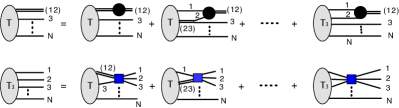
Figure 1: Diagrammatic representation of Eq.(13) and Eq.(14), pair-wise and three-body interactions are represented by black solid circle and blue solid square.

II.2 Three-boson dynamical equations

In the case of $N=3$, the dynamical equations are thus given by

$$T(\mathbf{k}_{3})=\frac{\eta}{L^{3}}\sum_{\mathbf{p}_{2}}\frac{T(\mathbf{k}_{3})+2T(\mathbf{p}_{2})+T_{3}}{E-\frac{(\mathbf{k}_{1}+\mathbf{k}_{2}-\mathbf{p}_{2})^{2}+\mathbf{p}_{2}^{2}+\mathbf{k}^{2}_{3}}{2m}},$$ (15)

and

$$T_{3}=\frac{\eta_{3}}{L^{6}}\sum_{\mathbf{p}_{2},\mathbf{p}_{3}}\frac{3T(\mathbf{p}_{2})+T_{3}}{E-\frac{\mathbf{p}_{2}^{2}+\mathbf{p}_{3}^{2}+(\mathbf{P}-\mathbf{p}_{2}-\mathbf{p}_{3})^{2}}{2m}}.$$ (16)

Eliminating $T_{3}$ amplitude, we find

$$T(\mathbf{k}_{3})=\frac{\eta}{L^{3}}\sum_{\mathbf{p}_{2}}\frac{1}{E-\frac{\mathbf{p}_{2}^{2}+(\mathbf{k}_{1}+\mathbf{k}_{2}-\mathbf{p}_{2})^{2}+\mathbf{k}^{2}_{3}}{2m}}\Bigg{[}T(\mathbf{k}_{3})+2T(\mathbf{p}_{2})$$

$$\quad\quad\quad+\frac{\frac{\eta_{3}}{L^{6}}\sum_{\mathbf{q}_{2},\mathbf{q}_{3}}\frac{3T(\mathbf{q}_{2})}{E-\frac{\mathbf{q}_{2}^{2}+\mathbf{q}_{3}^{2}+(\mathbf{P}-\mathbf{q}_{2}-\mathbf{q}_{3})^{2}}{2m}}}{1-\frac{\eta_{3}}{L^{6}}\sum_{\mathbf{q}_{2},\mathbf{q}_{3}}\frac{1}{E-\frac{\mathbf{q}_{2}^{2}+\mathbf{q}_{3}^{2}+(\mathbf{P}-\mathbf{q}_{2}-\mathbf{q}_{3})^{2}}{2m}}}\Bigg{]}.$$ (17)

III Threshold Expansion

In this section, we illustrate that the threshold expansion formula may be derived from Eqs.(13) and (14) by iterations. Near the ground state energy threshold, all $N$ particles are nearly at rest for weak interactions. Hence the dominant contribution comes from the zero momenta mode of amplitudes: $\{\mathbf{k}\}=\{\mathbf{0}\}$. Thus, we find

$$\left[1-\frac{\eta}{L^{3}}\sum_{\mathbf{p}_{2}}\frac{1}{E-\frac{\mathbf{p}_{2}^{2}}{m}}\right]T(\overline{\{\mathbf{0}\}}_{(12)})$$

$$=\frac{\eta}{L^{3}}\sum_{\mathbf{p}_{2}}\frac{\sum_{i<j}^{(ij)\neq(12)}T(\overline{\{\mathbf{p}\}}_{(ij)})+\sum_{i<j<k}T_{3}(\overline{\{\mathbf{p}\}}_{(ijk)})}{E-\frac{\mathbf{p}_{2}^{2}}{m}},$$

$$\quad\mathbf{p}_{1}=-\mathbf{p}_{2},\ \ \mathbf{p}_{l}=\mathbf{0},\ \ l=3,\cdots,N,$$ (18)

and

$$T_{3}(\overline{\{\mathbf{0}\}}_{(123)})$$

$$=\frac{\eta_{3}}{L^{6}}\sum_{\mathbf{p}_{2},\mathbf{p}_{3}}\frac{\sum_{i<j}T(\overline{\{\mathbf{p}\}}_{(ij)})+\sum_{i<j<k}T_{3}(\overline{\{\mathbf{p}\}}_{(ijk)})}{E-\frac{\mathbf{p}_{2}^{2}+\mathbf{p}_{3}^{2}+(\mathbf{p}_{2}+\mathbf{p}_{3})^{2}}{2m}},$$

$$\quad\mathbf{p}_{1}=-\mathbf{p}_{2}-\mathbf{p}_{3},\ \ \mathbf{p}_{l}=\mathbf{0},\ \ l=4,\cdots,N.$$ (19)

III.1 Perturbation expansion by iteration of $N$-body dynamical equations

As we can see from above equations, the leading order contributions of $T$ and $T_{3}$ start at the order of $\frac{\eta}{L^{3}}$ and $\frac{\eta_{3}}{L^{6}}$ respectively. In present work, the aim is to just simply illustrate how the threshold expansion formula are derived from Eqs.(13) and (14). For this purpose, we will only compute up to $\eta^{3}/L^{5}$ order in threshold expansion formula by iterating Eqs.(13) and (14) only once. The contributions from three-body force are only kept at the lowest order effect, and also splitting up zero momenta mode and non-zero momenta mode contributions in Eq.(18), so we obtain

$$\left[1-\frac{\eta}{L^{3}}\sum_{\mathbf{p}_{2}\neq\mathbf{0}}\frac{1}{E-\frac{\mathbf{p}_{2}^{2}}{m}}-\frac{\eta}{L^{3}}\frac{\frac{N(N-1)}{2}}{E}\right]T(\overline{\{\mathbf{0}\}}_{(12)})$$

$$=\frac{\eta}{L^{3}}\sum_{\mathbf{p}_{2}\neq\mathbf{0}}\frac{\sum_{i<j}^{(ij)\neq(12)}T(\overline{\{\mathbf{p}\}}_{(ij)})}{E-\frac{\mathbf{p}_{2}^{2}}{m}}$$

$$+\frac{\eta}{L^{3}}\frac{\frac{N(N-1)(N-2)}{6}}{E}T_{3}(\overline{\{\mathbf{0}\}}_{(123)})+\mathcal{O}(\frac{\eta^{2}\eta_{3}}{L^{12}}),$$

$$\quad\mathbf{p}_{1}=-\mathbf{p}_{2},\ \ \ \ \mathbf{p}_{l}=\mathbf{0},\ \ l=3,\cdots,N,$$ (20)

and

$$T_{3}(\overline{\{\mathbf{0}\}}_{(123)})=\frac{\eta_{3}}{L^{6}}\frac{\frac{N(N-1)}{2}}{E}T(\overline{\{\mathbf{0}\}}_{(12)})+\mathcal{O}(\frac{\eta\eta_{3}}{L^{9}}).$$ (21)

Eliminating $T_{3}(\overline{\{\mathbf{0}\}}_{(123)})$ term in Eq.(20), we find

$$\left[1-\frac{\eta}{L^{3}}\sum_{\mathbf{p}_{2}\neq\mathbf{0}}\frac{1}{E-\frac{\mathbf{p}_{2}^{2}}{m}}-\frac{\eta}{L^{3}}\frac{\frac{N(N-1)}{2}}{E}\right]T(\overline{\{\mathbf{0}\}}_{(12)})$$

$$=\frac{\eta\eta_{3}}{L^{9}}\frac{\frac{N^{2}(N-1)^{2}(N-2)}{12}}{E^{2}}T(\overline{\{\mathbf{0}\}}_{(12)})$$

$$+\frac{\eta}{L^{3}}\sum_{\mathbf{p}_{2}\neq\mathbf{0}}\frac{\sum_{i<j}^{(ij)\neq(12)}T(\overline{\{\mathbf{p}\}}_{(ij)})}{E-\frac{\mathbf{p}_{2}^{2}}{m}}+\mathcal{O}(\frac{\eta^{2}\eta_{3}}{L^{12}}),$$

$$\quad\mathbf{p}_{1}=-\mathbf{p}_{2},\ \ \ \ \mathbf{p}_{l}=\mathbf{0},\ \ l=3,\cdots,N.$$ (22)

Now, dominant zero momenta mode and sub-leading non-zero momenta mode are well separated in Eq.(22). The terms that are given by non-zero momenta mode of $T$ amplitudes in Eq.(22) can be eliminated and thus are related to zero momenta mode amplitudes by iterating Eq.(13) once.

Non-zero momenta mode of set $\overline{\{\mathbf{p}\}}_{(ij)}$ in $T(\overline{\{\mathbf{p}\}}_{(ij)})$ can be split into two groups: (1) $\overline{\{\mathbf{p}\}}_{(1j)}=\{\mathbf{0},\cdots,\mathbf{p}_{2},\cdots,\mathbf{0}\}$ with only a single non-zero momentum dependence at j-th position, $\mathbf{p}_{j}=\mathbf{p}_{2}$ and $j>2$; (2) $\overline{\{\mathbf{p}\}}_{(ij)}=\{\mathbf{0},\cdots,-\mathbf{p}_{2},\cdots,\mathbf{p}_{2},\cdots,\mathbf{0}\}$ with two non-zero momenta dependence at i-th and j-th positions, $\mathbf{p}_{i}=-\mathbf{p}_{2}$ and $\mathbf{p}_{j}=\mathbf{p}_{2}$, where $(i<j)=3,\cdots,N$.

(1) For amplitudes in group one with only a single non-zero momentum dependence, using Eq.(13) again, we find that each non-zero mode $T(\overline{\{\mathbf{p}\}}_{(1j)})$ is related to two amplitudes that doesn’t depend on $\mathbf{p}_{2}$,

$$T(\overline{\{\mathbf{p}\}}_{(1j)})$$

$$=\frac{\eta}{L^{3}}\left[\sum_{\mathbf{q}_{2}}\frac{T(\overline{\{\mathbf{q}\}}_{(1j)})}{E-\frac{\mathbf{q}_{1}^{2}+\mathbf{q}_{2}^{2}+\mathbf{p}^{2}_{2}}{2m}}+\sum_{\mathbf{q}_{1}}\frac{T(\overline{\{\mathbf{q}\}}_{(2j)})}{E-\frac{\mathbf{q}_{1}^{2}+\mathbf{q}_{2}^{2}+\mathbf{p}^{2}_{2}}{2m}}\right]+\cdots$$

$$=\frac{\eta}{L^{3}}\sum_{\mathbf{q}_{2}}\frac{2T(\overline{\{\mathbf{q}\}}_{(1j)})}{E-\frac{(\mathbf{p}_{2}+\mathbf{q}_{2})^{2}+\mathbf{q}_{2}^{2}+\mathbf{p}^{2}_{2}}{2m}}+\cdots,$$ (23)

where $\overline{\{\mathbf{q}\}}_{(1j)}=\{\mathbf{0},\cdots,\mathbf{q}_{2},\cdots,\mathbf{0}\}$ and $\overline{\{\mathbf{q}\}}_{(2j)}=\{\mathbf{0},\cdots,\mathbf{q}_{1},\cdots,\mathbf{0}\}$ with $\mathbf{q}_{2}$ and $\mathbf{q}_{1}$ siting at j-th position. Splitting sum of $\mathbf{q}_{2}$ to zero momenta mode and non-zero momenta mode again in Eq.(23), the dominant contribution for $T(\overline{\{\mathbf{p}\}}_{(1j)})$ comes from zero momenta mode, sub-leading contribution from non-zero momenta mode may be eliminated by iteration again. Keeping only dominant zero momenta mode contribution, we hence find

$$T(\overline{\{\mathbf{p}\}}_{(1j)})=\frac{\eta}{L^{3}}\frac{1}{E-\frac{\mathbf{p}_{2}^{2}}{m}}2T(\overline{\{\mathbf{0}\}}_{(12)})+\mathcal{O}(\frac{\eta\eta_{3}}{L^{6}}).$$ (24)

There are $(N-2)$ terms of $T(\overline{\{\mathbf{p}\}}_{(1j)})$ in group one, and another $(N-2)$ equivalent terms for $T(\overline{\{\mathbf{p}\}}_{(2j)})$ amplitudes. Therefore, the total dominant contribution from group one is $\frac{\eta}{L^{3}}\frac{4(N-2)}{E-\frac{\mathbf{p}_{2}^{2}}{m}}T(\overline{\{\mathbf{0}\}}_{(12)})$.

(2) For amplitudes in group two with two non-zero momentum dependence, each $T(\overline{\{\mathbf{p}\}}_{(ij)})$ is related to only one amplitude that does not depend on $\mathbf{p}_{i}=-\mathbf{p}_{2}$ and $\mathbf{p}_{j}=\mathbf{p}_{2}$,

$$T(\overline{\{\mathbf{p}\}}_{(ij)})=\frac{\eta}{L^{3}}\sum_{\mathbf{q}_{2}}\frac{T(\overline{\{\mathbf{q}\}}_{(ij)})}{E-\frac{\mathbf{q}_{2}^{2}+\mathbf{p}^{2}_{2}}{m}}+\cdots,$$ (25)

where $\overline{\{\mathbf{q}\}}_{(ij)}=\{\mathbf{0},\cdots,-\mathbf{q}_{2},\cdots,\mathbf{q}_{2},\cdots,\mathbf{0}\}$ with $-\mathbf{q}_{2}$ and $\mathbf{q}_{2}$ siting at i-th and j-th positions respectively. Hence, the dominant zero momenta mode contribution from $T(\overline{\{\mathbf{p}\}}_{(ij)})$ term is

$$T(\overline{\{\mathbf{p}\}}_{(ij)})=\frac{\eta}{L^{3}}\frac{1}{E-\frac{\mathbf{p}_{2}^{2}}{m}}T(\overline{\{\mathbf{0}\}}_{(12)})+\mathcal{O}(\frac{\eta\eta_{3}}{L^{6}}).$$ (26)

There are $\frac{(N-2)(N-3)}{2}$ such terms, the total number of dominant contribution from group two is thus $\frac{\eta}{L^{3}}\frac{\frac{(N-2)(N-3)}{2}}{E-\frac{\mathbf{p}_{2}^{2}}{m}}T(\overline{\{\mathbf{0}\}}_{(12)})$.

III.1.1 Zero momenta mode $N$-boson dynamical equation

Combining all non-zero momenta mode terms in Eq.(22) from both group one and group two, we obtain,

$$\frac{\eta}{L^{3}}\sum_{\mathbf{p}_{2}\neq\mathbf{0}}\frac{\sum_{i<j}^{(ij)\neq(12)}T(\overline{\{\mathbf{p}\}}_{(ij)})}{E-\frac{\mathbf{p}_{2}^{2}}{m}}$$

$$=\frac{\eta^{2}}{L^{6}}\sum_{\mathbf{p}_{2}\neq\mathbf{0}}\frac{4(N-2)+\frac{(N-2)(N-3)}{2}}{\left(E-\frac{\mathbf{p}_{2}^{2}}{m}\right)^{2}}+\mathcal{O}(\frac{\eta^{2}\eta_{3}}{L^{12}}).$$ (27)

Plugging them back into Eq.(20), we thus find

$$\left[1-\frac{\eta}{L^{3}}\sum_{\mathbf{p}_{2}\neq\mathbf{0}}\frac{1}{E-\frac{\mathbf{p}_{2}^{2}}{m}}-\frac{\eta}{L^{3}}\frac{\frac{N(N-1)}{2}}{E}\right]T(\overline{\{\mathbf{0}\}}_{(12)})$$

$$=\frac{\eta\eta_{3}}{L^{9}}\frac{\frac{N^{2}(N-1)^{2}(N-2)}{12}}{E^{2}}T(\overline{\{\mathbf{0}\}}_{(12)})$$

$$+\frac{\eta^{2}}{L^{6}}\sum_{\mathbf{p}_{2}\neq\mathbf{0}}\frac{\frac{(N-2)(N+5)}{2}}{\left(E-\frac{\mathbf{p}_{2}^{2}}{m}\right)^{2}}T(\overline{\{\mathbf{0}\}}_{(12)})+\mathcal{O}(\frac{\eta^{2}\eta_{3}}{L^{12}}).$$ (28)

Zero momenta mode amplitude $T(\overline{\{\mathbf{0}\}}_{(12)})$ is thus cancelled out from both sides of equation, and Eq.(28) yields an analytic form that depends on only $E$ and momentum sum.

III.1.2 Three-boson example

Using three-body dynamical equation given in Eq.(17) as a specific example, setting $\mathbf{k}_{1}=\mathbf{k}_{2}=\mathbf{k}_{3}=\mathbf{0}$, and keep only up to $\frac{\eta\eta_{3}}{L^{9}}$ order, we obtain

$$T(\mathbf{0})\simeq\frac{\eta}{L^{3}}\sum_{\mathbf{p}_{2}}\frac{T(\mathbf{0})+2T(\mathbf{p}_{2})}{E-\frac{\mathbf{p}_{2}^{2}}{m}}+\frac{\eta\eta_{3}}{L^{9}}\frac{3T(\mathbf{0})}{E^{2}}.$$ (29)

Splitting up to zero momenta and non-zero momenta mode in Eq.(29), and also use Eq.(17) once to eliminate non-zero momenta mode,

$$T(\mathbf{p}_{2})=\frac{\eta}{L^{3}}\frac{2T(\mathbf{0})}{E-\frac{\mathbf{p}^{2}_{2}}{m}}+\cdots,\ \ \mathbf{p}_{2}\neq\mathbf{0},$$ (30)

hence we finally get

$$1-\frac{\eta}{L^{3}}\sum_{\mathbf{p}_{2}\neq\mathbf{0}}\frac{1}{E-\frac{\mathbf{p}_{2}^{2}}{m}}-\frac{\eta}{L^{3}}\frac{3}{E}$$

$$\simeq\frac{\eta^{2}}{L^{6}}\sum_{\mathbf{p}_{2}\neq\mathbf{0}}\frac{4}{\left(E-\frac{\mathbf{p}_{2}^{2}}{m}\right)^{2}}+\frac{\eta\eta_{3}}{L^{9}}\frac{3}{E^{2}}.$$ (31)

III.2 Near threshold expansion and ground state energy

By assuming that energy shift near threshold is small due to weak interactions: $E\sim 0$, Eq.(28) is thus turned into a polynomial equation by near threshold expansion, keeping up to $\mathcal{O}(E^{3})$, we have

$$\mathcal{O}(E^{4})+\left(\frac{1}{L^{3}}\sum_{\mathbf{p}\neq\mathbf{0}}\frac{1}{\frac{\mathbf{p}^{4}}{m^{2}}}\right)E^{3}$$

$$+\left(\frac{1}{\eta}+\frac{1}{L^{3}}\sum_{\mathbf{p}\neq\mathbf{0}}\frac{1}{\frac{\mathbf{p}^{2}}{m}}-\frac{\eta}{L^{6}}\sum_{\mathbf{p}\neq\mathbf{0}}\frac{\frac{(N+5)(N-2)}{2}}{\frac{\mathbf{p}^{4}}{m^{2}}}\right)E^{2}$$

$$-\frac{1}{L^{3}}\frac{N(N-1)}{2}E=\frac{\eta_{3}}{L^{9}}\frac{N^{2}(N-1)^{2}(N-2)}{12}.$$ (32)

Introducing renormalized two-body coupling constant

$$\frac{1}{\eta}=\frac{1}{\eta_{R}}-\frac{m\Lambda}{\pi L},$$ (33)

where $\Lambda$ is related to the cutoff on momentum sum, and also using relations given in Refs. Beane et al. (2007),

$$\frac{1}{L^{3}}\sum_{\mathbf{p}_{1}\neq\mathbf{0}}\frac{1}{\frac{\mathbf{p}_{1}^{2}}{m}}-\frac{m\Lambda}{\pi L}=\frac{m\mathcal{I}}{(2\pi)^{2}L},\ \ \ \ \mathcal{I}=\sum_{\mathbf{n}\neq\mathbf{0}}^{|\mathbf{n}|\leqslant\Lambda}\frac{1}{\mathbf{n}^{2}}-4\pi\Lambda,$$

$$\frac{1}{L^{3}}\sum_{\mathbf{p}_{1}\neq\mathbf{0}}\frac{1}{\frac{\mathbf{p}_{1}^{4}}{m^{2}}}=\frac{m^{2}L\mathcal{J}}{(2\pi)^{4}},\ \ \ \ \mathcal{J}=\sum_{\mathbf{n}\neq\mathbf{0}}\frac{1}{\mathbf{n}^{4}},$$ (34)

we can rewrite Eq.(32) to

$$\frac{L\mathcal{J}}{(2\pi)^{4}}(mE)^{3}$$

$$+\left(\frac{1}{m\eta_{R}}+\frac{\mathcal{I}}{(2\pi)^{2}L}-\frac{(N+5)(N-2)}{2}\frac{m\eta_{R}\mathcal{J}}{(2\pi)^{4}L^{2}}\right)(mE)^{2}$$

$$-\frac{1}{L^{3}}\frac{N(N-1)}{2}(mE)\simeq\frac{m\eta_{3}}{L^{9}}\frac{N^{2}(N-1)^{2}(N-2)}{12}.$$ (35)

The cubic equation, Eq.(35), can be easily solved by perturbation theory

$$mE=\frac{N(N-1)}{2}\frac{4\pi a_{0}}{L^{3}}\left[1+\sum_{n=1}^{3}\left(\frac{a_{0}}{\pi L}\right)^{n}c_{n}\right],$$ (36)

where $a_{0}$ is two-body scattering length and is related to coupling constant of pair-wise contact interaction by

$$m\eta_{R}=4\pi a_{0}.$$ (37)

The solution of cubic equation, Eq.(35) is thus given by

$$E =\frac{N(N-1)}{2}\frac{4\pi a_{0}}{mL^{3}}\bigg{[}1-\left(\frac{a_{0}}{\pi L}\right)\mathcal{I}$$

$$+\left(\frac{a_{0}}{\pi L}\right)^{2}\left(\mathcal{I}^{2}+(2N-5)\mathcal{J}\right)+\mathcal{O}(\frac{a^{3}_{0}}{L^{3}})\bigg{]}$$

$$+\frac{N(N-1)(N-2)}{6}\frac{\eta_{3}}{L^{6}},$$ (38)

which is consistent with well-known results in Refs. Huang and Yang (1957); Lee et al. (1957); Beane et al. (2007); Detmold and Savage (2008).

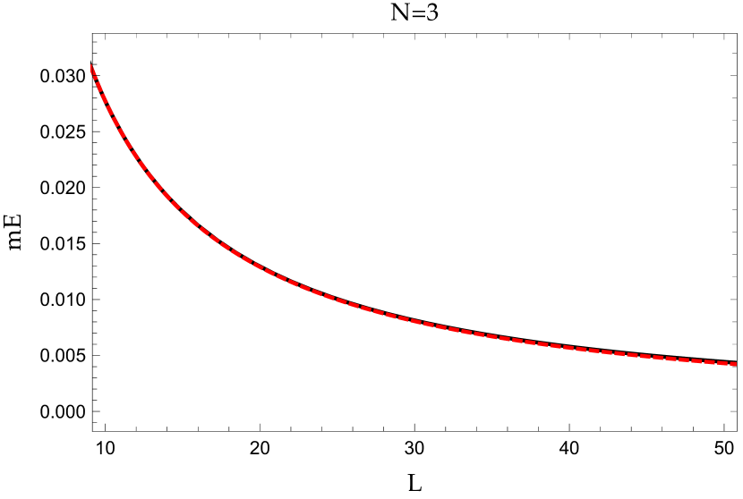
(a) Three-boson energy spectrum in 1D.

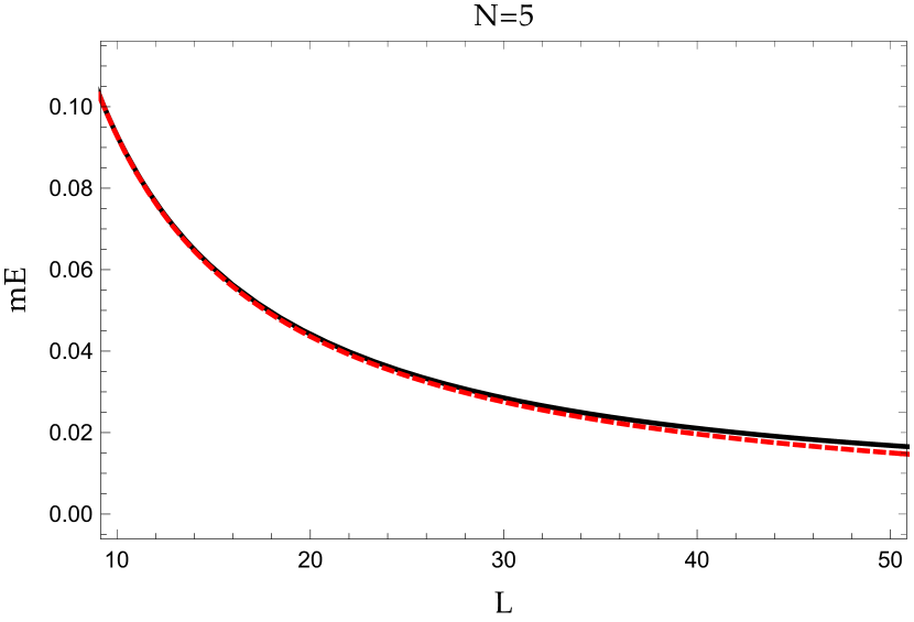
(b) Five-boson energy spectrum in 1D.

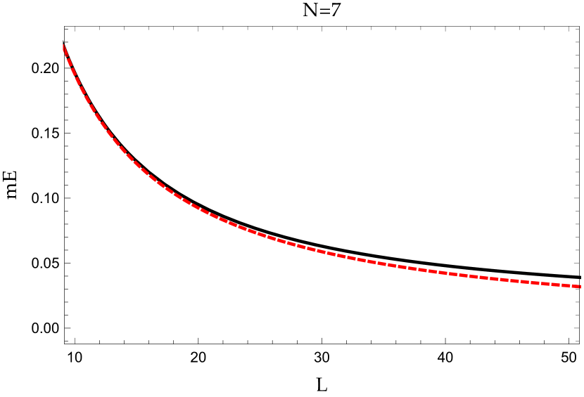
(c) Seven-boson energy spectrum in 1D.

Figure 2: Plot of $mE$ as the function of $L$: red dashed curves are exact solutions given by Eq.(39), and black solid curves are approximate solution given by threshold expansion in Eq.(42), $m\eta=0.1$.

III.3 Threshold expansion formula in 1D and comparison to exact solutions

The iteration of coupled finite volume $N$-body dynamical equation approach and results presented in section III.1 and III.2 can be applied to $N$-boson interaction in 1D with little changes. $N$ identical bosons interacting with pair-wise contact potentials in 1D is in fact exactly solvable, see Refs. Yang (1967); Lieb and Liniger (1963); Guo (2017). The exact analytic solutions are given by $E=\frac{1}{2m}\sum_{i=1}^{N}p_{i}^{2}$, where $p_{i}$’s satisfies coupled equations

$$\frac{p_{i}L}{2}=\sum_{j=1(j\neq i)}^{N}\cot^{-1}\left(\frac{p_{i}-p_{j}}{m\eta}\right),\ \ \sum_{i=1}^{N}p_{i}=0.$$ (39)

Keeping only pair-wise contact interaction and expanding up to $\mathcal{O}(E^{3})$, the threshold expansion equation in 1D can be obtained by replacing 3D momentum sum $\frac{1}{L^{3}}\sum_{\mathbf{p}}$ in Eq.(32) by 1D counterpart $\frac{1}{L}\sum_{p}$, hence, we obtain

$$\frac{1}{L}\frac{N(N-1)}{2}\simeq\left(\frac{1}{L}\sum_{p\neq 0}\frac{1}{p^{4}}\right)(mE)^{2}$$

$$+\left(\frac{1}{m\eta}+\frac{1}{L}\sum_{p\neq 0}\frac{1}{p^{2}}-\frac{\eta}{L^{2}}\sum_{p\neq 0}\frac{\frac{(N+5)(N-2)}{2}}{p^{4}}\right)(mE).$$ (40)

The infinite momentum sum in 1D can be carried out rather easily,

$$\sum_{p\neq 0}\frac{1}{p^{2}}=\frac{L^{2}}{12},\ \ \ \ \sum_{p\neq 0}\frac{1}{p^{4}}=\frac{L^{4}}{720},$$ (41)

the solution of Eq.(40) is thus given by

$$mE=\frac{\sqrt{b^{2}+4c}-b}{2},$$ (42)

where

$$b =\frac{720}{L^{3}}\left(\frac{1}{m\eta}+\frac{L}{12}-\frac{(N+5)(N-2)}{2}\frac{m\eta L^{2}}{720}\right),$$

$$c =\frac{N(N-1)}{2}\frac{720}{L^{4}}.$$ (43)

The comparison of $mE$ as the function of $L$ between exact solutions given by Eq.(39) and approximate solution by threshold expansion in Eq.(42) is illustrated in Fig. 2.

IV Summary

As a sanity check and a test on the formalism of finite volume $N$-body system developed in Guo et al. (2018); Guo (2019); Guo and Döring (2020), we illustrate how the well-known threshold expansion formula of $N$-identical-boson system may be derived by iterations of Faddeev-type coupled dynamical equations. The ground state energy of $N$-boson system near threshold is dominated by zero momenta mode of $N$-body amplitudes, non-zero momenta mode amplitudes are associated with sub-leading order contributions and are related to leading order zero momenta mode through Faddeev-type coupled dynamical equations. Eliminating non-zero momenta modes by iterations ultimately yields an analytic expression that depends on only system energy and free momentum sum, thus it can be turned into a polynomial equation by treating energy shift near threshold as a small parameter. With only a single iteration, we are able to compute threshold expansion formula up to $\mathcal{O}(\eta^{3}/L^{5})$ for pair-wise interaction and $\mathcal{O}(\eta_{3}/L^{6})$ for three-body interaction.