Lyman-$\alpha$ Polarization Intensity Mapping

Abstract

We present a formalism that incorporates hydrogen Lyman-alpha (Ly$\alpha$) polarization arising from the scattering of radiation in galaxy halos into the intensity mapping approach. Using the halo model, and Ly$\alpha$ emission profiles based on simulations and observations, we calcualte auto and cross power spectra at redshifts $3\leq z\leq 13$ for the Ly$\alpha$ total intensity, $I$, polarized intensity, $\pazocal{P}$, degree of polarization, $\Pi=\pazocal{P}/I$, and two new quantities, the astrophysical $E$ and $B$ modes of Ly$\alpha$ polarization. The one-halo terms of the $\Pi$ power spectra show a turnover that signals the average extent of the polarization signal, and thus the extent of the scattering medium. The position of this feature depends on redshift, as well as on the specific emission profile shape and extent, in our formalism. Therefore, the comparison of various Ly$\alpha$ polarization quantities and redshifts can break degeneracies between competing effects, and it can reveal the true shape of the emission profiles, which, in turn, are associated to the physical properties of the cool gas in galaxy halos. Furthermore, measurements of Ly$\alpha$ $E$ and $B$ modes may be used as probes of galaxy evolution, because they are related to the average degree of anisotropy in the emission and in the halo gas distribution across redshifts. The detection of the polarization signal at $z\sim 3-5$ requires improvements in the sensitivity of current ground-based experiments by a factor of $\sim 10$, and of $\sim 100$ for space-based instruments targeting the redshifts $z\sim 9-10$, the exact values depending on the specific redshift and experiment. Interloper contamination in polarization is expected to be small, because the interlopers need to also be polarized. Overall, Ly$\alpha$ polarization boosts the amount of physical information retrievable on galaxies and their surroundings, most of it not achievable with total emission alone.

1 Introduction

Intensity mapping (IM) is a novel method to study the formation and evolution of galaxies, by statistically analyzing the collective emission present in large areas of the sky, and at different epochs, regardless of the number of bright (individually detectable) sources in them (Madau et al., 1997; Suginohara et al., 1999; Visbal & Loeb, 2010, see the recent review by Kovetz et al. 2017). The IM methodology takes into account the emission from the entire galaxy population, and thus, contrary to more traditional galaxy studies, it is not limited to the sources above observational detection thresholds.

IM considers a broad range of frequencies and emission lines, such as those of [Cii] at 158 $\mu$m (e.g., Gong et al., 2012; Silva et al., 2015; Yue et al., 2015), the CO molecule (e.g., Righi et al., 2008; Gong et al., 2011; Lidz et al., 2011; Pullen et al., 2013; Chung et al., 2019), the hydrogen 21cm spin-flip transition (e.g., Scott & Rees, 1990; Madau et al., 1997; Chang et al., 2008, 2010; Switzer et al., 2013), or X-rays, as recently proposed by Caputo et al. (2019).

In addition to the aforementioned frequencies, the hydrogen Lyman-alpha (Ly$\alpha$) radiation is one of the main targets of IM. Ly$\alpha$ emission is especially useful for studies of cosmic reionization at $z\gtrsim 5$ (e.g., Silva et al., 2013; Pullen et al., 2014), but also for studies up to the pre-reionization epoch at $z\sim 20-30$ (Loeb & Rybicki, 1999), and down to the peak of cosmic star formation at $z\sim 2-3$ (e.g., Hogan & Weymann, 1987; Gould & Weinberg, 1996; Croft et al., 2018). In these cases, Ly$\alpha$ is mostly produced by young (blue) stars, and it is the brightest emission line from star formation (Partridge & Peebles, 1967).

A particular characteristic of Ly$\alpha$ radiation compared to other emission lines, is its resonant nature. Because Ly$\alpha$ is the only radiative channel allowed by quantum mechanics between the hydrogen ground and first excited atomic states, the absorption of a Ly$\alpha$ photon by a hydrogen atom (Hi) typically results in the immediate emission of another Ly$\alpha$ photon. This is the well-known Ly$\alpha$ scattering process, which enables the Ly$\alpha$ photons to transfer (diffuse) through a neutral hydrogen medium, until the photons escape the medium or they become destroyed by dust (see Dijkstra, 2014, for a review). Scattering, together with other potential mechanisms (see Mas-Ribas et al., 2017a, for a discussion of the various processes), contributes to the diffuse and extended Ly$\alpha$ emission currently detectable with instruments such as MUSE (Bacon et al., 2014) or KCWI (Morrissey et al., 2018), down to surface brightness levels of $\sim 10^{-19}\,{\rm erg\,s^{-1}\,cm^{-2}\,arcsec^{-2}}$, and out to several tens of physical kpc from the center of most individual $2\lesssim z\lesssim 7$ star-forming galaxies and quasars, constituting the so-called Ly$\alpha$ halos (e.g., Borisova et al., 2016; Wisotzki et al., 2016; Leclercq et al., 2017; Wisotzki et al., 2018; Arrigoni Battaia et al., 2019; Farina et al., 2019). The IM approach will enable studying this faint emission far from the sources for a large number of objects statistically, as well as the Ly$\alpha$ emission arising directly from the distant intergalactic medium, especially at redshifts $z\gtrsim 3-5$, where the fraction of cosmic neutral hydrogen gas is significant (e.g., Gould & Weinberg, 1996; Loeb & Rybicki, 1999; Laursen et al., 2011; Silva et al., 2013; Pullen et al., 2014; Davies et al., 2016; Kakiichi et al., 2016; Visbal & McQuinn, 2018).

In this paper, we focus on the polarization of Ly$\alpha$ radiation around galaxies, which is another effect arising from the scattering of Ly$\alpha$ photons, and that has not been previously considered in the intensity mapping formalism. Because in the scattering event the Ly$\alpha$ photons become polarized (e.g., Chandrasekhar, 1960), and because scattering contributes to the extended Ly$\alpha$ emission around sources, a net polarization fraction can appear in the diffuse Ly$\alpha$ emission in galaxy halos. Indeed, Rybicki & Loeb (1999) first noted that high degrees of Ly$\alpha$ polarization, up to $\sim 40-60\,\%$, could occur around pre-reionization sources due to Ly$\alpha$ radiation scattered by the neutral intergalactic gas. Later, Dijkstra & Loeb (2008) performed Ly$\alpha$ radiative transfer simulations in idealized spherically-symmetric expanding Hi shells, resembling the environment around high-redshift galaxies, and showed that this polarization signal can also be found in the halo of $z\sim 5-6$ galaxies (see also Dijkstra & Kramer, 2012). These calculations indicated that the degree of polarization increases with impact parameter, from a few per cent at the center to a few tens of per cent at large impact parameters, and that the angle of polarization forms concentric rings projected on the sky around the radiation source. Observations confirming these theoretically-predicted trends were presented by Hayes et al. (2011), and supported more recently by Beck et al. (2016) and Herenz et al. (2020), for a bright and extended Ly$\alpha$ nebula at $z\approx 3$, LAB1; Steidel et al. (2000). Unlike Ly$\alpha$ halos around individual galaxies, Ly$\alpha$ nebulae or blobs can be powered by bright and/or multiple sources, such as quasars or bright galaxies, and they typically extend to distances on the order of $\gtrsim 100$ physical kpc, larger than typical Ly$\alpha$ halos. Hayes et al. (2011) found a polarization fraction value increasing from a few per cent around the center of the brightest LAB1 region, up to $\sim 18\,\%$ at $\sim 50$ pkpc, beyond which the signal-to-noise ratio did not enable precise measurements (see their Figure 3). The measured polarization pattern broadly agreed with the circular (tangential) directions predicted by the numerical models, but there are cases where the differences are significant (see Figure S3 in Hayes et al., 2011). These differences are not surprising, because the actual environment around LAB1 is not spherically symmetric, as was the case in the numerical work of Dijkstra & Loeb (2008), and because several sources could contribute to the Ly$\alpha$ emission, as demonstrated by the observations and simulations of LAB1 by Geach et al. 2016 (although see Trebitsch et al., 2016, where their numerical simulations favor a gravitational cooling scenario driving the observations). Prescott et al. (2011) performed observations of another Ly$\alpha$ blob at $z\sim 2.6$, LABd05; Dey et al. (2005), but their low spatial resolution enabled them to only set an upper limit of $\sim 2.5\,\%$ for the polarization fraction in a single aperture with radius $\sim 33$ kpc. More recently, Humphrey et al. (2013) and You et al. (2017) have also reported Ly$\alpha$ polarization observations in Ly$\alpha$ nebulae at $z\approx 2.3$ and $z\approx 3$, respectively. Their results are in broad agreement with those found by Hayes et al. (2011).

Given the ubiquitous extended and diffuse Ly$\alpha$ emission around high-redshift sources that overall covers large portions of the sky (see Figure 1 in Wisotzki et al., 2018), it is plausible to expect also a global Ly$\alpha$ polarization signal. The exact value of the degree of polarization depends strongly on the physical properties of the scattering medium (i.e., its bulk and turbulent velocity, as well as its Hi density). The Ly$\alpha$ polarization pattern (i.e., the angle of polarization) around the sources depends strongly on the isotropy and homogeneity of the emission and gas distribution (Lee & Ahn, 1998; Ahn et al., 2002; Chang et al., 2016; Eide et al., 2018). These dependences make the polarization signal very sensitive to the specific conditions of the medium, and, as we will show, this boosts the amount of information on galaxies and their environment retrievable from polarization, compared to that from emission alone. The goal of this work is to provide a first theoretical benchmark to assess the utility of such a polarized emission, and to investigate whether the expected signal is within reach of current and future intensity mapping experiments.

In § 2 below, we derive the mathematical formalism for characterizing the global polarized Ly$\alpha$ signal. The physical origin and modeling of the Ly$\alpha$ emission around sources is detailed in § 3. The results and estimates for the detectability are presented in § 4 and § 5, respectively. We discuss the case of Ly$\alpha$ B modes in § 6, future work in § 7, and conclude in § 8.

We assume a flat ($\Omega_{\rm k}=0$) $\Lambda$CDM cosmology with the parameter values from Planck Collaboration et al. (2016), and use comoving units throughout unless stated otherwise.

2 A Halo Model Formalism for Ly$\alpha$ Polarization

This section describes a simple formalism for parameterizing the Ly$\alpha$ polarization signal. We use the halo model to assess the spatial distribution of Ly$\alpha$ in § 2.1, and derive the formalism of $E$ and $B$ modes for the case of Ly$\alpha$ polarization in § 2.2. We consider the case of cross-correlations between polarization quantities in § 2.3.

We characterize the polarization signal by considering the four Stokes parameters $I,Q,U,V$. The quantity $I$ is the total intensity of radiation, and the parameters $Q$ and $U$ relate to the polarized radiation along the coordinate axes, and along the directions at $\pi/4$ from them, respectively. This definition implies that the values of $Q$ and $U$ depend on the choice of the coordinate system that defines them, while $I$ is simply a scalar quantity invariant under a change of coordinates (we address this coordinate system dependence in § 2.2). We ignore the parameter describing circular polarization, $V$, because the scattering of Ly$\alpha$ radiation yields linear polarization alone when the incoming radiation is non-circularly polarized, which we assume to be the case here (Chandrasekhar, 1960). Derived quantities also useful for our work are the polarized intensity, $\pazocal{P}=\sqrt{Q^{2}+U^{2}}$, and the degree of polarization (or polarization fraction), $\Pi=\pazocal{P}/I$. For completeness, we define the polarization angle to be $2\gamma=\tan^{-1}(U/Q)$.

To parameterize the spatial distribution of radiation, we adopt the halo model formalism (Peacock & Smith, 2000; Seljak, 2000; Scoccimarro et al., 2001; Cooray & Sheth, 2002). The halo model assumes that all the matter in the universe is contained in spherical halos, and that these halos do not overlap with each other. The signal from the halos is characterized by the one- and two-halo terms, which describe the contribution to the quantity of interest from regions within the same or different halos, respectively. For our work, this description implies that the total power spectra of any quantity can be simply calculated as the sum of the power spectra from the two terms, $P=P^{\rm 1h}+P^{\rm 2h}$, as detailed in the following section.

Below, we derive the two-dimensional (projected) halo-model formalism for the Ly$\alpha$ polarization signal. In practice, the intensity of Ly$\alpha$ radiation, $I$, could be modeled assuming spherical symmetry around the source, which allows one to compute three-dimensional quantities, such as the 3D power spectrum and correlation function. However, the other parameters characterizing the polarization signal are better defined as projected onto the plane of the sky, with a dependence on the impact parameter distance from the center of the emission source (instead of radial distance), and integrated along the line of sight within the source halo.

We assume the validity of the flat-sky approximation throughout, implying that our expressions are consistent with the full curved-sky calculation at multipole values $\ell\gg 1$.

2.1 The 2D Ly$\alpha$ Polarization Power Spectra

We start by expressing the real-space projected signal of $I$ and $\pazocal{P}$ around a halo of mass $M$, and at redshift $z$, as the product of the total amplitude and the profile shape, $I(M)\,u_{I}(r_{\perp}|M,z)$ and $I(M)\,u_{\pazocal{P}}(r_{\perp}|M,z)$, respectively. Here, the amplitude of the intensity only depends on halo mass (see § 3.2), and $\int{\rm d}r_{\perp}2\pi r_{\perp}u_{I}(r_{\perp}|M,z)=1$, where $r_{\perp}$ is the comoving impact parameter from the center of the halo, and $u_{I}$ is the intensity profile shape. Because the polarization degree, $\Pi$, is not directly an additive quantity (one needs to count the intervening photons instead), we do not normalize the profile in this case and simply express the entire signal as $u_{\Pi}(r_{\perp}|M,z)$. With these definitions, we can then write $u_{\pazocal{P}}(r_{\perp}|M,z)=u_{I}(r_{\perp}|M,z)\,u_{\Pi}(r_{\perp}|M,z)$, and equivalently for the amplitude of the polarized intensity, $\pazocal{P}(M)=I(M)\int{\rm d}r_{\perp}2\pi r_{\perp}u_{\pazocal{P}}(r_{\perp}|M,z)$.

The projected Fourier transforms of these real-space profiles are

$$\tilde{u}_{\{I,\pazocal{P},\Pi\}}(\ell|M,z)=\int_{0}^{\infty}{{\rm d}\theta}\,2\pi\theta\,J_{0}(l\theta)\,u_{\{I,\pazocal{P},\Pi\}}\left(\theta=\cfrac{r_{\perp}}{D_{\rm A}(z)}|M,z\right)~{},$$ (1)

where $\theta$ is the angular distance from the center of the halo, resulting from dividing $r_{\perp}$ by the comoving angular diameter distance, $D_{\rm A}(z)$, and the term $J_{0}(l\theta)$ is the Bessel function of the first kind and zeroth order.

Finally, the one- and two-halo terms of the projected power spectra for $I$, $\pazocal{P}$ and $\Pi$ are computed as (see appendix A in Hill & Pajer, 2013)

$$C_{\ell,\,\{I,\pazocal{P},\Pi\}}^{\rm 1h}=\int{\rm d}z\frac{{\rm d}^{2}V}{{\rm d}z\,{\rm d}\Omega}\int{\rm d}M\frac{{\rm d}n}{{\rm d}M}\,w^{2}(M)\,|\tilde{u}_{\{I,\pazocal{P},\Pi\}}(\ell|M,z)|^{2}~{},$$ (2)

and

$$C_{\ell,\,\{I,\pazocal{P},\Pi\}}^{\rm 2h}=\int{\rm d}z\frac{{\rm d}^{2}V}{{\rm d}z\,{\rm d}\Omega}P_{\rm lin}\left(k=\frac{\ell+1/2}{\chi(z)},z\right)\left[\int{\rm d}M\frac{{\rm d}n}{{\rm d}M}\,b_{\{I,\pazocal{P},\Pi\}}\,w(M)\,\tilde{u}_{\{I,\pazocal{P},\Pi\}}(\ell|M,z)\right]^{2}.$$ (3)

The term ${{\rm d}^{2}V}/{{\rm d}z\,{\rm d}\Omega}={c\,\chi^{2}(z)}/{H(z)}$ is the comoving volume element per steradian and redshift, where $H(z)$ is the Hubble parameter, the speed of light is denoted by $c$, and $\chi(z)$ is the comoving radial distance to redshift $z$. In the above expressions, ${{\rm d}n(M,z)}/{{\rm d}M}$ represents the comoving number density of halos, which depends on halo mass and redshift, and

$$w(M)=\left\{\begin{array}[]{ll}I(M)&\mbox{for}\hskip 5.69054pt\tilde{u}_{\{I,\,\pazocal{P}\}}~{};\\[10.0pt] \cfrac{I(M)}{\bar{I}}&\mbox{for}\hskip 5.69054pt\tilde{u}_{\Pi}~{},\end{array}\right.$$ (6)

where $\bar{I}=\int{\rm d}M\frac{{\rm d}n}{{\rm d}M}\,I(M)$. The use of $I(M)/\bar{I}$ for the polarization degree is motivated by the fact that, in practice, the polarization fraction from observations (simulations) in a given pixel (cell) $i$ is obtained by adding the contribution of all halos $j$ as $\Pi_{i}=\sum_{j}\pazocal{P}_{ij}/\sum_{j}I_{ij}$. We equate this expression in our formalism by weighting the halos by their intensity as $\Pi_{i}=\sum_{j}\Pi_{ij}I_{ij}/\sum_{j}I_{ij}$, where we have used that for an individual halo $\pazocal{P}_{ij}=\Pi_{ij}I_{ij}$. Finally, $P_{\rm lin}(k)$ in Eq. 3 denotes the linear 3D matter density power spectrum and

$$b_{\{I,\pazocal{P},\Pi\}}=\left\{\begin{array}[]{ll}\cfrac{\int{\rm d}M\frac{{\rm d}n}{{\rm d}M}\,b(M)\,I(M)}{\bar{I}}&~{}\mbox{for}\hskip 11.38109pt{I,\pazocal{P}}~{};\\[12.0pt] b(M)&~{}\mbox{for}\hskip 11.38109pt{\Pi}~{},\end{array}\right.$$ (9)

where $b(M)$ denotes the bias for a halo of mass $M$. We adopt an intensity-weighted bias for $I$ and $\pazocal{P}$. However, because in our formalism the extent of $\Pi$ is mostly related to the mass of the halo through the virial radius (§ 3.2), we simply use the halo bias in this case. Biases weighted according to other parameters and properties, e.g., star-formation rate, may be also appropriate depending on the characteristics of the analysis.

An additional consideration in the power spectrum calculation is the shot noise, or Poisson noise, that arises from the discrete sampling of a continuous field. In our models we assume that the Ly$\alpha$ emission is nearly a continuous field, owing to the fact that although Ly$\alpha$ photons are sourced by halos, the signal is diffused away from the central source due to scattering. This extended diffuse emission is described by the Ly$\alpha$ profile in our ‘one-halo term’, which strictly speaking, should be regarded as arising from the Poisson shot noise of discrete sources convolved with the Ly$\alpha$ profile (see the discussion in Wolz et al., 2019, for the case of 21cm studies). We have tested that the strictly-defined $I$ and $\pazocal{P}$ shot-noise terms overall match the amplitudes of the respective one-halo terms of the power spectra at large scales.

Our calculations, therefore, do not include an additional term in the power spectra accounting for the shot noise, as this is essentially our one-halo term. We emphasize that the Ly$\alpha$ one-halo term does not explicitly encapsulate the usual non-linear structure of matter. However, since we use a profile directly from observations that do not resolve small-scale structure, some amount of contribution from faint galaxies populating the dark matter halo may have already been captured (e.g., see the impact of clustered sources on the extended profiles in Mas-Ribas et al., 2017a). We leave a more detailed study to future work.

2.2 The $E$ and $B$ Modes of Ly$\alpha$ Polarization

We derive now the so-called $E$ and $B$ modes for the case of Ly$\alpha$ polarization. These two quantities are related to the $Q$ and $U$ Stokes parameters, but they allow us to obtain polarization information in a coordinate-system-independent manner. The $E$ and $B$ formalism was introduced for CMB analysis by Kamionkowski et al. (1997) and Zaldarriaga & Seljak (1997), and is briefly summarized below.

The total and linearly-polarized intensities, as well as the degree of polarization, $I,\pazocal{P}$ and $\Pi$, respectively, are scalar (spin $s=0$) quantities, and, therefore, their values are invariant under rotations of the coordinate system that defines them. The Stokes $Q$ and $U$ parameters, however, depend on the fixed coordinate system, and transform under a rotation of the coordinate axes by an angle $\alpha$ in the plane of the sky as

$$Q^{\prime}= ~{}Q\cos 2\alpha+U\sin 2\alpha~{},$$ (10)

$$U^{\prime}= -Q\sin 2\alpha+U\cos 2\alpha~{}.$$

Equivalently to the Stokes parameters, polarization can be described using complex numbers, by means of the spin $s=\pm 2$ fields ${}_{s}f=(Q\pm iU)$, that transform under rotations as ${}_{s}f^{\prime}=e^{-is\alpha}{{}_{s}}f$. These fields are invariant under a rotation of angle $2\pi/s=\pm\pi$, owing to the value of their spin, but the exact value, as it was the case for $Q$ and $U$, still depends on the orientation of the coordinate system.

To avoid the dependence on coordinate system, Zaldarriaga & Seljak (1997) introduced two new rotationally-invariant (spin $s=0$) quantities, a.k.a. the $E$ and $B$ modes, that are a combination of the $Q$ and $U$ parameters, but independent of the coordinate system. In brief, $E$ modes are scalar quantities with similar properties as those of the divergence of the electric field, while $B$ modes are pseudo-scalars related to the curl of the magnetic field. The $E$ and $B$ nomenclature, thus arises from the respective connections to the electromagnetic field, and the scalar and pseudo-scalar nature of the modes relies on the sign conservation, or not, under parity transformation, respectively. We refer the interested reader to Zaldarriaga & Seljak (1997) and Zaldarriaga (2001) for the quantitative derivation of the CMB $E$ and $B$ modes, and to Kamionkowski et al. (1997) for an equivalent approach.

To derive the astrophysical $E$ and $B$ modes of Ly$\alpha$ here, it is convenient to make use of the small-scale limit (or flat-sky) approximation, which assumes that the sphere denoting the sky can be locally treated as a plane. This is valid in our case, since we mostly focus on small distances ($\ell\gg 1$), where curvature effects are small. In the flat-sky approximation, the decomposition of a quantity into spherical harmonics can be replaced by a simple expansion in plane waves (e.g., Seljak, 1997), which allows us to write the $E$ and $B$ modes as a simple rotation of the $U$ and $Q$ parameters in Fourier space as (Zaldarriaga, 2001; Kamionkowski & Kovetz, 2016)

$$\tilde{E}({\bm{\ell}})= ~{}\tilde{Q}({\bm{\ell}})\cos 2\psi+\tilde{U}({\bm{\ell}})\sin 2\psi~{},$$

$$\tilde{B}({\bm{\ell}})= -\tilde{Q}({\bm{\ell}})\sin 2\psi+\tilde{U}({\bm{\ell}})\cos 2\psi~{},$$ (11)

where $\psi$ represents the angle between the multipole ${\bm{\ell}}$ and the $\bm{\hat{\textbf{x}}}$ Cartesian axis. Let us next express the Stokes parameters in real space, by accounting for their (inverse) Fourier transform, and considering the tangential and parallel components with respect to the (radial) direction toward the center of the source (i.e., $Q_{\rm r}$ and $U_{\rm r}$, respectively) for reasons that will become clear below. For the case of $\tilde{E}$, this new expression equates

$$\tilde{E}(\bm{\ell})=\iint\theta\,{\rm d}\theta\,{\rm d}\phi\,e^{-i\bm{\ell}\bm{\theta}} \left[Q_{\rm r}({\theta})\cos 2\phi\cos 2\psi-U_{\rm r}({\theta})\sin 2\phi\cos 2\psi\right.$$

$$\left.+\>Q_{\rm r}({\theta})\sin 2\phi\sin 2\psi+U_{\rm r}({\theta})\cos 2\phi\sin 2\psi\right]~{},$$ (12)

where $\theta$ and $\phi$ represent the angular colatitude and longitude, respectively, on the sphere (note that ${\bm{\theta}}$ and ${\bm{\ell}}$ become $\theta$ and $\ell$ because we assume spherical and circular symmetry for the sky and projected halos, respectively). Grouping now the $Q_{\rm r}$ and $U_{\rm r}$ terms, and applying trigonometric relations, we can write

$$\tilde{E}(\ell) =\int\theta\,{\rm d}\theta\int{\rm d}\phi\,e^{-i\ell{\theta}\cos(\phi-\psi)}\left[Q_{\rm r}({\theta})\cos 2(\phi-\psi)+U_{\rm r}({\theta})\sin 2(\phi-\psi)\right]~{}.$$ (13)

The second integral above, vanishes for the term containing $U_{\rm r}$ when integrated over $2\pi$. For the term containing $Q_{\rm r}$, it can be expressed as a Bessel function of the first kind and second order, $J_{2}(\ell\theta)$. A similar derivation, now for the case of $\tilde{B}$, results in reversed surviving and vanishing $U_{\rm r}$ and $Q_{\rm r}$ terms. Thus, the final expressions for the two quantities, and for an individual halo of mass $M$ and redshift $z$, are

$$\tilde{E}(\ell|M,z)= -\int{\rm d}\theta\,2\pi\theta\,J_{2}(\ell\theta)\,Q_{\rm r}({\theta},M)~{},$$

$$\tilde{B}(\ell|M,z)= -\int{\rm d}\theta\,2\pi\theta\,J_{2}(\ell\theta)\,U_{\rm r}({\theta},M)~{}.$$ (14)

The above equations show that each polarization mode is contributed uniquely by one of the Stokes parameters, integrated over a circle around the source, analogously to the CMB case (Zaldarriaga, 2001). In detail, the expression for $\tilde{E}$ resembles that of the Fourier transform of $u{P}$ in Eq. 1, but with $J_{2}(\ell\theta)$ instead of $J_{0}(\ell\theta)$. This Bessel function term is the only difference between the final expressions for the power spectra of $\pazocal{P}$ and $\tilde{E}$, and it gives rise to the different power spectra for these quantities displayed in § 4.

Finally, the Ly$\alpha$ $\tilde{E}$ and $\tilde{B}$ modes just derived above can be used to obtain two additional power spectra for polarization, similarly as for $I,\pazocal{P}$ and $\Pi$, via the expressions

$$C_{\ell,\{\tilde{E},\tilde{B}\}}^{\rm 1h} =\int{\rm d}z\cfrac{{\rm d}^{2}V}{{\rm d}z\,{\rm d}\Omega}\int{\rm d}M\frac{{\rm d}n}{{\rm d}M}\,|\{\tilde{E},\tilde{B}\}(\ell|M,z)|^{2}~{},$$ (15)

and

$$C_{\ell,\{\tilde{E},\tilde{B}\}}^{\rm 2h} =\int{\rm d}z\cfrac{{\rm d}^{2}V}{{\rm d}z\,{\rm d}\Omega}\,P_{\rm lin}\left(k=\frac{\ell+1/2}{\chi(z)},z\right)\left[\int{\rm d}M\frac{{\rm d}n}{{\rm d}M}\,b_{I}\,\{\tilde{E},\tilde{B}\}(\ell|M,z)\right]^{2}~{}.$$ (16)

Here we have not included the term $w$, because the amplitude is incorporated into $\tilde{E}$ and $\tilde{B}$ through $Q_{\rm r}$ and $U_{\rm r}$ (Eq. 2.2), respectively, and we have considered the intensity-weighted bias.

2.3 The Cross-correlation Power Spectra of Ly$\alpha$ Polarization

One can further calculate the cross power spectra between the $\tilde{E}$, $I$, $\pazocal{P}$ and $\Pi$ parameters, because all these quantities have even parity. The cross power between $B$ and any of the other quantities, however, is identically zero because $B$ changes sign under parity transformations (Newman & Penrose, 1966).

The cross power for two distinct $X$ and $Y$ polarization quantities is computed as

$$C_{\ell,\,XY}^{\rm 1h}=\int{\rm d}z\frac{{\rm d}^{2}V}{{\rm d}z\,{\rm d}\Omega}\int{\rm d}M\frac{{\rm d}n}{{\rm d}M}\,w_{X}(M)\,|\tilde{u}_{X}(\ell|M,z)|\,w_{Y}(M)\,|\tilde{u}_{Y}(\ell|M,z)|~{},$$ (17)

and

$$C_{\ell,\,XY}^{\rm 2h}=\int{\rm d}z\frac{{\rm d}^{2}V}{{\rm d}z\,{\rm d}\Omega}P_{\rm lin}\left(k=\frac{\ell+1/2}{\chi(z)},z\right) \left[\int{\rm d}M\frac{{\rm d}n}{{\rm d}M}\,b_{X}\,w_{X}(M)\,\tilde{u}_{X}(\ell|M,z)\right]$$ (18)

$$\times\, \left[\int{\rm d}M\frac{{\rm d}n}{{\rm d}M}\,b_{Y}\,w_{Y}(M)\,\tilde{u}_{Y}(\ell|M,z)\right]~{},$$

where $w=1$ for $\tilde{E}$.

3 Ly$\alpha$ Polarization in Galaxy Halos

This section details the nature and characterization of the polarized Ly$\alpha$ emission around galaxies. In § 3.1, we summarize the theoretical aspects of Ly$\alpha$ polarization in astrophysical (galaxy) environments. Then, in § 3.2, we describe the modeling of the Ly$\alpha$ emission profiles used in our calculations.

3.1 Introduction: Ly$\alpha$ Scattering and Polarization

The scattering process of Ly$\alpha$ radiation is constituted by the absorption and subsequent reemission of photons by neutral hydrogen, Hi, atoms. Considering the typical temperature of the neutral hydrogen gas of $T=10^{4}$ K, the probability for a Ly$\alpha$ photon to be absorbed (scattered) depends mostly on the hydrogen column density, $N_{\rm HI}$, through the optical depth, and on the position of the photon within the line profile, defined by a dimensionless variable $x$, as (Rybicki & Lightman, 1979)

$$\frac{\tau_{x}}{\tau_{0}}=\frac{a}{\pi}\int_{-\infty}^{\infty}\cfrac{e^{-y^{2}}{\rm d}y}{(y-x)^{2}+a^{2}}=\left\{\begin{array}[]{ll}\sim e^{x^{2}}&~{}\mbox{core}~{};\\[2.0pt] \sim\cfrac{a}{\sqrt{\pi}x^{2}}&~{}\mbox{wing}~{},\end{array}\right.$$ (21)

where $x\sim 3$ separates the line core and the wings (Dijkstra & Loeb, 2008). Here, $x\equiv(\nu-\nu_{0})/\Delta{\nu_{\rm D}}$, with $\nu$ denoting the photon frequency, and where $\nu_{0}=2.47\times 10^{15}\,{\rm Hz}$ is the Ly$\alpha$ resonance frequency. The term $\Delta\nu_{\rm D}\equiv\nu_{0}v_{\rm th}/c$ is the thermal or Doppler line width, and $v_{\rm th}=\sqrt{2k_{\rm B}T/m_{\rm p}}$ is the thermal velocity of the hydrogen atoms, where $k_{\rm B}$ and $m_{\rm p}$ are the Boltzmann constant and the proton mass, respectively. Finally, $a=A_{21}/4\pi\Delta\nu_{\rm D}=4.7\times 10^{-4}\,(v_{\rm th}/13\,{\rm km\,s^{-1}})^{-1}$ is the Voigt parameter, where $A_{21}=6.25\times 10^{8}\,{\rm s^{-1}}$ is the (spontaneous de-excitation) Einstein A coefficient for the Ly$\alpha$ transition, and

$$\tau_{0}=5.9\times 10^{6}\left(\frac{N_{\rm HI}}{10^{20}\,{\rm cm^{-2}}}\right)\left(\frac{T}{10^{4}\,{\rm K}}\right)^{-0.5}$$ (22)

denotes the optical depth at the line center. In summary, Eq. 21 implies that when Ly$\alpha$ photons reach the wing of the line profile, they have a high (low) probability to escape (be absorbed by) the neutral medium that they inhabit.

In the scattering process, the thermal motion of the atoms, and the possible additional velocity component from the bulk motion of the medium that these atoms inhabit (e.g., galactic inflow or outflow), introduce a Doppler shift in the photon frequency and, therefore, a change in the photon energy measured before and after scattering in the observer frame. As a result of this effect, the Ly$\alpha$ photons undergo scattering events in the neutral hydrogen medium until the Doppler shift places them far enough in the wings of the line profile that they escape the medium freely. The escape of Ly$\alpha$ photons from an optically thick medium typically occurs after $\sim\tau_{0}$ scattering events (Osterbrock, 1962; Auer, 1968).

In the scattering event, the Ly$\alpha$ photon acquires a degree of polarization that depends on the angle of scattering, $\beta$, defined by the directions of the incoming and outgoing photons, and the position of the photon within the line profile as (Dijkstra & Loeb, 2008)

$$\Pi(\beta)=\left\{\begin{array}[]{ll}\cfrac{\sin^{2}\beta}{\frac{11}{3}+\cos^{2}\beta}&~{}\mbox{core}~{};\\[18.0pt] \cfrac{\sin^{2}\beta}{{1}+\cos^{2}\beta}&~{}\mbox{wing}~{}.\end{array}\right.$$ (25)

The expressions above show that wing scattering (equivalent to Rayleigh scattering; Stenflo, 1980) can introduce a degree of polarization about three times larger than that in the core (described by the superposition of Rayleigh and isotropic scattering; Brandt & Chamberlain, 1959; Brasken & Kyrola, 1998), and as high as $100\,\%$ for a scattering angle of $\beta=\pi/2$ (Chandrasekhar, 1960; Lee & Ahn, 1998). Therefore, because wing scattering also implies a high escape probability, the observed scattered Ly$\alpha$ radiation can carry a large (detectable) degree of polarization.

Dijkstra & Loeb (2008) performed Ly$\alpha$ radiative transfer calculations in a spherically-symmetric outflowing Hi shell of fixed column density around a central source, representing an idealized environment surrounding star-forming galaxies at high redshift. They found two results especially relevant to our work: (i) the angle of polarization is perpendicular to the impact parameter vector connecting the radiation source and the point of last scattering – before the photons escape the medium toward the observer. (ii) The degree of polarization increases with impact parameter, from a few percent at the center of the galaxy, up to tens of percent at larger projected distances. The exact polarization fraction values at large distances depend strongly on the column density of the scattering gas, and they fluctuate between $\sim 20\,\%$ and $\sim 40\,\%$ for typical galaxy columns of $\log(N_{\rm H{\sc I}}/{\rm cm^{-2}})=19$ and $\log(N_{\rm H{\sc I}}/{\rm cm^{-2}})=20$, respectively (Dijkstra & Loeb, 2008). The increase of the degree of polarization with impact parameter can be understood by considering the effective angle of scattering of photons observed at a given distance. Radiation observed at the center of the source is mostly contributed by photons that have an effective (almost) null or $\pi$ (backscattered) scattering angle, resulting in low levels of polarization due to the angular dependence of the polarization degree (Eq. 25). Radiation observed far from the center generally has scattering angles closer to $\pi/2$, where the polarization is maximized (see figure 1 in Bower, 2011). The dependence on column density is a consequence of the number of scattering events before the escape of the Ly$\alpha$ photons. Large column densities, $\log(N_{\rm H{\sc I}}/{\rm cm^{-2}})\gg 20$, result in many scattering events, which yields to a more isotropic radiation field and, in turn, reduces the overall polarization (e.g., Lee & Ahn, 1998). When the column densities are small, $\log(N_{\rm H{\sc I}}/{\rm cm^{-2}}\sim 18-19$), a few scattering events per photon occur and thus the average polarization value is closer to the values introduced by the wing scattering prior to the escape of the photons (e.g., Kim et al., 2007). The velocity of the gas has a similar effect on the degree of polarization as the column density. High velocities produce large Doppler shifts and therefore many photons scatter in the wings of the line profile in the first scattering event. This introduces high polarization and high probability of escape. Finally, the sign of the velocity vector (inward or outward) makes no difference for this effect, so outflows and inflows contribute the same to the polarization of the radiation field (Dijkstra & Loeb, 2008).

In summary, Ly$\alpha$ scattering in a spherically-symmetric outflowing medium around an isotropic radiation source will result in an increasing degree of polarization with impact parameter, with values that give information about the column density and the motion of the gas, and with the polarization angle perpendicular to the radius vector between the center and the last-scattering position. We model the polarization around galaxies following this idealized scenario in the following section.

3.2 Extended Ly$\alpha$ Emission Modeling

We describe here the modeling of the extended Ly$\alpha$ emission in galaxy halos. Traditional intensity mapping studies typically model the one-halo term with shot noise, but we show in 4.1 that using a realistic one-halo term is important when considering polarization. Furthermore, Visbal & McQuinn (2018) showed that the resonant nature of Ly$\alpha$ radiation results in extended emission at high redshifts that can yield inaccurate shapes of the power spectra when not taken into account.

In § 3.2.1 below, we detail the calculation of the projected profile for the total Ly$\alpha$ emission in halos, and we present the calculations for the profile of the polarization fraction in § 3.2.2. In § 3.2.3, we detail the halo-mass function and the relation between halo mass and luminosity used in the calculations. Spherical symmetry around the sources is assumed in all cases.

3.2.1 Projected Profile for the Total Ly$\alpha$ Emission

For the projected total Ly$\alpha$ emission, we use the analytical surface brightness profile shape derived in Mas-Ribas & Dijkstra 2016 and Mas-Ribas et al. (2017b), for a galaxy at the center of the halo. This profile shape is based on the numerical simulations of the Hi distribution around Lyman break galaxies at $z\sim 3$ by Rahmati et al. (2015). In Mas-Ribas et al. (2017b), we showed that this profile broadly matched the observed extended Ly$\alpha$ surface brightness profiles of Momose et al. (2014) at redshift $z=5.7$, and the (compact) Ly$\alpha$ profiles of Jiang et al. (2013) at $z=5.7$ and $z=6.6$. We explore the impact of variations in the general profile shape used here in § A in the Appendix, but we leave more detailed calculations considering the possible dependence of the profile shape on halo mass and redshift to future work using numerical radiative transfer and cosmological simulations.

The Ly$\alpha$ surface brightness profile shape is expressed as

$$S_{Ly\alpha}(r_{\perp})\propto\int_{r_{\perp}}^{\infty}\cfrac{r\,{\rm d}r}{\sqrt{r^{2}-r_{\perp}^{2}}}\,f_{c}(r)\,f_{\rm esc}^{\rm ion}(r)\,\cfrac{1}{4\pi r^{2}}~{}.$$ (26)

Here, the integral is over the Ly$\alpha$ emission along the line-of-sight at a given impact parameter $r_{\perp}$, the term $1/4\pi r^{2}$ is the geometric dimming effect, and $f_{c}(r)$, and $f_{\rm esc}^{\rm ion}(r)={\rm exp}\left[-\int_{0}^{\infty}f_{c}(r)\,{\rm d}r\right]$, are the radial Hi covering factor, and the escape fraction of ionizing photons, respectively. In detail, the term $f_{c}(r)$ denotes the number of Hi gas clumps along a differential length at a distance $r$ from the center of the source, and it is obtained after applying an inverse Abelian transformation to the two-dimensional neutral gas covering factor in Rahmati et al. 2015 (see Mas-Ribas et al. 2016 for details in the calculations, and the dashed curves in Figure 1 of Mas-Ribas et al. 2017b for a visualization of these profiles). For the current calculation, we disregard the potential impact of the origin of the Ly$\alpha$ emission, i.e, fluorescence in this case, on the polarization signal (see Mas-Ribas et al., 2017a, for a discussion on these origins). We simply use this profile shape because it is consistent with observations, and assume that the Ly$\alpha$ photons result in the polarization profile described below. Future radiative transfer simulations will explore departures from this idealized case.

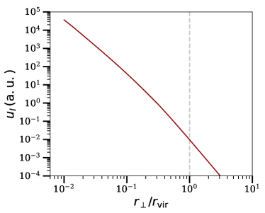
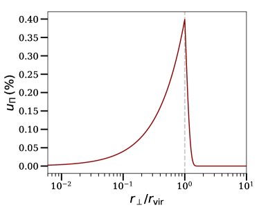
Figure 1: Projected profiles for the normalized total Ly$\alpha$ intensity (left panel), and the polarization fraction (right panel), with impact parameter. The vertical dashed lines denote the position of the virial radius.

Finally, the Ly$\alpha$ intensity profile can be written as

$$u_{I}(r_{\perp}|M,z)=\cfrac{S_{Ly\alpha}(r_{\perp})}{\int_{0}^{\infty}2\pi r_{\perp}{\rm d}r_{\perp}S_{Ly\alpha}(r_{\perp})}~{},$$ (27)

where the denominator acts as a normalization constant. Although the intensity profile can depend on halo mass and redshift, note that, with this derivation, the profile is independent on these quantities. The left panel in Figure 1 shows the resulting normalized profile, where the dashed line denotes the position of the virial radius, for reference.

3.2.2 Projected Profile for the Polarization Fraction

We model the projected profile of the polarization degree around the halos as a linear increase with impact parameter, followed by a steep decrease after peaking at the virial radius, as

$$u_{\Pi}(r_{\perp}|M,z)=\Pi_{\rm max}\times\left\{\begin{array}[]{ll}\cfrac{r_{\perp}}{r_{\rm vir}}&~{}r_{\perp}\leq r_{\rm rvir}(M,z)~{};\\[18.0pt] e^{\left[1-\left(r_{\perp}/r_{\rm vir}\right)^{5}\right]}&~{}r_{\perp}>r_{\rm rvir}(M,z)~{},\end{array}\right.$$ (30)

where $\Pi_{\rm max}=40\,\%$ is the maximum polarization fraction value at the virial radius, and $r_{\rm vir}(M,z)$ introduces the dependence on halo mass and redshift. The exact dependence on impact parameter is set arbitrarily, and variations are explored in § A in the Appendix. However, the shape and maximum polarization fraction value for this profile agree with those found in the radiative transfer simulations of Dijkstra & Loeb (2008) and Dijkstra & Kramer (2012). Furthermore, the profile is also broadly consistent with the simulations and observations of the polarization degree around the giant Ly$\alpha$ nebula LAB1 (Steidel et al., 2000) by Trebitsch et al. (2016) and Hayes et al. (2011), respectively. The right panel of Figure 1 illustrates this polarization fraction profile with impact parameter.

A strong assumption in our model is the sharp cut-off of the polarization signal at a given impact parameter. In reality, the polarization signal will extend out in the halo as long as the scattering of Ly$\alpha$ photons exists. At large impact parameter, however, the number of photons is largely reduced, the exact number depending on the slope adopted for the surface brightness, and only a few photons will contribute to the polarization signal. We explore the impact of a flat surface brightness profile, different values for the position of the cut-off, as well as a smoother cut-off slope in § A in the Appendix. Overall, as we will show, these changes have little effect on the one-halo terms of the power spectra of $\Pi$. In detail, the peak of the one-halo terms can be broader or narrower, but it is always well resolved at large multipole values. This is because the sharp shape of the one-halo terms at large $\ell$ arises mostly from the fact that the polarization fraction profile increases with impact parameter, contrary to the case of the surface brightness for which the signal decreases with distance. The sharp cut-off only impacts the shape of the low-multipole side of the power spectrum peaks.

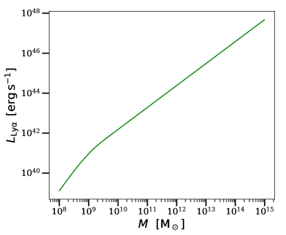
Figure 2: Redshift-independent relation between halo mass and Ly$\alpha$ luminosity described by Eq. 31. Note that the halo mass in this panel does not include the reduced Hubble constant term.

3.2.3 Halo Mass and Luminosity Relation

For our calculations, we use the Tinker et al. (2008) comoving halo-mass functions, covering the mass range $8\leq\log(M/{\rm M_{\odot}\,h^{-1}})\leq 15$.

To relate the halo mass and the Ly$\alpha$ luminosity, we use the expression derived by Inoue et al. (2018),

$$\frac{L_{\rm Ly\alpha}(M)}{10^{42}\,{\rm erg\,s^{-1}}}=\left(\frac{M}{\rm 10^{10}\,M_{\odot}}\right)^{1.1}\left[1-\mathrm{exp}\left(-{\frac{10M}{\rm 10^{10}\,M_{\odot}}}\right)\right]~{},$$ (31)

illustrated in Figure 2, and where the halo mass, $M$, now does not carry the reduced Hubble constant term. We use this expression for all redshifts in this work, although it was derived regarding observations at $5\lesssim z\lesssim 7$. Finally, the term $I(M)$ in the power spectrum equations corresponds to

$$I(M,z)=\frac{L_{\rm Ly\alpha}(M)}{4\pi\,(1+z)}~{},$$ (32)

which gives rise to the units for the $\nu I_{\nu}$ power spectra. The term $(1+z)^{-1}$ disappears when considering the specific intensity power spectra, $I_{\nu}$.

Our formalism assumes that all the Ly$\alpha$ photons produced via Eq. 31 will be observed, i.e., it ignores the effect of the escape fraction of Ly$\alpha$ photons. However, in our model, only dust contributes to the escape fraction value, not neutral gas. The neutral hydrogen gas can diffuse the Ly$\alpha$ emission far from the source via scattering, but the number of Ly$\alpha$ photons is conserved, contrary to the case of dust where the photons are mostly destroyed. Therefore, the use of Ly$\alpha$ escape fraction values that arise from measuring the removal of photons along the line of sight covering the central regions of galaxies should be avoided. For simplicity, we have also ignored the potential effect from a galaxy duty cycle. Because Ly$\alpha$ arises mostly from young stars, this effect may be considerable for massive halos with old stellar populations (e.g., Ouchi et al., 2018). Similarly, the effect of varying star-formation rates and efficiencies with redshift, as well as the dispersion around the mean values, could be important (see, e.g., Inoue et al., 2018; Sadoun et al., 2019; Laursen et al., 2019) but it is not accounted for in Eq. 31. We defer more detailed calculations to future work.

4 Results

This section presents the power spectra obtained with the formalism described above. In § 4.1, we show the power spectra obtained with our fiducial profile models. The distribution of halo masses contributing across redshifts, and for various multipoles, is presented in § 4.2. In § 4.3, we extract information about the polarization fluctuation in halos, and we show the cross power spectra for the fiducial models in § 4.4

For the calculations below, we consider a redshift depth of $\Delta z=0.5$, and assume that the redshift-dependent quantities are constant over this range. We note that this assumption is less valid at high redshifts, where the quantities evolve more rapidly with time, but we adopt it here for simplicity.

4.1 Power Spectra of Ly$\alpha$ Polarization

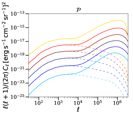
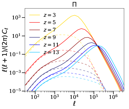
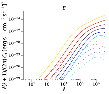
Figure 3: From top to bottom and left to right, the panels show the power spectra for the Ly$\alpha$ (total) intensity, $I$, polarized intensity, $\pazocal{P}$, polarization degree, $\Pi$, and $\tilde{E}$ modes at redshifts $z=3,\,5,\,7,\,9,\,11$ and $13$. The signal from $B$ modes is null by construction in our formalism. The sums of the one- and two-halo terms are denoted by the solid lines, and the two-halo terms are represented by the dashed ones. The power spectra of $\Pi$ and $\tilde{E}$ present sharp features (peaks or knees) whose positions depend on redshift. These peaks are related to the average size of the halos dominating the signal at a given redshift, while $I$ and $\pazocal{P}$ mostly only change the amplitude with redshift.

Figure 3 displays the power spectra for the Ly$\alpha$ polarization quantities $I$, $\pazocal{P}$, $\Pi$, and $\tilde{E}$, at redshifts $z=3,\,5,\,7,\,9,\,11$ and $13$, and for the fiducial parameters described in § 3.2. By construction, the $B$ mode signal is null in our formalism (see § 6). The figure shows that the spectra of the quantities $\Pi$ and $\tilde{E}$ yield more information on the halo population than that accessible by $I$ alone, due to the peaks (or knees) present in the power of these quantities (solid lines). The position of the one-halo peaks for $\Pi$ varies with redshift, from $\ell\sim 10^{4}$ at $z=3$ to $\ell\sim 10^{5}$ at $z=13$. The peak position indicates the average size of the halos dominating the power. Because there are few massive halos at high redshift, the power peaks at high $\ell$ values (small distances), while the increasing number of massive halos when decreasing redshift shifts the peak toward lower multipoles. Thus, the measurement of the peak position at a given redshift reveals the mean halo size (and in turn mass) dominating the polarization signal, provided that other potential effects are known. The position of the knees in the power spectra of $\tilde{E}$ is also related to the average size of the halos, although this relation is complex due to the Bessel function term in Eq. 2.2. None of these measurements is possible with intensity alone.

In § A in the Appendix, we address the impact of variations in the fiducial model parameters on the power spectra of the polarization quantities. We test changes in the spatial extent of the polarization signal, and in the intensity and polarization profile shapes. In general, these variations result in changes in the amplitudes of the power spectra, as well as in the positions of the peaks. Different behaviors are observed for different quantities and redshifts, which indicates that the analysis of various quantities and redshifts could be used to constrain the shape and extent of the real-space profiles more reliably than with one quantity (e.g., intensity) alone (see Sun et al., 2019, for a methodology to extract physical – small-scale – information from the intensity mapping power spectra).

The comparisons in § A in the Appendix show that the slope of the surface brightness profile in the halos is a crucial parameter for extracting polarization information from the power spectra. When the surface brightness profile is very steep, variations in the polarization profile (especially at large impact parameters) have little effect on the overall power spectra, because they are contributed by a small number of photons. This implies smooth one-halo peaks in general, for quantities other than $\Pi$. Variations in the polarization profile are most visible as effects in the power spectra of the polarization quantities when many photons contribute to the scales of interest. This occurs for surface brightness profiles that remain significantly flat out to the impact parameters corresponding to those scales. Large neutral gas regions illuminated by (various) bright sources, such as Ly$\alpha$ blobs or nebulae (e.g., Geach et al., 2016), as well as galaxy overdensities (e.g., Steidel et al., 2011; Matsuda et al., 2012), can keep extended and slowly decreasing surface brightness profiles, while isolated galaxies are expected to have steeper slopes, similar to our fiducial calculations, (e.g., Leclercq et al., 2017).

4.2 Halo Mass Distribution across Redshift

We assess here the halo masses that dominate the power at given multipoles and redshifts. For this calculation, we consider only the one-halo term, since it dominates the power at high $\ell$ values, where the peak of the power occurs in most cases. The halo-mass dependence is obtained via the partial derivative

$$\frac{{\rm d}\ln C_{\ell}(z)}{{\rm d}\ln M}\equiv\frac{M}{C_{\ell}(z)}\frac{{\rm d}C_{\ell}(z)}{{\rm d}M}=\frac{M\,\frac{{\rm d}n}{{\rm d}M}\,w^{2}(M)\,|\{\tilde{u},\tilde{E},\tilde{B}\}(\ell|M,z)|^{2}}{\int{\rm d}M\frac{{\rm d}n}{{\rm d}M}\,w^{2}(M)\,|\{\tilde{u},\tilde{E},\tilde{B}\}(\ell|M,z)|^{2}}~{},$$ (33)

where $\tilde{u}\equiv\tilde{u}_{\{I,\pazocal{P},\Pi\}}$, and $w$ is the same as in Eq. 6, with $w=1$ for $\tilde{E}$ and $\tilde{B}$.

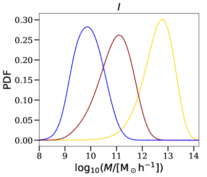
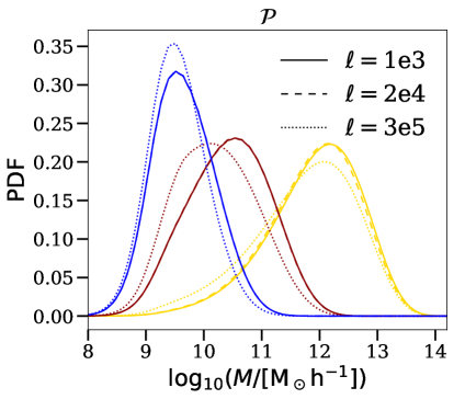
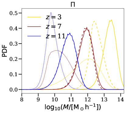
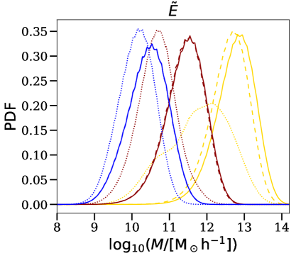
Figure 4: Halo mass contribution to the Ly$\alpha$ polarization quantities at redshifts $z=3$ (yellow), $z=7$ (dark red), and $z=11$ (blue), and at $\ell=10^{3}$ (solid lines), $\ell=2\times 10^{4}$ (dashed lines), and $\ell=3\times 10^{5}$ (dot-dashed lines). In general, the distributions shift toward lower halo masses as redshift increases due to the lower number of massive halos at early cosmic times. For the case of intensity, halo masses contribute equally to all $\ell$ in our models by construction and, therefore, differences between masses are not observed. The contribution of different halo masses to different multipoles is most significant for the quantities $\Pi$ and $\tilde{E}$.

Figure 4 shows the halo-mass distributions for the polarization quantities at three multipole and redshift values, $\ell=10^{3}$, $\ell=2\times 10^{4}$, and $\ell=3\times 10^{5}$, and $z=3,\,7$ and $11$, respectively. Overall, the distributions peak at higher halo masses when decreasing redshift, reflecting the increase in the number of massive halos at low redshift dictated by structure formation. The signal at high multipoles is dominated by less massive halos, due to the relation between halo mass and extent of the polarization signal in our formalism. This is most visible for the quantities $\Pi$ and $\tilde{E}$, whose power spectra in Figure 3 was already related to the average halo mass through the position of the peaks (knees) with redshift. For the case of intensity there is not dependence on multipole, because the normalized profile shape of intensity is independent of halo mass by construction in our formalism.

4.3 Polarization Fluctuations in Halos

We assess now the polarization information that can be retrieved from the ratio between the power spectra of $\pazocal{P}$ and $I$.

Let us consider here the halos as polarized point sources in the limit $\ell\to 0$, where the power spectra of the one-halo terms are approximated by those of the shot (Poisson) noise. In this case, the shot-noise power spectra for $I$ and $\pazocal{P}$ are proportional to (Tegmark & Efstathiou, 1996)

$$C_{\ell,I}^{\rm\,shot} \propto\int{\rm d}M\frac{{\rm d}n}{{\rm d}M}\,|I(M)|^{2}~{},$$ (34)

and

$$C_{\ell,\pazocal{P}}^{\rm\,shot} \propto\int{\rm d}M\frac{{\rm d}n}{{\rm d}M}\,|\pazocal{P}(M)|^{2}~{},$$ (35)

respectively. Similarly, the $\pazocal{P}$ power spectrum for the halos with polarization fraction $\Pi$ can be expressed as (Lagache et al., 2019)

$$C_{\ell,\pazocal{P}}^{\rm\,shot}(\Pi) \propto\Pi^{2}\int{\rm d}M\frac{{\rm d}n}{{\rm d}M}\,|I(M)|^{2}~{},$$ (36)

where we have assumed that $\pazocal{P}(M)\equiv\Pi\,I(M)$, with $\Pi$ independent on halo mass. Then, the power spectrum of the entire distribution of polarization fraction values, $P(\Pi)$, equates

$$C_{\ell,\pazocal{P}}^{\rm\,shot} =\int_{0}^{1}P(\Pi)\,C_{\ell,\pazocal{P}}^{\rm\,shot}(\Pi)\,{\rm d}\Pi=\langle\Pi^{2}\rangle\,C_{\ell,I}^{\rm\,shot}~{},$$ (37)

where $\langle\Pi^{2}\rangle$ denotes the mean squared value of the polarization fraction in halos. Thus, the ratio of the one-halo term power spectra of $\pazocal{P}$ and $I$ in the limit $\ell\to 0$ gives information about the polarization fluctuation in the entire halo population.

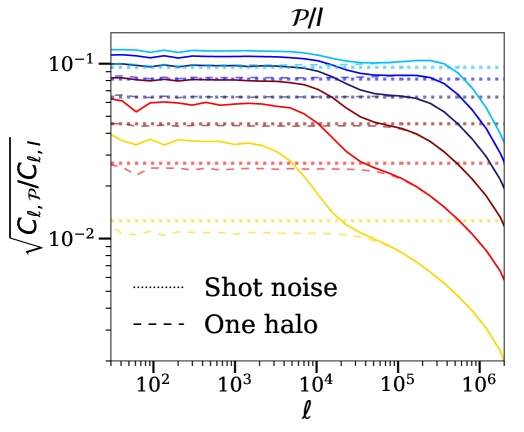
Figure 5: Ratio between the power spectra of $\pazocal{P}$ and $I$ at the redshifts of our calculations. From top to bottom, the lines denote the redshifts $z=13,$ 11, 9, 7, 5, 3. The solid lines denote the the square root of the ratio, and the dashed lines account for the case of the one-halo terms alone. The dotted horizontal lines show the square root of the ratio between the shot-noise power of $\pazocal{P}$ and $I$, i.e., ${\langle\Pi^{2}\rangle}^{1/2}$, which denotes the r.m.s of the polarization fluctuation in halos. This ratio broadly compares to the one-halo term values in the limit $\ell\to 0$, the differences arising from assuming a polarization fraction per halo independent on halo mass. The increase of ${\langle\Pi^{2}\rangle}^{1/2}$ with redshift is due to the more compact signal (less number density of massive halos) at earlier times. The steepness of the decay of the one-halo terms with redshift is an indicator of the distribution of $\Pi$ values. At high redshifts, most halos are small, and thus the distribution of $\Pi$ is narrow, which yields a steep slope. Instead, a broader distribution of halo sizes and, therefore, of $\Pi$ values at lower redshifts, results in a smoother decay of the ratio. The same dependence on halo sizes can be inferred from the position from where the one-halo terms begin their rapid decrease toward high $\ell$ values.

Figure 5 shows the ratio between the power spectra of $\pazocal{P}$ and $I$ at the redshifts of our calculations, from top to bottom, $z=13,$ 11, 9, 7, 5, 3. The solid lines denote the square root of the ratio, and the dashed lines represent the one-halo terms alone. The dotted horizontal lines show the square root of the ratio between the shot-noise power of $\pazocal{P}$ and $I$ (Eq. 37), i.e., ${\langle\Pi^{2}\rangle}^{1/2}$, which is the r.ms. fluctuation of polarization fraction values between halos. For the case of measured power spectra, the value of ${\langle\Pi^{2}\rangle}^{1/2}$ can be estimated from the flattening of the one-halo terms, where the dashed lines approximate the dotted lines. The differences between the flattening of the one-halo term and the ratio of power spectra arises from our assumption that the halo polarization fraction is independent on the halo mass. The increase of fluctuations with redshift, from ${\langle\Pi^{2}\rangle}^{1/2}\sim 0.01$ at $z=3$ to ${\langle\Pi^{2}\rangle}^{1/2}\sim 0.1$ at $z=13$, arises from the smaller average halo size at early times than at low redshift. In our formalism, the polarization fraction increases quickly with impact parameter in small sources because of the small virial radius (Eq. 30), and it is more sensitive to variations of this slope, and in turn of the halo mass. The reduced variation of ${\langle\Pi^{2}\rangle}^{1/2}$ at high redshifts indicates that the distribution of halo sizes is similar at these epochs, while the distribution of halo sizes evolves more rapidly at low redshift.

Additional information can be inferred from the slope of the decay of the one-halo terms toward high multipoles in Figure 5. A steep decay, or a pronounced knee, signals that the polarization degree profiles are similar for the entire halo population. The steep decay of the power at high redshift indicates that the halos have a narrower size distribution compared to low redshift, where the decay shape is smoother. Note that this redshift evolution arises due to the dependence of the polarization fraction signal with halo size, through the virial radius, in our formalism. Finally, the position of the knee in the one-halo term of the power spectra can be used as an estimator of the average size for the polarization signal, similarly to the case in the auto power spectra of $\Pi$ and $\tilde{E}$ previously discussed in § 4.1.

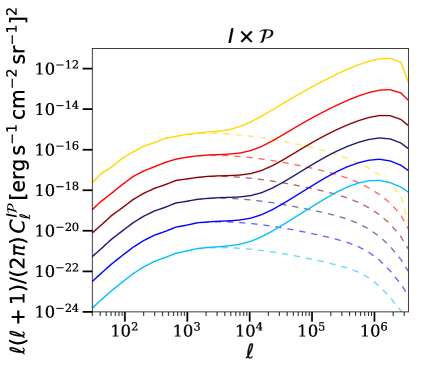
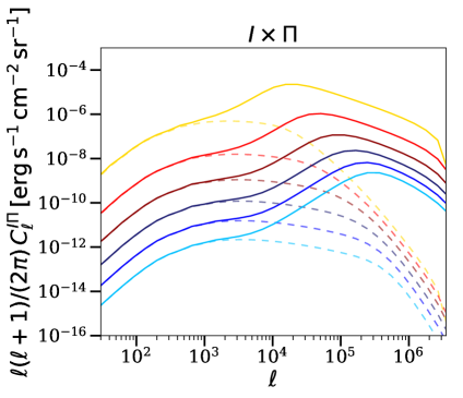
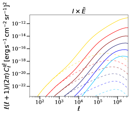
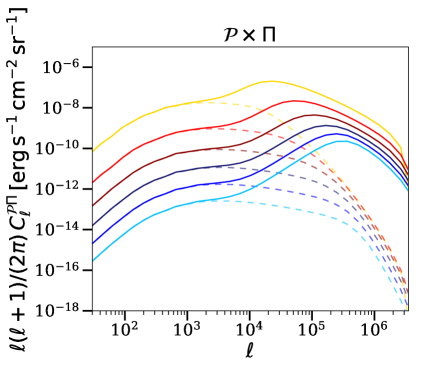
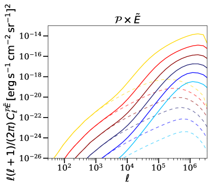
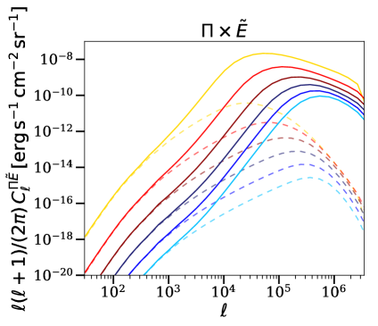
Figure 6: Cross power spectra for the polarization quantities $I$, $\pazocal{P}$, $\Pi$, and $\tilde{E}$, and for the fiducial model parameters.

4.4 Cross Power Spectra of Ly$\alpha$ Polarization

Figure 6 shows the cross power spectra between the quantities $I$, $\pazocal{P}$, $\Pi$, and $\tilde{E}$, taking into account the fiducial model parameters. Overall, the cross power spectra that consider the polarization fraction, $\Pi$, present the sharpest peaks in the one-halo terms, which makes their identification easier than in other cases. Furthermore, the position of the peaks changes with redshift, which indicates that the position is connected to the average size of the polarization signal, i.e., the dominant size of the halos in our formalism.

5 Detectability Estimates

We perform calculations for the detectability of the Ly$\alpha$ polarization signal below, and we discuss the impact of foregrounds in § 5.1.

This section presents estimates on the detectability of the power spectra, assuming that the signal is Gaussian, for simplicity. In practice, the signal may be highly non-Gaussian due to the small (non-linear) galaxy scales where the polarization is maximized. In this later case, a full covariance matrix calculation would be required (see, e.g., Komatsu & Seljak, 2002).

For a Gaussian statistic, the S/N can be computed following Knox (1995) as

$$S/N^{2}\,(\ell)=\frac{{C_{\ell}}^{2}}{(\Delta C_{\ell})^{2}}~{},$$ (38)

where

$$(\Delta C_{\ell})^{2}\equiv{\rm Var}(C_{\ell})=\frac{2}{2\ell+1}\frac{1}{f_{\rm sky}}\left(C_{\ell}+w^{-1}e^{\ell^{2}\,\sigma_{b}^{2}}\right)^{2}~{}.$$ (39)

The first summand in the above expression describes the sample (cosmic) variance, and the second one represents the instrumental (thermal) noise, where $W_{\ell}=e^{\ell^{2}\,\sigma_{b}^{2}}$ is the window function for a Gaussian beam of size $\sigma_{b}$, and $f_{\rm sky}$ denotes the fraction of the sky covered by the observations. The term

$$w\equiv\left(\sigma_{\rm pix}^{2}\,\Omega_{\rm pix}\right)^{-1}~{}$$ (40)

represents a weight per solid angle, and $\sigma_{\rm pix}$ and $\Omega_{\rm pix}$ are the pixel uncertainty and solid angle, respectively. The pixel uncertainty can be calculated as

$$\sigma_{\rm pix}=\frac{s}{\sqrt{t_{\rm pix}}}~{},$$ (41)

where $t_{\rm pix}=(N_{\rm feeds}\,\Omega_{b}/4\pi\,f_{\rm sky})\,t_{\rm survey}$ is the observing time per pixel, with $N_{\rm feeds}$ denoting the number of spectro-polarimeters (spatial channels) simultaneously observing the sky, and $t_{\rm survey}$ is the total observing time of the experiment. The numerator in Eq. 41 describes the sensitivity, and can be accounted for via the noise equivalent flux density (NEFD) as (Sun et al., 2019)

$$s=\frac{\rm NEFD}{\Omega_{b}}~{},$$ (42)

where

$$\Omega_{b}=\Theta_{\rm FWHM}^{2}=(2\sqrt{2\ln 2}\,\sigma_{b})^{2}~{}$$ (43)

denotes the beam solid angle, and $\Theta_{\rm FWHM}$ describes the full-width at half maximum for the beam.

For the case of the polarization degree, $\Pi$, we calculate the uncertainty by accounting for the propagation of the uncertainties in $I$ and $\pazocal{P}$ as

$$\cfrac{\Delta C_{\ell,{\Pi}}}{C_{\ell,\Pi}}=\sqrt{\left(\cfrac{\Delta C_{\ell,{\pazocal{P}}}}{C_{\ell,{\pazocal{P}}}}\right)^{2}+\left(\cfrac{\Delta C_{\ell,{I}}}{C_{\ell,I}}\right)^{2}}~{}.$$ (44)

This is motivated by the fact that, in practice, $\Pi$ will be derived from the separate measurements of these two quantities. This approach yields an uncertainty higher by a factor $\sim 1.5$ compared to that from simply using Eq. 39.

We estimate the sensitivities required to detect the polarization signal, and compare them to the sensitivity levels of real ground- and space-based instruments. The ground-based case is compared to the HETDEX experiment (Hill et al., 2008), and the space-based estimate considers CDIM (Cooray et al., 2019). None of these instruments, however, are (presently) designed to perform polarization observations.

Briefly, HETDEX is a ground-based experiment, equipped with a spectrograph and $150$ integral field units (IFUs; Hill et al., 2014), that will perform a blind wide-field spectroscopic survey. HETDEX is expected to detect $\sim 0.8$ million LAEs in the redshift range $1.9<z<3.5$, and over an area of $\sim 400$ ${\rm deg^{2}}$ on the sky for three years. However, Fonseca et al. (2017) already noted that HETDEX can also be used for Ly$\alpha$ intensity studies, because the IFUs will take data from several patches of the sky blindly, i.e., regardless of the number or position of known Ly$\alpha$ sources in them. This data, therefore, will contain a number of bright sources, but will also include the faint diffuse emission from undetected and/or extended objects that are the target of intensity mapping. Furthermore, the sensitivity of HETDEX is designed to detect the Ly$\alpha$ emission line flux at high spectral resolution, i.e., over a redshift depth of $\Delta z\approx 0.006$, in order to resolve the Ly$\alpha$ line profile. Because this high spectral resolution is not required for intensity studies (e.g., we consider here $\Delta z=0.5$), in practice, we can add the flux from many spectral HETDEX bins and thus reduce the pixel uncertainty, $\sigma_{\rm pix}$, by a factor of $\sqrt{N_{z}}\approx 9$, where $N_{z}$ is the number of spectral bins.

CDIM is a proposed intensity mapping space observatory designed to study the epoch of cosmic reionization via the Ly$\alpha$ emission in the wavelength range $0.75\lesssim\lambda/\mu{\rm m}\lesssim 7.5$, covering a sky area of $\sim 300$ ($\sim 15$) ${\rm deg^{2}}$ for a wide (deep) survey, and with a spectral resolution of $R=300$.

Table 1 quotes the parameters adopted for our calculations with a hypothetical ground-based Ly$\alpha$ polarization experiment, Lyapol-G, and a space-based experiment, Lyapol-S. The first column refers to the experiment, and the second column is the spectral resolution assumed in the calculations. The third column quotes the pixel uncertainty resulting from the observing times and individual characteristics of the experiments at the redshift of Ly$\alpha$ stated in the fourth column. The fifth and sixth columns are the pixel and beam solid angles, respectively. The fraction of the sky covered by the surveys is quoted in the seventh column. Overall, the sensitivities quoted in the third column of Table 1 are a factor of $\sim 10$ (for Lyapol-G) and of $\sim 100$ (for Lyapol-S) higher than the nominal values of HETDEX and CDIM, respectively. Although the total intensity can be detected at the nominal values for these instruments, we show that the higher sensitivities are required to reach the polarization signal in a broad redshift range. We have also reduced the pixel and beam sizes for Lyapol-S compared to the case of CDIM in order to achieve the small physical scales where the polarization power is significant at high redshifts.

=-1in

Table 1: Instrumental Parameters

Instrument	$R$	$\sigma_{\rm pix}\,{[\rm erg\,s^{-1}\,cm^{-2}\,sr^{-1}]}$	$z_{\rm Ly\alpha}$	$\Omega_{\rm pix}\,{\rm[{arcsec}^{2}]}$	$\Omega_{b}\,{\rm[{arcsec}^{2}]}$	$f_{\rm sky}$
Lyapol-G	$700$	$2.6\times 10^{-6}$	$3$	$5.40$	$9$	$0.010$
Lyapol-S	$300$	$1.6\times 10^{-7}$	$9$	$0.50$	$2$	$0.008$

Figure 7 displays the uncertainties for the fiducial power spectra of Figure 3 at redshifts $z=3$ (yellow lines) and $z=9$ (blue lines) with the parameters of Lyapol-G and Lyapol-S described in Table 1, respectively, and considering a redshift depth $\Delta z=0.5$ in all cases. The dots represent the positions where the variance is calculated, and the shaded areas represent the uncertainty, obtained by simply interpolating between the values in the points. Overall, this figure shows that the amount of signal collected by the large redshift depth ($\Delta z=0.5$) enables measurements of the power spectra between $\ell\sim 10^{2}$ and $\ell\sim 10^{5}$ for all the quantities but $\tilde{E}$. The steep decay and low values of the $\tilde{E}$ signal toward low multipoles does not allow detecting this power even at the lowest redshift. The peak of the power at multipole values $\sim 10^{5}$ is high enough to be detected, but this would require a smaller beam and pixel sizes than the ones quoted in Table 1.

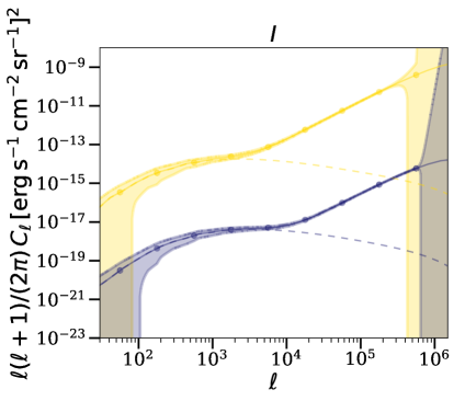
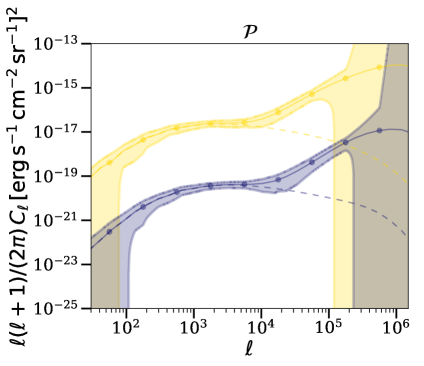
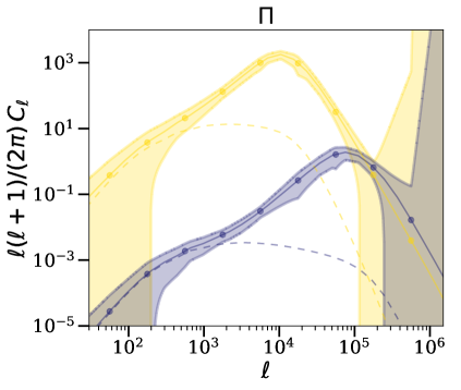
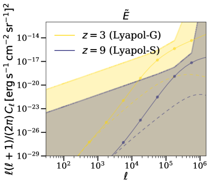
Figure 7: Detectability estimates for the fiducial power spectra of Figure 3 at redshifts $z=3$ (yellow lines) and $z=9$ (blue lines) with the parameters of Lyapol-G and Lyapol-S described in Table 1, respectively, and considering a redshift depth $\Delta z=0.5$ in all cases. The dots represent the positions where the variance is calculated, and the shaded areas represent the uncertainty in the power by interpolating between points. The amount of signal collected by the large redshift depth enables precise measurements of the power spectra between $\ell\gtrsim 10^{2}$ and $\ell\sim 10^{5}$ for all but the $\tilde{E}$ quantities. The low values of the $\tilde{E}$ power at small multipoles and the beam and pixel sizes are the reasons behind the non detection.

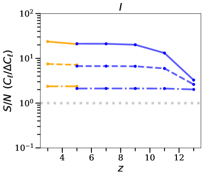
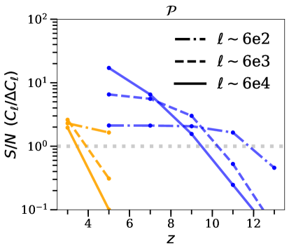
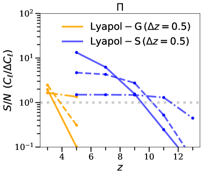
Figure 8: S/N estimates for three multipole values, and for all but the $\tilde{E}$ polarization quantities. The orange and blue lines denote the ground-based Lyapol-G and space-based Lyapol-S setups, respectively, with a redshift depth of $\Delta z=0.5$. We have used the same sensitivity for $z=5$ and $z=3$ for Lyapol-G. The sensitivity evolution of Lyapol-S with redshift is taken from the CDIM deep case reported in Cooray et al. (2019), rescaled to our value at $z=9$ in Table 1.

Figure 8 illustrates the S/N for the two instrumental setups at three multipole values, and for all but the $\tilde{E}$ polarization quantities. The orange and blue lines denote the ground-based Lyapol-G and space-based Lyapol-S setups, respectively, with a redshift depth of $\Delta z=0.5$. We have assumed the same sensitivity for Lyapol-G at $z=5$ and $z=3$. The evolution of the sensitivity with redshift for the case of Lyapol-S is taken from the CDIM ‘deep’ case shown in the middle panel of figure 2 in Cooray et al. (2019), rescaled to our value at $z=9$ in Table 1. The instrument sensitivity increases by a factor of $\sim 3$ from redshift $z\sim 5$ to $z\sim 13$, but this is counterbalanced by the fact that the number of spectral channels that cover $\Delta z=0.5$ decreases with redshift at a fixed spectral resolution. Overall, the S/N for the total intensity remains fairly constant at all three multipoles up to $z\sim 9$, beyond which the instrumental sensitivity suppresses the signal rapidly, from the highest to the lowest multipoles. Because the power of the polarized intensity is a few orders of magnitude fainter than that for the total intensity, the steep decrease in S/N appears already at redshift $z\sim 5-7$. The turnover of the $\Pi$ power spectra is detectable (S/N$\sim 2-3$) at $z=3$ with Lyapol-G, and up to $z\sim 9$ with Lyapol-S.

In summary, these simple estimates suggest that the detection of Ly$\alpha$ polarization up to the early times of reionization requires sensitivities higher than those of current and near-future experiments. We discuss in the next section the sources of foreground contamination that need to be taken into account for these observations.

5.1 Foregrounds

The major source of foreground polarization detectable from the ground at wavelengths of $\lambda\sim 1\mu$m is the atmospheric Rayleigh-scattered radiation from the Moon and the stars (Glass, 1999). From space, the atmospheric component is significantly reduced, and the primary contamination arises from starlight scattered by the Milky Way dust (Sparrow & Ney, 1972; Arai et al., 2015). These contributions, however, present a smooth spectrum with a known frequency dependence, which one could try to model and subtract from the observations (Brandt & Draine, 2012). Furthermore, the use of cross-correlations would allow the identification of the foreground signal, because the latter would not be correlated with the sources (galaxies) of Ly$\alpha$ polarization of interest.

A significant benefit of using polarized emission for the detectability, compared to using total emission, is the reduced impact from interlopers. When considering polarized radiation, emission at a given frequency that redshifts into the detection window of Ly$\alpha$, will not be misidentified as Ly$\alpha$ unless it is polarized. This improvement enables one to use large redshift depths for the integration of signal, and thus increase the S/N, without suffering from extreme interloper contamination.

A source of foreground contamination for the polarization signal of interest, may be the polarized H$\alpha$ radiation originating from Raman-scattered Ly$\beta$ radiation (Lee & Ahn, 1998, see also the case of scattered Ovi by neutral hydrogen in Nussbaumer et al. 1989). This process, however, occurs at column densities typical of that in the interstellar medium and, therefore, the signal would be, in most cases, compact and in the core of the sources. If this process happens below the spatial resolution of the detector, the average polarization signal would be null. However, if it is extended, it may be included in the observations. The polarization signal from the core of objects such as high-redshift radio galaxies (e.g., Cimatti et al., 1998; Vernet et al., 2001) or Seyfert II galaxies, is also expected to be compact and, therefore, to not introduce significant contamination into the measurements. Finally, in Mas-Ribas & Hennawi (2018), we demonstrated that the radiation from a hyperluminous quasar that is Thomson scattered by the free electrons (or scattered by dust) in the circumgalactic medium of the host galaxy can be detectable. Even though this signal can extend well out into the halo, these bright sources are rare and identifiable (maskable) to avoid contamination from electron scattering on the Ly$\alpha$ polarization signal of interest here.

6 Ly$\alpha$ $B$ Modes as Probes of Halo Anisotropy, Gravitational Lensing and Faraday Rotation

The Ly$\alpha$ $B$ mode power in our formalism is null, because we have considered a radially symmetric (isotropic) polarization signal around the halos. In reality, however, the Hi distribution in galaxy halos can present a complex and inhomogeneous geometry, and the emission of Ly$\alpha$ radiation from the source can be highly anisotropic, which will result in patterns departing significantly from the idealized isotropic case. Therefore, a Ly$\alpha$ $B$ mode signal is expected to arise from actual galaxies, where the $B$ mode amplitude will be an indicator of the amount of ‘polarization anisotropy’ in the halos. Measurements of the global Ly$\alpha$ $B$ and $E$ mode signals at various redshifts could be used as indicators of the evolution of the average inhomogeneity and anisotropy of halos over time. This quantification, in turn, might be a tracer of the major physical processes driving galaxy evolution, such as merging rates, or feedback effects impacting the properties of the gas in the halos at different redshifts.

Other sources of Ly$\alpha$ $B$ modes are the effects of gravitational lensing (Zaldarriaga & Seljak, 1998), and Faraday rotation (Kosowsky & Loeb, 1996; Kosowsky et al., 2005), which convert the propagating Ly$\alpha$ $E$ modes into $B$ modes. For a high number density of Ly$\alpha$ polarization sources, covering a large fraction of the sky, weak gravitational lensing $B$ modes may be considerable and of interest (e.g., Foreman et al., 2018). Furthermore, because the Ly$\alpha$ sources exist at all redshifts, one could perform a tomographic analysis of the lensing signal, separating the contribution of different redshift bins. However, we expect the lensing signal to be small when the fraction of the sky covered by sources is small, owing to the small size of the polarization signal in the halos. In this case, however, one might be able to investigate the galaxy lensing effects by measuring the shear introduced to the shape of the $E$ modes around individual objects. The impact from Faraday rotation is uncertain, because it depends strongly on the magnetic fields, as well as on the distribution of matter in the Milky Way and the intergalactic medium, all quantities difficult to constrain with precision. However, De & Tashiro (2014) found that the impact of Faraday rotation on pre-reionization polarized 21cm radiation is very important due to the large wavelength of this radiation. Because Faraday rotation depends on the square of the wavelength, this effect would be about $(10^{5})^{2}$ times smaller for Ly$\alpha$ than for 21cm, albeit the other parameters remain the same for both frequencies. Finally, $B$ modes might also arise from the clustering or merging, as well as overlap, of halos, which is beyond the capabilities of the halo model approach.

In addition to these ‘physical’ sources of Ly$\alpha$ $B$ modes, it is also possible that there is a contaminant signal arising from ‘ambiguous’ modes (e.g., Lewis et al., 2002; Bunn et al., 2003). Ambiguous modes appear when only a fraction of the sky is observed. In this case, the decomposition of the polarization signal is non-local and non-unique, and therefore modes that are simultaneously divergence free (like $B$ modes) and curl free (like $E$ modes) appear. In other words, it is not clear whether the power of these modes is contributed by $E$ or $B$. This effect can be especially significant for the case of a Ly$\alpha$ $B$ mode measurement, because we expect the $B$ modes to be subdominant compared to $E$ modes. The level of leakage between $E$ and $B$ modes may be significant compared to the signal expected for the $B$ modes, and it can therefore misguide the interpretation of the observations.

7 Future Work

In our calculations, we have not included the potential effect of Population III galaxies, which would result in a significant increase of the Ly$\alpha$ emissivity compared to our fiducial calculations that consider normal (Population II) galaxies (e.g., Raiter et al., 2010; Mas-Ribas et al., 2016). This effect, however, would be significant for the (global) power spectra calculations at redshifts above $z\gtrsim 10-15$, where the average star-formation rate may be dominated by Population III galaxies, as suggested by recent numerical (Jaacks et al., 2018), as well as (semi-)analytical (Mebane et al., 2018; Mirocha et al., 2018) star-formation calculations.

Rybicki & Loeb (1999) suggested that an important source of Ly$\alpha$ polarization other than galaxies, even before cosmic reionization, could be the scattering of photons with intergalactic (IGM) neutral hydrogen gas moving with the Hubble flow. This polarization can reach degrees of polarization as high as $\sim 70\,\%$, although (Dijkstra & Loeb, 2008) noted that this would be the case for gas beyond $\sim 10$ virial radii from galaxies. The ‘static’ intergalactic gas closer to galaxies would reach lower polarization degrees, on the order of $\lesssim 7\,\%$. However, the gas at a few virial radii may be inflowing toward the halo center due to gravitational collapse, which may introduce polarization levels of a few tens of percent. This IGM Ly$\alpha$ polarization component can be important at redshifts above $z\sim 6$, where the IGM may still present large neutral gas regions. We will investigate the impact of this intergalactic polarization via analytical and numerical calculations in future work.

An important aspect that needs to be revisited in future work is the effect of performing cross correlations between the polarization signals and other tracers of cosmic structure and/or line emission at other frequencies (e.g., galaxies, quasars, or 21 cm, CO, Cii, and H$\alpha$ emission). For example, because the Ly$\alpha$ polarization signal is high at small (galaxy) scales, the cross correlation of Ly$\alpha$ polarization with galaxies could be used to enhance the detectability at those scales.

8 Conclusions

We have presented an analytical formalism of Ly$\alpha$ polarization, arising from the scattering of photons with neutral hydrogen gas around galaxies, for intensity mapping studies. We have used the halo-model formalism, as well as Ly$\alpha$ profiles based on simulations and observations, for modeling the signal. We have estimated the auto and cross power spectra of the Ly$\alpha$ quantities total intensity, $I$, polarized intensity, $\pazocal{P}$, polarization fraction, $\Pi=\pazocal{P}/I$, and the astrophysical Ly$\alpha$ $E$ and $B$ modes, introduced here for the first time in galaxy studies, and derived from the CMB formalism. The dependence on model parameters and the impact of variations in their values has been investigated, as well as the detectability of the power spectra for the aforementioned quantities, considering the redshift range $3\lesssim z\lesssim 13$. The main findings of this work are as follows:

1. The power spectra of the polarization quantities $\Pi$ and $E$ present sharper features than the power spectra of $I$ and $\pazocal{P}$ in general, especially for the one-halo terms (Figures 3 and 6). The position of the one-halo peaks of $\Pi$ and $E$ depends on redshift, and it is related to the average halo size (and mass) dominating the signal at a given time.

2. The ratio between the power spectra of the polarized intensity and the total intensity gives information of the polarization fluctuations between halos. Furthermore, the distribution of sizes for the polarization signal can be obtained from the ratio of the one-halo terms at high multipoles. Finally, the evolution of the polarization fluctuations with redshift indicates the dependence of the polarization signal with halo size (Figure 5).

3. The signal from Ly$\alpha$ $B$ modes is null by construction in our formalism, because we consider symmetry around the halos. In real data, however, a $B$ mode signal is expected to arise from the anisotropy in the halo gas distribution and the radiation field. The combined measurements of Ly$\alpha$ $E$ and $B$ modes for various redshifts will yield information about the physical properties and the evolution of cold gas in halos (§ 6).

4. Variations in the amplitudes and shapes of the Ly$\alpha$ profiles, especially in the slope of the surface brightness profile, produce different changes for the power spectra of different polarization quantitites, and for different redshifts. Comparisons between various quantities, and at various redshifts, enables one to extract the physical characteristics (slope and extent) of the real-space Ly$\alpha$ profiles (§ A in the Appendix).

5. The detectability of the polarization signal requires improvements in the sensitivity of current ground- and space-based experiments by factors between $\sim 10-100$, depending on redshifts and experiments (Figures 7 and 8, and § 5). Foreground contamination from the atmosphere, and Milky Way dust-scattered radiation, is expected to be important and needs to be modeled and removed (§ 5.1).

6. The contamination from interlopers is expected to be smaller when considering polarized radiation than total radiation, because the contaminant radiation needs to also be polarized to impact the measurements.

We have shown that the use of polarization in intensity mapping studies enables extracting more physical information about the galaxies and their environments than total emission alone. This first work has presented the general formalism, which will be extended, as well as applied to specific cases, via analytical and numerical calculations in coming studies.

Below, § A shows the impact on the power spectra of variations in the fiducial model parameters.

Appendix A Dependences on Model Parameters

We explore below the impact of variations in the model parameters on the fiducial power spectra of Figure 3. We first test changes in the extent of the polarization signal, out to three and five virial radii, as well as for the hypothetical case for which all halos show the same polarization extent. We then assess changes in the shape of the surface brightness and polarization profiles.

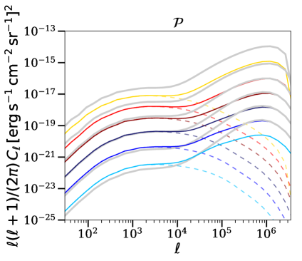
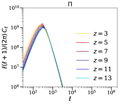
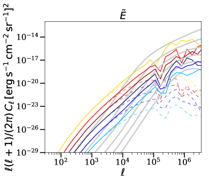
Figure 9: Power spectra estimates adopting a position for the maximum polarization fraction at three virial radii (color lines), compared to the fiducial calculations that consider one virial radius (gray lines). In general, the spectra for $\pazocal{P}$ and $\tilde{E}$ show a higher power at low multipoles and a lower one at large $\ell$ values compared to the fiducial case, and the one-halo term peak in the fiducial calculation is now smoothed out. The power for $\Pi$ shows a sharp peak corresponding to the two-halo term at $\ell\sim 10^{2}-10^{3}$, whose amplitude is now more than three orders of magnitude above the noise (not visible). The power does not change for the total intensity, $I$, because the signal does not depend on the polarization fraction.

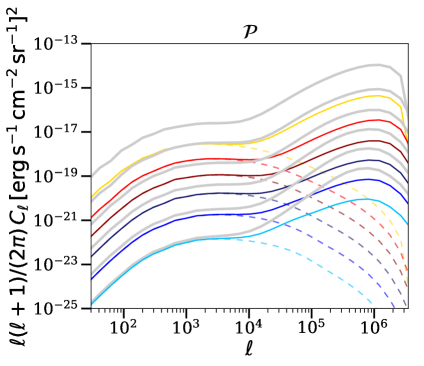
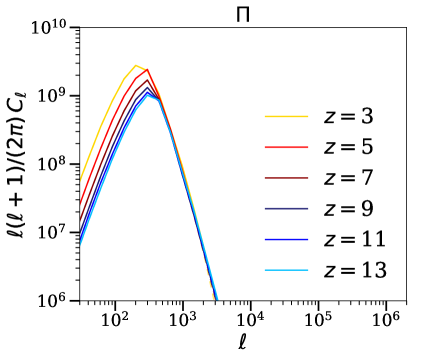
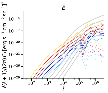
Figure 10: Same as Figure 9, but with the maximum polarization fraction value now at five virial radii.

1. Extent of the polarization signal. Our fiducial model assumes that the maximum polarization fraction value occurs at the virial radius of the halos, and it becomes zero rapidly after that position. Figure 9 illustrates the impact of shifting the peak value out to three virial radii (colored lines) on the fiducial power spectra of Figure 3 (gray lines). For the case of the total intensity, this produces no differences because $I$ does not depend on the polarization fraction. For $\pazocal{P}$ and $\tilde{E}$, the shape of the power spectra is smoother. The major impact of changing the extent of polarization is visible in the power spectra of $\Pi$ (bottom left panel), which is now characterized by a sharp feature at $\ell\sim 10^{2}-10^{3}$.

   Figure 10 shows the case of shifting the maximum polarization fraction value out to five virial radii, which results in a similar behavior as for the case of three virial radii just discussed.

   We also test the impact of a fix size for the polarization fraction profile, for comparison. Figure 11 shows the power spectra obtained by considering the maximum polarization degree for all halos occurring at an (arbitrary) impact parameter of $r_{\perp}=50$ comoving kpc ${\rm h^{-1}}$. At the lowest redshifts, the one-halo terms of $\pazocal{P}$ and $\tilde{E}$ are enhanced compared to the fiducial case, because now all halos are small instead of distributed in a broad range of sizes. Because all halos are typically small at high redshifts, the fix (small) impact parameter power spectra do not differ significantly from the fiducial calculations. The largest impact is visible as a reduction of the power spectra of $\Pi$ at the lowest redshifts. All the spectra now peak at the same position, because the extent of the polarization signal is constant.

   

   

   

   

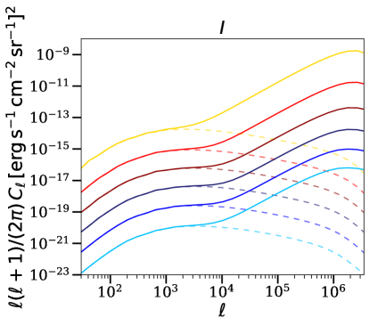
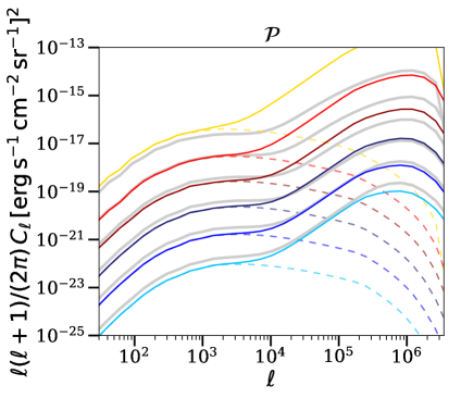
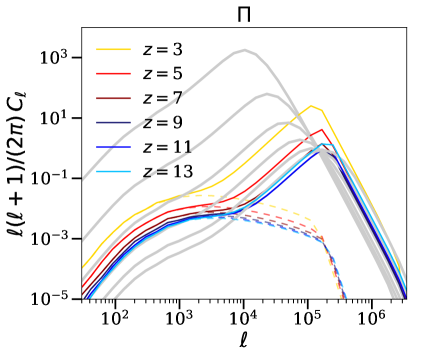
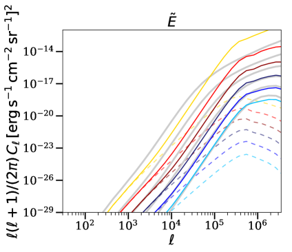
   Figure 11: Same as Figure 9, but fixing now the position of the maximum polarization fraction to a projected distance of $r_{\perp}=50$ comoving kpc ${\rm h^{-1}}$ from the center for all halos.

   

   

   

   

   

   

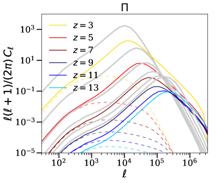
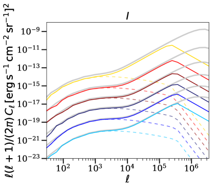
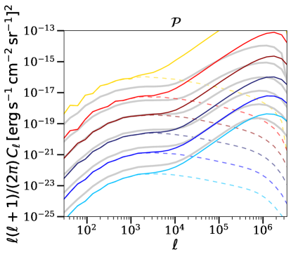
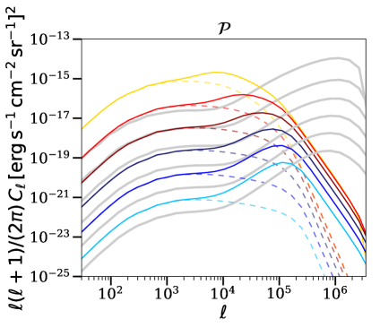
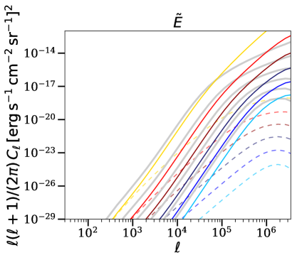
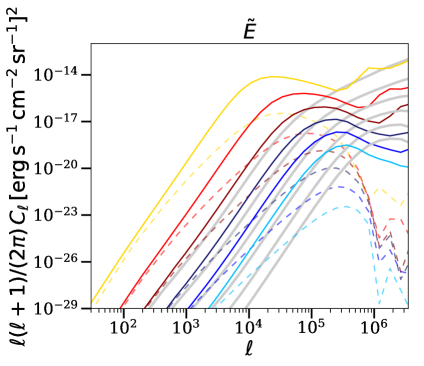
   Figure 12: Left column: Power spectra considering a constant polarization fraction profile with a value of $10\,\%$, out to one virial radius (colored lines). Right column: Power spectra for the case of a flat surface brightness profile extending out to three virial radii (colored lines). For comparison, the fiducial power spectra of Figure 3 are shown as gray lines.

2. Surface brightness and polarization fraction profile shape. The right panels in Figure 12 show the power spectra adopting a flat surface brightness profile extending out to three virial radii of the halos (color lines). The power spectra for intensity (top right panel) show a one-halo term peak at $\ell\sim 4-5\times 10^{5}$. For $\pazocal{P}$ (middle right panel), the power previously in the one-halo terms is transferred to lower multipoles, especially at low redshifts. The power spectra of $\tilde{E}$ (bottom right panel), in general, are shifted toward lower $\ell$ compared to the fiducial case, and the knees become sharp peaks easier to identify, and whose position depends on redshift similarly to $\Pi$.

   The left panels in Figure 12 display the comparison between the fiducial power spectra (gray lines), and, from top to bottom, those for $\Pi$, $\pazocal{P}$, and $\tilde{E}$, resulting from considering a constant polarization fraction value of $10\,\%$, from the center of the halo out to one virial radius (color lines). The power spectra of $\Pi$ present lower amplitudes than the fiducial calculation, while the power spectra of $\pazocal{P}$ and $\tilde{E}$ show milder variations, mostly resulting in steeper one-halo terms at the lowest redshifts.

   

   

   

   

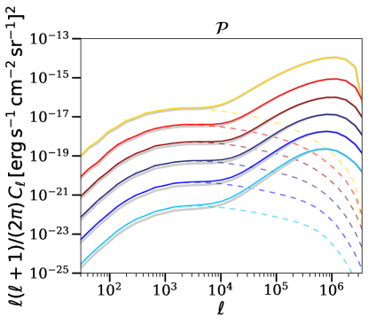
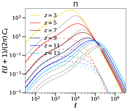
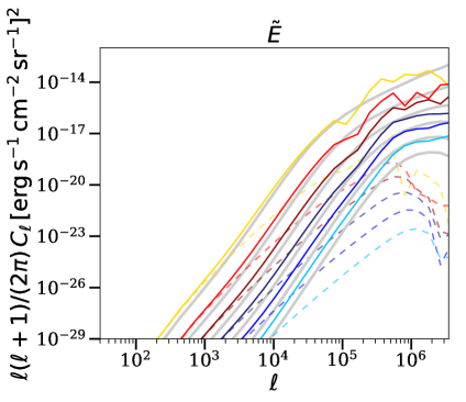
   Figure 13: Power spectra considering a slow decay, proportional to $\mathrm{exp}\left(1-r_{\perp}/r_{\rm vir}\right)$, of the polarization fraction beyond one virial radius (color lines). For comparison, the gray lines denote the fiducial power spectra of Figure 3, with a decay proportional to ${\rm exp}[1-(r_{\perp}/r_{\rm vir})^{5}]$.

   We have also tested the impact of a polarization fraction profile that decays slowly after the virial radius, proportional to $\mathrm{exp}\left(1-r_{\perp}/r_{\rm vir}\right)$ instead of ${\rm exp}[1-(r_{\perp}/r_{\rm vir})^{5}]$. Figure 13 shows that only the power spectra of $\Pi$ are impacted by this variation, resulting in smoother shapes for the profiles, and enhanced amplitudes compared to the fiducial case. The steep slope of the surface brightness profile is the reason why varying the decay of the polarization fraction has little impact on the other quantities. Regardless of the polarization fraction value, at large physical distances the number of photons is very small compared to the center, and their contribution to the shape of the power is therefore also small.

References

- Ahn et al. (2002) Ahn, S.-H., Lee, H.-W., & Lee, H. M. 2002, The Astrophysical Journal, 567, 922, doi: 10.1086/338497
- Arai et al. (2015) Arai, T., Matsuura, S., Bock, J., et al. 2015, ApJ, 806, 69, doi: 10.1088/0004-637X/806/1/69
- Arrigoni Battaia et al. (2019) Arrigoni Battaia, F., Hennawi, J. F., Prochaska, J. X., et al. 2019, MNRAS, 482, 3162, doi: 10.1093/mnras/sty2827
- Auer (1968) Auer, L. H. 1968, ApJ, 153, 783, doi: 10.1086/149705
- Babich & Loeb (2005) Babich, D., & Loeb, A. 2005, ApJ, 635, 1, doi: 10.1086/497297
- Bacon et al. (2014) Bacon, R., Vernet, J., Borisova, E., et al. 2014, The Messenger, 157, 13
- Beck et al. (2016) Beck, M., Scarlata, C., Hayes, M., Dijkstra, M., & Jones, T. J. 2016, ApJ, 818, 138, doi: 10.3847/0004-637X/818/2/138
- Borisova et al. (2016) Borisova, E., et al. 2016, Astrophys. J., 831, 39, doi: 10.3847/0004-637X/831/1/39
- Bower (2011) Bower, R. 2011, Nature, 476, 288, doi: 10.1038/476288a
- Brandt & Chamberlain (1959) Brandt, J. C., & Chamberlain, J. W. 1959, ApJ, 130, 670, doi: 10.1086/146756
- Brandt & Draine (2012) Brandt, T. D., & Draine, B. T. 2012, ApJ, 744, 129, doi: 10.1088/0004-637X/744/2/129
- Brasken & Kyrola (1998) Brasken, M., & Kyrola, E. 1998, A&A, 332, 732
- Bunn et al. (2003) Bunn, E. F., Zaldarriaga, M., Tegmark, M., & de Oliveira-Costa, A. 2003, Phys. Rev. D, 67, 023501, doi: 10.1103/PhysRevD.67.023501
- Caputo et al. (2019) Caputo, A., Regis, M., & Taoso, M. 2019, arXiv e-prints, arXiv:1911.09120. https://arxiv.org/abs/1911.09120
- Chandrasekhar (1960) Chandrasekhar, S. 1960, Radiative transfer
- Chang et al. (2016) Chang, S.-J., Lee, H.-W., & Yang, Y. 2016, Monthly Notices of the Royal Astronomical Society, 464, 5018, doi: 10.1093/mnras/stw2744
- Chang et al. (2010) Chang, T.-C., Pen, U.-L., Bandura, K., & Peterson, J. B. 2010, Nature, 466, 463, doi: 10.1038/nature09187
- Chang et al. (2008) Chang, T.-C., Pen, U.-L., Peterson, J. B., & McDonald, P. 2008, Phys. Rev. Lett., 100, 091303, doi: 10.1103/PhysRevLett.100.091303
- Chung et al. (2019) Chung, D. T., Viero, M. P., Church, S. E., et al. 2019, ApJ, 872, 186, doi: 10.3847/1538-4357/ab0027
- Cimatti et al. (1998) Cimatti, A., di Serego Alighieri, S., Vernet, J., Cohen, M. H., & Fosbury, R. A. E. 1998, ApJL, 499, L21, doi: 10.1086/311354
- Cooray & Furlanetto (2005) Cooray, A., & Furlanetto, S. R. 2005, MNRAS, 359, L47, doi: 10.1111/j.1745-3933.2005.00035.x
- Cooray & Sheth (2002) Cooray, A., & Sheth, R. 2002, Phys. Rep., 372, 1, doi: 10.1016/S0370-1573(02)00276-4
- Cooray et al. (2019) Cooray, A., Chang, T.-C., Unwin, S., et al. 2019, in BAAS, Vol. 51, 23. https://arxiv.org/abs/1903.03144
- Croft et al. (2018) Croft, R. A. C., Miralda-Escudé, J., Zheng, Z., Blomqvist, M., & Pieri, M. 2018, MNRAS, 481, 1320, doi: 10.1093/mnras/sty2302
- Davies et al. (2016) Davies, F. B., Furlanetto, S. R., & McQuinn, M. 2016, MNRAS, 457, 3006, doi: 10.1093/mnras/stw055
- De & Tashiro (2014) De, S., & Tashiro, H. 2014, Phys. Rev. D, 89, 123002, doi: 10.1103/PhysRevD.89.123002
- Dey et al. (2005) Dey, A., Bian, C., Soifer, B. T., et al. 2005, ApJ, 629, 654, doi: 10.1086/430775
- Dijkstra (2014) Dijkstra, M. 2014, PASA, 31, e040, doi: 10.1017/pasa.2014.33
- Dijkstra & Kramer (2012) Dijkstra, M., & Kramer, R. 2012, MNRAS, 424, 1672, doi: 10.1111/j.1365-2966.2012.21131.x
- Dijkstra & Loeb (2008) Dijkstra, M., & Loeb, A. 2008, MNRAS, 386, 492, doi: 10.1111/j.1365-2966.2008.13066.x
- Eide et al. (2018) Eide, M. B., Gronke, M., Dijkstra, M., & Hayes, M. 2018, ApJ, 856, 156, doi: 10.3847/1538-4357/aab5b7
- Farina et al. (2019) Farina, E. P., Arrigoni-Battaia, F., Costa, T., et al. 2019, arXiv e-prints, arXiv:1911.08498. https://arxiv.org/abs/1911.08498
- Fernandez et al. (2010) Fernandez, E. R., Komatsu, E., Iliev, I. T., & Shapiro, P. R. 2010, The Astrophysical Journal, 710, 1089, doi: 10.1088/0004-637x/710/2/1089
- Fonseca et al. (2017) Fonseca, J., Silva, M. B., Santos, M. G., & Cooray, A. 2017, MNRAS, 464, 1948, doi: 10.1093/mnras/stw2470
- Foreman et al. (2018) Foreman, S., Meerburg, P. D., van Engelen, A., & Meyers, J. 2018, JCAP, 2018, 046, doi: 10.1088/1475-7516/2018/07/046
- Geach et al. (2016) Geach, J. E., Narayanan, D., Matsuda, Y., et al. 2016, ApJ, 832, 37, doi: 10.3847/0004-637X/832/1/37
- Glass (1999) Glass, I. S. 1999, Handbook of Infrared Astronomy, ed. R. Ellis, J. Huchra, S. Kahn, G. Rieke, & P. B. Stetson
- Gluscevic et al. (2017) Gluscevic, V., Venumadhav, T., Fang, X., et al. 2017, Phys. Rev. D, 95, 083011, doi: 10.1103/PhysRevD.95.083011
- Gong et al. (2012) Gong, Y., Cooray, A., Silva, M., et al. 2012, ApJ, 745, 49, doi: 10.1088/0004-637X/745/1/49
- Gong et al. (2011) Gong, Y., Cooray, A., Silva, M. B., Santos, M. G., & Lubin, P. 2011, ApJL, 728, L46, doi: 10.1088/2041-8205/728/2/L46
- Gould & Weinberg (1996) Gould, A., & Weinberg, D. H. 1996, ApJ, 468, 462, doi: 10.1086/177707
- Hayes et al. (2011) Hayes, M., Scarlata, C., & Siana, B. 2011, Nature, 476, 304, doi: 10.1038/nature10320
- Herenz et al. (2020) Herenz, E. C., Hayes, M., & Scarlata, C. 2020, arXiv e-prints, arXiv:2001.03699. https://arxiv.org/abs/2001.03699
- Hill et al. (2008) Hill, G. J., Gebhardt, K., Komatsu, E., et al. 2008, in Astronomical Society of the Pacific Conference Series, Vol. 399, Panoramic Views of Galaxy Formation and Evolution, ed. T. Kodama, T. Yamada, & K. Aoki, 115. https://arxiv.org/abs/0806.0183
- Hill et al. (2014) Hill, G. J., Tuttle, S. E., Drory, N., et al. 2014, in Society of Photo-Optical Instrumentation Engineers (SPIE) Conference Series, Vol. 9147, Proc. SPIE, 91470Q, doi: 10.1117/12.2056911
- Hill & Pajer (2013) Hill, J. C., & Pajer, E. 2013, Phys. Rev. D, 88, 063526, doi: 10.1103/PhysRevD.88.063526
- Hirata et al. (2018) Hirata, C. M., Mishra, A., & Venumadhav, T. 2018, Phys. Rev. D, 97, 103521, doi: 10.1103/PhysRevD.97.103521
- Hogan & Weymann (1987) Hogan, C. J., & Weymann, R. J. 1987, MNRAS, 225, 1P, doi: 10.1093/mnras/225.1.1P
- Humphrey et al. (2013) Humphrey, A., Vernet, J., Villar-Martín, M., et al. 2013, ApJL, 768, L3, doi: 10.1088/2041-8205/768/1/L3
- Inoue et al. (2018) Inoue, A. K., Hasegawa, K., Ishiyama, T., et al. 2018, PASJ, 70, 55, doi: 10.1093/pasj/psy048
- Jaacks et al. (2018) Jaacks, J., Thompson, R., Finkelstein, S. L., & Bromm, V. 2018, MNRAS, 475, 4396, doi: 10.1093/mnras/sty062
- Jiang et al. (2013) Jiang, L., Egami, E., Fan, X., et al. 2013, ApJ, 773, 153, doi: 10.1088/0004-637X/773/2/153
- Kakiichi et al. (2016) Kakiichi, K., Dijkstra, M., Ciardi, B., & Graziani, L. 2016, MNRAS, 463, 4019, doi: 10.1093/mnras/stw2193
- Kamionkowski et al. (1997) Kamionkowski, M., Kosowsky, A., & Stebbins, A. 1997, Phys. Rev. D, 55, 7368, doi: 10.1103/PhysRevD.55.7368
- Kamionkowski & Kovetz (2016) Kamionkowski, M., & Kovetz, E. D. 2016, Annual Review of Astronomy and Astrophysics, 54, 227, doi: 10.1146/annurev-astro-081915-023433
- Kim et al. (2007) Kim, H. J., Lee, H.-W., & Kang, S. 2007, MNRAS, 374, 187, doi: 10.1111/j.1365-2966.2006.11136.x
- Knox (1995) Knox, L. 1995, Phys. Rev. D, 52, 4307, doi: 10.1103/PhysRevD.52.4307
- Knox (1997) —. 1997, ApJ, 480, 72, doi: 10.1086/303959
- Komatsu & Seljak (2002) Komatsu, E., & Seljak, U. 2002, MNRAS, 336, 1256, doi: 10.1046/j.1365-8711.2002.05889.x
- Kosowsky et al. (2005) Kosowsky, A., Kahniashvili, T., Lavrelashvili, G., & Ratra, B. 2005, Phys. Rev. D, 71, 043006, doi: 10.1103/PhysRevD.71.043006
- Kosowsky & Loeb (1996) Kosowsky, A., & Loeb, A. 1996, ApJ, 469, 1, doi: 10.1086/177751
- Kovetz et al. (2017) Kovetz, E. D., Viero, M. P., Lidz, A., et al. 2017, arXiv e-prints. https://arxiv.org/abs/1709.09066
- Lagache et al. (2019) Lagache, G., Bethermin, M., Montier, L., Serra, P., & Tucci, M. 2019, arXiv e-prints, arXiv:1911.09466. https://arxiv.org/abs/1911.09466
- Laursen et al. (2019) Laursen, P., Sommer-Larsen, J., Milvang-Jensen, B., Fynbo, J. P. U., & Razoumov, A. O. 2019, A&A, 627, A84, doi: 10.1051/0004-6361/201833645
- Laursen et al. (2011) Laursen, P., Sommer-Larsen, J., & Razoumov, A. O. 2011, ApJ, 728, 52, doi: 10.1088/0004-637X/728/1/52
- Leclercq et al. (2017) Leclercq, F., Bacon, R., Wisotzki, L., et al. 2017, A&A, 608, A8, doi: 10.1051/0004-6361/201731480
- Lee & Ahn (1998) Lee, H.-W., & Ahn, S.-H. 1998, ApJL, 504, L61, doi: 10.1086/311572
- Lewis et al. (2002) Lewis, A., Challinor, A., & Turok, N. 2002, Phys. Rev. D, 65, 023505, doi: 10.1103/PhysRevD.65.023505
- Lidz et al. (2011) Lidz, A., Furlanetto, S. R., Oh, S. P., et al. 2011, ApJ, 741, 70, doi: 10.1088/0004-637X/741/2/70
- Limber (1953) Limber, D. N. 1953, ApJ, 117, 134, doi: 10.1086/145672
- Loeb & Rybicki (1999) Loeb, A., & Rybicki, G. B. 1999, ApJ, 524, 527, doi: 10.1086/307844
- Madau et al. (1997) Madau, P., Meiksin, A., & Rees, M. J. 1997, ApJ, 475, 429, doi: 10.1086/303549
- Mas-Ribas & Dijkstra (2016) Mas-Ribas, L., & Dijkstra, M. 2016, ApJ, 822, 84, doi: 10.3847/0004-637X/822/2/84
- Mas-Ribas et al. (2016) Mas-Ribas, L., Dijkstra, M., & Forero-Romero, J. E. 2016, ApJ, 833, 65, doi: 10.3847/1538-4357/833/1/65
- Mas-Ribas et al. (2017a) Mas-Ribas, L., Dijkstra, M., Hennawi, J. F., et al. 2017a, ApJ, 841, 19, doi: 10.3847/1538-4357/aa704e
- Mas-Ribas & Hennawi (2018) Mas-Ribas, L., & Hennawi, J. F. 2018, The Astronomical Journal, 156, 66, doi: 10.3847/1538-3881/aace5f
- Mas-Ribas et al. (2017b) Mas-Ribas, L., Hennawi, J. F., Dijkstra, M., et al. 2017b, ApJ, 846, 11, doi: 10.3847/1538-4357/aa8328
- Matsuda et al. (2012) Matsuda, Y., Yamada, T., Hayashino, T., et al. 2012, MNRAS, 425, 878, doi: 10.1111/j.1365-2966.2012.21143.x
- Mebane et al. (2018) Mebane, R. H., Mirocha, J., & Furlanetto, S. R. 2018, Monthly Notices of the Royal Astronomical Society, 479, 4544, doi: 10.1093/mnras/sty1833
- Mirocha et al. (2018) Mirocha, J., Mebane, R. H., Furlanetto, S. R., Singal, K., & Trinh, D. 2018, MNRAS, 478, 5591, doi: 10.1093/mnras/sty1388
- Mishra & Hirata (2018) Mishra, A., & Hirata, C. M. 2018, Phys. Rev. D, 97, 103522, doi: 10.1103/PhysRevD.97.103522
- Momose et al. (2014) Momose, R., Ouchi, M., Nakajima, K., et al. 2014, MNRAS, 442, 110, doi: 10.1093/mnras/stu825
- Morrissey et al. (2018) Morrissey, P., Matuszewski, M., Martin, D. C., et al. 2018, The Astrophysical Journal, 864, 93, doi: 10.3847/1538-4357/aad597
- Newman & Penrose (1966) Newman, E. T., & Penrose, R. 1966, Journal of Mathematical Physics, 7, 863, doi: 10.1063/1.1931221
- Nussbaumer et al. (1989) Nussbaumer, H., Schmid, H. M., & Vogel, M. 1989, A&A, 211, L27
- Osterbrock (1962) Osterbrock, D. E. 1962, ApJ, 135, 195, doi: 10.1086/147258
- Ouchi et al. (2018) Ouchi, M., Harikane, Y., Shibuya, T., et al. 2018, PASJ, 70, S13, doi: 10.1093/pasj/psx074
- Partridge & Peebles (1967) Partridge, R. B., & Peebles, P. J. E. 1967, ApJ, 147, 868, doi: 10.1086/149079
- Peacock & Smith (2000) Peacock, J. A., & Smith, R. E. 2000, MNRAS, 318, 1144, doi: 10.1046/j.1365-8711.2000.03779.x
- Planck Collaboration et al. (2016) Planck Collaboration, Ade, P. A. R., Aghanim, N., et al. 2016, A&A, 594, A13, doi: 10.1051/0004-6361/201525830
- Prescott et al. (2011) Prescott, M. K. M., Smith, P. S., Schmidt, G. D., & Dey, A. 2011, ApJL, 730, L25, doi: 10.1088/2041-8205/730/2/L25
- Pullen et al. (2013) Pullen, A. R., Chang, T.-C., Doré, O., & Lidz, A. 2013, ApJ, 768, 15, doi: 10.1088/0004-637X/768/1/15
- Pullen et al. (2014) Pullen, A. R., Doré, O., & Bock, J. 2014, ApJ, 786, 111, doi: 10.1088/0004-637X/786/2/111
- Rahmati et al. (2015) Rahmati, A., Schaye, J., Bower, R. G., et al. 2015, MNRAS, 452, 2034, doi: 10.1093/mnras/stv1414
- Raiter et al. (2010) Raiter, A., Schaerer, D., & Fosbury, R. A. E. 2010, A&A, 523, A64, doi: 10.1051/0004-6361/201015236
- Righi et al. (2008) Righi, M., Hernández-Monteagudo, C., & Sunyaev, R. A. 2008, A&A, 489, 489, doi: 10.1051/0004-6361:200810199
- Rybicki & Lightman (1979) Rybicki, G. B., & Lightman, A. P. 1979, Radiative processes in astrophysics
- Rybicki & Loeb (1999) Rybicki, G. B., & Loeb, A. 1999, ApJL, 520, L79, doi: 10.1086/312155
- Sadoun et al. (2019) Sadoun, R., Romano-Díaz, E., Shlosman, I., & Zheng, Z. 2019, MNRAS, 484, 4601, doi: 10.1093/mnras/stz297
- Schneider (2005) Schneider, P. 2005, arXiv e-prints, astro. https://arxiv.org/abs/astro-ph/0509252
- Scoccimarro et al. (2001) Scoccimarro, R., Sheth, R. K., Hui, L., & Jain, B. 2001, ApJ, 546, 20, doi: 10.1086/318261
- Scott & Rees (1990) Scott, D., & Rees, M. J. 1990, MNRAS, 247, 510
- Seljak (1997) Seljak, U. 1997, ApJ, 482, 6, doi: 10.1086/304123
- Seljak (2000) —. 2000, MNRAS, 318, 203, doi: 10.1046/j.1365-8711.2000.03715.x
- Silva et al. (2015) Silva, M., Santos, M. G., Cooray, A., & Gong, Y. 2015, ApJ, 806, 209, doi: 10.1088/0004-637X/806/2/209
- Silva et al. (2013) Silva, M. B., Santos, M. G., Gong, Y., Cooray, A., & Bock, J. 2013, ApJ, 763, 132, doi: 10.1088/0004-637X/763/2/132
- Sparrow & Ney (1972) Sparrow, J. G., & Ney, E. P. 1972, ApJ, 174, 717, doi: 10.1086/151533
- Steidel et al. (2000) Steidel, C. C., Adelberger, K. L., Shapley, A. E., et al. 2000, ApJ, 532, 170, doi: 10.1086/308568
- Steidel et al. (2011) Steidel, C. C., Bogosavljević, M., Shapley, A. E., et al. 2011, ApJ, 736, 160, doi: 10.1088/0004-637X/736/2/160
- Stenflo (1980) Stenflo, J. O. 1980, A&A, 84, 68
- Suginohara et al. (1999) Suginohara, M., Suginohara, T., & Spergel, D. N. 1999, ApJ, 512, 547, doi: 10.1086/306787
- Sun et al. (2019) Sun, G., Hensley, B. S., Chang, T.-C., Doré, O., & Serra, P. 2019, arXiv e-prints, arXiv:1907.02999. https://arxiv.org/abs/1907.02999
- Switzer et al. (2013) Switzer, E. R., Masui, K. W., Bandura, K., et al. 2013, Monthly Notices of the Royal Astronomical Society: Letters, 434, L46, doi: 10.1093/mnrasl/slt074
- Tegmark & Efstathiou (1996) Tegmark, M., & Efstathiou, G. 1996, MNRAS, 281, 1297, doi: 10.1093/mnras/281.4.1297
- Tinker et al. (2008) Tinker, J., Kravtsov, A. V., Klypin, A., et al. 2008, The Astrophysical Journal, 688, 709?728, doi: 10.1086/591439
- Trebitsch et al. (2016) Trebitsch, M., Verhamme, A., Blaizot, J., & Rosdahl, J. 2016, A&A, 593, A122, doi: 10.1051/0004-6361/201527024
- Venumadhav et al. (2017) Venumadhav, T., Oklopčić, A., Gluscevic, V., Mishra, A., & Hirata, C. M. 2017, Phys. Rev. D, 95, 083010, doi: 10.1103/PhysRevD.95.083010
- Vernet et al. (2001) Vernet, J., Fosbury, R. A. E., Villar-Martín, M., et al. 2001, A&A, 366, 7, doi: 10.1051/0004-6361:20000076
- Visbal & Loeb (2010) Visbal, E., & Loeb, A. 2010, Journal of Cosmology and Astro-Particle Physics, 2010, 016, doi: 10.1088/1475-7516/2010/11/016
- Visbal & McQuinn (2018) Visbal, E., & McQuinn, M. 2018, ApJL, 863, L6, doi: 10.3847/2041-8213/aad5e6
- Wisotzki et al. (2016) Wisotzki, L., Bacon, R., Blaizot, J., et al. 2016, A&A, 587, A98, doi: 10.1051/0004-6361/201527384
- Wisotzki et al. (2018) Wisotzki, L., Bacon, R., Brinchmann, J., et al. 2018, Nature, 562, 229, doi: 10.1038/s41586-018-0564-6
- Wolz et al. (2019) Wolz, L., Murray, S. G., Blake, C., & Wyithe, J. S. 2019, MNRAS, 484, 1007, doi: 10.1093/mnras/sty3142
- You et al. (2017) You, C., Zabludoff, A., Smith, P., et al. 2017, The Astrophysical Journal, 834, 182, doi: 10.3847/1538-4357/834/2/182
- Yue et al. (2015) Yue, B., Ferrara, A., Pallottini, A., Gallerani, S., & Vallini, L. 2015, MNRAS, 450, 3829, doi: 10.1093/mnras/stv933
- Zaldarriaga (2001) Zaldarriaga, M. 2001, Phys. Rev. D, 64, 103001, doi: 10.1103/PhysRevD.64.103001
- Zaldarriaga & Seljak (1997) Zaldarriaga, M., & Seljak, U. 1997, Phys. Rev. D, 55, 1830, doi: 10.1103/PhysRevD.55.1830
- Zaldarriaga & Seljak (1998) —. 1998, Phys. Rev. D, 58, 023003, doi: 10.1103/PhysRevD.58.023003